the Creative Commons Attribution 4.0 License.
the Creative Commons Attribution 4.0 License.
 | 11 Jul 2022
Stable water isotope signals in tropical ice clouds in the West African monsoon simulated with a regional convection-permitting model
Andries Jan de Vries
Franziska Aemisegger
Stephan Pfahl
Heini Wernli
Tropical ice clouds have an important influence on the Earth's radiative balance. They often form as a result of tropical deep convection, which strongly affects the water budget of the tropical tropopause layer. Ice cloud formation involves complex interactions on various scales. These processes are not yet fully understood and lead to large uncertainties in climate projections. In this study, we investigate the formation of tropical ice clouds related to deep convection in the West African monsoon, using stable water isotopes as tracers of moist atmospheric processes. We perform convection-permitting simulations with the regional Consortium for Small-Scale Modelling isotope-enabled (COSMOiso) model for the period from June to July 2016. First, we evaluate our model simulations using space-borne observations of mid-tropospheric water vapour isotopes, monthly station data of precipitation isotopes, and satellite-based precipitation estimates. Next, we explore the isotope signatures of tropical deep convection in atmospheric water vapour and ice based on a case study of a mesoscale convective system (MCS) and a statistical analysis of a 1-month period. The following five key processes related to tropical ice clouds can be distinguished based on isotope information: (1) convective lofting of enriched ice into the upper troposphere, (2) cirrus clouds that form in situ from ambient vapour under equilibrium fractionation, (3) sedimentation and sublimation of ice in the mixed-phase cloud layer in the vicinity of convective systems and underneath cirrus shields, (4) sublimation of ice in convective downdraughts that enriches the environmental vapour, and (5) the freezing of liquid water just above the 0 ∘C isotherm in convective updraughts. Importantly, we note large variations in the isotopic composition of water vapour in the upper troposphere and lower tropical tropopause layer, ranging from below −800 ‰ to over −400 ‰, which are strongly related to vertical motion and the moist processes that take place in convective updraughts and downdraughts. In convective updraughts, the vapour is depleted by the preferential condensation and deposition of heavy isotopes, whereas the non-fractionating sublimation of ice in convective downdraughts enriches the environmental vapour. An opposite vapour isotope signature emerges in thin-cirrus cloud regions where the direct transport of enriched (depleted) vapour prevails in large-scale ascent (descent). Overall, this study demonstrates that isotopes can serve as useful tracers to disentangle the role of different processes in the West African monsoon water cycle, including convective transport, the formation of ice clouds, and their impact on the tropical tropopause layer.
- Article
(14829 KB) - Full-text XML
-
Supplement
(8189 KB) - BibTeX
- EndNote


Tropical ice clouds are a key element of the climate system. They have an important influence on the Earth's radiative budget through reflecting short-wave radiation back to space and trapping long-wave radiation underneath the clouds (Ackerman et al., 1988). A key process that leads to the formation of tropical ice clouds is tropical convection (Massie et al., 2002; Luo and Rossow, 2004). Tropical convective systems and cloud ice that detrains from these systems strongly influences the humidity budget of the cold tropopause region, namely the tropical tropopause layer (TTL; Fueglistaler et al., 2009). A complex interplay of different processes controls the water transport through this region into the lower stratosphere. This is a topic of major scientific interest, as stratospheric water vapour has a large impact on the climate system through its influence on the radiative balance and stratospheric chemistry (Notholt et al., 2010; Solomon et al., 2010; Randel and Jensen, 2013; Dessler et al., 2016).
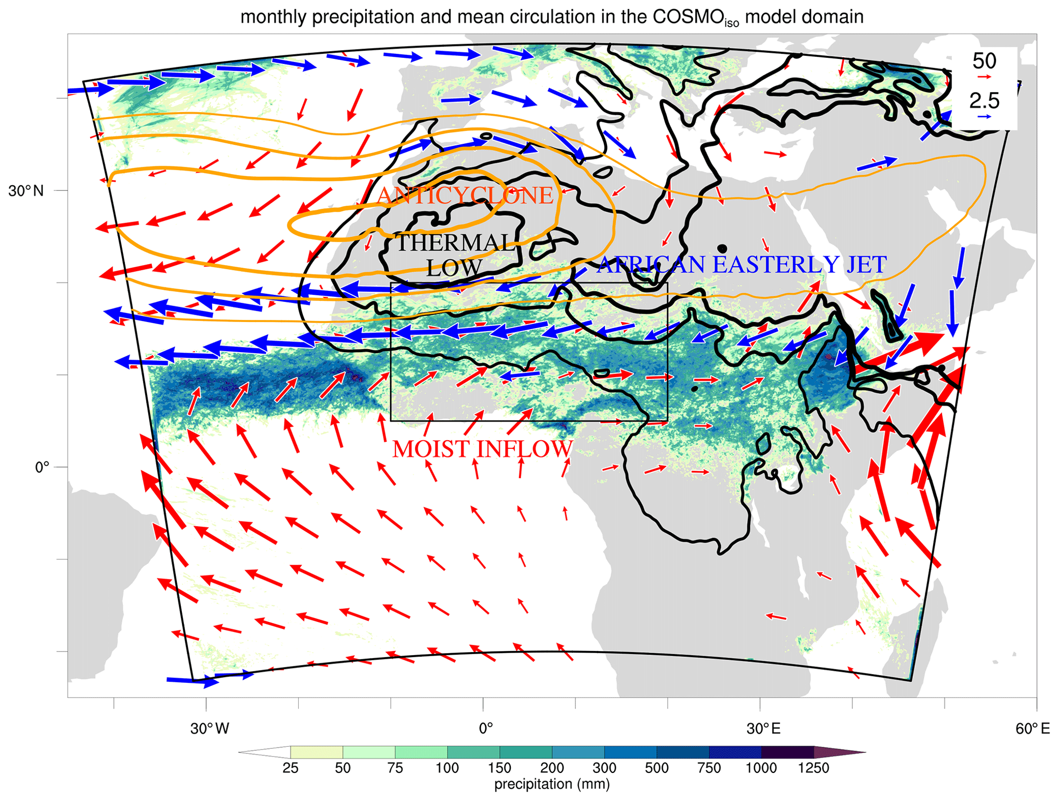
Figure 1Overview of the West African monsoon (WAM) system and the COSMOiso model domain. Monthly precipitation (mm; shading) and monthly mean circulation patterns (contours) from the convection-permitting COSMOiso simulation at a 7 km horizontal grid spacing for July 2016 are shown. The circulation patterns depict the Saharan heat low (mean sea level pressure, hPa; black contours), the mid-tropospheric anticyclone (500 hPa geopotential height, gpm; orange contours), the moist air inflow from the eastern tropical Atlantic (vertically integrated horizontal water vapour transport between 1000 and 850 hPa; red vectors where its magnitude >50 kg m−1 s−1), and the African easterly jet (600 hPa horizontal wind; blue vectors where the wind velocity >7 m s−1). The COSMOiso model domain (thick black contours) has a rotated grid centred at 13∘ N, 7.5∘ E. The box in the centre denotes the region of interest (thin black contours; 5–20∘ N, 10∘ W–20∘ E) used for the analysis in Sects. 3.1, 3.3, 4.2, 4.3, and 5.
One of the Earth's regions where convective systems are particularly strong and can affect the TTL is West Africa (Zipser et al., 2006; Cetrone and Houze, 2009; Fierli et al., 2011). In boreal summer, the atmospheric circulation over this region is dominated by the West African monsoon (WAM). The WAM system (Fig. 1) involves a complex interplay between different large-scale circulation and mesoscale convective processes (Redelsperger et al., 2002; Lacour et al., 2017; Diekmann et al., 2021b). Intense solar heating over the Sahara Desert leads to the formation of the Saharan heat low (Lavaysse et al., 2009), while much colder sea surface temperatures in the eastern tropical Atlantic cool the air near the surface. The resulting pressure gradient drives an inflow of moist air from the ocean into the continent's interior that feeds rainfall over this region. The tropical rain belt stretches zonally over Africa and is confined along its northern edge by the mid-tropospheric anticyclone aloft the Saharan heat low. The WAM follows a distinct seasonal evolution (Thorncroft et al., 2011): before its onset, the rain belt is anchored over the coast of Guinea, and it migrates abruptly northward into the Sahel after its onset, which usually takes place between late June and early July (Sultan and Janicot, 2003; Fitzpatrick et al., 2015). Precipitation over West Africa can stem from different types of convection embedded in the WAM circulation, whereby highly organized mesoscale convective systems (MCSs) contribute up to 90 % of rainfall (Mathon et al., 2002). MCSs typically traverse the Sahel in a westward direction, often along instabilities in the African easterly jet, known as African easterly waves (Fink and Reiner, 2003; Knippertz et al., 2017).
MCSs over West Africa are not only of central importance for precipitation but also for the formation of tropical ice clouds (Mathon and Laurent, 2001; Frey et al., 2011). Large MCSs are the most important contributor of tropical ice clouds over this region in summer (Yuan and Houze, 2010). Convective systems inject ice into the upper troposphere that is then detrained into large anvils that spread out into thinning cirrus shields (Luo and Rossow, 2004). Other types of ice clouds form directly from the vapour phase under the influence of gravity waves or uplift above convective systems (Pfister et al., 2001). These two formation pathways of ice clouds have been coined “liquid-origin” and “in situ” cirrus (Krämer et al., 2016, 2020; Luebke et al., 2016; Wernli et al., 2016; Gasparini et al., 2018). Liquid origin refers to the freezing of liquid water in updraughts within the mixed-phase cloud layer, whereas in situ refers to the formation of ice crystals directly from the vapour phase. Other classifications of cirrus ice clouds are based on environmental conditions such as synoptic weather systems, orographic lifting, and convective systems (Muhlbauer et al., 2014; Jackson et al., 2015; Gryspeerdt et al., 2018). Independent of these classifications, the life cycle of cirrus clouds consists of a formation and growth phase under the influence of freezing or nucleation and deposition, followed by the decay and disappearance of ice due to the fallout (sedimentation) and sublimation of ice particles. These processes have been clearly identified in the vertical structure of ice clouds based on observations and high-resolution model simulations (Urbanek et al., 2017; Gasparini et al., 2019) as well as in Lagrangian studies considering the cirrus life cycle along trajectories (Gasparini et al., 2021).
Stable water isotopes are a useful natural tracer of the Earth's water cycle (Galewsky et al., 2016), in particular for studying processes near tropical deep convection (Bony et al., 2008; Blossey et al., 2010). Besides the most abundant HO isotopologue, the Earth's water cycle also contains the much less abundant heavier HDO and HO isotopologues (Gat, 1996). Differences in their physical characteristics (saturation vapour pressure and molecular diffusivity) change their relative proportions during phase transitions, referred to as fractionation, whereby the heavier isotopes go preferentially into the solid or liquid phase compared with the vapour phase (Merlivat and Nief, 1967; Jouzel and Merlivat, 1984). As a result, isotopes contain information on an air parcel's history, making them a unique tool to study moist atmospheric processes, including precipitation, convection, and synoptic weather systems (Bony et al., 2008; Risi et al., 2008b, 2010b; Pfahl et al., 2012; Aemisegger et al., 2015; Weng et al., 2021). An important concept that helps with interpreting isotope information is Rayleigh distillation, which describes the progressive depletion of heavy isotopes in the vapour of cooling (e.g. moist adiabatically ascending) air, typically assuming that the forming condensate is instantly removed (Dansgaard, 1964). This principle explains, to a first order, the observed depletion of heavy isotopes in water vapour with latitude and altitude (Dansgaard, 1964; Rozanski et al., 1993). In the tropics, these effects are less prominent due to the relatively weak horizontal temperature gradients as well as strong convective transport and mixing that can dominate over horizontal transport. In these regions, there is often an anticorrelation observed between heavy isotopes in precipitation and precipitation amounts (Dansgaard, 1964; Rozanski et al., 1993). This effect can largely be explained by the strength of convection (Risi et al., 2020) and its degree of organization (Lawrence et al., 2004; Nlend et al., 2020). Stronger convection usually has larger rain droplets and occurs in a moister environment, reducing the re-evaporation of the falling condensate and leading to more depleted surface precipitation (Risi et al., 2008a; Torri et al., 2017). Similarly, strong, organized convection typically entrains more depleted vapour from higher altitudes and more efficiently depletes low tropospheric vapour than weak, isolated convection, eventually resulting in more depleted surface precipitation (Risi et al., 2008b; Moore et al., 2014).
Observations of water isotopes and modelling experiments equipped with isotope physics have improved our understanding of the atmospheric processes in monsoons and tropical convection in general. Global satellite-based measurements and general circulation model (GCM) simulations have shown that ocean evaporation and continental evapotranspiration provide enriched vapour that is transported into monsoon systems (Worden et al., 2007; Risi et al., 2010b; Brown et al., 2013). Air masses that move into the continent are gradually depleted due to rainout along their transport pathways, which is partly compensated for by continental moisture recycling (Risi et al., 2010b; Winnick et al., 2014). Large-scale subsidence can dehydrate and deplete vapour at the poleward edges of monsoon systems (Frankenberg et al., 2009; Risi et al., 2010b). Convective processes and their influence on water isotopes are more complex than the effects of large-scale circulation processes and limit our understanding and interpretation of isotope signals in atmospheric water. Satellite measurements suggest that shallow convection enriches mid-tropospheric vapour through the detrainment of enriched boundary layer air (Lacour et al., 2018), whereas deep convection enriches upper-tropospheric air due to convective detrainment at these altitudes (Randel et al., 2012). Experiments with a single-column model pointed to a variety of processes that can affect the isotopic composition of water vapour and precipitation in relation to tropical deep convection, including condensate lofting, rain re-evaporation, unsaturated downdraughts, and the isotopic exchange between droplets and the tropospheric environment (Bony et al., 2008; Risi et al., 2008a). Specifically, with regards to the WAM, in situ observations of precipitation isotopes have shown that its isotopic composition can reflect information about the type of convective organization (Risi et al., 2008b, 2010a).
Importantly, observations of stable water isotopes have offered novel insights into convective processes that affect the TTL and its water budget. The TTL demarcates the transition of the upper troposphere to the lower stratosphere in the tropics between altitudes of 14 and 18.5 km, corresponding to approximately 150 and 70 hPa (Fueglistaler et al., 2009). This region also contains the cold-point tropopause, with temperatures as low as 190 K near 90 hPa and 17 km altitude (Fueglistaler et al., 2009). Transport of air through this cold point leads to so-called “freeze-drying” of air as a result of the in situ formation of ice that subsequently falls out (Holton and Gettelman, 2001), thereby further depleting the remaining vapour from heavy isotopes. Previously, it was thought that the slow upwelling of air through this cold point, associated with the Brewer–Dobson circulation, controls the very low amounts of water vapour that can enter the lower stratosphere (Holton et al., 1995). Space-borne observations of stable water isotopes, however, showed that tropical lower-stratospheric water vapour is much more enriched than Rayleigh distillation predicts, suggesting other processes at work, such as tropical deep convection (Moyer et al., 1996; Kuang et al., 2003; Hanisco et al., 2007; Steinwagner et al., 2010). Indeed, subsequent in situ observations from aircraft measurements (Corti et al., 2008; Sayres et al., 2010) and modelling experiments (Ren et al., 2007; Wang et al., 2019; Bolot and Fueglistaler, 2021) showed that evaporation of convectively lofted ice moistens the lower TTL. Moreover, measurements over West Africa suggest that occasionally overshooting convection can directly moisten the lower stratosphere (Khaykin et al., 2009). A variety of model experiments equipped with stable water isotopes, such as conceptual models (Dessler and Sherwood, 2003), trajectory calculations (Dessler et al., 2007; Sayres et al., 2010), single-column models (Bony et al., 2008), large-eddy simulations (Smith et al., 2006), and GCM simulations (Eichinger et al., 2015), confirmed the influence of tropical convection on the TTL water budget. Idealized simulations with a two-dimensional cloud-resolving model suggested that the sublimation of convectively lofted enriched ice and fractionation of in situ cirrus cloud formation affect the water vapour in the TTL (Blossey et al., 2010). Accordingly, previous modelling studies that investigated the role of deep convection and ice cloud formation on the TTL water budget used idealized model set-ups, trajectory calculations with inherent limitations stemming from the underlying data, or relatively coarse-resolution model simulations with parameterized convection.
This study uses, for the first time, regional isotope-enabled convection-permitting model simulations constrained by actual meteorological conditions to investigate the atmospheric processes related to tropical deep convection and cirrus clouds in the WAM. The purpose of this work is twofold: (1) to identify the processes related to tropical ice cloud formation and decay based on stable water isotope information and (2) to examine the influence of deep convection on TTL water vapour and its isotopic composition. We use simulations with the Consortium for Small-Scale Modelling isotope-enabled (COSMOiso) model (Pfahl et al., 2012) at different resolutions and with different treatments of convection over West Africa for the period from June to July 2016 (Sect. 2). First, we evaluate the model simulations by comparing the isotopic composition of water vapour and monthly precipitation to observations. In addition, we assess the model's ability to simulate the monsoon evolution and behaviour of convective storms through comparison of precipitation characteristics in model output against satellite-based precipitation observations (Sect. 3). Next, we switch focus to tropical ice clouds and explore the isotopic imprints of deep convection on atmospheric water in a case study, followed by a detailed statistical analysis (Sect. 4). In Sect. 5, we use total column ice amounts as a simple proxy to distinguish between different types of ice cloud regimes, and we examine their different isotope signals. Finally, Sect. 6 concludes this study with a summary of the results, including a synthesis of five different key processes related to the formation and decay of tropical ice clouds derived from isotope information.
2.1 The COSMOiso model
The Consortium for Small-Scale Modelling (COSMO) model (Steppeler et al., 2003) is a non-hydrostatic limited-area weather and climate model used for operational forecasting and research purposes. Stable water isotopes HDO and HO are implemented in the model (COSMOiso) by adding parallel water cycles for both heavy isotopes that are purely diagnostic and do not affect any other model components (Pfahl et al., 2012). These heavy isotopes and the common water isotope HO undergo identical processes except during phase transitions when isotopic fractionation occurs. COSMOiso has been used to study a variety of atmospheric processes in the hydrological cycle in idealized studies (Dütsch et al., 2016), detailed case studies (Pfahl et al., 2012; Aemisegger et al., 2015; Lee et al., 2019), and (semi-)climatological analyses (Dütsch et al., 2018; Christner et al., 2018; Dahinden et al., 2021; Diekmann et al., 2021b; Thurnherr et al., 2021).
This study uses the isotope-enabled COSMO model version 4.18 with a prognostic one-moment bulk microphysics scheme (Doms et al., 2005). Water is represented by five species: vapour, cloud ice, snow, cloud water, and rain. Cloud water and cloud ice represent small droplets and pristine ice crystals with negligible fall velocities. Rain and snow represent larger droplets and ice particles respectively, with fall velocities that are computed from size distribution functions and empirically derived relations based on measurements (Doms et al., 2005).
Fractionation occurs during the phase changes from vapour to liquid (condensation), vapour to ice (nucleation and deposition), and liquid to vapour (evaporation). Fractionation at thermodynamic equilibrium is parameterized using equilibrium fractionation factors with respect to liquid water and ice, following Majoube (1971) and Merlivat and Nief (1967) respectively. Non-equilibrium effects are taken into account by a combined fractionation factor (Jouzel and Merlivat, 1984; Blossey et al., 2010). These effects occur, for instance, if the air is supersaturated with respect to ice, such as during the Wegener–Bergeron–Findeisen effect in mixed-phase clouds. Non-equilibrium effects arising from ice surface kinetics (Nelson, 2011) are neglected in the model. During freezing, melting, and sublimation, no fractionation occurs. For more information on the representation of fractionation during phase changes in the cloud microphysics scheme of COSMOiso, see Pfahl et al. (2012).
Surface evaporation from oceans is parameterized using the Craig–Gordon model (Craig and Gordon, 1965), representing non-equilibrium fractionation based on an empirically derived relation independent of wind speed (Pfahl and Wernli, 2009). For the isotopic composition of seawater, we use ECHAM5-wiso data from Werner et al. (2011), which is based on an observational dataset for δ18O (LeGrande and Schmidt, 2006). The δ2H of sea surface water is assumed to follow the relation of global meteoric waters (Craig and Gordon, 1965) and is, thus, equal to the δ18O multiplied by a factor of 8. Land–atmosphere interactions are represented by a multilayer land surface scheme equipped with water isotopes, accounting for processes such as plant transpiration and bare-soil evaporation; the reader is referred to the supplement of Christner et al. (2018) for more details.
Table 1Overview of the three model simulations and their configurations.
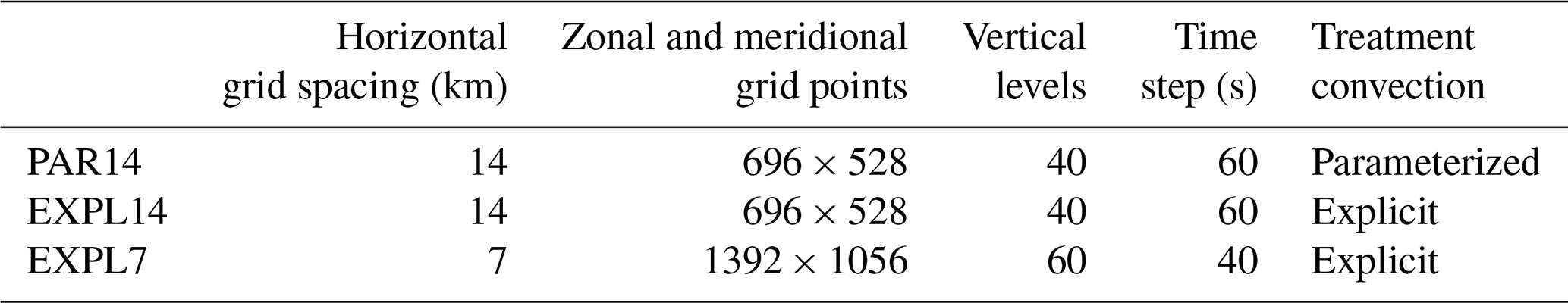
2.2 Model simulations
The COSMOiso model simulations are performed on a rotated grid centred at 13.0∘ N, 7.5∘ E. The model domain covers the larger part of the African continent, the eastern and tropical Atlantic, the Mediterranean, and the western margins of the Indian Ocean (Fig. 1). This relatively large model domain allows for the explicit simulation of different inflow airstreams into the WAM system and the processes that affect the isotopic composition of water along these transport pathways (Diekmann et al., 2021b). We perform three model simulations with different configurations in terms of their resolution and treatment of convection (Table 1). The first simulation, PAR14, has a horizontal grid spacing of 14 km, 40 model levels, and convection is parameterized using the scheme by Tiedtke (1989). The second simulation, EXPL14, has an identical resolution, but the convection parameterization scheme is switched off. The third simulation, EXPL7, also has a convection-permitting set-up (i.e. no parameterized convection) but at a higher resolution, with a 7 km horizontal grid spacing and 60 model levels reaching up to 23.6 km a.s.l. For both convection-permitting simulations, the shallow-convection scheme is also switched off, as stable water isotope tracers are not implemented in the shallow-convection scheme in COSMOiso.
The motivation for these different model experiments is that it is not a priori clear how the isotope-enabled model performs in the convection-permitting set-up for the WAM. Most previous studies used COSMOiso in mid-latitude or polar regions with parameterized convection. For our present study, it is highly advantageous to switch off the convection scheme, allowing the explicit simulation of deep moist convection in the tropics. This model set-up will benefit the interpretation of isotope signals in ice clouds, circumventing the drawbacks of the simplified cloud microphysics in the convection parameterization scheme and the complex interactions of convection and cloud microphysics schemes in cirrus layers. Moreover, previous studies have found that the hydrological cycle and deep moist convection in the WAM is much better represented in convection-permitting simulations than with parameterized convection (Marsham et al., 2013; Birch et al., 2014). Our choice for relatively coarse-resolution simulations, considering the usual standards for a convection-permitting set-up, is further motivated by new insights into the fact that parameterization schemes can be switched off at coarser resolutions than previously thought – that is, on the order of ∼10 km (Vergara-Temprado et al., 2020). This resolution also allows for the use of a large model domain in which the regional model can generate its own hydrological cycle and isotope meteorology without being too strongly affected by the boundary information from the driving global model output.
Our COSMOiso simulations are initialized and driven by 6-hourly updated fields at the lateral boundaries from global ECHAM5-wiso output (Werner et al., 2011). This output is produced by global isotope-enabled ECHAM5 simulations with a T106 spectral resolution and 31 model levels, nudged to the dry atmospheric state of the ERA-Interim reanalysis (Butzin et al., 2014). Within the model domain, the COSMOiso simulations are relaxed towards the driving global output by spectral nudging (von Storch et al., 2000) of the large-scale horizontal winds above 850 hPa (wave numbers 5 and less). In this way, the large-scale circulation within the regional domain is kept close to real conditions while smaller-scale processes, including deep moist convection, are fully treated by COSMOiso. The COSMOiso model simulations are integrated for the 2-month period of the “Dynamics–Aerosol–Chemistry–Cloud Interactions in West Africa” (DACCIWA) field campaign from 1 June to 30 July 2016. Hourly output is produced on model levels and interpolated to 29 pressure levels with 50 hPa intervals between 750 and 250 hPa and 25 hPa intervals in the 1000–750 and 250–50 hPa pressure layers.
2.3 Observations
For the purpose of model evaluation, we compare our model simulation output to stable water isotope observations of tropospheric water vapour and surface precipitation as well as satellite-based precipitation estimates. More specifically, we use space-borne measurements of the Infrared Atmospheric Sounding Interferometer (IASI) sensor on board EUMETSAT (European Organization for the Exploitation of Meteorological Satellites) satellites. This dataset is an extension of the MUlti-platform remote Sensing of Isotopologues for investigating the Cycle of Atmospheric water (MUSICA; Schneider et al., 2016, 2022). We use the Level-3 data, which are quality controlled and available on a regular 1∘ × 1∘ grid at a mid-tropospheric altitude of approximately 4220 m a.s.l. (Diekmann et al., 2021a). This dataset contains twice-daily estimates of the humidity and δ2H under cloud-free conditions.
Furthermore, we also use monthly observations from the Global Network for Isotopes in Precipitation (GNIP). GNIP data are collected by the International Atomic Energy Agency (IAEA) and World Meteorological Organization (WMO) (Rozanski et al., 1993; Araguas-Araguas et al., 2000). We use monthly observations from 19 stations over equatorial and North Africa. Several stations record only δ values of 18O and 2H in precipitation and miss the actual precipitation amounts. For this reason, we refrain from computing mass-weighted means over the 2-month simulation period, and we compare the model output to the observations for the 2 individual months (see Sect. 3.2). Note that the evaluation of our model output against GNIP observations is limited due to the relatively low station density over North Africa and available precipitation measurements at monthly timescales. Nevertheless, we consider the inclusion of GNIP data in our model evaluation as an asset, as these data contain information about cloud and below-cloud processes in the water cycle which are only indirectly included in the IASI data, which only cover cloud-free regions.
Finally, we use monthly and hourly satellite-based precipitation estimates from the Integrated Multi-satellitE Retrievals for the Global Precipitation Measurement (GPM) Mission (IMERG) dataset (Huffman et al., 2020) to evaluate the spatial distribution of precipitation, the evolution of the monsoon, and the motion of convective storms in our model simulations.
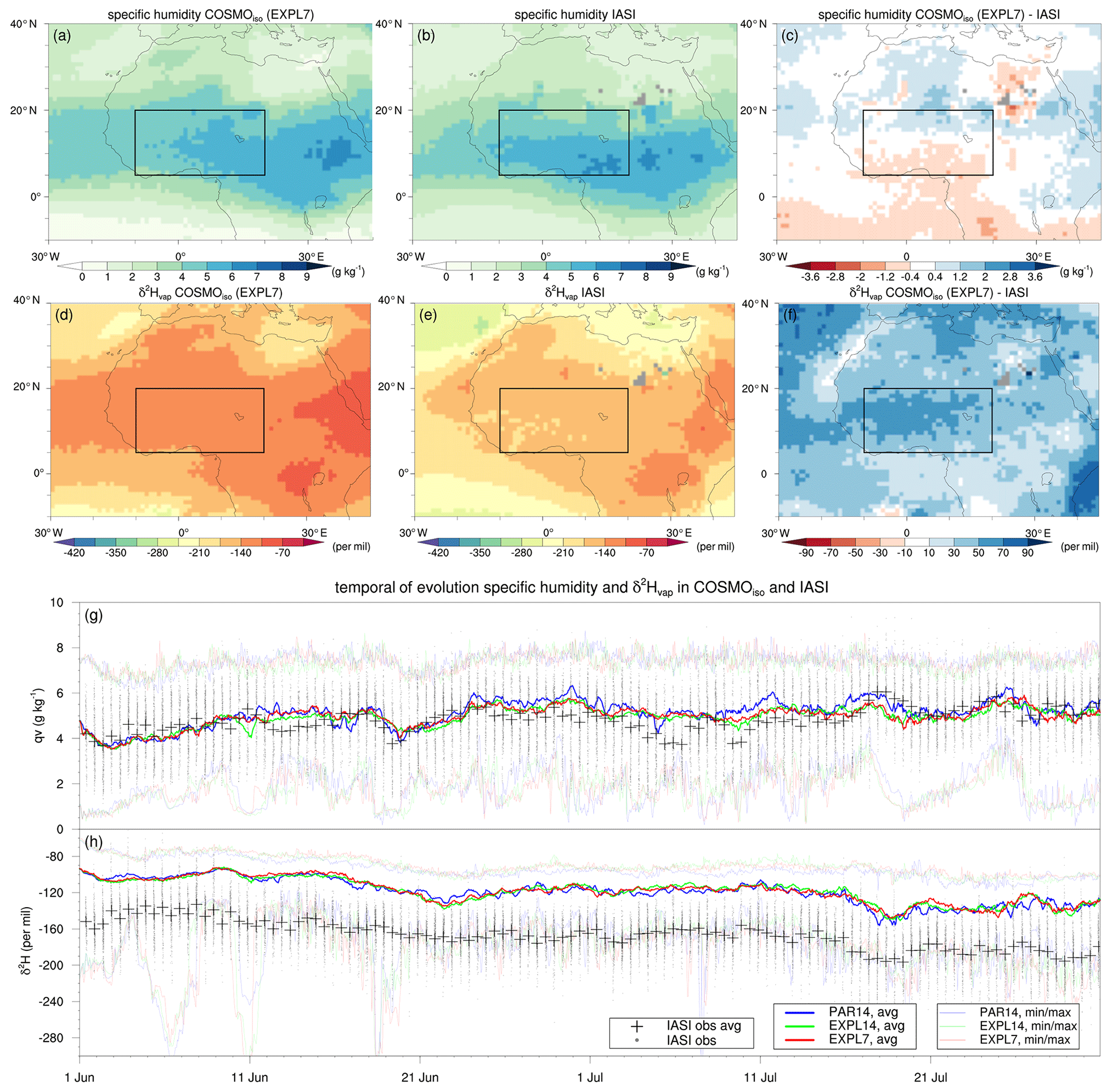
Figure 2Spatial distribution and temporal evolution of specific humidity and water vapour isotopes in COSMOiso and IASI observations at 4220 m a.s.l. for the 2-month simulation period of June–July 2016. The panels show the (a–c) specific humidity (g kg−1) and (d–f) δ2H in water vapour (‰) from (a, d) EXPL7, (b, e) IASI, and (c, f) the difference between EXPL7 and IASI. The bottom panels show the temporal evolution of (g) specific humidity (g kg−1) and (h) δ2H in vapour (‰) based on domain averages and minima and maxima values for grid points in the region of interest (see Fig. 1) for all three COSMOiso model simulations and IASI observations, as indicated by the legend. For COSMOiso output, only data where the sum of total column cloud ice, snow, liquid water, and rain (TQ) remains below a threshold of 0.01 kg m−2 are used; see the text for details.
3.1 IASI water vapour isotope observations
Figure 2 compares specific humidity and the water vapour isotopic composition (δ2Hvap) from COSMOiso model simulations against IASI observations. We use COSMOiso model output at 09:00 and 21:00 UTC, because IASI observations in the morning and evening fall within the time windows of 07:00–10:00 UTC and 19:00–22:00 UTC respectively. To facilitate the comparison, we interpolate the model output from its rotated grid at model levels to a regular 1∘ × 1∘ horizontal grid at 4220 m a.s.l. In this comparison, we only include the model output where the sum of total column cloud ice, snow, cloud water, and rain (TQ) remains below a threshold of 0.01 kg m−2 as a proxy for cloud-free regions. Applying this threshold results in 51.3 % of “cloud-free” grid points in the model output in the region of interest (5–20∘ N, 10∘ W–20∘ E) during the 2-month simulation period compared with 55.8 % of grid points with non-missing values in the IASI data. Figure 2a–f show the spatial distribution of specific humidity and δ2Hvap from EXPL7 and IASI averaged over the 2-month simulation period. Figure 2g and h show the temporal evolution of the two variables at individual grid points and their domain averages over the region of interest for all three model simulations and observations.
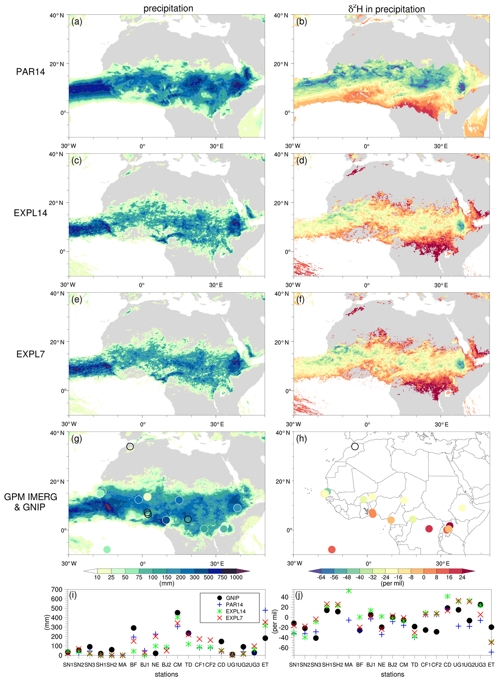
Figure 3Monthly precipitation and its isotopic composition from the three model simulations and GNIP observations for July 2016. The panels show (left) precipitation amounts (mm) and (right) δ2H in precipitation (‰) in (a, b) PAR14, (c, d) EXPL14, (e, f) EXPL7, (g, h) GNIP observations, and (i, j) GNIP observations and COSMOiso simulation output, as indicated by the legend, at station locations. Precipitation outside the circles in panel (g) is from GPM IMERG, and open black circles in panels (g) and (h) denote missing values. COSMOiso output in panels (i) and (j) is interpolated at the station locations, and values are only plotted if the simulated precipitation amounts are larger than 1 mm per month. GNIP stations in panels (i) and (j) are ordered by longitude from west to east: (SN1) Dakar Yoff, (SN2) Pout, (SN3) Louga, (SH1) Ascension Island, (SH2) Travellers Hill, (MA) Fes Sais, (BF) Bobo-Dioulasso, (BJ1) Bohicon, (NE) Niamey, (BJ2) Cotonou, (CM) Douala-Hydrac, (TD) N'Djamena, (CF1) Bangui-Universite, (CF2) Bangui-Sodeca, (CD) Kisangani, (UG1) Entebbe, (UG2) Jinja, (UG3) Bugondo, and (ET) Addis Ababa.
The specific humidity in EXPL7 and IASI shows good spatial agreement overall (Fig. 2a, b, c). Apart from a weak dipole structure with moister air over the Sahara and drier air over the Gulf of Guinea and the tropical Atlantic in the model compared with IASI, their differences are relatively small and on the order of 1–2 g kg−1. This good agreement between the model and observations is noted across all three model simulations, both in terms of their spatial distribution (not shown) and temporal evolution (Fig. 2g). However, a clear systematic deviation emerges in δ2Hvap, which is consistently more enriched in the model compared with IASI, by approximately 50 ‰ (Fig. 2d, e, f, h). This deviation between the model and observations is consistently present for all three model simulations. Among the simulations, only very small to negligible differences arise in terms of their spatial distribution (not shown) and temporal evolution (Fig. 2h). Currently, this difference in δ2Hvap between COSMOiso and IASI is not understood and may stem from uncertainties in both the model and observations. Previous studies have also noted a positive difference in vapour isotopes in models compared with observations (Werner et al., 2011; Risi et al., 2012; Christner et al., 2018). Despite this systematic deviation, the δ values in the model simulations and observations follow a very similar temporal evolution throughout the 2-month simulation period (Fig. 2h). Accordingly, the Pearson correlation based on the twice-daily domain average δ2Hvap values in the simulations and IASI reaches high values of 0.90, 0.87, and 0.88 for PAR14, EXPL14, and EXPL7 respectively. The relatively similar performance between the different model simulations may stem from the use of domain averages as well as the exclusion of cloudy regions where the largest difference between model simulations may be expected. Therefore, we proceed with a comparison of isotopes in surface precipitation which includes the effects of fractionation in the water cycle during condensation, deposition, and below-cloud sublimation and evaporation.
3.2 Precipitation isotopes from GNIP stations
Figure 3 shows monthly precipitation and its isotopic composition for the three model simulations and the GNIP observations in July 2016 (for June 2016, see Fig. S1 in the Supplement). We first discuss the spatial patterns in precipitation isotope signals in the three model simulations and then compare them to GNIP observations.
At first glance, precipitation generally displays a similar pattern in the three model simulations. Precipitation occurs in a zonal band between 0 and 20∘ N that reflects the tropical rain belt as a part of the Intertropical Convergence Zone (Fig. 3a, c, e), which is in agreement with the GPM IMERG precipitation observations (Fig. 3g). δ2H in precipitation is generally more depleted in the centre of the rain belt where rainfall amounts are highest (Fig. 3b, d, f), consistent with previous studies on isotopes in tropical precipitation (e.g. Dansgaard, 1964; Rozanski et al., 1993; Risi et al., 2008a). Upon closer scrutiny, we note substantial spatial gradients in precipitation isotope signals. They are particularly visible in the convection-permitting simulations (Fig. 3d, f) and reflect three different processes: (1) enriched precipitation over the coast of Guinea that depletes towards the Sahel region due to the gradual depletion of land-inward moving moist air from the tropical Atlantic, although this is partly compensated for by continental recycling (Risi et al., 2010b; Winnick et al., 2014); (2) very enriched precipitation over Central Africa, likely due to the influence of non-fractionating transpiration in this densely vegetated region (Aemisegger et al., 2014; Galewsky et al., 2016); and (3) very enriched precipitation along the northern fringe of the rain belt as a result of strong below-cloud effects, i.e. enhanced evaporation of falling rain in the warm and dry environment (Risi et al., 2008b).
Comparing the precipitation and its isotopic composition among the three different model simulations, we observe larger differences between the convection-parameterized and convection-permitting simulations than between the convection-permitting simulations at different resolutions. Generally, precipitation in the parameterized convection simulation has larger amounts and is more depleted compared with both convection-permitting simulations (Fig. 3a, b, c, d, e, f). Most likely, these differences stem from the way precipitation processes (convective and large-scale components) are represented in the different model configurations. Switching off the parameterization scheme strongly changes the hydrological cycle, consistent with previous studies that focused on the WAM region (Marsham et al., 2013; Birch et al., 2014; Pante and Knippertz, 2019).
Table 2RMSE of precipitation in the three COSMOiso experiments compared with GNIP observationsa,b.
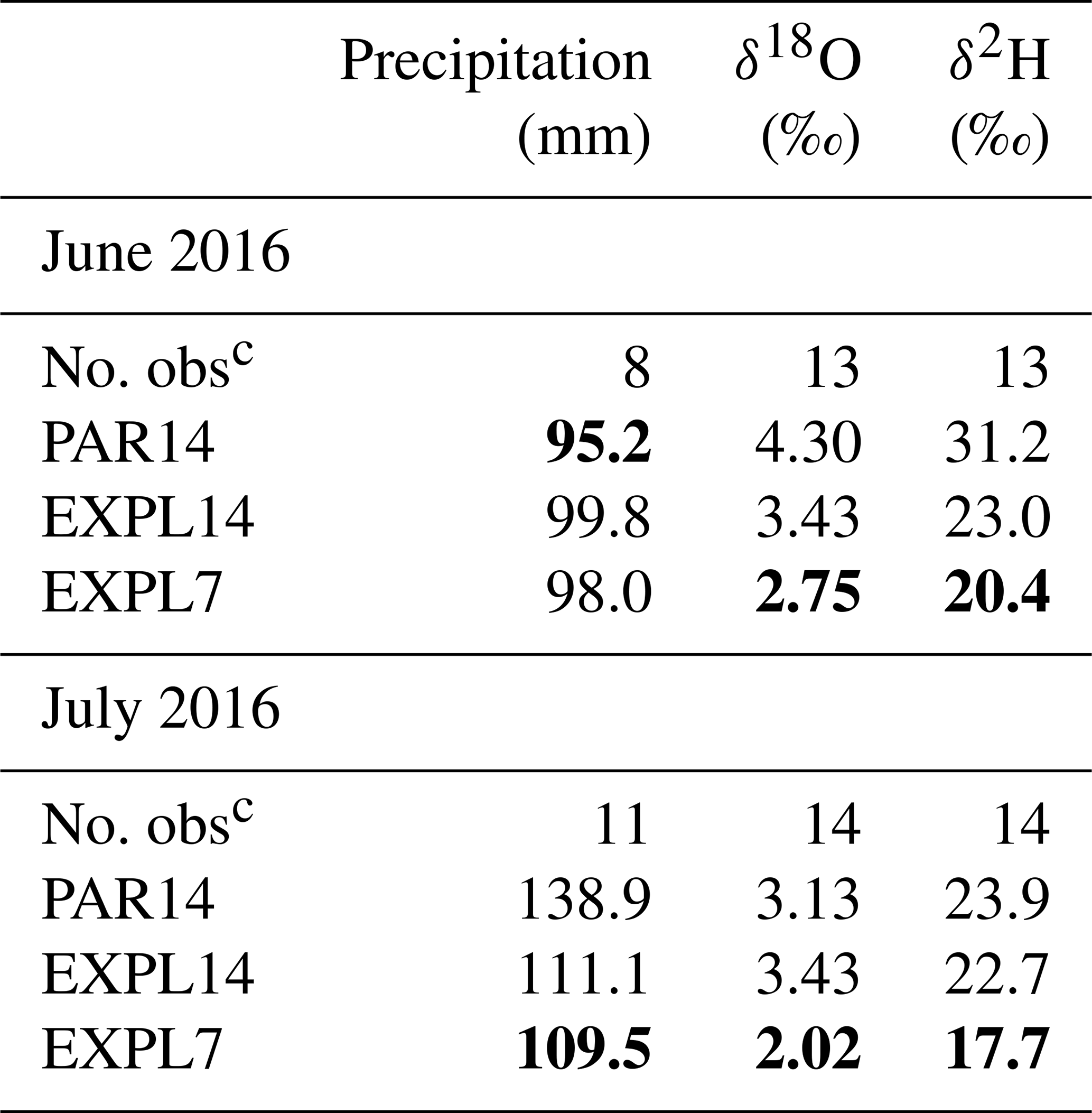
a RMSE values are based on station locations where all three simulations have precipitation amounts >20 mm per month. b The best skill scores across the three model simulations are shown in bold. c The number of station locations with valid data – that is, non-missing values in GNIP and precipitation amounts >20 mm per month in all three model simulations.
Table 3ME of precipitation in the three COSMOiso experiments compared with GNIP observationsa,b.
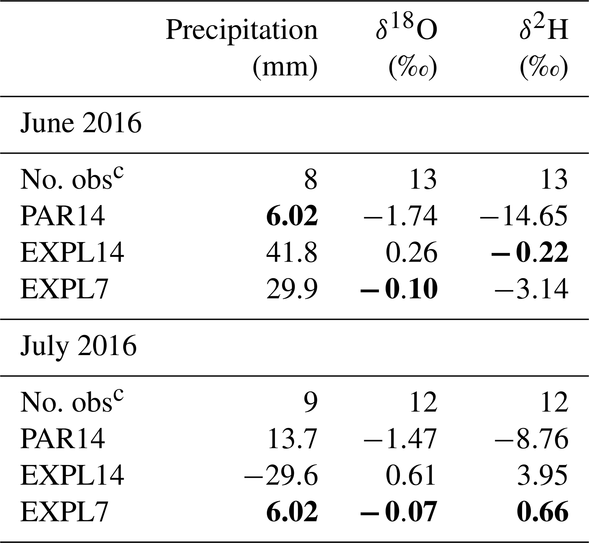
a ME values are based on station locations where all three simulations have precipitation amounts >20 mm per month. b The best skill scores across the three model simulations are shown in bold. c The number of station locations with valid data – that is, non-missing values in GNIP and precipitation amounts >20 mm per month in all three model simulations.
GNIP precipitation and its isotopic composition follow a similar spatial distribution to that of the COSMOiso simulations (Fig. 3g, h). Precipitation is relatively enriched along the coast of Guinea and Central Africa and more depleted in the Sahel (Fig. 3h). For a quantitative comparison of the simulations to observations, we interpolate the COSMOiso output to the station locations (Fig. 3i, j). Overall, we observe that the COSMOiso simulations follow the GNIP values reasonably well. A few interesting deviations appear that can be clarified by physical arguments. For example, for a station in Uganda (UG2), the convection-permitting simulations underestimate the precipitation amounts, going along with overly high δ2H in precipitation compared with GNIP (Fig. 3i, j). This suggests too much below-cloud rain evaporation, overly shallow clouds, or overly low precipitation efficiency in these simulations at this location, consistent with overly enriched surface precipitation. In contrast, for the station in Ethiopia (ET) all three model simulations overestimate rainfall amounts and simulate overly low δ2H compared with observations, showing that biases in simulated precipitation amounts are consistent with biases in δ2H in precipitation. Likewise, in June 2016 (Fig. S1i, j), the simulations overestimate precipitation amounts and have overly depleted precipitation compared with the GNIP observations at both stations in Uganda (UG2) and Ethiopia (ET).
Based on the GNIP observations and model output interpolated at station locations, we compute the root mean square error (RMSE) and mean error (ME) of the model simulations compared with the observations (Tables 2 and 3 respectively). The RMSE of the isotope variables (δ18O and δ2H) is lowest for the EXPL7 simulation in both months, indicating that the convection-permitting simulation at 7 km performs better than both simulations at 14 km. At 14 km resolution, there is no clear difference between the parameterized and explicit convection set-up, as EXLP14 performs better than PAR14 in June, whereas no clear differences emerge between both simulations for July (Table 2). Mean errors show that the convection-parameterized simulation consistently produces overly depleted precipitation, as also found in a 30-year climatological study for central Europe (Dütsch et al., 2018). In contrast, the convection-permitting simulation at 14 km mostly produces overly enriched surface precipitation.
This brief model evaluation demonstrates that the COSMOiso simulations are in good overall agreement with the GNIP observations. Moreover, previous studies have demonstrated a generally good agreement between COSMOiso simulations and observations of isotopes in vapour and precipitation (Pfahl et al., 2012; Aemisegger et al., 2015; Dütsch et al., 2018; Christner et al., 2018; Dahinden et al., 2021). The convection-permitting simulation at 7 km (EXPL7) outperforms both simulations at 14 km and, therefore, will be used for the remaining part of this study to analyse tropical ice clouds in the WAM of summer 2016. Before switching focus to tropical ice clouds, we briefly discuss the motion of convective storms in the EXPL7 simulation based on the evolution of precipitation during the monsoon period compared to GPM IMERG observations.
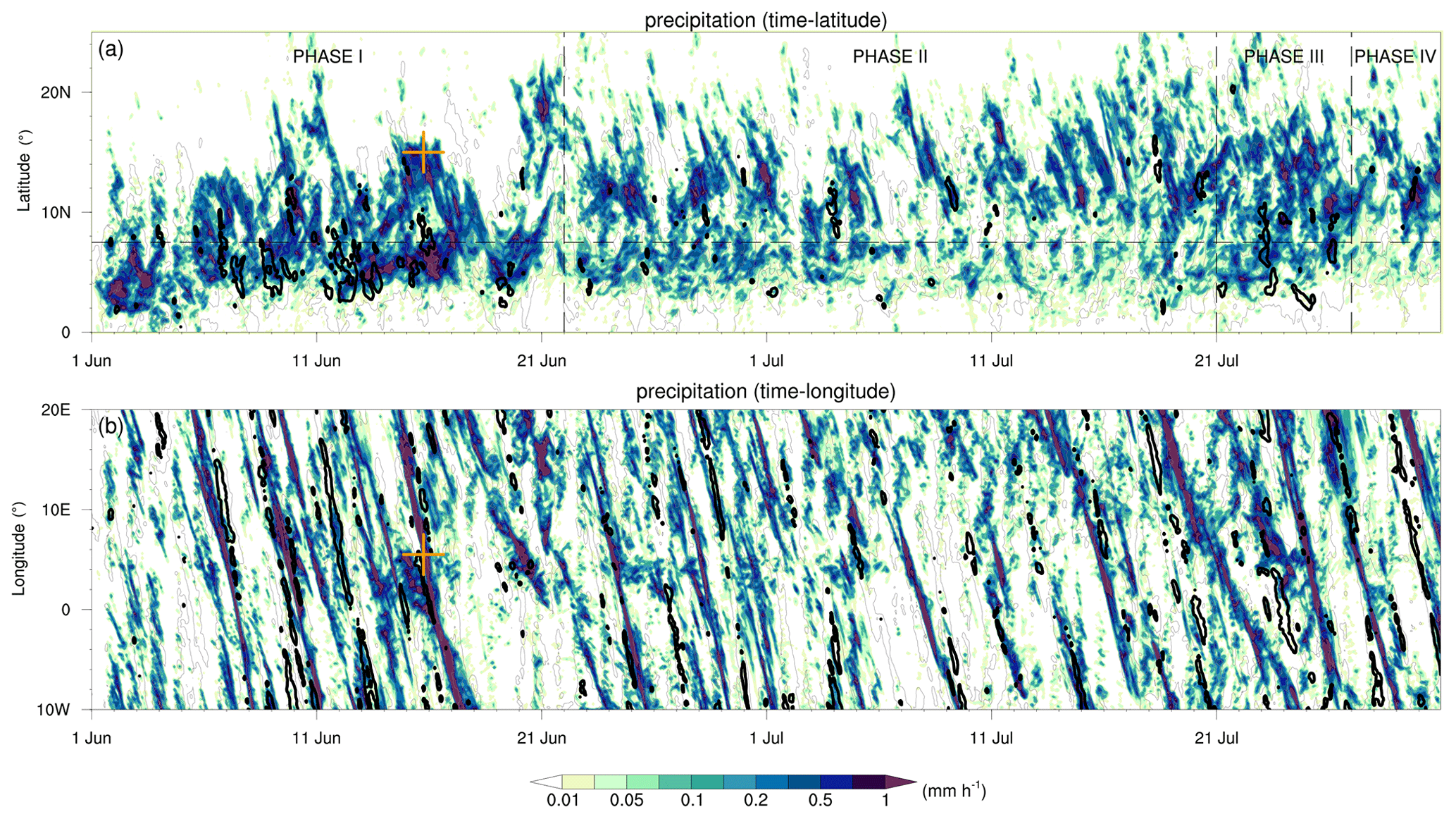
Figure 4The temporal evolution of precipitation from EXPL7 and GPM IMERG during the June–July 2016 period. The panels show precipitation (mm h−1) from EXPL7 (colours) and from GPM IMERG at 0.1 mm h−1 (thin grey contours) and 1.0 mm h−1 (thick black contours) (a) as a function of time and latitude averaged over the longitude band of 10∘ W to 20∘ E and (b) in a Hovmöller diagram averaged over the latitude band from 5 to 20∘ N. The four phases in panel (a) refer to the WAM stages discussed in Sect. 3.3, and the orange markers in panels (a) and (b) denote the time and location of the MCS discussed in the case study in Sect. 4.1.
3.3 Monsoon evolution and convective storm characteristics
The period from June to July 2016, when the DACCIWA field campaign took place, was characterized by four phases in the WAM evolution: (1) the pre-onset until 21 June, (2) the post-onset from 22 June to 20 July, (3) a wet phase from 21 to 26 July, and (4) a return to undisturbed monsoon conditions from 27 to 31 July (Knippertz et al., 2017). These four phases are reasonably well represented in the EXPL7 simulation, as shown by the latitudinal distribution of precipitation (Fig. 4a). Before the monsoon onset (phase 1), precipitation is predominantly confined to lower latitudes across the coast of Guinea (∼0–7.5∘ N). After the monsoon onset (phase 2), the rain belt has migrated northward and is positioned over the Sahel region (7.5–15∘ N). During the wet episode from 21 to 26 July (phase 3), large precipitation amounts occur over both the coast of Guinea and the Sahel. Afterwards, more usual monsoon conditions follow until the end of July (phase 4), with precipitation primarily centred over the Sahel. This evolution follows the GPM IMERG precipitation observations (grey and black contours in Fig. 4a), except for a rain belt that is positioned slightly too far northward in EXPL7. Our model simulates the monsoon onset 1–2 d too early (19–20 June) but captures the abrupt northward shift of precipitation into the Sahel well (Fig. 4a).
Figure 4b shows a Hovmöller diagram with average precipitation over the latitude band from 5 to 20∘ N as a function of time and longitude. Precipitation patterns clearly demonstrates long-lived MCSs that move from east to west over the course of several days. Comparison against GPM IMERG precipitation estimates (again in grey and black contours in Fig. 4b) show a generally realistic behaviour of the storms in our model when bearing in mind that convective systems cannot be expected to be simulated at the right time and place. Overall, EXPL7 represents a realistic evolution of the monsoon and MCS behaviour, providing further confidence in our model simulations. On 15 June 2016, an intense MCS passed our region of interest, as reflected by large precipitation amounts on this day (see the orange markers in Fig. 4a and b). This specific MCS is chosen for a case study to explore the isotope signatures of tropical deep convection in atmospheric water.
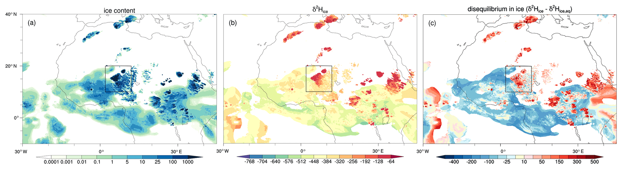
Figure 5Spatial distribution of ice and its isotopic composition at 200 hPa at 18:00 UTC on 15 June 2016 for the (a) ice content (mg kg−1), (b) δ2H in ice (‰), and (c) disequilibrium in ice (‰); see the text for details. Variables in all panels are transparent when the ice content values are below 10−4 mg kg−1.
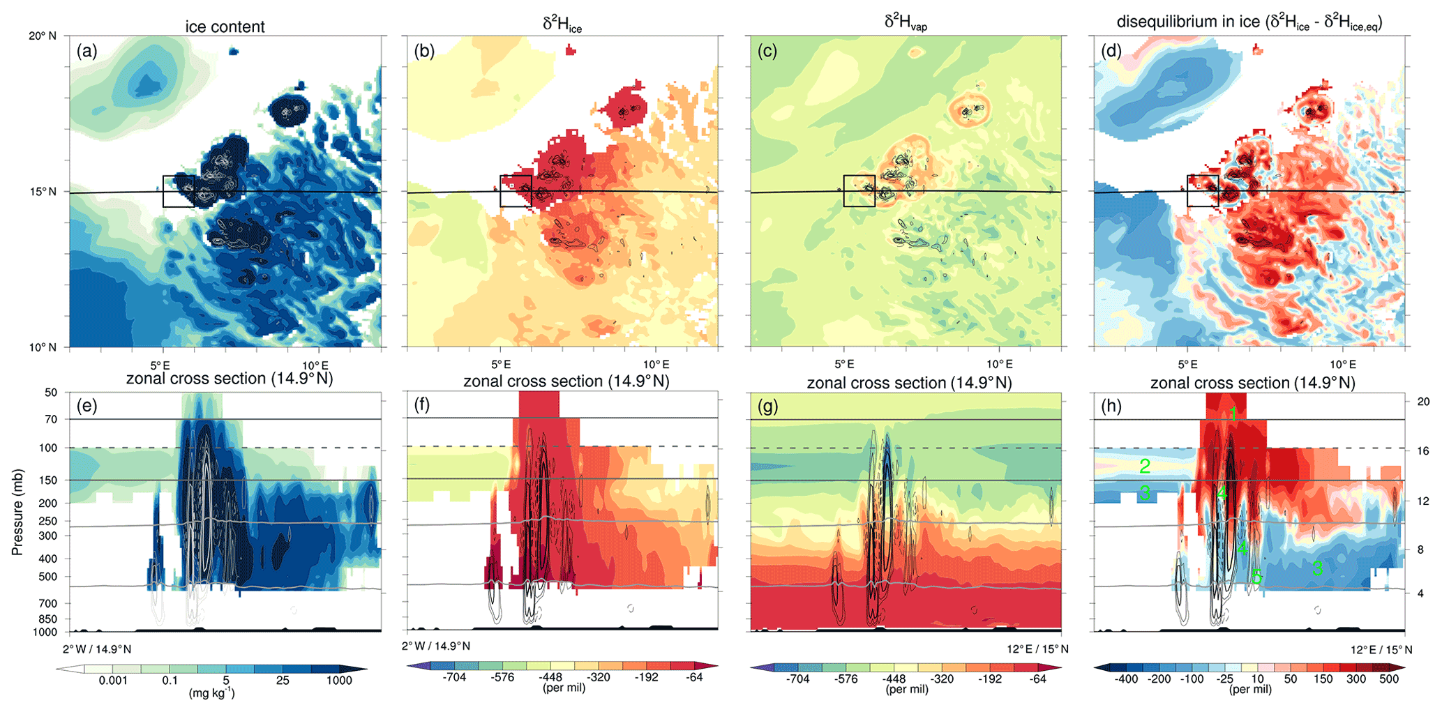
Figure 6As in Fig. 5 but for a smaller region (10–20∘ N, 2–12∘ E; as indicated by the black boxes in Fig. 5a–c) and at 16:00 UTC on 15 June 2016. In addition, panel (c) shows δ2H in vapour (‰), and panels (e)–(h) show vertical cross sections in a zonal direction along the black line in panels (a)–(d). The light grey contours in the cross sections are the isotherms at T=0 ∘C and ∘C to denote the liquid, mixed-phase, and ice cloud layers; the dark grey solid contours indicate the TTL region between 150 and 70 hPa; and the dark grey dashed contour indicates the approximate tropopause cold point near 100 hPa. The very light grey contours in panels (a) and (e) and the black contours in panels (b)–(d) and panels (f)–(h) show upward (downward) vertical motion using solid (dashed) lines at intervals of 1, 2, 5, and 10 m s−1 in panels (a)–(d) and at intervals of 0.5, 1, 2, 5, and 10 m s−1 in panels (e)–(h). The labels 1–5 in panel (h) refer to the processes discussed in Sect. 4.1.
4.1 An MCS case study
Figure 5 shows the spatial distribution of ice and its isotopic composition at 200 hPa at 18:00 UTC on 15 June 2016. Here and throughout this paper, ice content is defined by the sum of cloud ice and snow, unless explicitly mentioned otherwise (Fig. 5a). Similarly, δ2H in ice refers to the δ values in the mass-weighted sum of cloud ice and snow (Fig. 5b). Figure 5c shows the deviation of the isotopic composition of ice (δ2Hice as in Fig. 5b) from the ice that would form from local vapour under equilibrium fractionation. This variable, hereafter referred to as disequilibrium in ice, is defined by
Here, equilibrium ice δ2Hice,eq is temperature dependent and is computed using the same fractionation factor as in COSMOiso, , where T is the temperature (Merlivat and Nief, 1967; Rowley and Garzione, 2007). This approach follows the rationale of Aemisegger et al. (2015) and Graf et al. (2019), who used the disequilibrium of precipitation isotopes from vapour isotopes to investigate the influence of below-cloud effects during the passage of cold fronts in Europe. Disequilibrium in ice can result from non-equilibrium conditions during ice formation, and, of primary interest in this study, the absence of equilibrium exchanges between vapour and ice allows for a preservation of the isotope signal of convectively lofted ice in the upper troposphere and the TTL. Appendix A presents detailed information on the definition and interpretation of the concept of disequilibrium in ice that is introduced in this study.
Across equatorial Africa, we note multiple convective systems that reach the upper troposphere, characterized by large ice content >1000 mg kg−1 (Fig. 5a). The ice is very enriched with δ2H values near −100 ‰ (Fig. 5b), indicating that the convective systems bring large amounts of very enriched ice, which has formed at low altitudes from vapour deposition or through freezing liquid, into the upper troposphere. This is confirmed by large positive Δδ2Hice values that exceed +300 ‰ within these convective systems (Fig. 5c). Farther away from the convective systems we observe much lower amounts of ice (<25 mg kg−1), typical of cirrus clouds, which is much more depleted ( ‰ to −350 ‰) and has near-zero to negative Δδ2Hice values. Neutral Δδ2Hice is consistent with the in situ formation of ice from local vapour under equilibrium fractionation, whereas negative Δδ2Hice likely reflects the sedimentation of ice from aloft, being relatively depleted with respect to the ambient vapour at these altitudes.
Figure 6 zooms in on an MCS in the centre of the model domain (see boxes in Fig. 5a–c) at 16:00 UTC on 15 June 2016. In addition to the information given in Fig. 5, Fig. 6 also shows the δ2H in vapour (Fig. 6c), vertical cross sections in the zonal direction (Fig. 6e, f, g, h), and vertical motion contours. In the zonal cross sections, the liquid, mixed-phase, and ice cloud layers are denoted by the light grey contours (at T=0 and −38 ∘C), the TTL region is indicated by the dark grey contours (at 150 and 70 hPa), and the approximate cold-point tropopause is demarcated by the dashed dark grey contour at 100 hPa (Fig. 6e, f, g, h). Based on this figure and its time sequence (not shown), we observe how convective updraughts within the MCS inject enriched ice into the upper troposphere. This enriched ice remains in the middle and upper troposphere on the eastern flank of the westward moving storm and in its vicinity for several hours. Ice is very enriched in both the updraughts and downdraughts of the storm (Fig. 6b, d, f, h), whereas the vapour is very depleted in the upper part of the updraughts and very enriched within the downdraughts of the storm, reaching below −768 ‰ and over −448 ‰ at altitudes near 125 hPa respectively (Fig. 6g). This near factor of 2 difference in the δ values of vapour isotopes suggests a strong influence of deep moist convection on vapour in the upper troposphere and the lower TTL. Intense condensation and deposition within the updraughts deplete the vapour from heavy isotopes that preferentially go into the ice phase, whereas non-fractionating sublimation of very enriched ice in the downdraughts enriches the ambient vapour of the upper troposphere. Particularly noteworthy are the rings of enriched vapour around the convective cloud shields that can be explained by the same processes in the horizontal outflow of convective storms (Fig. 6c). Furthermore, we observe negative Δδ2Hice values in the mixed-phase cloud layer (between temperatures of 0 and −38 ∘C) in the convective cloud region as well as in the ice layer ( ∘C) in the lower part of the cirrus shield, reflecting the sedimentation and sublimation of ice that formed at higher altitudes in these clouds (Fig. 6h). It is also worth noting the marginally negative Δδ2Hice values in the lower parts of the convective updraughts, where liquid hydrometeors start to freeze. Freezing of liquid water is a non-fractionation process, while condensation has a lower equilibrium fractionation factor than the direct transition from vapour to ice, explaining the slightly negative Δδ2Hice values in ice just above the 0 ∘C isotherm in convective updraughts.
Based on the analysis above, we distinguish the following five key processes related to tropical ice clouds as derived from isotope information (Fig. 6h): (1) convective lofting of enriched ice into the upper troposphere with very positive Δδ2Hice values (>300 ‰); (2) in situ ice formation under equilibrium fractionation with near-zero Δδ2Hice values; (3) sedimentation and sublimation of ice in the mixed-phase cloud layer of convective systems and the lower parts of the cirrus shields with relatively large negative Δδ2Hice values (down to ‰); (4) non-fractionating sublimation of ice in convective downdraughts that enriches the environmental vapour, reflected by moderately negative Δδ2Hice values in the mixed-phase cloud layer (near −100 ‰); and (5) the freezing of liquid water in the lower parts of convective updraughts in the mixed-phase cloud layer with small negative Δδ2Hice values ( ‰). These five processes are indicated by the corresponding labels in Fig. 6h and will be further discussed and quantified in a statistical analysis in Sect. 4.2.
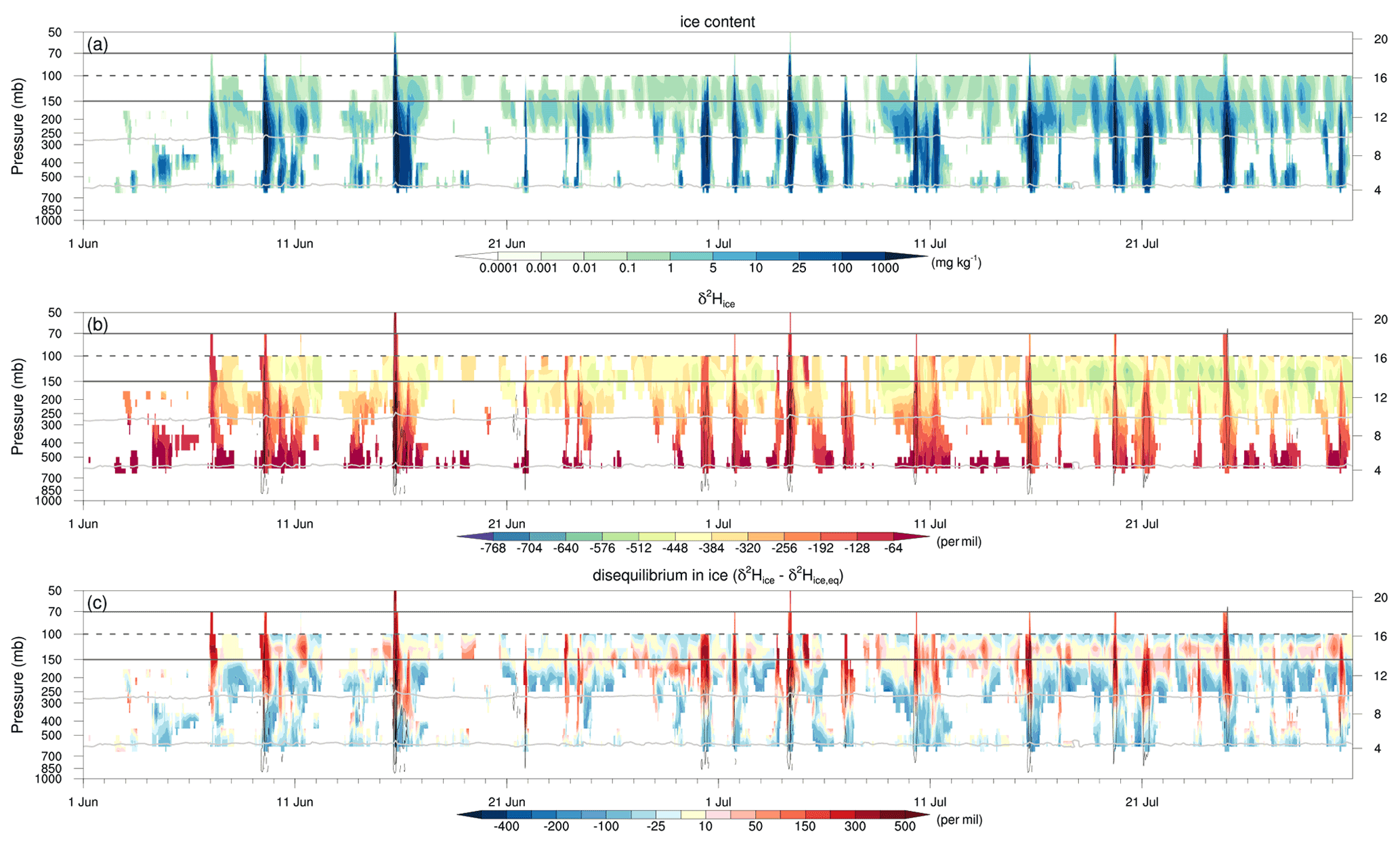
Figure 7The temporal evolution of ice and its isotopic composition for the period from 1 June to 30 July 2016 for the (a) ice content (mg kg−1), (b) δ2H in ice (‰), and (c) disequilibrium in ice (‰) averaged over a small region (14.5–15.5∘ N, 5–6∘ E), indicated by the black boxes in Fig. 6a–d. Variables in all panels are transparent when the domain average ice content values are below 10−4 mg kg−1. As in Fig. 6, the light grey contours denote the liquid, mixed-phase, and ice cloud layers; the dark grey solid contours denote the TTL region; and the dark grey dashed contours denote the approximate tropopause cold point. Black solid (dashed) contours again show the upward (downward) vertical motion but at intervals of 0.1, 0.5, 1, 2, and 5 m s−1.
The isotope signatures of the MCS on 15 June 2016 are not exceptional; instead, they are typical and representative of convective storms in our WAM simulation. Figure 7 shows the temporal evolution of vertical profiles of ice content, δ2H in ice, and disequilibrium in ice for a small 1∘ × 1∘ region (black boxes in Fig. 6a–d) throughout the simulation period of June–July 2016. Multiple convective storms pass through this small region, as revealed by the large amounts of ice that reach into the upper troposphere (Fig. 7a). Each of these convective storms is characterized by high values of δ2H in ice and very positive Δδ2Hice values (Fig. 7b, c). Intermittent periods between convective storms indicate the presence of cirrus clouds with a lower ice content, more depleted ice, and near-zero Δδ2Hice values in the centre of these clouds at ∼150 hPa as well as negative Δδ2Hice values in the lower parts of these clouds (Fig. 7a, b, c). δ2H in vapour does not exhibit a clear signal during the passages of MCSs due to the spatial averaging over both updraughts and downdraughts within MCSs that concur over the 1∘ target region (not shown).
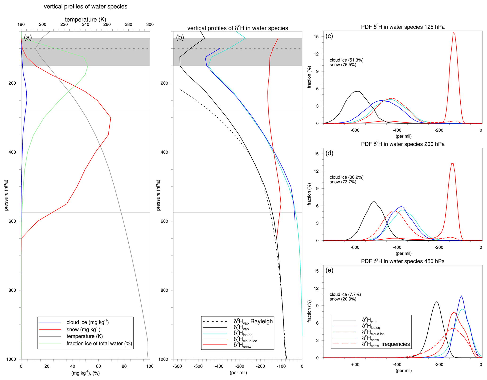
Figure 8Vertical profiles and probability density functions (PDFs) of water species and their isotopic composition in the target region (5–20∘ N, 10∘ W–20∘ E; see black box in Fig. 1) for July 2016. Panels (a) and (b) show vertical profiles of domain average values of (a) temperature, cloud ice, snow, and the fraction of summed cloud ice and snow of total water and of (b) δ2H (‰) in vapour, equilibrium ice, cloud ice, and snow, as indicated by the legend. The black dashed line in panel (b) is δ2H (‰) in vapour as predicted by Rayleigh distillation for moist adiabatic ascent of a saturated air parcel at 1000 hPa with a temperature of 25 ∘C. In panels (c)–(e), the mass-based PDFs of δ2H in water species at 125, 200, and 450 hPa are shown and are complemented by the frequency-based PDFs of snow (red dashed line). The δ2H in cloud ice and snow, shown in panels (c)–(e), is based on grid points with cloud ice and snow content mg kg−1. The fractions of these grid points with respect to all grid points at the respective levels are stated in the text in these panels.
4.2 A statistical analysis
In this section, we proceed to a statistical analysis of water and its isotopic composition in the WAM region of interest (5–20∘ N, 10∘ W–20∘ E; see the black box in Fig. 1) for July 2016. The remainder of this study uses the model output for this region of interest and specific period. The choice to focus on this 1-month period only instead of the full 2-month simulation period aims to circumvent the potential influence of systematic differences in stable water isotope signals before and after the monsoon onset (Risi et al., 2008b) and the gradual depletion of stable water isotopes during the progress of the monsoon (Risi et al., 2010b); see also Fig. 2h. Figure 8a shows the vertical profiles of various water species horizontally averaged in the region of interest. Note that we consider cloud ice and snow separately here as an exception to all other analyses in this study. Cloud ice content reaches a maximum of ∼4.4 mg kg−1 near 250 hPa, while snow content attains an about 10-fold larger maximum of ∼70 mg kg−1 near 300 hPa. The fraction of summed cloud ice and snow in total water is largest between 100 and 200 hPa and exceeds 50 % in this layer. Figure 8b shows the corresponding vertical profiles of δ2H values in vapour, cloud ice, and snow. δ2H in vapour (black line) decreases with height approximately following Rayleigh distillation until an altitude near 400 hPa and transits above away from the Rayleigh regime with increasing δ values with height for p<150 hPa (where p denotes pressure), which is consistent with previous model studies and observations (Kuang et al., 2003; Bony et al., 2008; Steinwagner et al., 2010; Randel et al., 2012). The isotopic composition of vapour reaches a minimum near the bottom of the TTL at 150 hPa, well below the cold-point tropopause near 100 hPa (Fig. 8a), with δ values near −590 ‰. This value is roughly in agreement with the −650 ‰ estimates from the Atmospheric Trace Molecule Spectroscopy (ATMOS) measurements in November 1994 (Kuang et al., 2003), the −650 ‰ from satellite-based measurements across the tropics (Randel et al., 2012), minimum values between −600 ‰ and −400 ‰ from aircraft measurements in the North American monsoon (Hanisco et al., 2007), values between −650 ‰ and −400 ‰ from a flight campaign out of Costa Rica in August 2007 (Sayres et al., 2010), and the −530 ‰ from single-column model simulations in a tropical environment (Bony et al., 2008). Ice that would form under equilibrium fractionation from local vapour (turquoise line) demonstrates a similar profile to that of δ2H in cloud ice from the model output (blue line; Fig. 8b). These similar vertical profiles reflect the in situ formation of small ice crystals with negligible fall velocities. In contrast, the vertical profile of δ2H in snow (red line; Fig. 8b) deviates substantially and shows roughly constant δ values with height near −150 ‰. We hypothesize that this profile results from strong vertical transport of the frozen condensate in convective regions.
To provide a more detailed picture of the isotopic composition of the water species, we consider their mass-based probability density functions at three specific pressure levels (Fig. 8c, d, e). Consistent with our earlier note, the distributions of δ2H in cloud ice from model output are close to the local equilibrium values at all three levels, illustrating the in situ formation of small, suspended ice crystals under equilibrium fractionation. The mass-based probability density function of δ2H in snow (red solid lines in Fig. 8c–e) shows a bimodal distribution at 125 and 200 hPa, with a primary peak near −130 ‰ and a secondary peak near −425 ‰ hPa. The probability density functions based on occurrence frequencies (red dashed lines in Fig. 8c–e) show that the enriched peak results from relatively few occurrences, in contrast to the depleted peak that corresponds to large occurrence frequencies. These distributions suggest that the convective lofting of large amounts of enriched snow occurs in sparse updraughts, while much lower amounts of more depleted snow develops through the aggregation of ice crystals formed in situ in widespread cirrus. At 450 hPa, both the mass- and frequency-based distributions of snow are shifted towards more depleted δ2H values compared with equilibrium ice, as a result of the sedimentation of relatively depleted snow from higher altitudes (Fig. 8e).
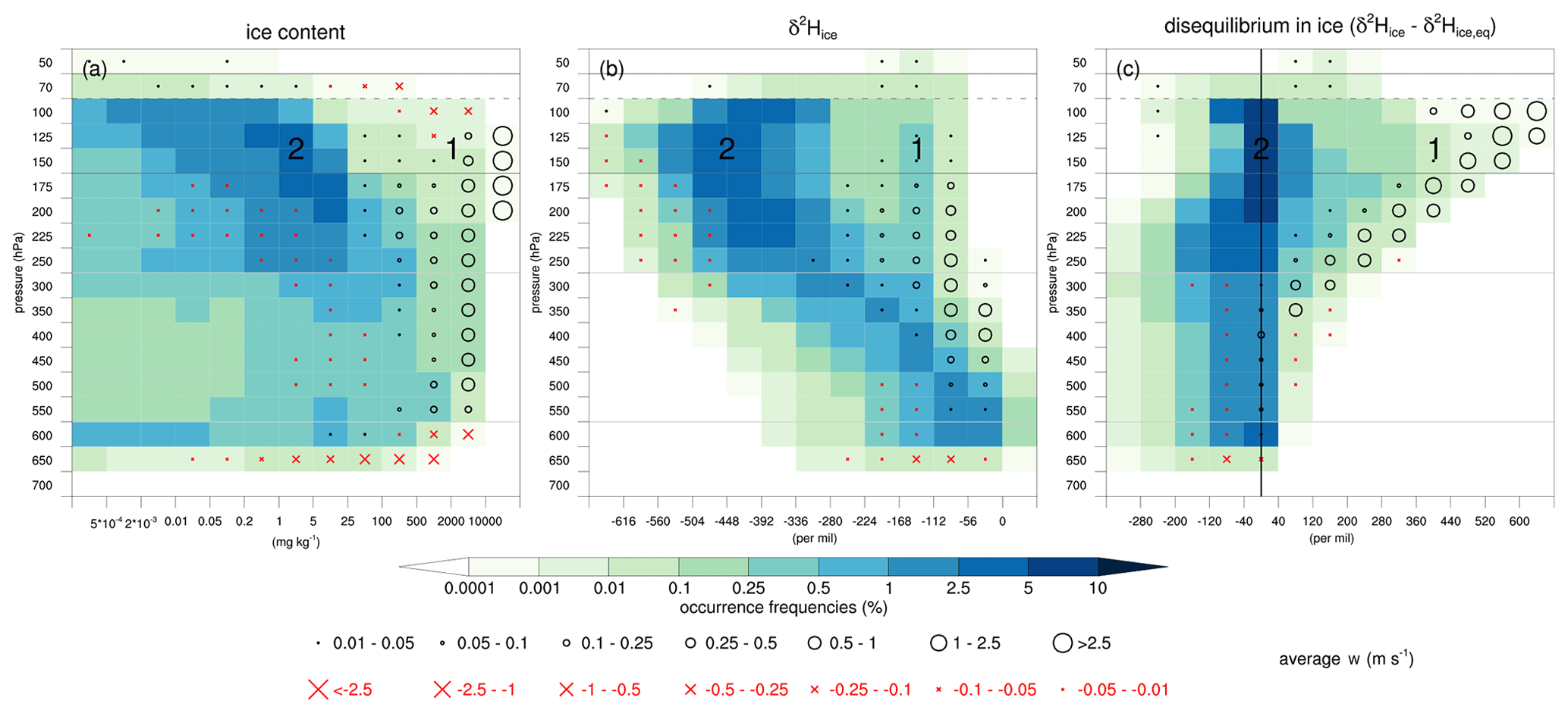
Figure 9Frequency distribution of ice and its isotopic composition across pressure levels in the region of interest for July 2016. Frequency occurrences of (a) ice content (mg kg−1), (b) δ2H in ice (‰), and (c) disequilibrium in ice (‰) are based on grid points with ice content mg kg−1. Black circles (red crosses) denote the positive (negative) average vertical motion for the corresponding bins, as indicated by the legend, and are only plotted for bins where the frequency occurrences exceed 10−4 %. The labels (1) and (2) in the panels refer to the processes discussed in the text.
Consistent with the case study, this analysis highlights two different formation pathways of ice that we will further investigate. Figure 9 shows the frequency distribution of ice and its isotopic composition on pressure levels from 50 to 700 hPa with the average vertical motion for each individual bin overlaid. For clarity, we consider the sum of cloud ice and snow again here. Ice clouds occur most frequently in the upper troposphere (125–250 hPa) with ice content between 0.2 and 25 mg kg−1 (Fig. 9a). Most ice gradually depletes with altitude (Fig. 9b). Ice in this regime forms in situ under equilibrium fractionation as indicated by the near-zero disequilibrium in ice (Fig. 9c), especially in the upper troposphere (100–200 hPa). These high frequencies in the distribution are suggestive of depositional growth and the aggregation of ice crystals formed in situ in vast cirrus shields. A part of the ice cloud distribution differs remarkably from this regime. Few regions with relatively low occurrence frequencies have very large ice content amounts (>2000 mg kg−1) associated with strong convective updraughts with an average upward motion >1 m s−1 (Fig. 9a). This part of the distribution also emerges as relatively enriched ice for p<400 hPa that clearly deviates from the in situ formation regime, indicative of convective lofting of enriched ice (Fig. 9b). Indeed, the distribution of the disequilibrium in ice demonstrates occurrences with increasingly larger positive Δδ2Hice values with height, exceeding +600 ‰ in the lower TTL (100–125 hPa; Fig. 9c). These positive Δδ2Hice values coincide with strong upward motion in the lower parts of these positive values. Thus, the frequency distribution in Fig. 9 demonstrates convectively lofted enriched ice and ice formed in situ under equilibrium fractionation (labels “1” and “2” in Fig. 9 respectively). These results show large similarities to those from Blossey et al. (2010) (their Fig. 6). In addition, Fig. 9c also shows that a substantial part of the distribution falls in the range of negative Δδ2Hice values near −200 ‰ and even down to ‰. These signals stem from sedimenting ice that formed at higher altitudes and is relatively depleted with respect to local vapour conditions. These negative Δδ2Hice values appear from the upper troposphere to the melting level (200–600 hPa) and, thus, include sedimentation of ice from both cirrus clouds in the upper troposphere and convective clouds in the mixed-phase cloud layer. We also observe weak downward motion in the 300–600 hPa pressure layer for moderately negative Δδ2Hice values between −40 ‰ and −120 ‰, reflecting the signatures of convective downdraughts. The next section systematically investigates the relationship between vertical motion and the isotope signals in ice and water vapour to further identify the relevant processes in convective updraughts and downdraughts.
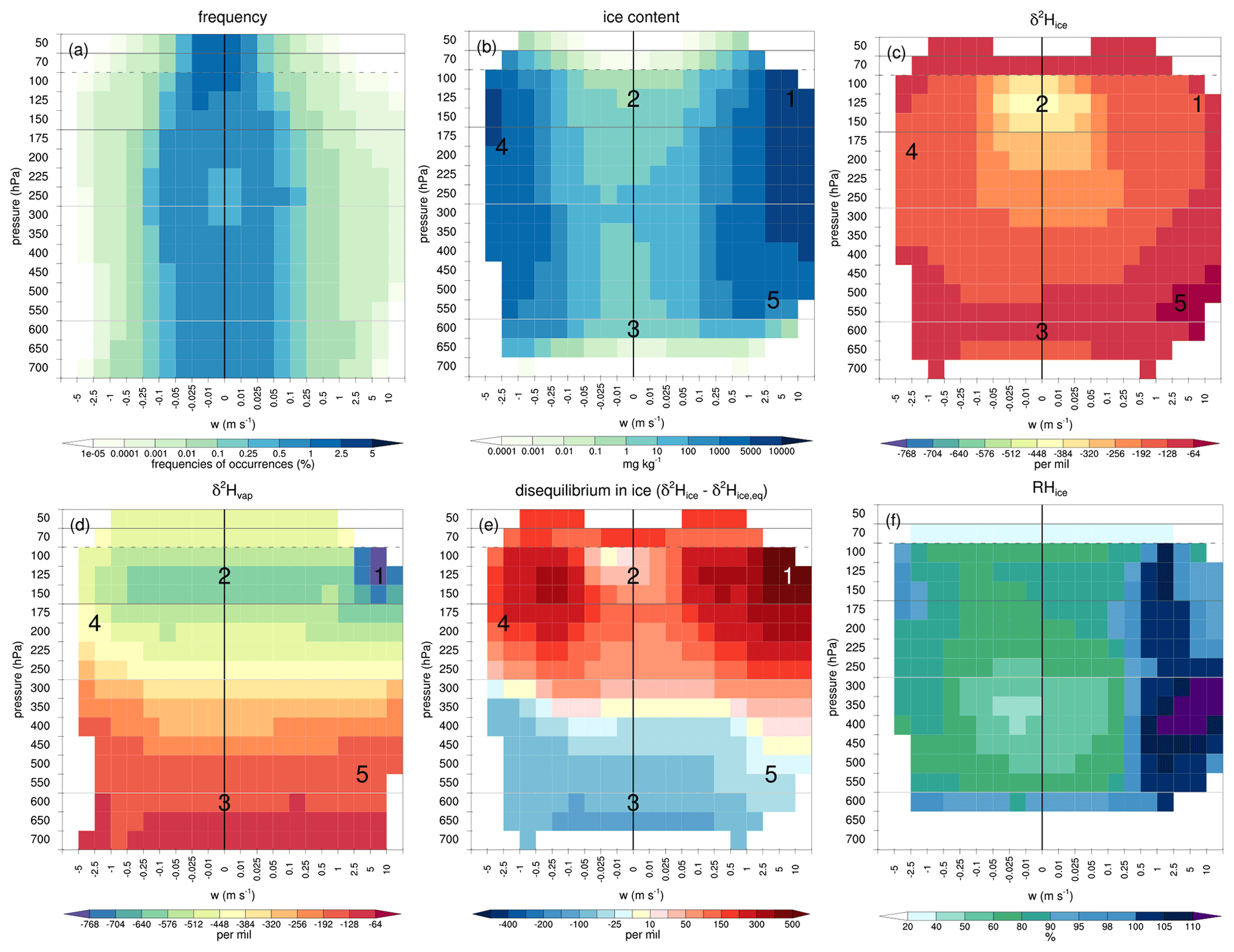
Figure 10Frequency distribution and isotopic composition of water species as a function of vertical motion across pressure levels in the region of interest for July 2016 for (a) frequency occurrences (%), (b) ice content (mg kg−1), (c) δ2H in ice (‰), (d) δ2H in vapour (‰), (e) disequilibrium in ice (‰), and (f) relative humidity with respect to ice (%). Values in panels (b)–(f) are transparent when the frequency occurrences are below 10−5 %, and they are also transparent in panels (c) and (e) if the average ice content falls below 10−4 mg kg−1. Note the irregular intervals and asymmetric distribution of the vertical motion bins, as indicated on the x axes.
4.3 Convective updraughts and downdraughts
Figure 10 presents the characteristics of water species and their isotopic compositions as a function of vertical motion across pressure levels. For each bin, we retrieve the occurrence frequencies, average ice content, δ2H in ice, δ2H in vapour, disequilibrium in ice, and relative humidity over ice (RHice) (Fig. 10a, b, c, d, e, f). The distribution is centred near zero vertical motion and displays some asymmetry with slightly enhanced frequencies of weak downward motion and an extended “tail” towards strong upward motion (Fig. 10a). Both strong updraughts and downdraughts contain large amounts of ice that is relatively enriched compared with more depleted ice in regions with weak vertical motion (Fig. 10b, c). The disequilibrium in ice exceeds 500 ‰ in the updraughts and 300 ‰ in weaker downdraughts near 125–150 hPa (Fig. 10e). The isotopic composition of vapour at these altitudes is very depleted in strong updraughts ( ‰) and very enriched in downdraughts ( ‰) at slightly lower altitudes near 175 hPa (Fig. 10d). This large range in δ2H in vapour corresponds to our earlier findings based on the MCS case study (Sect. 4) and is corroborated by the month-long statistical analysis here. Moreover, this large range of δ2H in vapour is consistent with observations (Webster and Heymsfield, 2003; Hanisco et al., 2007; Sayres et al., 2010). Here, we provide evidence that these large fluctuations are directly related to vertical motion and the moist processes that take place in deep convection – that is, condensation and deposition in updraughts and sublimation in downdraughts.
The information in Fig. 10 also serves perfectly to illustrate the five key processes postulated in Sect. 4.1; see the labels 1–5 in Fig. 10. We briefly reiterate these five processes based on the statistical analysis. (1) Convective ice lofting corresponds to the right-hand side of the distribution (i.e. strong updraughts) and is characterized by large ice content amounts (>5000 mg kg−1), relatively high δ2Hice values ( ‰), very large positive Δδ2Hice values (>500 ‰), and very low δ2Hvap values ( ‰) as a result of the preferential condensation and deposition of heavy isotopes in these updraughts. In contrast, (2) in situ formation of ice under equilibrium fractionation in regions with weak or negligible vertical motion has a moderate ice content (0.1–10 mg kg−1), relatively depleted ice ( ‰), and near-zero Δδ2Hice values. (3) In lower parts of the troposphere with weak vertical motion, we note the signatures of sedimenting and sublimating ice that formed at higher altitudes and is relatively depleted with respect to the local vapour conditions, which is reflected by moderately negative Δδ2Hice values near −100 ‰, especially near the melting level at ∼600 hPa. (4) In upper-tropospheric regions of strong convective downdraughts, on the left-hand side of the distribution, non-fractionating sublimation of enriched ice enriches the ambient vapour, with δ2H values that are almost twice as high as in regions of convective updraughts at similar altitudes. Sublimation in downdraughts is likely to occur as the RHice falls below 100 % (Fig. 10f). (5) In mid-tropospheric regions of moderate upward motion, liquid water freezes just above the 0 ∘C isotherm, which is reflected by weakly negative Δδ2Hice values near −25 ‰. As already explained in Sect. 4.1, this signal stems from the lower equilibrium fractionation factor of condensation than that of vapour deposition, resulting in liquid water being isotopically lighter than ice that would form directly from the vapour phase. This analysis demonstrates that the new variable introduced in this study, disequilibrium in ice (Δδ2Hice), is a particularly useful measure to investigate the processes related to the formation and decay of ice clouds. We elaborate on this concept in a theoretical perspective on this variable in Appendix A.
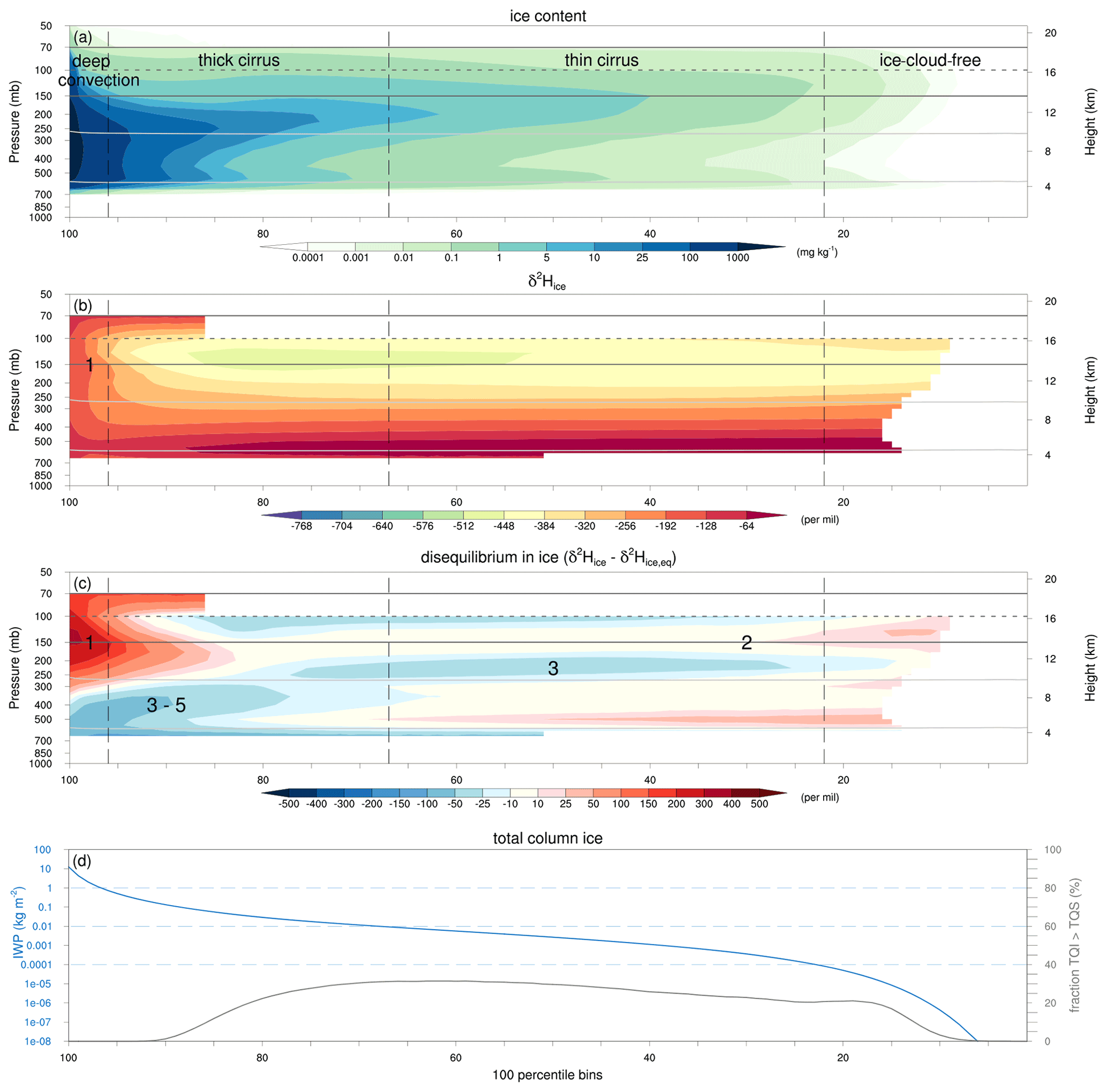
Figure 11Vertical distribution of ice and its isotopic composition as a function of IWP in the region of interest for July 2016. Vertical profiles show the (a) ice content (mg kg−1), (b) δ2H in ice (‰), (c) disequilibrium in ice (‰), and (d) IWP amounts (blue; kg m−2) as well as the fraction of grid points with TQI > TQS (%), constructed using 100 percentile bins ranked on IWP; see the text for details. δ2H in ice and disequilibrium in ice values are transparent when the average ice content is below 10−4 mg kg−1.
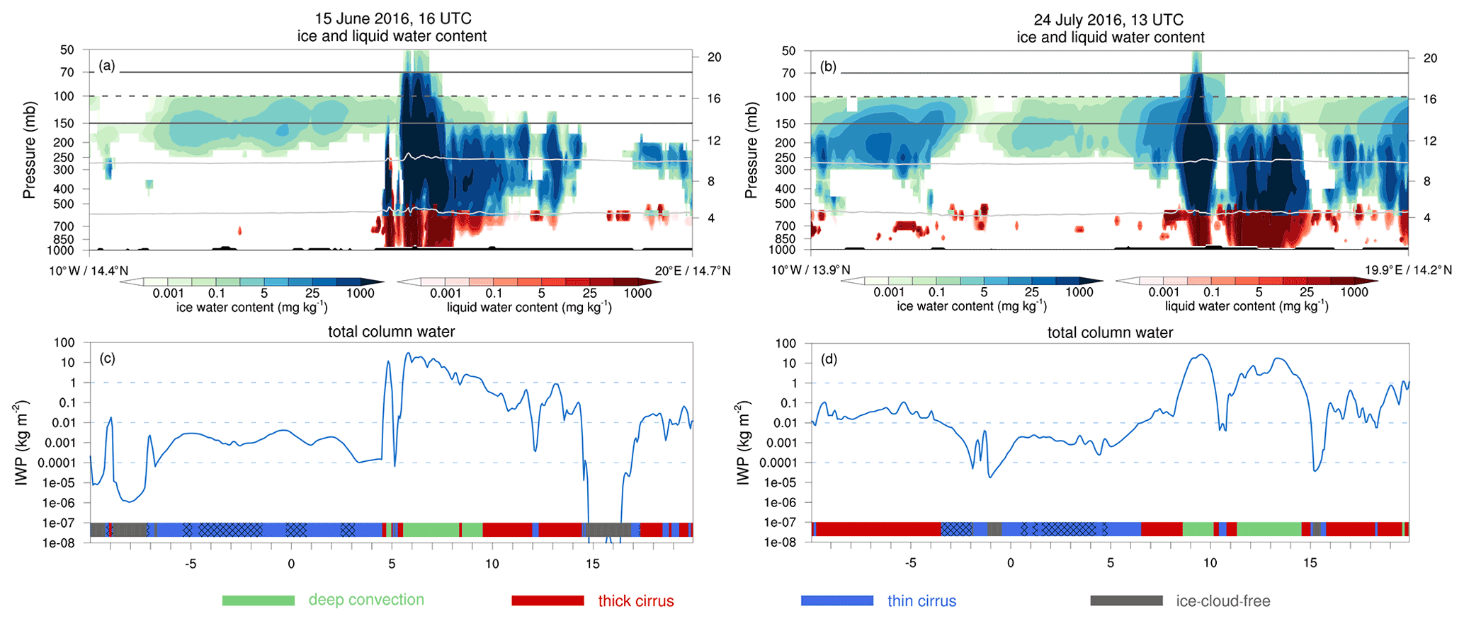
Figure 12Illustrative examples of the different ice cloud regimes. Panels (a) and (b) show the vertical cross sections in a zonal direction with ice water content in blue (mg kg−1) and liquid water content in red (mg kg−1) for 15 June 2016 at 16:00 UTC and 15 June 2016 at 16:00 UTC respectively; panels (c) and (d) show the corresponding IWP amounts (blue, kg m−2) for the same respective dates and times. The horizontal lines in panels (c) and (d) indicate the thresholds applied to IWP (light blue) to distinguish the different ice cloud regimes. The coloured bars in the lower parts of panels (c) and (d) detail the ice cloud regimes as indicated by the legend below, and the black hatching of the blue bars indicates thin-cirrus regions where TQI > TQS; see the text for details.
5.1 Ice cloud classification method
Section 4 already described different types of ice clouds and their associated isotope signatures. To objectively classify regions with different types of ice clouds, we use total column ice, hereafter referred to as ice water path (IWP). IWP is computed by the sum of total column cloud ice (TQI) and total column snow (TQS). Figure 11 displays the vertical distributions of ice content, δ2H in ice, and disequilibrium in ice in 100 percentile bins of IWP ranked from the largest amounts on the left to the lowest amounts on the right, following Gasparini et al. (2019) (their Fig. 1). On the left, for high IWP, we clearly recognize the signatures of deep convection with a very large ice content up to the tropopause cold point, transitioning into a cirrus shield with a lower ice content towards lower IWP percentiles, and ending with an ice-cloud-free region on the right (Fig. 11a). The isotope signals in ice correspond to these suggested cloud types. Deep convective clouds are characterized by very enriched ice and positive disequilibrium in ice in the ice-phase layer ( ∘C; Fig. 11b and c, label “1”). Cirrus clouds show, on average, near-zero Δδ2Hice values (Fig. 11c, label “2”). Underneath the cirrus shield we observe small negative Δδ2Hice values near −25 ‰ within the ice-phase layer ( ∘C), reflecting the sedimentation and sublimation of ice particles (Fig. 11c, label “3”). Negative disequilibrium in ice in the mixed-phase cloud layer between the 80th and 100th percentile range reflects a combination of (3) sedimentation and sublimation of ice, (4) downward transport of ice in convective downdraughts, and (5) a minor influence of freezing liquid water in convective updraughts (Fig. 11c, labels “3–5”). The distribution of ice in Fig. 11 can also be interpreted as liquid-origin ice from freezing and deposition in convective updraughts on the left and in situ ice formed directly from the vapour phase under the influence of gravity wave activity or uplift above convective cells further to the right (Krämer et al., 2016).
Following Sokol and Hartmann (2020), Nugent et al. (2022), and Turbeville et al. (2022), we use IWP to distinguish three different categories of ice cloud regimes:
-
deep convection, IWP >1 kg m−2;
-
thick cirrus, kg m−2;
-
thin cirrus, kg m−2.
In addition to these three ice cloud regimes, we consider regions with IWP <0.0001 kg m−2 to be “ice-cloud-free”. Figure 12 shows two examples at different time instances to demonstrate the functionality of using IWP as proxy for different ice cloud regimes. Deep convective regions have a very large ice content (and liquid water content) that reaches from the middle to the upper troposphere, classified as “deep convection” (see green bars in Fig. 12c and d). Regions labelled as “thick-cirrus” clouds manifest as a combination of convective outflow, juvenile convection, and remnants of convective storms. Extensive regions with relatively low ice content in the upper troposphere are classified as “thin cirrus”. Approximately 30 % of these thin-cirrus regions have larger TQI than TQS; see the black hatching in the blue cirrus labels in Fig. 12c and d and the grey line in Fig. 11d. This subcategory is used in a later analysis to separate atmospheric columns with predominantly suspended ice crystals from those where precipitating snow dominates IWP.

Figure 13The statistical distribution and averages of ice and its isotopic composition for the 50–700 hPa pressure range in the region of interest in July 2016. Boxes and whiskers indicate the 10th, 25th, median, 75th, and 90th percentiles and dots represent the averages of the (a) ice content (mg kg−1), (b) δ2H in ice (‰), and (c) disequilibrium in ice (‰) for the ice cloud regimes, as indicated by the legend. The numbers in the text indicate the fractions of grid points in each ice cloud regime. The statistical distribution is based on grid points with an ice content mg kg−1, whereas the averages are based on all grid points within the region of interest for the respective ice cloud regimes.
5.2 Isotope signals in convective and cirrus clouds
Figure 13 shows vertical profiles of the statistical distributions and averages of ice content, δ2H in ice, and disequilibrium in ice for the three ice cloud regimes. The statistical distribution is based on grid points with ice content mg kg−1, whereas the average values are derived from all grid points in the corresponding ice cloud regimes. The three ice cloud regimes deep-convective, thick-cirrus, and thin-cirrus clouds correspond to 3.8 %, 28.7 %, and 45.2 % of the grid points within the region of interest respectively, while the remaining 22.3 % belong to ice-cloud-free regions. By definition, deep convection is characterized by very large ice content amounts (∼1 g kg−1) throughout the middle and upper troposphere (Fig. 13a). Around the cold-point tropopause near 100 hPa, the average ice content is far outside the 10th–90th percentile range, reflecting rare overshooting convection that brings very large amounts of ice to these high altitudes. Thin cirrus displays a relatively low ice content in the upper troposphere, peaking around ∼200 hPa with average values near 2 mg kg−1, whereas thick cirrus exhibits a moderate ice content, near 25 mg kg−1 throughout the middle and upper troposphere.
Average δ2H in ice within deep convection demonstrates roughly constant δ values with height, near −140 ‰ (Fig. 13b). In the upper troposphere, ice in deep convection is very enriched compared with ice in thick and thin cirrus (Fig. 13b). For example, the average δ2H in ice at 200 hPa is −151 ‰ in deep convective clouds compared with −321 ‰ and −390 ‰ for thick and thin clouds respectively. In the middle troposphere, this pattern reverses somewhat, and ice in deep convective regions is on average slightly more depleted than ice in thick- and thin-cirrus clouds. The transition of very enriched ice in the upper troposphere to slightly depleted ice in the middle troposphere in deep convective clouds compared with thick- and thin-cirrus clouds also clearly emerges in vertical profiles of disequilibrium in ice (Fig. 13c). Average Δδ2Hice values in deep convection range from over +300 ‰ in the upper troposphere to almost −90 ‰ in the middle troposphere. In contrast, average Δδ2Hice values in thin cirrus are close to zero throughout the troposphere, consistent with ice formed in situ under equilibrium fractionation, which is in agreement with earlier findings in Sect. 4.
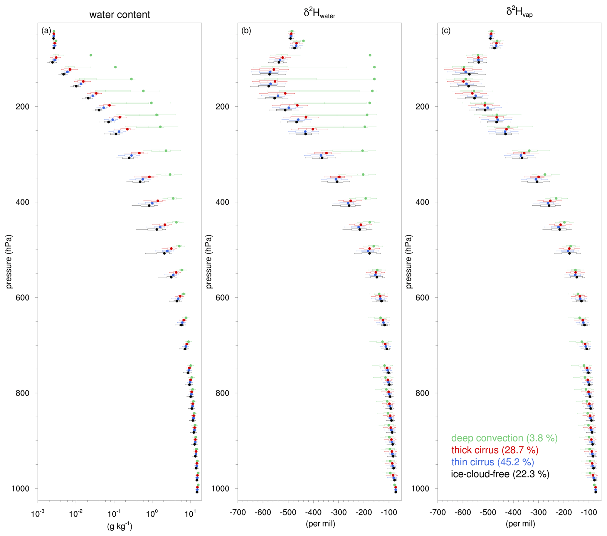
Figure 14As in Fig. 13 but for the (a) total water content (g kg−1), (b) δ2H in total water (‰), and (c) δ2H in vapour (‰) for the 50–1000 hPa pressure range. In addition, the information on the ice-cloud-free regime is included in black.
Figure 14 shows the vertical profiles of the statistical distributions and averages of total water content, δ2H in total water, and δ2H in vapour for the three ice cloud regimes as well as for ice-cloud-free regions. Here, total water is defined by the sum of vapour, cloud ice, snow, cloud water, and rain, hereafter referred to as “water” for simplicity. In the upper troposphere, deep convective regions contains about 1–2 orders of magnitudes more water than thick-cirrus, thin-cirrus, and ice-cloud-free regions (Fig. 14a). δ2H in water in deep convection is much more enriched in the upper troposphere (p<500 hPa) and slightly more depleted in the lower troposphere (p>500 hPa) than in other cloud regimes (Fig. 14b). These profiles show how vertical transport by deep convection acts to redistribute the isotopic composition of water throughout the troposphere. Average δ values in vapour are relatively similar in all four ice cloud regimes (Fig. 14c). Closer inspection shows that average δ2Hvap in deep convection is slightly more enriched near 300 hPa and slightly more depleted in the lower troposphere (p>600 hPa) compared with δ2Hvap in ice-cloud-free regions. This finding is consistent with previous studies which suggested that deep convection enriches vapour at the approximate level of convective outflow and depletes low tropospheric vapour as a result of depleted upper-tropospheric air entrained in convective downdraughts and rain evaporation (Bony et al., 2008; Risi et al., 2008a; Blossey et al., 2010; Randel et al., 2012). In the upper troposphere (150–300 hPa), the distribution of δ2H in vapour shows a larger spread in deep convective regions compared with thick-cirrus, thin-cirrus, and ice-cloud-free regions. This may stem from the fact that deep convection has a much lower sample size than the other ice cloud regimes, but it more likely reflects the strong opposing effect of moist processes in updraughts and downdraughts on the vapour isotopic composition, as shown in Sect. 4.3.
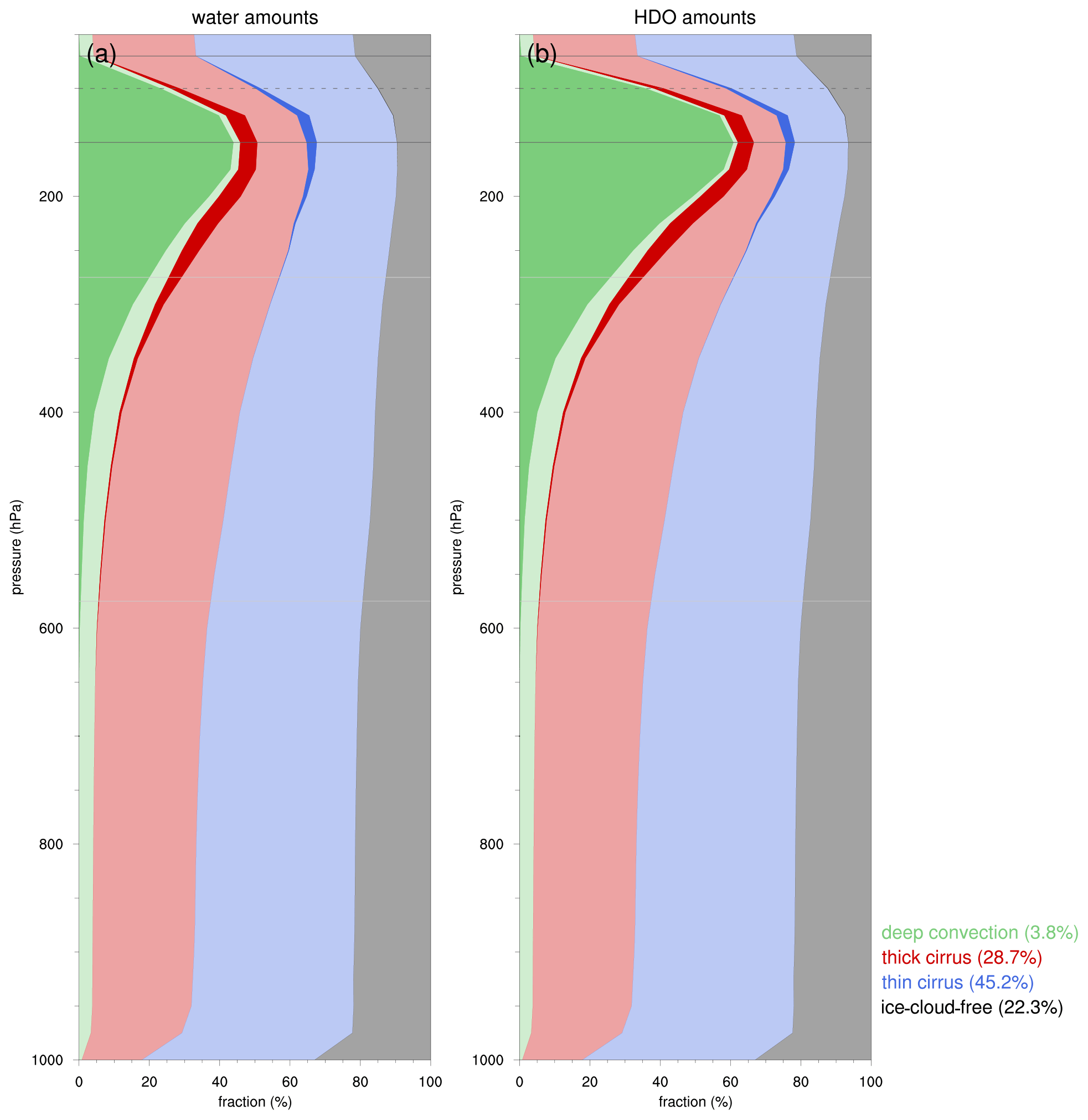
Figure 15Total water amounts partitioned over the four ice cloud regimes in the region of interest in July 2016. The colours show the (a) total water and (b) total deuterated water (HDO) amounts within the four different ice cloud regimes, as indicated by the legend. Opaque colours represent water in the ice phase, and transparent colours represent water in the vapour and liquid phases. The numbers in the legend indicate the fractions of grid points in each of the different ice cloud regimes.
To provide context for the analysis above, we present the total water amounts that each ice cloud regime holds in the region of interest in July 2016. Figure 15 shows the partitioning of total water and HDO across the four ice cloud regimes. Opaque colours correspond to ice, and transparent colours correspond to water in the vapour and liquid phases. In the lower troposphere (p>500 hPa), the total water is proportionally distributed across the different ice cloud regimes. In the upper troposphere and the lower TTL (125–200 hPa), deep convective regions contain more than 40 % of the total water (Fig. 15a). This points to a disproportionally large influence of deep convection on TTL water, considering that convective regions only constitute about 3.8 % of the atmosphere in our model simulations. Fractions of heavy deuterated water (HDO) in convective regions are even larger and reach ∼60 % at these high altitudes (Fig. 15b). Almost all water and deuterated water in deep convection in this part of the atmosphere consists of ice (opaque colours in Fig. 15a and b). Compared with deep convective regions, ice fractions in the mixed and cirrus clouds are much lower, and vapour contributes most to the total water amounts. These findings suggest a key role of deep convection in modulating the lower TTL water and its isotopic composition through convective ice lofting.

Figure 16Frequency distribution of the isotopic composition of vapour and average vertical motion in the region of interest in July 2016. Frequency occurrences (%) of δ2H in vapour for the (a) deep-convective and (b) thin-cirrus with TQI > TQS ice cloud regimes. Black circles (red crosses) denote the positive (negative) average vertical velocity (m s−1) for the corresponding bins, as indicated by the legend, and are only plotted if frequency occurrences exceed 10−4 %.
5.3 Water vapour isotope signals in convective vs. large-scale circulation regimes
To assess the impact of vertical motion on the isotopic composition of water vapour in different ice cloud regimes, we construct the frequency distribution of δ2H in vapour overlaid with the average vertical motion for regions with deep convection and thin cirrus (Fig. 16). Note that the thin-cirrus clouds in this analysis only contain the regions where TQI > TQS (12.3 % of all grid points) to remove atmospheric columns where snow particles dominate suspended ice crystals. In the upper troposphere, the range in δ2H values in vapour within deep convection is much larger than that in thin-cirrus regions and reaches from about −850 ‰ to −350 ‰ (Fig. 16a). Very depleted vapour is characterized by strong upward motion, whereas very enriched vapour is associated with strong downward motion. For example, in the lower TTL, at 125 hPa, very depleted vapour with δ2H values between −832 ‰ and −768 ‰ coincides with an average upward motion of 2.1 m s−1, whereas very enriched vapour between −384 ‰ and −320 ‰ at this altitude experiences an average downward motion of −0.9 m s−1. These findings are in line with the discussion in Sect. 4 and are explicitly shown here to occur within deep convective regions. The observed pattern reverses in the lower troposphere at p>500 hPa where relatively enriched (depleted) vapour is associated with upward (downward) motion. Likely, this effect results from the transport of enriched vapour in updraughts to higher altitudes (which dominates the depletion of vapour by the preferential condensation and deposition of heavy isotopes at these lower altitudes) and the transport of depleted vapour in downdraughts to lower altitudes, further depleted by rain evaporation or equilibration with falling raindrops.
In thin-cirrus regions, the relationship between the isotopic composition of vapour and vertical motion demonstrates a reversed pattern in the upper troposphere compared with deep convection. Relatively depleted vapour in thin cirrus is associated with weak downward motion ( m s−1) between 125 and 250 hPa, whereas enriched vapour goes along with weak upward motion (∼0.04 m s−1) between 175 and 350 hPa (Fig. 16b). Most likely, these signatures reflect the vertical transport of depleted vapour from higher altitudes by large-scale subsidence and enriched vapour from lower altitudes by large-scale upwelling. Thus, isotope signals in vapour differ remarkably between regions dominated by convective activity and the large-scale circulation. Fractionation during phase changes dominates the isotope signals in upper-tropospheric vapour in regions of deep moist convection, while the direct vertical transport of vapour is of first-order importance in regions dominated by the large-scale circulation.
This study investigated the atmospheric processes related to tropical ice clouds and deep convection using regional convection-permitting model simulations in the West African monsoon (WAM) for June–July 2016. The motivation of this work is to better understand these processes using stable water isotope tracers. This work adds three important aspects to previous studies. (1) Whereas previous stable water isotope modelling studies used conceptual frameworks, Lagrangian trajectory calculations, single-column models, idealized large-eddy simulations, idealized two-dimensional cloud-resolving models, and GCM simulations (Dessler and Sherwood, 2003; Dessler et al., 2007; Bony et al., 2008; Blossey et al., 2010; Sayres et al., 2010; Eichinger et al., 2015), we use, for the first time, regional convection-permitting model simulations constrained by actual meteorological conditions. (2) Building upon observational and modelling insights into the formation and decay of tropical ice clouds (Krämer et al., 2016; Urbanek et al., 2017; Gasparini et al., 2019, 2021), we present an integrated view on these processes based on stable water isotope information. (3) We contribute to the long-standing debate on processes that modulate the tropical tropopause layer (TTL) water budget and show, consistent with previous observations and modelling efforts (Moyer et al., 1996; Kuang et al., 2003; Steinwagner et al., 2010; Bolot and Fueglistaler, 2021), that deep convection influences the TTL water vapour isotopic composition through the moist processes that take place in convective updraughts and downdraughts.
First, we evaluated our regional model simulations by comparing model output from simulations with different resolutions and treatments of convection to observations of isotopes in mid-tropospheric water vapour and monthly precipitation. Our model simulations show a systematic difference to IASI water vapour isotope observations but follow the temporal evolution throughout the simulation period very well. Furthermore, our simulations reasonably represent the spatial distribution of monthly precipitation isotopes compared with GNIP observations. Calculation of root mean square errors showed that the convection-permitting simulation with a horizontal grid spacing of 7 km and 60 model levels outperforms the simulations with parameterized and explicit convection at a horizontal grid spacing of 14 km. For the remaining analysis of tropical ice clouds, we used the convection-permitting simulation with a 7 km horizontal grid spacing. This simulation also represents the different stages in the monsoon evolution as well as the westward movement of mesoscale convective systems (MCSs) over the Sahel very well compared with the GPM IMERG precipitation observations.
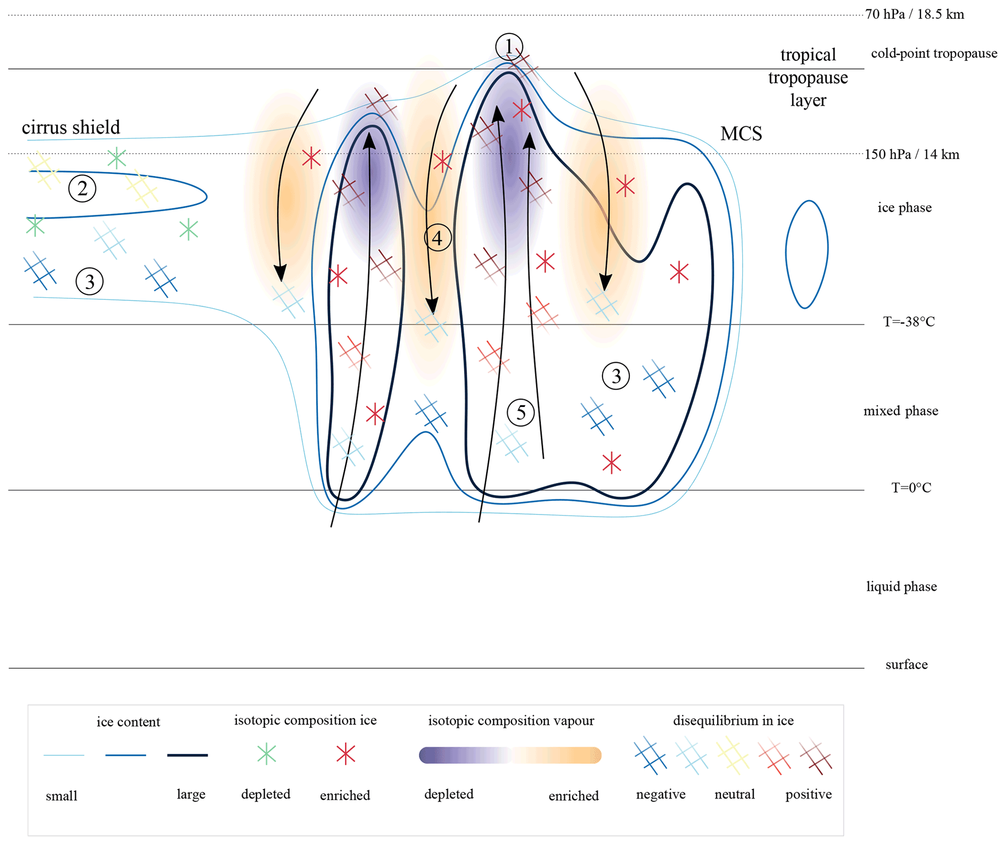
Figure 17Schematic representation of the five key processes related to the formation and decay of tropical ice clouds: (1) convective lofting of very enriched ice along with the isotopic depletion of vapour through the preferential condensation and deposition of heavy isotopes in the updraughts, (2) in situ formation of ice under equilibrium fractionation in cirrus shields, (3) sedimentation and sublimation of ice in the mixed-phase cloud layer of convective systems and underneath cirrus shields, (4) non-fractionating sublimation of ice in convective downdraughts that enriches the environmental vapour, and (5) freezing of liquid water in the lower parts of convective updraughts. These processes are reflected by stable water isotope signals in ice, vapour, and especially the disequilibrium in ice (Δδ2Hice), as indicated by the legend. See the text for details.
A case study of an MCS and a complementary statistical analysis reveal how tropical deep convection modulates the isotopic composition of water vapour and ice. Five key processes could be identified based on isotope information that are related to the formation and decay of tropical ice clouds, as schematically depicted in Fig. 17:
-
Convective updraughts transport enriched ice into the upper troposphere, which goes along with a strong depletion of vapour by the preferential condensation and deposition of heavy isotopes in these updraughts.
-
In contrast, ice in widespread cirrus shields is in approximate isotopic equilibrium with the environmental vapour, suggesting in situ formation of ice under equilibrium fractionation.
-
Sedimentation and sublimation of ice is evident in the mixed-phase cloud layer in convective regions and underneath cirrus shields, as derived from moderately negative disequilibrium in ice.
-
Convective downdraughts go along with non-fractionating sublimation of ice that enriches the environmental vapour in the upper troposphere.
-
Freezing of liquid water above the 0 ∘C isotherm in convective updraughts is reflected by weakly negative disequilibrium in ice as a result of a lower equilibrium fractionation factor of condensation compared with vapour deposition.
Previous studies have addressed several of these processes from a stable water isotope perspective. Risi et al. (2008b) and Bony et al. (2008) pointed to the relevance of convective processes that affect the isotopic composition of water vapour as a result of condensate lofting, rain evaporation, unsaturated downdraughts, and the isotopic exchange between droplets and the tropospheric environment. Bolot et al. (2013) used a conceptual model to address the cloud microphysical processes that affect the water isotopes, such as condensation, freezing, and deposition in convective updraughts. Blossey et al. (2010) showed that sublimation of convectively lofted ice can enrich TTL vapour, while the fractionation of in situ ice formation can lead to the isotopic depletion of TTL vapour. In this study, we present an integral perspective on these ice cloud processes for which the concept of disequilibrium in ice (see Appendix A for more information) appears particularly useful.
Particularly striking is the large variability in the isotopic composition of water vapour in the upper troposphere and lower TTL (100–200 hPa). δ2H values can reach below −800 ‰ in strong convective updraughts and over −400 ‰ in strong convective downdraughts (Figs. 10d, 16a). Previous studies already noted a very large range of δ2H in vapour based on observations at these altitudes (Webster and Heymsfield, 2003; Hanisco et al., 2007; Sayres et al., 2010). We show that moist processes in convective updraughts and downdraughts are responsible for these large fluctuations – that is, vapour depletion due to condensation and deposition in updraughts and vapour enrichment from non-fractionating sublimation of ice in downdraughts. In contrast, water vapour in thin-cirrus regions that are dominated by suspended ice crystals shows an inverse relationship between its isotopic composition and vertical motion. Enriched water vapour is associated with weak ascending motion, whereas depleted vapour is associated with weak descending motion, suggesting a first-order importance of large-scale vertical transport of water vapour. Thus, isotope signals in water vapour can hold important clues as to whether the atmospheric transport is dominated by convection or the large-scale circulation.
Before concluding, we list a few limitations of this work. First, the model simulations used a relatively simplistic one-moment microphysics scheme with two ice species only (suspended ice crystals and sedimenting snow particles), with inherent limitations in the representation of complex cloud microphysical processes. Second, our analysis of tropical ice clouds is based on model simulations with a horizontal grid spacing of 7 km and 60 model levels. Although this resolution is considered appropriate for a convection-permitting set-up, and the simulated MCSs demonstrate a realistic behaviour, the results of this study may be sensitive to the chosen resolution. Third, our study focuses on the WAM region during the period from June to July 2016. Therefore, it is not known to what extent our results are representative for other (monsoon) regions and for other periods. For instance, it is conceivable that deep convection over the Maritime Continent or the Amazon Basin differs in certain aspects from the WAM-related convection investigated in this study.
Overall, this study demonstrates the usefulness of stable water isotopes as a natural tracer of the Earth's water cycle. Based on convective-permitting model simulations for the WAM in 2016, we show that stable water isotopes can reflect different processes related to the formation and decay of tropical ice clouds and that tropical deep convection strongly affects the water vapour isotopic composition in the lower TTL through the moist processes in convective updraughts and downdraughts. These findings can be complemented in future work by using (i) a quasi-global and year-round analysis, (ii) higher-resolution simulations with more advanced ice cloud microphysics schemes, (iii) online trajectories in high-resolution simulations to trace the moist processes and their isotopic signatures along liquid-origin and in situ ice cloud formation pathways, and (iv) budget calculations and forward trajectories to quantify the remote impact of deep convection on the TTL water vapour.
The isotopic disequilibrium in ice with respect to local vapour conditions is a simple measure to quantify how “exotic” the frozen hydrometeors are in a given upper-tropospheric environment (for the reader's convenience the definition from Eq. 1 in the main text is repeated here):
where δ2Hice,eq is obtained as a function of temperature from the local vapour phase δ2Hvap using the Merlivat and Nief (1967) equilibrium fractionation factor also used in the COSMOiso model for ice formation from vapour deposition. The δ2Hice is obtained as a mass-weighted mean from the δ2H of snow and cloud ice water contents. Δδ2Hice reflects (i) vertical displacements due to the transport or sedimentation of frozen hydrometeors, which were formed (at least partly) in an isotopically different environment, and (ii) phase change processes such as water vapour deposition and the sublimation of ice or freezing liquid. Depending on the environmental conditions (updraughts, downdraughts, or no vertical motion), either vertical displacements, phase changes, or a combination of the two are relevant. In the following, we briefly summarize the expected range of numerical values of Δδ2Hice for the five key processes discussed in Sect. 4:
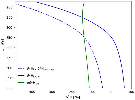
Figure A1Δδ2Hice (green line) obtained from a hypothetical experiment in which ice with the isotope composition δ2Hice is inserted into a totally dry environment, moistened by the sublimation of ice only. Equilibrium ice δ2Hice,eq from this newly formed water vapour is shown by the thick blue line. The δ2Hice profile in this example follows a Rayleigh curve obtained from a moist adiabatic ascent (dashed thick blue line) with T0=30 ∘C at 1000 hPa.

Figure A2The difference between liquid and ice equilibrium fractionation factors. Inspired by Bolot et al. (2013) (their Fig. 1a).
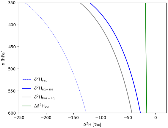
Figure A3Expected Δδ2Hice (green line) when assuming a typical moist adiabatic profile of upper-tropospheric δ2Hvap (dashed thin blue line) with T0=30 ∘C at 1000 hPa. The equilibrium ice formed from this vapour is shown by the thick blue line, and the ice formed from the freezing of locally condensed vapour is shown by the thick grey line.
-
Convective lofting of enriched ice into the upper troposphere.
The upper parts of deep convective updraughts are always associated with large positive Δδ2H values (see Figs. 6h, 7c, 9c and 10e). This reflects the fact that the bulk of the ice with isotope ratio Rice found in these strongly ascending environments has formed at lower altitudes:
with and assuming , where Rvap is the isotope ratio of the local vapour. When treating the hydrometeor categories ice and snow separately (Fig. 8b), it becomes clear that the small ice crystals (cloud ice) that most likely formed recently in the updraught are, on average, in approximate equilibrium with the local vapour Rcloud ice≈αeqRvap (cf. blue line for δ2Hcloud ice and turquoise line for δ2Hice,eq in Fig. 8b). The larger snow hydrometeors, however, are much more enriched than the ice that would form from local vapour at altitudes with p<400 hPa (cf. red line for δ2Hsnow and turquoise line for δ2Hice,eq in Fig. 8b), indicating that the bulk of this snow is transported upward by strong ascending motion from lower altitudes. The Δδ2Hice induced by convective lofting can amount to a maximum of 400 ‰, when considering the range of δ2Hice,eq values in the troposphere (i.e. ice formed at 600 hPa that is transported up to 150 hPa). Local variability, however, can lead to much larger positive Δδ2Hice values, as shown in Figs. 9c and 10e, with values >600 ‰ between 100 and 150 hPa. This can be explained by the excessive depletion of heavy isotopes in very strong convective updraughts, leading to isotopic compositions of vapour below −750 ‰ in the upper core regions of the updraughts, resulting in Δδ2Hice values well above 400 ‰ (Figs. 9c; 10d, e).
-
In situ ice formation under equilibrium fractionation.
In this case, Rice≈αeqRvap; hence, Δδ2Hice≈ 0, assuming bulk equilibrium between vapour and ice with slight variations of ±10 ‰ (see Fig. 6h, 7c, 9c, and 11c), which may be due to (1) turbulent entrainment or detrainment of ice in the upper-tropospheric environment or (2) non-equilibrium fractionation in supersaturated environments.
-
Sedimentation and sublimation of ice in the mixed-phase cloud layer of convective systems and the lower parts of cirrus shields.
Sedimentation leads to a slow descent of the large ice particles. If they formed at higher altitudes, e.g. from aggregation and water vapour deposition on in situ formed ice, then
again assuming , which leads to Δδ2Hice<0. Sedimentation in the upper troposphere can, in principle, lead to Δδ2Hice values as low as −400 ‰ if snow formed at the level of the δ2Hvap minimum at about 150 hPa and sedimented down to the melting level at about 600 hPa following the same rationale as for process 1 (see Fig. 8b). However, minimum values of about −200 ‰ are typically observed in upper-tropospheric environments with weak vertical winds below cirrus shields (at about 200 hPa) or just above the melting level (see Figs. 6h, 7c, 9c, and 10e). This is consistent with the observation that snow formed in the upper troposphere from in situ ice usually sublimates completely in the upper troposphere. The effect of sublimation on Δδ2Hice is discussed below.
-
Convective downdraughts in which ice sublimates.
The effect of sublimation cannot be directly quantified without additional information about sublimation fluxes. Nevertheless, the maximum impact of sublimation on Δδ2Hice can be estimated by choosing the extreme case of ice sublimation into a totally dry environment. As sublimation is assumed to be non-fractionating, Rvap=Rice; thus,
which, when substituting this relation into Eq. (A1) and using δ2Hice instead of Rice, gives
If we assume a typical upper-tropospheric δ2Hice vertical profile, such as shown in Fig. A1, we find Δδ2Hice values between −140 ‰ and −100 ‰ (green line in Fig. A1).
Typically, the background air in the upper troposphere is not totally dry, as assumed in this idealized example; therefore, the Δδ2Hice in an environment with sublimation will be less negative and will depend on the pre-existing specific vapour content, the sublimation flux, and δ2Hvap. The case study and statistical analysis typically show moderate negative Δδ2Hice values from ‰ to −120 ‰ (Figs. 6h, 9c), qualitatively consistent with the extreme scenario discussed here.
-
The freezing of liquid water in the lower parts of convective updraughts in the mixed-phase cloud layer.
The freezing of liquid droplets is assumed to be non-fractionating in COSMOiso. Due to the stronger fractionation between vapour and ice than between vapour and liquid (Fig. A2), liquid-origin ice formed via the condensation and freezing pathway will lead to a slightly negative Δδ2Hice near −20 ‰ (Fig. A3). We expect that the impact of this process on Δδ2Hice is limited to the region just above the 0 ∘C isotherm in mixed-phase clouds and that it is rapidly outbalanced aloft by the effect of vertical transport of aggregated ice (process 1). Accordingly, the case study and statistical analysis typically show weakly negative Δδ2Hice values ‰ (Figs. 6h, 9e).
GNIP observations from IAEA/WMO (2019) are available from https://nucleus.iaea.org/wiser (last access: 13 August 2019). Selected output from our COSMOiso simulations is available upon request from the authors. The National Center for Atmospheric Research (NCAR, 2019) command language (NCL) version 6.5.0 was used for most computations and for the visualization of the results.
The supplement related to this article is available online at: https://doi.org/10.5194/acp-22-8863-2022-supplement.
All authors contributed to the conceptualization of the study. HW acquired funding and supervised the progress of this project. AJdV conducted the research, visualized the results, and wrote the paper. FA, SP, and HW substantially contributed to the discussion of the results and the writing of the manuscript. FA conceptualized the variable disequilibrium in ice (Δδ2Hice) and wrote Appendix A.
The contact author has declared that neither they nor their co-authors have any competing interests.
Publisher's note: Copernicus Publications remains neutral with regard to jurisdictional claims in published maps and institutional affiliations.
The authors would like to thank Fabienne Dahinden and Lukas Papritz (both ETH Zurich) for technical support as well as Christopher Diekmann (Karlsruhe Institute of Technology), Marina Dütsch (University of Vienna), Peter Blossey (University of Washington), and Stephan Fueglistaler (Princeton University) for valuable discussions on different aspects of this study. This study also benefitted from inspiring and valuable discussions in the community of the Partnerships for International Research and Education (PIRE) cirrus studies and the MOTIV project. We acknowledge the contribution of Martin Werner, who provided ECHAM5-wiso data. The COSMOiso simulations were run at the CSCS under projects sm08 and sm32.
This research has been supported by the Schweizerischer Nationalfonds zur Förderung der Wissenschaftlichen Forschung (grant no. 177996).
This paper was edited by Gabriele Stiller and reviewed by Maximilien Bolot and two anonymous referees.
Ackerman, T. P., Liou, K.-N., Valero, F. P. J., and Pfister, L.: Heating Rates in Tropical Anvils, J. Atmos. Sci., 45, 1606–1623, https://doi.org/10.1175/1520-0469(1988)045<1606:HRITA>2.0.CO;2, 1988.
Aemisegger, F., Pfahl, S., Sodemann, H., Lehner, I., Seneviratne, S. I., and Wernli, H.: Deuterium excess as a proxy for continental moisture recycling and plant transpiration, Atmos. Chem. Phys., 14, 4029–4054, https://doi.org/10.5194/acp-14-4029-2014, 2014.
Aemisegger, F., Spiegel, J. K., Pfahl, S., Sodemann, H., Eugster, W., and Wernli, H.: Isotope meteorology of cold front passages: A case study combining observations and modeling, Geophys. Res. Lett., 42, 5652–5660, https://doi.org/10.1002/2015GL063988, 2015.
Araguas-Araguas, L., Froehlich, K., and Rozanski, K.: Deuterium and oxygen-18 isotope composition of precipitation and atmospheric moisture, Hydrol. Process., 14, 1341–1355, 2000.
Birch, C. E., Parker, D. J., Marsham, J. H., Copsey, D., and Garcia-Carreras, L.: A seamless assessment of the role of convection in the water cycle of the West African Monsoon, J. Geophys. Res.-Atmos., 119, 2890–2912, https://doi.org/10.1002/2013JD020887, 2014.
Blossey, P. N., Kuang, Z., and Romps, D. M.: Isotopic composition of water in the tropical tropopause layer in cloud-resolving simulations of an idealized tropical circulation, J. Geophys. Res.-Atmos., 115, D24309, https://doi.org/10.1029/2010JD014554, 2010.
Bolot, M. and Fueglistaler, S.: Tropical water fluxes dominated by deep convection up to near tropopause levels, Geophys. Res. Lett., e2020GL091471, https://doi.org/10.1029/2020GL091471, 2021.
Bolot, M., Legras, B., and Moyer, E. J.: Modelling and interpreting the isotopic composition of water vapour in convective updrafts, Atmos. Chem. Phys., 13, 7903–7935, https://doi.org/10.5194/acp-13-7903-2013, 2013.
Bony, S., Risi, C., and Vimeux, F.: Influence of convective processes on the isotopic composition (δ18O and δD) of precipitation and water vapor in the tropics: 1. Radiative-convective equilibrium and Tropical Ocean–Global Atmosphere–Coupled Ocean-Atmosphere Response Experiment (TOGA-COARE) simulations, J. Geophys. Res.-Atmos., 113, D19305, https://doi.org/10.1029/2008JD009942, 2008.
Brown, D., Worden, J., and Noone, D.: Characteristics of tropical and subtropical atmospheric moistening derived from Lagrangian mass balance constrained by measurements of HDO and H2O: tropical moistening deduced from TES HDO, J. Geophys. Res.-Atmos., 118, 54–72, https://doi.org/10.1029/2012JD018507, 2013.
Butzin, M., Werner, M., Masson-Delmotte, V., Risi, C., Frankenberg, C., Gribanov, K., Jouzel, J., and Zakharov, V. I.: Variations of oxygen-18 in West Siberian precipitation during the last 50 years, Atmos. Chem. Phys., 14, 5853–5869, https://doi.org/10.5194/acp-14-5853-2014, 2014.
Cetrone, J. and Houze, R. A.: Anvil clouds of tropical mesoscale convective systems in monsoon regions, Q. J. Roy. Meteor. Soc., 135, 305–317, https://doi.org/10.1002/qj.389, 2009.
Christner, E., Aemisegger, F., Pfahl, S., Werner, M., Cauquoin, A., Schneider, M., Hase, F., Barthlott, S., and Schädler, G.: The climatological impacts of continental surface evaporation, rainout, and subcloud processes on δD of water vapor and precipitation in Europe, J. Geophys. Res.-Atmos., 123, 4390–4409, https://doi.org/10.1002/2017JD027260, 2018.
Corti, T., Luo, B. P., de Reus, M., Brunner, D., Cairo, F., Mahoney, M. J., Martucci, G., Matthey, R., Mitev, V., dos Santos, F. H., Schiller, C., Shur, G., Sitnikov, N. M., Spelten, N., Vossing, H. J., Borrmann, S., and Peter, T.: Unprecedented evidence for deep convection hydrating the tropical stratosphere, Geophys. Res. Lett., 35, L10810, https://doi.org/10.1029/2008GL033641, 2008.
Craig, H. and Gordon, L. I.: Deuterium and oxygen 18 variations in the ocean and the marine atmosphere, in: Stable Isotopes in Oceanographic Studies and Paleotemperatures, edited by: Tongiorgi, E., 9–130, Lab. Geol. Nucl., Pisa, Italy, 1965.
Dahinden, F., Aemisegger, F., Wernli, H., Schneider, M., Diekmann, C. J., Ertl, B., Knippertz, P., Werner, M., and Pfahl, S.: Disentangling different moisture transport pathways over the eastern subtropical North Atlantic using multi-platform isotope observations and high-resolution numerical modelling, Atmos. Chem. Phys., 21, 16319–16347, https://doi.org/10.5194/acp-21-16319-2021, 2021.
Dansgaard, W.: Stable isotopes in precipitation, Tellus, 16, 436–468, https://doi.org/10.3402/tellusa.v16i4.8993, 1964.
Dessler, A. E. and Sherwood, S. C.: A model of HDO in the tropical tropopause layer, Atmos. Chem. Phys., 3, 2173–2181, https://doi.org/10.5194/acp-3-2173-2003, 2003.
Dessler, A. E., Hanisco, T. F., and Fueglistaler, S.: Effects of convective ice lofting on H2O and HDO in the tropical tropopause layer, J. Geophys. Res.-Atmos., 112, D18309, https://doi.org/10.1029/2007JD008609, 2007.
Dessler, A. E., Ye, H., Wang, T., Schoeberl, M. R., Oman, L. D., Douglass, A. R., Butler, A. H., Rosenlof, K. H., Davis, S. M., and Portmann, R. W.: Transport of ice into the stratosphere and the humidification of the stratosphere over the 21st century, Geophys. Res. Lett., 43, 2323–2329, https://doi.org/10.1002/2016GL067991, 2016.
Diekmann, C. J., Schneider, M., Ertl, B., Hase, F., García, O., Khosrawi, F., Sepúlveda, E., Knippertz, P., and Braesicke, P.: The global and multi-annual MUSICA IASI {H2O, δD} pair dataset, Earth Syst. Sci. Data, 13, 5273–5292, https://doi.org/10.5194/essd-13-5273-2021, 2021a.
Diekmann, C. J., Schneider, M., Knippertz, P., de Vries, A. J., Pfahl, S., Aemisegger, F., Dahinden, F., Ertl, B., Khosrawi, F., Wernli, H., and Braesicke, P.: A Lagrangian perspective on stable water isotopes during the West African Monsoon, J. Geophys. Res.-Atmos., 126, e2021JD034895, https://doi.org/10.1029/2021JD034895, 2021b.
Doms, G., Förstner, J., Heise, E., Herzog, H.-J., Raschendorfer, Schrodin, R., Reinhardt, T., and Vogel, G.: A description of the nonhydrostatic regional COSMO model. Part II: Physical parameterization, Deutscher Wetterdienst, Offenbach, Germany, https://www.dwd.de/SharedDocs/downloads/EN/model_description/nwp/lm_parts/lm_docu_2_physics_200509_en.pdf?__blob=publicationFile&v=6 (last access: 31 May 2021), 2005.
Dütsch, M., Pfahl, S., and Wernli, H.: Drivers of δ2H variations in an idealized extratropical cyclone, Geophys. Res. Lett., 43, 2016GL068600, https://doi.org/10.1002/2016GL068600, 2016.
Dütsch, M., Pfahl, S., Meyer, M., and Wernli, H.: Lagrangian process attribution of isotopic variations in near-surface water vapour in a 30-year regional climate simulation over Europe, Atmos. Chem. Phys., 18, 1653–1669, https://doi.org/10.5194/acp-18-1653-2018, 2018.
Eichinger, R., Jöckel, P., and Lossow, S.: Simulation of the isotopic composition of stratospheric water vapour – Part 2: Investigation of variations, Atmos. Chem. Phys., 15, 7003–7015, https://doi.org/10.5194/acp-15-7003-2015, 2015.
Fierli, F., Orlandi, E., Law, K. S., Cagnazzo, C., Cairo, F., Schiller, C., Borrmann, S., Di Donfrancesco, G., Ravegnani, F., and Volk, C. M.: Impact of deep convection in the tropical tropopause layer in West Africa: in-situ observations and mesoscale modelling, Atmos. Chem. Phys., 11, 201–214, https://doi.org/10.5194/acp-11-201-2011, 2011.
Fink, A. H. and Reiner, A.: Spatiotemporal variability of the relation between African Easterly Waves and West African Squall Lines in 1998 and 1999, J. Geophys. Res.-Atmos., 108, 4332, https://doi.org/10.1029/2002JD002816, 2003.
Fitzpatrick, R. G. J., Bain, C. L., Knippertz, P., Marsham, J. H., and Parker, D. J.: The West African monsoon onset: A concise comparison of definitions, J. Climate, 28, 8673–8694, https://doi.org/10.1175/JCLI-D-15-0265.1, 2015.
Frankenberg, C., Yoshimura, K., Warneke, T., Aben, I., Butz, A., Deutscher, N., Griffith, D., Hase, F., Notholt, J., Schneider, M., Schrijver, H., and Rockmann, T.: Dynamic processes governing lower-tropospheric HDO/H2O ratios as observed from space and ground, Science, 325, 1374–1377, https://doi.org/10.1126/science.1173791, 2009.
Frey, W., Borrmann, S., Kunkel, D., Weigel, R., de Reus, M., Schlager, H., Roiger, A., Voigt, C., Hoor, P., Curtius, J., Krämer, M., Schiller, C., Volk, C. M., Homan, C. D., Fierli, F., Di Donfrancesco, G., Ulanovsky, A., Ravegnani, F., Sitnikov, N. M., Viciani, S., D'Amato, F., Shur, G. N., Belyaev, G. V., Law, K. S., and Cairo, F.: In situ measurements of tropical cloud properties in the West African Monsoon: upper tropospheric ice clouds, Mesoscale Convective System outflow, and subvisual cirrus, Atmos. Chem. Phys., 11, 5569–5590, https://doi.org/10.5194/acp-11-5569-2011, 2011.
Fueglistaler, S., Dessler, A. E., Dunkerton, T. J., Folkins, I., Fu, Q., and Mote, P. W.: Tropical tropopause layer, Rev. Geophys., 47, 1–31, https://doi.org/10.1029/2008RG000267, 2009.
Galewsky, J., Steen-Larsen, H. C., Field, R. D., Worden, J., Risi, C., and Schneider, M.: Stable isotopes in atmospheric water vapor and applications to the hydrologic cycle, Rev. Geophys., 54, 2015RG000512, https://doi.org/10.1002/2015RG000512, 2016.
Gasparini, B., Meyer, A., Neubauer, D., Münch, S., and Lohmann, U.: Cirrus cloud properties as seen by the CALIPSO satellite and ECHAM-HAM global climate model, J. Climate, 31, 1983–2003, https://doi.org/10.1175/JCLI-D-16-0608.1, 2018.
Gasparini, B., Blossey, P. N., Hartmann, D. L., Lin, G., and Fan, J.: What Drives the Life Cycle of Tropical Anvil Clouds? J. Adv. Model. Earth Syst., 11, 2586–2605, https://doi.org/10.1029/2019MS001736, 2019.
Gasparini, B., Rasch, P. J., Hartmann, D. L., Wall, C. J., and Dutsch, M.: A Lagrangian perspective on tropical anvil cloud lifecycle in present and future climate, J. Geophys. Res.-Atmos., 126, e2020JD033487, https://doi.org/10.1029/2020JD033487, 2021.
Gat, J. R.: Oxygen and hydrogen isotopes in the hydrologic cycle, Ann. Rev. Earth Planet Sci., 24, 225–262, https://doi.org/10.1146/annurev.earth.24.1.225, 1996.
Graf, P., Wernli, H., Pfahl, S., and Sodemann, H.: A new interpretative framework for below-cloud effects on stable water isotopes in vapour and rain, Atmos. Chem. Phys., 19, 747–765, https://doi.org/10.5194/acp-19-747-2019, 2019.
Gryspeerdt, E., Quaas, J., Goren, T., Klocke, D., and Brueck, M.: An automated cirrus classification, Atmos. Chem. Phys., 18, 6157–6169, https://doi.org/10.5194/acp-18-6157-2018, 2018.
Hanisco, T. F., Moyer, E. J., Weinstock, E. M., St. Clair, J. M., Sayres, D. S., Smith, J. B., Lockwood, R., Anderson, J. G., Dessler, A. E., Keutsch, F. N., Spackman, J. R., Read, W. G., and Bui, T. P.: Observations of deep convective influence on stratospheric water vapor and its isotopic composition, Geophys. Res. Lett., 34, L04814, https://doi.org/10.1029/2006GL027899, 2007.
Holton, J. R. and Gettelman, A.: Horizontal transport and the dehydration of the stratosphere, Geophys. Res. Lett., 28, 2799–2802, 2001.
Holton, J. R., Haynes, P. H., McIntyre, M. E., Douglass, A. R., Rood, R. B., and Pfister, L.: Stratosphere-troposphere exchange, Rev. Geophys., 33, 403–439, 1995.
Huffman, G. J., Bolvin, T. D., Braithwaite, D., Hsu, K.-L. Joyce, R. J., Kidd, C., Nelkin, E. J., Sorooshian, S., Stocker, E. F., Tan, J., Wolff, D. B., and Zie, P.: Integrated multi-satellite retrievals for the Global Precipitation Measurement (GPM) Mission (IMERG), Adv. Global Change Res., 67, 343–353, https://doi.org/10.1007/978-3-030-24568-9_19, 2020.
IAEA/WMO: Global Network of Isotopes in Precipitation, The GNIP Database [data set], https://nucleus.iaea.org/wiser, last access: 13 August 2019.
Jackson, R. C., McFarquhar, G. M., Fridlind, A. M., and Atlas, R.: The dependence of cirrus gamma size distributions expressed as volumes in N0-λ-μ phase space and bulk cloud properties on environmental conditions: Results from the Small Ice Particles in Cirrus Experiment (SPARTICUS), J. Geophys. Res.-Atmos., 120, 10351–10377, https://doi.org/10.1002/2015JD023492, 2015.
Jouzel, J. and Merlivat, L.: Deuterium and oxygen 18 in precipitation: Modeling of the isotopic effects during snow formation, J. Geophys. Res.-Atmos., 89, 11749–11757, https://doi.org/10.1029/JD089iD07p11749, 1984.
Khaykin, S., Pommereau, J.-P., Korshunov, L., Yushkov, V., Nielsen, J., Larsen, N., Christensen, T., Garnier, A., Lukyanov, A., and Williams, E.: Hydration of the lower stratosphere by ice crystal geysers over land convective systems, Atmos. Chem. Phys., 9, 2275–2287, https://doi.org/10.5194/acp-9-2275-2009, 2009.
Knippertz, P., Fink, A. H., Deroubaix, A., Morris, E., Tocquer, F., Evans, M. J., Flamant, C., Gaetani, M., Lavaysse, C., Mari, C., Marsham, J. H., Meynadier, R., Affo-Dogo, A., Bahaga, T., Brosse, F., Deetz, K., Guebsi, R., Latifou, I., Maranan, M., Rosenberg, P. D., and Schlueter, A.: A meteorological and chemical overview of the DACCIWA field campaign in West Africa in June–July 2016, Atmos. Chem. Phys., 17, 10893–10918, https://doi.org/10.5194/acp-17-10893-2017, 2017.
Krämer, M., Rolf, C., Luebke, A., Afchine, A., Spelten, N., Costa, A., Meyer, J., Zöger, M., Smith, J., Herman, R. L., Buchholz, B., Ebert, V., Baumgardner, D., Borrmann, S., Klingebiel, M., and Avallone, L.: A microphysics guide to cirrus clouds – Part 1: Cirrus types, Atmos. Chem. Phys., 16, 3463–3483, https://doi.org/10.5194/acp-16-3463-2016, 2016.
Krämer, M., Rolf, C., Spelten, N., Afchine, A., Fahey, D., Jensen, E., Khaykin, S., Kuhn, T., Lawson, P., Lykov, A., Pan, L. L., Riese, M., Rollins, A., Stroh, F., Thornberry, T., Wolf, V., Woods, S., Spichtinger, P., Quaas, J., and Sourdeval, O.: A microphysics guide to cirrus – Part 2: Climatologies of clouds and humidity from observations, Atmos. Chem. Phys., 20, 12569–12608, https://doi.org/10.5194/acp-20-12569-2020, 2020.
Kuang, Z., Toon, G. C.,Wennberg, P. O., and Yung, Y. L.: Measured HDO/H2O ratios across the tropical tropopause, Geophys. Res. Lett., 30, 1372, https://doi.org/10.1029/2003GL017023, 2003.
Lacour, J.-L., Flamant, C., Risi, C., Clerbaux, C., and Coheur, P.-F.: Importance of the Saharan heat low in controlling the North Atlantic free tropospheric humidity budget deduced from IASI δD observations, Atmos. Chem. Phys., 17, 9645–9663, https://doi.org/10.5194/acp-17-9645-2017, 2017.
Lacour, J.-L., Risi, C., Worden, J., Clerbaux, C., and Coheur, P.-F.: Importance of depth and intensity of convection on the isotopic composition of water vapor as seen from IASI and TES dD observations, Earth Planet. Sc. Lett., 481, 387–394, 2018.
Lavaysse, C., Flamant, C., Janicot, S., Parker, D. J., Lafore, J.-P., Sultan, B., and Pelon, J.: Seasonal evolution of the West African heat low: a climatological perspective, Clim. Dynam., 33, 313–330, https://doi.org/10.1007/s00382-009-0553-4, 2009.
Lawrence, J. R., Gedzelman, S. D., Dexheimer, D., Cho, H.-K., Carrie, G. D., Gasparini, R., Anderson, C. R., Bowman, K. P., and Biggerstaff, M. I.: Stable isotopic composition of water vapor in the tropics, J. Geophys. Res.-Atmos., 109, D06115, https://doi.org/10.1029/2003JD004046, 2004.
Lee, K.-O., Aemisegger, F., Pfahl, S., Flamant, C., Lacour, J.-L., and Chaboureau, J.-P.: Contrasting stable water isotope signals from convective and large-scale precipitation phases of a heavy precipitation event in southern Italy during HyMeX IOP 13: a modelling perspective, Atmos. Chem. Phys., 19, 7487–7506, https://doi.org/10.5194/acp-19-7487-2019, 2019.
LeGrande, A. N. and Schmidt, G. A.: Global gridded data set of the oxygen isotopic composition in seawater, Geophys. Res. Lett., 33, L12604, https://doi.org/10.1029/2006GL026011, 2006.
Luebke, A. E., Afchine, A., Costa, A., Grooß, J.-U., Meyer, J., Rolf, C., Spelten, N., Avallone, L. M., Baumgardner, D., and Krämer, M.: The origin of midlatitude ice clouds and the resulting influence on their microphysical properties, Atmos. Chem. Phys., 16, 5793–5809, https://doi.org/10.5194/acp-16-5793-2016, 2016.
Luo, Z. and Rossow, W. B.: Characterizing tropical cirrus life cycle, evolution, and interaction with upper-tropospheric water vapor using lagrangian trajectory analysis of satellite observations, J. Climate, 17, 4541–4563, https://doi.org/10.1175/3222.1, 2004.
Majoube, M.: Fractionnement en oxygène 18 et en deutérium entre l'eau et sa vapeur, J. Chim. Phys., 68, 1423–1436, https://doi.org/10.1051/jcp/1971681423, 1971.
Marsham, J. H., Dixon, N. S., Garcia-Carreras, L., Lister, G. M. S., Parker, D. J., Knippertz, P., and Birch, C. E.: The role of moist convection in the West African monsoon system: insights from continental-scale convection-permitting simulations: convection in the West African monsoon, Geophys. Res. Lett., 40, 1843–1849, https://doi.org/10.1002/grl.50347, 2013.
Massie, S., Gettelman, A., Randel, W., and Baumgardner, D.: Distribution of tropical cirrus in relation to convection, J. Geophys. Res.-Atmos., 107, 4591, https://doi.org/10.1029/2001JD001293, 2002.
Mathon, V. and Laurent, H.: Life cycle of Sahelian mesoscale convective cloud systems, Q. J. Roy. Meteor. Soc., 127, 377–406, https://doi.org/10.1002/qj.49712757208, 2001.
Mathon, V., Laurent, H., and Lebel, T.: Mesoscale Convective System Rainfall in the Sahel, J. Appl. Meteorol., 41, 1081–1092, 2002.
Merlivat, L. and Nief, G.: Fractionnement isotopique lors des changements d'état solide-vapeur et liquide-vapeur de l'eau à des températures inférieures a 0 ∘C, Tellus, 19, 122–127, https://doi.org/10.1111/j.2153-3490.1967.tb01465.x, 1967.
Moore, M., Kuang, Z., and Blossey, P. N.: A moisture budget perspective of the amount effect, Geophys. Res. Lett., 41, 1329–1335, https://doi.org/10.1002/2013GL058302, 2014.
Moyer, E. J., Irion, F. W., Yung, Y. L., and Gunson, M. R.: ATMOS stratospheric deuterated water and implications for tropospherestratosphere transport, Geophys. Res. Lett., 23, 2385–2388, https://doi.org/10.1029/96GL01489, 1996.
Muhlbauer, A., Ackerman, T., Comstock, J., Diskin, G., Evans, S., Lawson, R., and Marchand, R.: Impact of largescale dynamics on the microphysical properties of midlatitude cirrus, J. Geophys. Res.-Atmos., 119, 3976–3996, https://doi.org/10.1002/2013JD020035, 2014.
NCAR: The NCAR Command Language (Version 6.5.0), UCAR/NCAR/CISL/TDD [code], Boulder, Colorado, https://doi.org/10.5065/D6WD3XH5, 2019.
Nelson, J.: Theory of isotopic fractionation on facetted ice crystals, Atmos. Chem. Phys., 11, 11351–11360, https://doi.org/10.5194/acp-11-11351-2011, 2011.
Nlend, B., Celle-Jeanton, H., Risi, C., Pohl, B., and Ketchemen-Tandia, B.: Identification of processes that control the stable isotope composition of rainwater in the humid tropical west-central Africa, J. Hydrol., 584, 124650, https://doi.org/10.1016/j.jhydrol.2020.124650, 2020.
Notholt, J., Toon, G. C., Fueglistaler, S., Wennberg, P. O., Irion, F. W., McCarthy, M., Scharringhausen, M., Siek Rhee, T., Kleinböhl, A., and Velazco, V.: Trend in ice moistening the stratosphere – constraints from isotope data of water and methane, Atmos. Chem. Phys., 10, 201–207, https://doi.org/10.5194/acp-10-201-2010, 2010.
Nugent, J. M., Turbeville, S. M., Bretherton, C. S., Blossey, P. N., and Ackerman, T. P.: Tropical cirrus in global storm-resolving models: 1. Role of deep convection, Earth Space Sci., 9, e2021EA001965, https://doi.org/10.1029/2021EA001965, 2022.
Pante, G. and Knippertz, P.: Resolving Sahelian thunderstorms improves mid-latitude weather forecasts, Nat. Commun., 10, 3487, https://doi.org/10.1038/s41467-019-11081-4, 2019.
Pfahl, S. and Wernli, H.: Lagrangian simulations of stable isotopes in water vapor: An evaluation of nonequilibrium fractionation in the Craig-Gordon model, J. Geophys. Res.-Atmos., 114, D20108, https://doi.org/10.1029/2009JD012054, 2009.
Pfahl, S., Wernli, H., and Yoshimura, K.: The isotopic composition of precipitation from a winter storm – a case study with the limited-area model COSMOiso, Atmos. Chem. Phys., 12, 1629–1648, https://doi.org/10.5194/acp-12-1629-2012, 2012.
Pfister, L., Selkirk, H. B., Jensen, E. J., Schoeberl, M. R., Toon, O. B., Browell, E. V., Grant, W. B., Gary, B., Mahoney, M. J., Bui, T. V., and Hintsa, E.: Aircraft observations of thin cirrus clouds near the tropical tropopause, J. Geophys. Res.-Atmos., 106, 9765–9786, 2001.
Randel, W. J. and Jensen, E. J.: Physical processes in the tropical tropopause layer and their roles in a changing climate, Nat. Geosci., 6, 169–176, https://doi.org/10.1038/ngeo1733, 2013.
Randel, W. J., Moyer, E., Park, M., Jensen, E., Bernath, P., Walker, K., and Boone, C.: Global variations of HDO and ratios in the upper troposphere and lower stratosphere derived from ACE-FTS satellite measurements, J. Geophys. Res.-Atmos., 117, D06303, https://doi.org/10.1029/2011JD016632, 2012.
Redelsperger, J. L., Diongue, A., Diedhiou, A., Ceron, J. P., Diop, M., Gueremy, J. F., and Lafore, J. P.: Multi-scale description of a Sahelian synoptic weather system representative of the West African monsoon, Q. J. Roy. Meteor. Soc., 128, 1229–1257, 2002.
Ren, C., MacKenzie, A. R., Schiller, C., Shur, G., and Yushkov, V.: Diagnosis of processes controlling water vapour in the tropical tropopause layer by a Lagrangian cirrus model, Atmos. Chem. Phys., 7, 5401–5413, https://doi.org/10.5194/acp-7-5401-2007, 2007.
Risi, C., Bony, S., and Vimeux, F.: Influence of convective processes on the isotopic composition (δ18O and δD) of precipitation and water vapor in the tropics: 2. Physical interpretation of the amount effect, J. Geophys. Res.-Atmos., 113, D19306, https://doi.org/10.1029/2008JD009943, 2008a.
Risi, C., Bony, S., Vimeux, F., Descroix, L., Ibrahim, B., Lebreton, E., Mamadou, I., and Sultan, B.: What controls the isotopic composition of the African monsoon precipitation? Insights from event-based precipitation collected during the 2006 AMMA field campaign, Geophys. Res. Lett., 35, L24808, https://doi.org/10.1029/2008GL035920, 2008b.
Risi, C., Bony, S., Vimeux, F., Chong, M., and Descroix, L.: Evolution of the stable water isotopic composition of the rain sampled along Sahelian squall lines, Q. J. Roy. Meteor. Soc., 136, 227–242, https://doi.org/10.1002/qj.485, 2010a.
Risi, C., Bony, S., Vimeux, F., Frankenberg, C., Noone, D., and Worden, J.: Understanding the Sahelian water budget through the isotopic composition of water vapor and precipitation, J. Geophys. Res.-Atmos., 115, D24110, https://doi.org/10.1029/2010JD014690, 2010b.
Risi, C., Noone, D., Worden, J., Frankenberg, C., Stiller, G., Kiefer, M., Funke, B., Walker, K., Bernath, P., Schneider, M., Bony, S., Lee, J., Brown, D., and Sturm, C.: Process-evaluation of tropospheric humidity simulated by general circulation models using water vapor isotopic observations: 2. Using isotopic diagnostics to understand the mid and upper tropospheric moist bias in the tropics and subtropics, J. Geophys. Res.-Atmos., 117, D05304, https://doi.org/10.1029/2011JD016623, 2012.
Risi, C., Muller, C., and Blossey, P.: What controls the water vapor isotopic composition near the surface of tropical oceans? Results from an analytical model constrained by large-eddy simulations, J. Adv. Model. Earth Sy., 12, e2020MS002106, https://doi.org/10.1029/2020MS002106, 2020.
Rowley, B. R. and Garzione, C. N.: Stable isotope-based paleoaltimetry, Annu. Rev. Earth Planet. Sci., 35, 463–508, 2007.
Rozanski, K., Araguás-Araguás, L., and Gonfiantini, R.: Isotopic patterns in modern global precipitation, Geophys. Monogr., 78, 1–36, https://doi.org/10.1029/GM078p0001, 1993.
Sayres, D. S., Pfister, L., Hanisco, T. F., Moyer, E. J., Smith, J. B., St. Clair, J. M., O'Brien, A. S., Witinski, M. F., Legg, M., and Anderson, J. G.: Influence of convection on the water isotopic composition of the tropical tropopause layer and tropical stratosphere, J. Geophys. Res.-Atmos., 115, D00J20, https://doi.org/10.1029/2009JD013100, 2010.
Schneider, M., Wiegele, A., Barthlott, S., González, Y., Christner, E., Dyroff, C., García, O. E., Hase, F., Blumenstock, T., Sepúlveda, E., Mengistu Tsidu, G., Takele Kenea, S., Rodríguez, S., and Andrey, J.: Accomplishments of the MUSICA project to provide accurate, long-term, global and high-resolution observations of tropospheric {H2O,δD} pairs – a review, Atmos. Meas. Tech., 9, 2845–2875, https://doi.org/10.5194/amt-9-2845-2016, 2016.
Schneider, M., Ertl, B., Diekmann, C. J., Khosrawi, F., Weber, A., Hase, F., Höpfner, M., García, O. E., Sepúlveda, E., and Kinnison, D.: Design and description of the MUSICA IASI full retrieval product, Earth Syst. Sci. Data, 14, 709–742, https://doi.org/10.5194/essd-14-709-2022, 2022.
Smith, J. A., Ackerman, A. S., Jensen, E. J., and Toon, O. B.: Role of deep convection in establishing the isotopic composition of water vapor in the tropical transition layer, Geophys. Res. Lett., 330, L06812, https://doi.org/10.1029/2005GL024078, 2006.
Sokol, A. B. and Hartmann, D. L.: Tropical anvil clouds: Radiative driving toward a preferred state. J. Geophys. Res.-Atmos., 125, e2020JD033107, https://doi.org/10.1029/2020JD033107, 2020.
Solomon, S., Rosenlof, K. H., Portmann, R. W., Daniel, J. S., Davis, S. M., Sanford, T. J., and Plattner, G.: Contributions of stratospheric water vapor to decadal changes in the rate of global warming, Science, 327, 1219–1223, https://doi.org/10.1126/science.1182488, 2010.
Steinwagner, J., Fueglistaler, S., Stiller, G., von Clarmann, T., Kiefer, M., Borsboom, P. P., van Delden, A., and Rockmann, T.: Tropical dehydration processes constrained by the seasonality of stratospheric deuterated water, Nat. Geosci., 3, 262–266, 2010.
Steppeler, J., Doms, G., Schättler, U., Bitzer, H. W., Gassmann, A., Damrath, U., and Gregoric, G.: Meso-gamma scale forecasts using the nonhydrostatic model LM, Meteorol. Atmos. Phys., 82, 75–96, https://doi.org/10.1007/s00703-001-0592-9, 2003.
Sultan, B. and Janicot, S.: The West African monsoon dynamics. Part II: the “preonset” and “onset” of the summer monsoon, J. Climate, 16, 3407–3427, https://doi.org/10.1175/1520-0442(2003)016<3407:TWAMDP>2.0.CO;2, 2003.
Thorncroft, C. D., Nguyen, H., Zhang, C., and Peyrille, P.: Annual cycle of the West African monsoon: Regional circulations and associated water vapour transport, Q. J. Roy. Meteor. Soc., 137, 129–147, https://doi.org/10.1002/qj.728, 2011.
Thurnherr, I., Hartmuth, K., Jansing, L., Gehring, J., Boettcher, M., Gorodetskaya, I., Werner, M., Wernli, H., and Aemisegger, F.: The role of air–sea fluxes for the water vapour isotope signals in the cold and warm sectors of extratropical cyclones over the Southern Ocean, Weather Clim. Dynam., 2, 331–357, https://doi.org/10.5194/wcd-2-331-2021, 2021.
Tiedtke, M.: A comprehensive mass flux scheme for cumulus parameterization in large-scale models, Mon. Weather Rev., 117, 1779–1800, 1989.
Torri, G., Ma, D., and Kuang, Z.: Stable water isotopes and largescale vertical motions in the tropics, J. Geophys. Res.-Atmos., 122, 3703–3717, https://doi.org/10.1002/2016JD026154, 2017.
Turbeville, S. M., Nugent, J. M., Ackerman, T. P., Bretherton, C. S., and Blossey, P. N.: Tropical cirrus in global storm-resolving models: 2. Cirrus life cycle and top-of-atmosphere radiative fluxes, Earth Space Sci., 9, e2021EA001978, https://doi.org/10.1029/2021EA001978, 2022.
Urbanek, B., Groß, S., Schäfler, A., and Wirth, M.: Determining stages of cirrus evolution: a cloud classification scheme, Atmos. Meas. Tech., 10, 1653–1664, https://doi.org/10.5194/amt-10-1653-2017, 2017.
Vergara-Temprado, J., Ban, N., Panosetti, D., Schlemmer, L., and Schär, C.: Climate models permit convection at much coarser resolutions than previously considered, J. Climate, 33, 1915–1933, https://doi.org/10.1175/JCLI-D-19-0286.1, 2020.
von Storch, H., Langenberg, H., and Feser, F.: A spectral nudging technique for dynamical downscaling purposes, Mon. Weather Rev., 128, 3664–3673, https://doi.org/10.1175/1520-0493(2000)128<3664:ASNTFD>2.0.CO;2, 2000.
Wang, X., Dessler, A. E., Schoeberl, M. R., Yu, W., and Wang, T.: Impact of convectively lofted ice on the seasonal cycle of water vapor in the tropical tropopause layer, Atmos. Chem. Phys., 19, 14621–14636, https://doi.org/10.5194/acp-19-14621-2019, 2019.
Webster, C. R. and Heymsfield, A. J.: Water isotope ratios , , in and out of clouds map dehydration pathways, Science, 302, 1742–1746, https://doi.org/10.1126/science.1089496, 2003.
Weng, Y., Johannessen, A., and Sodemann, H.: High-resolution stable isotope signature of a land-falling atmospheric river in southern Norway, Weather Clim. Dynam., 2, 713–737, https://doi.org/10.5194/wcd-2-713-2021, 2021.
Werner, M., Langebroek, P. M., Carlsen, T., Herold, M., and Lohmann, G.: Stable water isotopes in the ECHAM5 general circulation model: toward high-resolution isotope modeling on a global scale, J. Geophys. Res.-Atmos., 116, D15109, https://doi.org/10.1029/2011JD015681, 2011.
Wernli, H., Boettcher, M., Joos, H., Miltenberger, A. K., and Spichtinger, P.: A trajectory-based classification of ERA-Interim ice clouds in the region of the North Atlantic storm track, Geophys. Res. Lett., 43, 6657–6664, https://doi.org/10.1002/2016GL068922, 2016.
Winnick, M. J., Chamberlain, C. P., Caves, J. K., and Welker, J. M.: Quantifying the isotopic “continental effect”, Earth Planet. Sc. Lett., 406, 123–133, https://doi.org/10.1016/j.epsl.2014.09.005, 2014.
Worden, J., Noone, D., and Bowman, K.: Importance of rain evaporation and continental convection in the tropical water cycle, Nature, 445, 528–532, 2007.
Yuan, J. and Houze Jr., R. A.: Global Variability of Mesoscale Convective System Anvil Structure from A-Train Satellite Data, J. Climate, 23, 5864–5888, https://doi.org/10.1175/2010JCLI3671.1, 2010.
Zipser, E. J., Cecil, D. J., Liu, C., Nesbitt, S. W., and Yorty, D. P.: Where are the most intense thunderstorms on Earth?, B. Am. Meteorol. Soc., 1057–1071, 2006.
- Abstract
- Introduction
- Methods and data
- Model evaluation
- Tropical ice clouds and their isotope signals
- Convective and cirrus clouds
- Summary and conclusions
- Appendix A: Disequilibrium in ice
- Code and data availability
- Author contributions
- Competing interests
- Disclaimer
- Acknowledgements
- Financial support
- Review statement
- References
- Supplement