Volcanic stratospheric injections up to 160 Tg(S) yield a Eurasian winter warming indistinguishable from internal variability

Early observational and modeling work suggested that low-latitude volcanic eruptions, comparable to the one of Pinatubo in 1991 or Krakatau in 1883, cause substantial surface warming over the northern continents at mid-latitudes in winter. The proposed mechanism consists of the formation of an anomalously strong Equator-to-pole temperature gradient in the stratosphere due to the presence of volcanic aerosols in the tropics, which are accompanied by an acceleration of the stratospheric polar vortex, which then shifts the Northern Annular Mode into a positive phase, resulting in warming surface temperatures over Eurasia.

However, a large body of research in the past decade has shown that, for eruptions such as Pinatubo or Krakatau, no such warming is seen in simulations with more recent climate models which, in general, have much finer vertical and horizontal resolution than the early ones, and which have separated the forced response from the internal variability by using large ensembles of integrations. Since the proposed physical mechanism is sound, it is then possible that eruptions comparable to those of Pinatubo or Krakatau are simply too weak, but even larger ones might indeed be capable of causing Eurasian surface warming in winter.

In this study, we explore this possibility using a state-of-the-art, stratosphere-resolving climate model, forced with prescribed aerosols from the Easy Volcanic Aerosol protocol. We consider eruptions with stratospheric sulfur injections of 5, 10, 20, 40, 80, and 160 Tg(S). With 20-member ensembles, we find that with injections of 20 Tg(S) or more – roughly twice the amplitude of the Pinatubo and Krakatau eruptions – our model simulates a winter surface warming over Eurasia, which is statistically significant with a t test given our 20-member ensembles. However, the forced volcanic signal on Eurasian winter surface temperatures is very small, barely exceeding the 1σ range of internal variability for the 160 Tg(S) injection case, and much smaller for smaller eruptions. Most importantly, the number of eruptions needed to establish statistical significance is considerably larger than the number of eruptions known to have occurred in the past 2000 years.

1 Introduction

Large, low-latitude eruptions, such as the 1815 eruption of Mount Tambora in the Lesser Sunda Islands, can inject considerable amounts of sulfate into the lower stratosphere. Since the Brewer–Dobson circulation advects tracers upwards and polewards in the tropics (Plumb, 2007), the volcanic aerosols from such eruptions have long residence times (from many months to years), making them capable of impacting surface climate in a substantial way. That impact is primarily a reduction in surface temperature, as the aerosols shield the surface from incoming solar radiation and cause cooling. It is thus not immediately obvious how such large eruptions would produce any surface warming.

Nonetheless, a series of observational and modeling studies, starting in the early 1990s and continuing to this day, have argued that low-latitude eruptions comparable to the one of Krakatau in 1883, or Pinatubo in 1991, do in fact cause surface warming over the Northern Hemisphere (NH) continents in the winters following the eruption. This surprising result was first reported in observational studies (Robock and Mao, 1992, 1995) and initially supported by modeling studies (Graf et al., 1993; Kirchner et al., 1999). However, those observational results suffered from serious methodological flaws: to cite one example, the early claim of Robock and Mao (1992) was based on a mere 12 eruptions, half of which did not actually occur in the tropics, averaged together irrespective of amplitude, commingling first and second post-eruption winters. In addition, the early low-resolution modeling results have not been replicated by the vast majority of later studies of those same eruptions – roughly all the major events since pre-industrial times – with stratosphere-resolving models at much higher horizontal and vertical resolution (e.g., Stenchikov et al., 2006; Driscoll et al., 2012; Bittner, 2015).

In spite of these later results, the idea that low-latitude eruptions might cause winter warming at Northern Hemisphere high latitudes has remained compelling, mostly because the original claims were predicated on a sound physical mechanism. As originally proposed by Graf et al. (1993) and Kodera (1994), that mechanism consists of three steps: (1) the sulfate aerosols of volcanic origin in the tropical lower stratosphere absorb longwave radiation (LW) and cause anomalous warming in that region, and (2) this yields an enhanced Equator-to-pole temperature gradient which results in an anomalously strong stratospheric polar vortex during the winter months (via simple thermal wind balance) which, in turn, (3) induces a more positive phase of the Northern Annular Mode (NAM) at tropospheric mid-latitudes, accompanied by warmer Eurasian surface temperatures. We refer to this sequence of events as the “stratospheric pathway” mechanism.

Starting from the first link in the causality chain, it is widely documented that recent-generation climate models are able to simulate tropical lower-stratospheric warming in response to low-latitude volcanic eruptions. Figure 3 of Driscoll et al. (2012), for instance, clearly shows that such post-eruption warming (typically of several ^∘C) is simulated in models for all large eruptions since 1870. Furthermore, as demonstrated by Bittner et al. (2016), those same models are able to capture the weak acceleration of the polar vortex (typically of the order of a few meters per second) for the two largest events, the 1883 Krakatau and the 1991 Pinatubo eruptions. Why, then, are those models unable to produce a statistically significant forced post-eruption Eurasian surface winter warming?

An answer to this conundrum was proposed by Polvani et al. (2019) who, focusing specifically on the 1991 Pinatubo eruption alone to avoid averaging large and small eruptions together, analyzed three large ensembles of model runs and showed that a polar vortex acceleration of a few meters per second is too small to impact the tropospheric NAM in a statistically significant way. Simply put, the large natural variability of the mid-latitude winter circulation completely overwhelms any forced signal coming from the stratosphere for that eruption. This result was recently – and independently – confirmed by Azoulay et al. (2021) with a much larger ensemble of runs of a stratosphere-resolving model (100 members). As in Polvani et al. (2019), that more recent study demonstrates that while a statistically significant volcanically forced acceleration of the polar vortex can be detected (in a model) with a sufficiently large ensemble of runs, for the 1991 Pinatubo eruption that forced acceleration is just too small to cause a statistically significant shift in the winter North Atlantic Oscillation (NAO) and, consequently, of Eurasian surface temperatures.

One may argue that the 1991 Pinatubo eruption was peculiar in some way and may not be representative of other eruptions. To address that question Polvani and Camargo (2020) examined the other large, low-latitude event of the industrial era: the 1883 eruption of Mount Krakatau. That event not only falls within the instrumental period of many temperature reconstructions (so that we have a robust estimate of the surface temperature anomalies), but literally hundreds of model simulations of that eruption are available from the Coupled Model Intercomparison Project (CMIP). Examining several temperature reconstructions, Polvani and Camargo (2020) highlighted that the weak Eurasian surface warming observed in the winter following that eruption falls well within the natural variability of Eurasian surface temperatures. Furthermore, examining CMIP model output, they confirmed the absence of a volcanically forced response in the surface temperatures at Northern Hemisphere mid-latitudes in the first winter following the Krakatau eruption.

At this point, then, one is inevitably led to ask: if Pinatubo and Krakatau are not large enough, how large does an eruption need to be to cause winter surface warming at Northern Hemisphere mid-latitudes? At the upper boundary, in a geoengineering context, it has recently been shown that large and sustained stratospheric sulfate injections do indeed produce winter warming over Eurasia (Kravitz et al., 2017, see their Fig. 8, bottom right panel), and this surface warming (which is absent in the summer months) has been linked to stratosphere–troposphere dynamical coupling affecting the NAO (Banerjee et al., 2021). DallaSanta et al. (2019) also found a robust impact of sustained lower stratospheric tropical warming on the NAO, using an idealized model. While these studies suggest that the stratospheric pathway to a winter Eurasian surface warming can indeed be operative, the sulfate injection in Kravitz et al. (2017) is equivalent to several Pinatubo-size eruptions each year, and sustained for many decades: such forcing is not comparable to any realistic eruption. One would like to examine stratospheric injections typical to actual eruptions and, starting from eruptions comparable to those of Pinatubo or Krakatau, methodically increase the amplitude of the injection until a clear winter warming over Eurasia appears.

A first step in that direction was recently taken by Azoulay et al. (2021). Using a state-of-the-art model they performed and analyzed large-ensembles of idealized low-latitude eruptions with stratospheric sulfur injections ranging from 2.5 to 20 Tg(S), using the Easy Volcanic Aerosol (EVA) protocol of Toohey et al. (2016) to generate the aerosol distributions. They report that for injections of 10 Tg(S) or larger, a statistically significant forced warming pattern is seen in their model, at latitudes northward of 55^∘ N over a reduced set of longitudes (10–90^∘ E). While this is an interesting result, the actual value of the forced warming produced by a 10 Tg(S) eruption is at most 0.75 ^∘C (depending on specific regions selected). Such a value, it is important to note, is smaller than the natural year-to-year variability in surface temperature over Eurasia, as computed by Polvani and Camargo (2020) from three temperature datasets spanning the 1850-to-present period (see their Fig. 3; variability is computed therein over the region 40–70^∘ N, 0–150^∘ E). Also, even for a 20 Tg(S) eruption, the largest amplitude explored in Azoulay et al. (2021), the largest Eurasian warming in their model is 1.5 ^∘C, which falls within the 2σ range of natural variability. Hence, while that study has demonstrated the existence of a statistically significant warming signal in a model by using a sufficiently large ensemble and a sufficiently large injection, the signal they report would hardly be exceptional: the winter following a 20 Tg(S) eruption would not be distinguishable from many other anomalously warm winters which are not preceded by a large, low-latitude eruption.

In this paper, building on the findings of Azoulay et al. (2021), we perform a similar exercise but with a different goal. Rather than ask: How large does an eruption need to be to produce a statistically significant surface winter warming over Eurasia? We ask: How large does an eruption need to be to produce a forced winter warming over Eurasia that is substantially larger than the natural variability? The key idea is that one can always produce a statistically significant result by enlarging the ensemble size, thus reducing the noise and capturing the forced signal. But, in practice, what really matters is how large that forced signal is in comparison with the unforced variability. As we will show, our findings indicate that eruptions as large as 160 Tg(S) are unable to produce a forced winter Eurasian warming that exceeds natural variability in a significant way.

Our paper is structured as follows: in the next section we describe the model used, the protocol to generate a progressively larger sequence of idealized volcanic aerosol forcings, the simulations performed, and the analysis techniques employed herein. We specifically limit our study to eruptions occurring during neutral phases of the El Niño Southern Oscillation (ENSO), to characterize the volcanic impact without the (potentially) confounding influence of anomalous conditions in the tropical Pacific. In Sect. 3 we examine the impact of our idealized volcanic eruptions on the atmospheric circulation, in the stratosphere and in the troposphere, with particular attention on the response of the NAM which underlies the surface warming. We turn our attention to the latter in Sect. 4, and examine the Eurasian temperature response to our idealized eruptions, comparing it with the one from Pinatubo and Krakatau in the same model. We conclude the paper with a brief summary and a discussion of our model results in light of the observed eruptions of the past 2500 years.

2 Methods

2.1 The model

All the simulations performed and analyzed here were carried out with the NASA Goddard Institute for Space Studies (GISS) model E2.2-AP, a high-top model developed for research questions in which the stratosphere plays an important role (Rind et al., 2020; Orbe et al., 2020). The atmospheric component has 2^∘ latitude–longitude horizontal resolution and 102 levels in the vertical, with a spontaneously generated Quasi-Biennial Oscillation (Rind et al., 1988), and improved stratospheric fidelity compared with its low-top counterpart, model E2.1 (Orbe et al., 2020). For this study, we have configured the model with coupled ocean, sea ice, and land components. However, the chemistry is non-interactive, so that aerosols, ozone, and other trace gases (not including water vapor) are prescribed from forcing files. While this makes our simulations not entirely physically consistent (as tracer gases and aerosols are not transported by the model winds), it has the advantage that volcanic aerosols can be prescribed precisely, rendering our findings highly reproducible. A similar strategy was adopted by Azoulay et al. (2021). We emphasize that the GISS model E2.2-AP was a contributing member to the Sixth Coupled Model Intercomparison Project (CMIP6; Eyring et al., 2016), and therefore its climate simulations have been carefully validated.

2.2 The volcanic forcing

Volcanic aerosols in the GISS E2.2-AP simulations discussed below were prescribed from external files created following the Easy Volcanic Aerosol protocol (Toohey et al., 2016), which has also been adopted for the Volcanic Model Intercomparison Project (VolMIP; Zanchettin et al., 2016). EVA generates spatiotemporally varying aerosol properties for a given eruption from a few input parameters, and was calibrated using observations of the 1991 Pinatubo eruption and historical reconstructions. The key advantage of using EVA is that it allows us to span a wide range of eruption amplitudes with forcings that are reproducible across different climate models.

EVA takes a handful of user-specified parameters as input, and then computes aerosol extinction coefficients, the effective aerosol radius, the single scattering albedo, and the scattering asymmetry factor as functions of time and latitude. In our model only the first two are used, while the latter two are internally set (Hansen et al., 2005). With reference to Table 1 of Toohey et al. (2016), the parameters for the eruptions simulated here are as follows:

• Latitude: this is set to 0, as the stratospheric pathway requires large stratospheric injections, and these are greatest for volcanoes near the Equator (for reference: Tambora is at 8^∘ S, Krakatau at 6^∘ S, and Pinatubo at 15^∘ N).

• Month: we set this to June, as the 1991 Pinatubo eruption occurred around 15 June, noting that the 1883 Krakatau eruption was in August, and the 1815 Tambora eruption was in April, so that in all these cases a substantial tropical lower-stratospheric warming was present in the late fall when the polar vortex starts to form.

• Hemispheric asymmetry: this is set to 1, for simplicity (we may explore asymmetric eruptions in a later study but, as will become apparent later, there may not be a need to do so).

• Sulfur injection: this is the key parameter that controls the amplitude of the eruption, and here we explore the values 5, 10, 20, 40, 80, and 160 Tg(S).

It is important to note that, in the EVA framework, the 1991 Pinatubo eruption corresponds to a sulfur injection of 9 Tg(S). These injections, therefore, span the approximate range from $\mathrm{1}/\mathrm{2}\times$ to 16× the Pinatubo value, in a simple doubling progression. The zonal mean aerosol optical depth at 550 nm in the first 3 post-eruption years, and the zonal mean extinction coefficient as a function of latitude and height in the first post-eruption winter, as derived from EVA, are shown in Fig. 1.

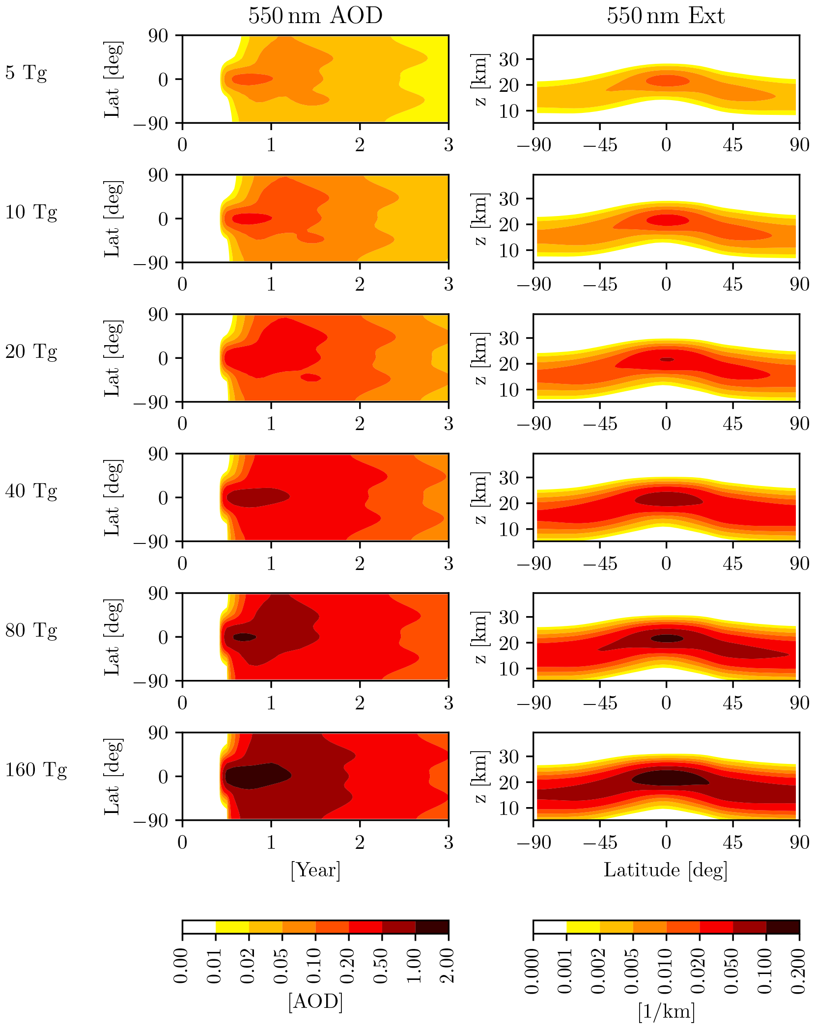
Figure 1 The EVA aerosols for eruptions used in this study. All eruptions are in June and at the Equator, with injections of 5, 10, 20, 40, 80, and 160 Tg(S), from top to bottom. Left column: zonally averaged, 550 nm aerosol optical depth (AOD) for the first 3 years of forcing. Right column: zonally averaged, latitude–height distribution of extinction coefficients (Ext), averaged over the first winter (December–January–February) following the June eruptions. Rows are labeled by the mass (in Tg) of the sulfur injection.

We recognize that, since it was calibrated on the 1991 Pinatubo eruption, EVA's accuracy for large injections is not easily validated – due to the dearth of observations and the large intermodel spread (see, e.g., Clyne et al., 2021) – and could therefore be partially unrealistic. Nonetheless, the EVA framework offers a simple, reproducible, and methodical way of exploring progressively larger eruptions. Importantly, it also allows us to compare results with those of Azoulay et al. (2021), who also used EVA forcings such as ours, and who simulated eruptions with injection amplitudes of 2.5, 5, 10, and 20 Tg(S).

2.3 The model simulations

Prior to simulating individual eruptions, we carry out a 230-year control integration with pre-industrial forcings, including pre-industrial background aerosols as defined by the EVA. We discard the first 30 years of that integration, as the model equilibrates (at least in the atmosphere) to the EVA background aerosols which are different from the historical aerosols used for the pre-industrial integrations performed for CMIP6. We then use the remaining 200 years to evaluate the unforced interannual variability, and to select initial conditions for our idealized eruptions.

Next, for each of the six injection amplitudes detailed above, we perform a set of 20 simulations, each integrated for 10 years. The 20 members of each ensemble share identical forcings, and only differ in their initial conditions. The 20 different initial conditions are chosen from the 200-year control. Specifically, to avoid confounding the response to the eruption with El Niño Southern Oscillation, the initial conditions for all eruptions are selected to be on 1 June of ENSO-neutral years, which we identify using the widely used Niño 3.4 index (Trenberth, 1997). Furthermore, all initial conditions are separated by at least a decade, to ensure sample independence.

While some studies have suggested that the winter warming signal is insensitive to the ENSO phase (e.g., Christiansen, 2008; Thomas et al., 2009), those suggestions have recently been questioned (Coupe and Robock, 2021). In keeping with our overall approach to avoid unnecessary confusion, therefore, we focus here solely on ENSO-neutral eruptions. We intend to investigate the role of different ENSO initial conditions in a subsequent study.

2.4 The post-eruption anomalies

Two ways for computing the post-eruption anomalies have been previously employed in the literature. We will be using both in this study, as appropriate. We will also show that they yield similar results. In both cases, we will focus uniquely on the December–January–February (DJF) mean in the first post-eruption winter. In fact, we will demonstrate that there is no good reason to include the second post-eruption winter as suggested in some earlier studies (e.g., Robock and Mao, 1992; Stenchikov et al., 2002).

First, the post-eruption anomalies can be defined as the paired difference from the pre-industrial (PI) control integration beginning with the same initial conditions (e.g, as in DallaSanta et al., 2019). This definition has the advantage of isolating the forced response from any concurrent low-frequency variability (i.e., anything slower than the 6-month timescale from the June eruption to the first DJF). Its disadvantage is that a companion “unperturbed” model integration – i.e., one without the volcanic eruption – is needed. Hence, such anomalies cannot be evaluated for reanalyses, or for temperature reconstructions, or for many existing model simulations (including the CMIP output). We will refer to them as the “difference-from-control-run” anomalies and designate them with the symbol Δ.

Second, the post-eruption anomalies can be defined as the difference from the average of a specified number of years prior to the eruption (typically 3 or 5 years, or more; e.g., Driscoll et al., 2012). We will refer to these as the “difference-from-reference-period” anomalies, and designate them with the symbol Δ^′. This definition, which has been widely used in the literature, has the advantage of being equally applicable to model output and to reanalyses or reconstructions; it is thus ideal for comparing model simulations to observations. While it suffers from the possible interference of low-frequency natural variability, it can be validated by varying the length of the pre-eruption reference period, to ensure that the results do not significantly depend on that length, as was done by Polvani and Camargo (2020). To be consistent with that paper, here we use the five winters prior to the June eruption as the reference period. We have checked that our conclusions are unchanged when using only three prior winters as the reference period.

2.5 The response and its significance

In this study we define the “response” of a quantity X to an eruption with a given injection amplitude as the ensemble mean of the anomalies in the first post-eruption winter, designated $\stackrel{\mathrm{‾}}{\mathrm{\Delta }X}$. Since individual members are identically forced and only differ in their initial conditions, averaging over the latter removes (to some extent, at least) the influence of internal variability, leaving behind the forced response. This method, pioneered by Deser et al. (2012), is now widely used and should not be controversial. We emphasize, however, that it is incorrect to average together eruptions with differing stratospheric injections, as that confounds forced responses of different amplitudes.

To assess the significance of the response we employ several approaches. First, we use a canonical t test (e.g., Von Storch and Zwiers, 2002, Sect. 6.6.6). Since each model run with an eruption is paired with the corresponding time period in the PI control with same initial conditions but without the eruption, for any quantity X of interest we compute ΔX, the difference between the run with the eruption and the paired period in the control run. The t statistic is then defined as $t\equiv \stackrel{\mathrm{‾}}{\mathrm{\Delta }X}\sqrt{N}/\mathit{\sigma }$, where $\stackrel{\mathrm{‾}}{\mathrm{\Delta }X}$ is the ensemble mean of ΔX, σ its standard deviation across the ensemble, and N is the size of the ensemble. This statistic is compared against tabulated values for rejection of the null hypothesis (i.e., $\stackrel{\mathrm{‾}}{\mathrm{\Delta }X}=\mathrm{0}$) at 95 % confidence with N=20 members.

An important theme of this study is the relation between $\stackrel{\mathrm{‾}}{\mathrm{\Delta }X}$, σ, and N. It is well appreciated that an arbitrarily small signal can be made statistically significant by using a sufficiently large ensemble, scaling as $N\sim (\stackrel{\mathrm{‾}}{\mathrm{\Delta }X}{)}^{-\mathrm{2}}$. Therefore, an alternative way to evaluate the importance of the response is to turn things around and ask instead: given $\stackrel{\mathrm{‾}}{\mathrm{\Delta }X}$ and σ, what is the smallest value of N for which the null hypothesis can be rejected at the 95 % level? This is accomplished by solving $t\left(N\right)/\sqrt{N}=\stackrel{\mathrm{‾}}{\mathrm{\Delta }X}/\mathit{\sigma }$ for N. The solution, denoted N_min, is obtained numerically using the values of t(N) for a 95 % confidence level. The quantity N_min offers a different perspective on the response: when N_min is very large, we deduce that the response is tiny, since a huge ensemble is needed to establish whether it is statistically significant.

Even more naively, leaving aside any consideration of ensemble size, we will consider the simple signal-to-noise ratio $\stackrel{\mathrm{‾}}{\mathrm{\Delta }X}/\mathit{\sigma }$. When this quantity is smaller than 1, the signal is smaller than the noise: this fact speaks for itself. But there is an even more important version of signal-to-noise that we also wish to consider. For any variable X of interest, in our case Eurasian winter surface temperature, primarily, we compute from the long pre-industrial control run the standard deviation of the quantity Δ^′X, i.e., the difference between X in any winter and X averaged over the preceding five winters: this quantity represents the internal – i.e., unforced – fluctuations of the variable X, and we refer to its standard deviation as σ_IV. For $\stackrel{\mathrm{‾}}{{\mathrm{\Delta }}^{\prime }X}$ computed as the ensemble mean over post-eruption winters, therefore, the signal-to-noise ratio, $\stackrel{\mathrm{‾}}{{\mathrm{\Delta }}^{\prime }X}/{\mathit{\sigma }}_{\mathrm{IV}}$, tells us whether the response to the eruption exceeds the internal variability. As we will argue below, this quantity is the one that ultimately matters when trying to determine whether the response to an eruption of specific amplitude is of practical importance.

2.6 The Northern Annular Mode

Since the proposed stratospheric pathway mechanism involves the acceleration of the stratospheric polar vortex and the accompanying poleward shift of the tropospheric mid-latitude jet due to stratospheric–troposphere coupling, it is common to characterize the extratropical circulation response as a positive phase of the Northern Annular Mode (NAM). This can be quantified from the zonal mean zonal wind following DallaSanta et al. (2019), as we do here, or from the polar-cap averaged geopotential, as described in Baldwin and Thompson (2009). Both lead to very similar results.

Our NAM computation is as follows: we define the NAM for each vertical level using monthly zonal mean zonal wind in the control run. Attention is restricted to winter (DJF) zonal wind anomalies north of 30^∘, obtained by subtracting the climatological mean. Then, the first principal component (i.e., the time series) is obtained using the first eigenvector of the latitude-weighted covariance matrix. Lastly, the principal component is regressed onto the unweighted zonal wind anomalies to obtain the spatial pattern of the NAM. The associated eigenvalue reflects the fraction of the month-to-month variance captured by the NAM. As we will show, the NAM provides a useful framework for interpreting the signal-to-noise ratio.

3 Response of the atmospheric temperature and circulation

Before discussing any Eurasian surface warming, we need to start by examining stratospheric temperature and circulation responses, to determine whether the volcanic aerosols in the lower tropical stratosphere are able to accelerate the polar vortex, with an accompanying positive phase of the NAM in the first DJF following the eruptions. The difference-from-control-run response of the atmospheric temperature T, as a function of latitude and height, for the first winter (DJF) followed each eruption is shown in the left column of Fig. 2. It is very clear that as the sulfur mass injection is increased from 5 to 160 Tg(S), the volcanic aerosols in the tropical lower stratosphere cause a progressively larger warming response, which reaches into the mid-latitudes for the larger amplitudes.

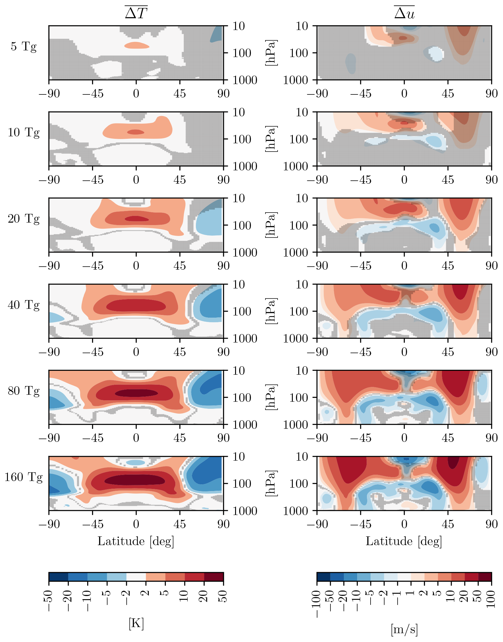
Figure 2 Zonal mean response of the atmospheric temperature ($\stackrel{\mathrm{‾}}{\mathrm{\Delta }T}$, left column) and zonal wind ($\stackrel{\mathrm{‾}}{\mathrm{\Delta }u}$, right column) in the first DJF following the June eruptions, for injections of 5, 10, 20, 40, 80, and 160 Tg(S), from top to bottom. Gray shading indicates the lack of a statistically significant response, from a t test at the 95 % confidence level.

As expected from thermal wind balance, a similar response is seen in the zonal mean zonal wind u (Fig. 2, right column), with a progressively stronger polar vortex acceleration in the NH with stronger eruptions. Note that, in these idealized calculations, 20 Tg(S) are required to obtain a statistically significant vortex acceleration. At 10 Tg(S), an amplitude comparable to that of the 1991 Pinatubo eruption, 20 members are not sufficient to establish statistical significance. However, with a larger ensemble, size significance can be established for a 10 Tg(S) eruption, as documented originally by Bittner et al. (2016). In fact, Azoulay et al. (2021) report a significant polar vortex acceleration for even smaller EVA injections, down to 5 Tg(S) in their model, using 100-member ensembles. However, the very fact than 20 eruptions are not sufficient to establish significance speaks to the fact that the signal is small for injections smaller than 10 Tg(S), even in the stratosphere.

But let us now turn to the tropospheric circulation. In the right column in Fig. 2 one can see a clear dipole in the NH tropospheric mid-latitudes, which is statistically significant for injections of 20 Tg(S) and above, in our model. This dipole, which is most prominent over the North Atlantic (not shown), represents a poleward shift in the eddy-driven jet. It is customary to quantify such jet shifts in terms of the NAM, also known as the Arctic Oscillation, which has become a standard metric for stratosphere–troposphere coupling (e.g., see Baldwin, 2000). To illustrate the NAM in our model, the zonal mean zonal winds associated with 1 standard deviation of the NAM index are shown in Fig. 3a: notice how the NAM regressed winds resemble the Δu response in Fig. 2. This suggests that the NAM is likely to be a key tool in understanding the wind response. It is also worth emphasizing that the NAM explains a large fraction of unforced variability in u, as seen in Fig. 3b: over 50 % in the troposphere and over 75 % in the stratosphere.

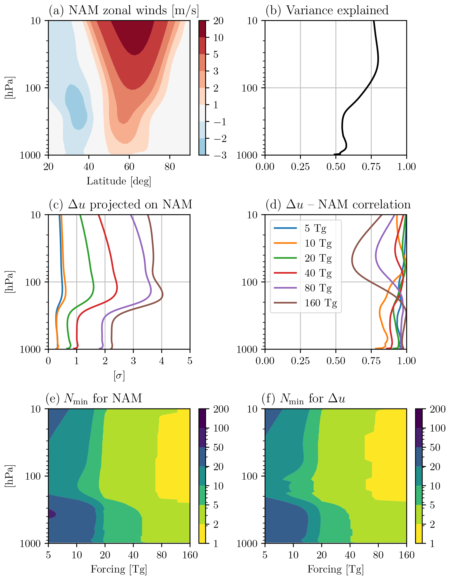
Figure 3 (a) Zonal mean zonal winds associated with 1 standard deviation of the Northern Annular Mode (NAM) in our PI control run (see Sect. 2.6 for details). (b) Fraction of variance captured by the NAM in the control run. (c) Projection of Δu (Fig. 2, right) onto the NAM, in units of the NAM standard deviation computed from the PI control run. (d) Latitude-weighted correlation of Δu and the NAM at each level. The legend in (d) also applies to (c): the colors indicate different injections. (e) Smallest ensemble size (N_min) necessary for the NAM response to be significant at the 95 % confidence level in the first-DJF NAM. (f) As in (e), but for the spatial pattern of Δu.

To express the zonal wind response to the eruptions in NAM terms, we project Δu onto the NAM index, at each level, and plot this in units of the NAM standard deviation (σ) in Fig. 3c. Notice that the tropospheric response below 250 hPa is considerably smaller than the stratospheric response: except for the two most extreme cases, the tropospheric wind response is comparable to, or smaller than, the natural variability of the NAM, i.e., the signal-to-noise ratio is less than one. If indeed the Eurasian surface temperature anomalies following the eruption are driven by the stratospheric pathway mechanism via the NAM, they are also unlikely to exceed natural variability, except possibly for the largest injections. This will be carefully analyzed and discussed in the next section.

An alternative way of quantifying the zonal wind response in the context of natural variability is to ask: how many ensemble members are required to establish statistical significance? The answer to this is illustrated in Fig. 3e and f, where the N_min values, computed as detailed in Sect. 2.5, are shown for winter post-eruption NAM and Δu, respectively. For both quantities, for injections smaller than 20 Tg(S) more than 20 eruptions are typically needed to establish a statistically significant response of the circulation in the troposphere. Thus, an individual event, such as the 1991 Pinatubo eruption, would be unremarkable in terms of its wind response: we remind the reader that, in fact, the polar vortex was anomalously weak – not strong – in winter 1991–1992, in spite of the volcanic aerosols present in the tropical lower stratosphere (see Polvani et al., 2019, and the discussion therein). Furthermore, assuming our idealized eruptions are representative of actual eruptions, even a 40 Tg(S) injection – which is more than 30 % larger than the 1815 Tambora injection – would require between 5 and 10 eruptions before a statistically significant signal in the tropospheric circulation at mid-latitudes could be ascertained. It is sobering to realize that there is only one eruption with a stratospheric sulfur injection larger than 40 Tg(S) in the past 2000 years (Samalas, in 1257), and possibly a second one if one reaches back to the past 2500 years (see Table 2 of Toohey and Sigl, 2017).

Lastly, before turning to surface temperatures, we wish to briefly discuss the response of the atmospheric circulation in the second winter after the eruption. There is some confusion on this matter in the literature: earlier studies suggested the presence of a considerable response in the second winter (e.g., Robock and Mao, 1995; Stenchikov et al., 2002; Fischer et al., 2007), whereas later studies have agreed that only the first winter should be considered (e.g., Bittner et al., 2016; Zambri and Robock, 2016; Polvani et al., 2019), since there is essentially no memory in the stratosphere to carry the response 18 months after the eruptions, when the bulk of the aerosols are no longer in the stratosphere. To provide further evidence in support of the more recent consensus, we show the time series of the NAM response in our model for 3 whole years after the eruption, at three different levels (10, 100, and 850 hPa) and for all stratospheric injections from 5 to 160 Tg(S). As one can see in Fig. 4c, at 850 hPa there is no statistically significant NAM response in the second winter after the eruption (except, possibly, for the very largest injection mass) and thus no reason to expect a response in Eurasian surface temperatures, to which we now turn our attention.

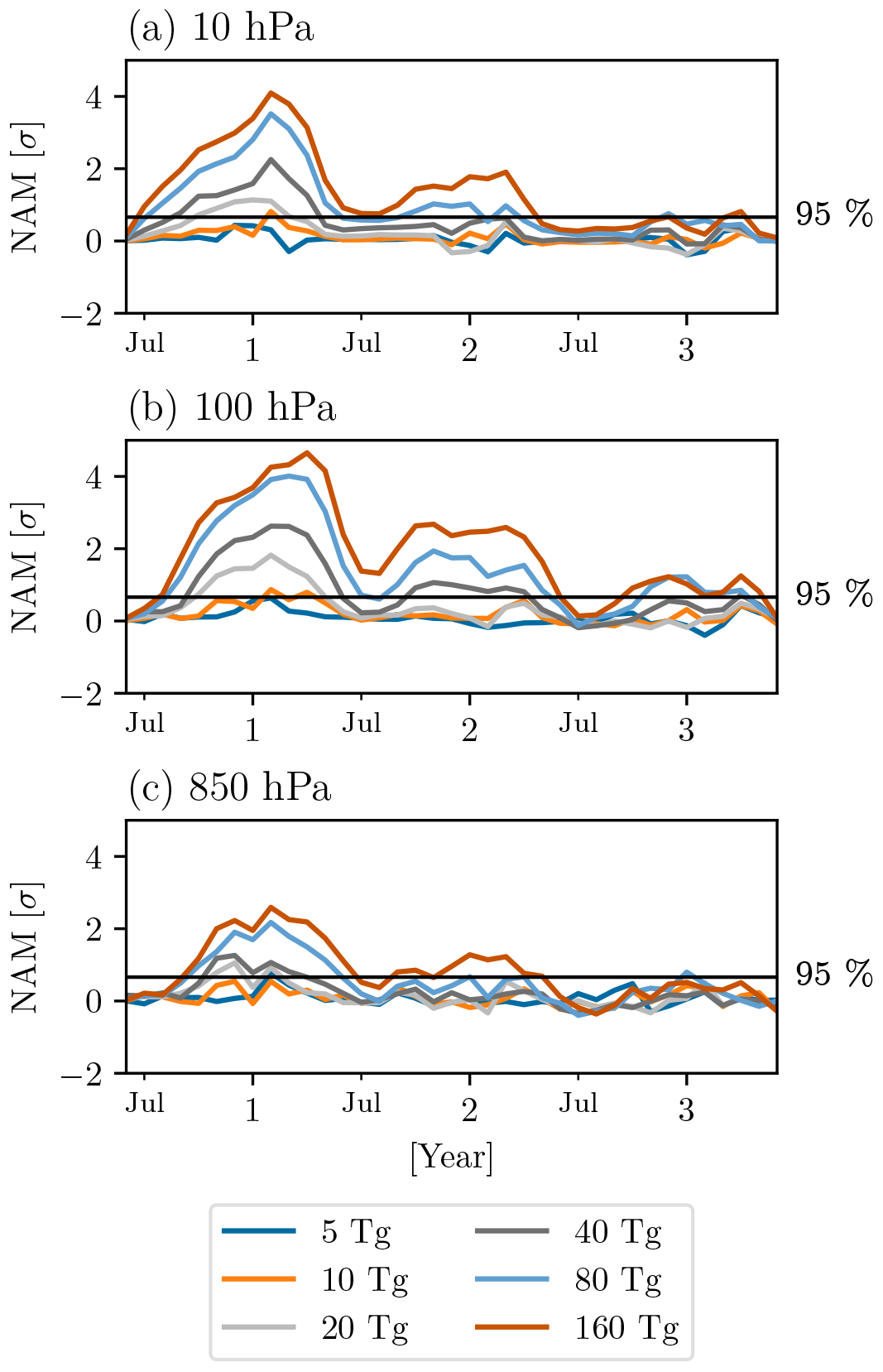
Figure 4 Monthly evolution of the NAM response for 3 years after the June eruptions, with the 95 % confidence significance level indicated by the black horizontal line, at (a) 10 hPa, (b) 100 hPa, and (c) 850 hPa. The units on the ordinate are standard deviations of the NAM from the PI control (σ). On the abscissa, the numbers 1, 2, and 3 designate the first, second, and third January after the eruption.

4 Response of the winter surface temperature over Eurasia

The starting point of this discussion is the quantity ΔT_s, the surface temperature anomaly, computed using the difference-from-control-run method, in the first post-eruption winter. Its ensemble mean $\stackrel{\mathrm{‾}}{\mathrm{\Delta }{T}_{\mathrm{s}}}$ , shown in the left column of Fig. 5, represents the forced response caused by the eruption for each injection amplitude. It is readily seen that for our idealized EVA eruptions, a statistically significant warming response starts to emerge for 20 Tg(S) injections over parts of eastern Eurasia, and covers most of Eurasia for 40 Tg(S) and above. To quantify this more carefully over Eurasia, we start by considering the region 40–70^∘ N and 0–150^∘ E, for consistency¹ with previous studies (Polvani et al., 2019; Polvani and Camargo, 2020; Azoulay et al., 2021). As seen in Table 1, the forced response $\stackrel{\mathrm{‾}}{\mathrm{\Delta }{T}_{\mathrm{s}}}$ becomes statistically significant over that region only with an 80 Tg(S) injection. However, a careful inspection of the red areas in the left column of Fig. 5 suggests that 40–70^∘ N might not be the best choice of latitudes if one is trying to capture the largest Eurasian warming.

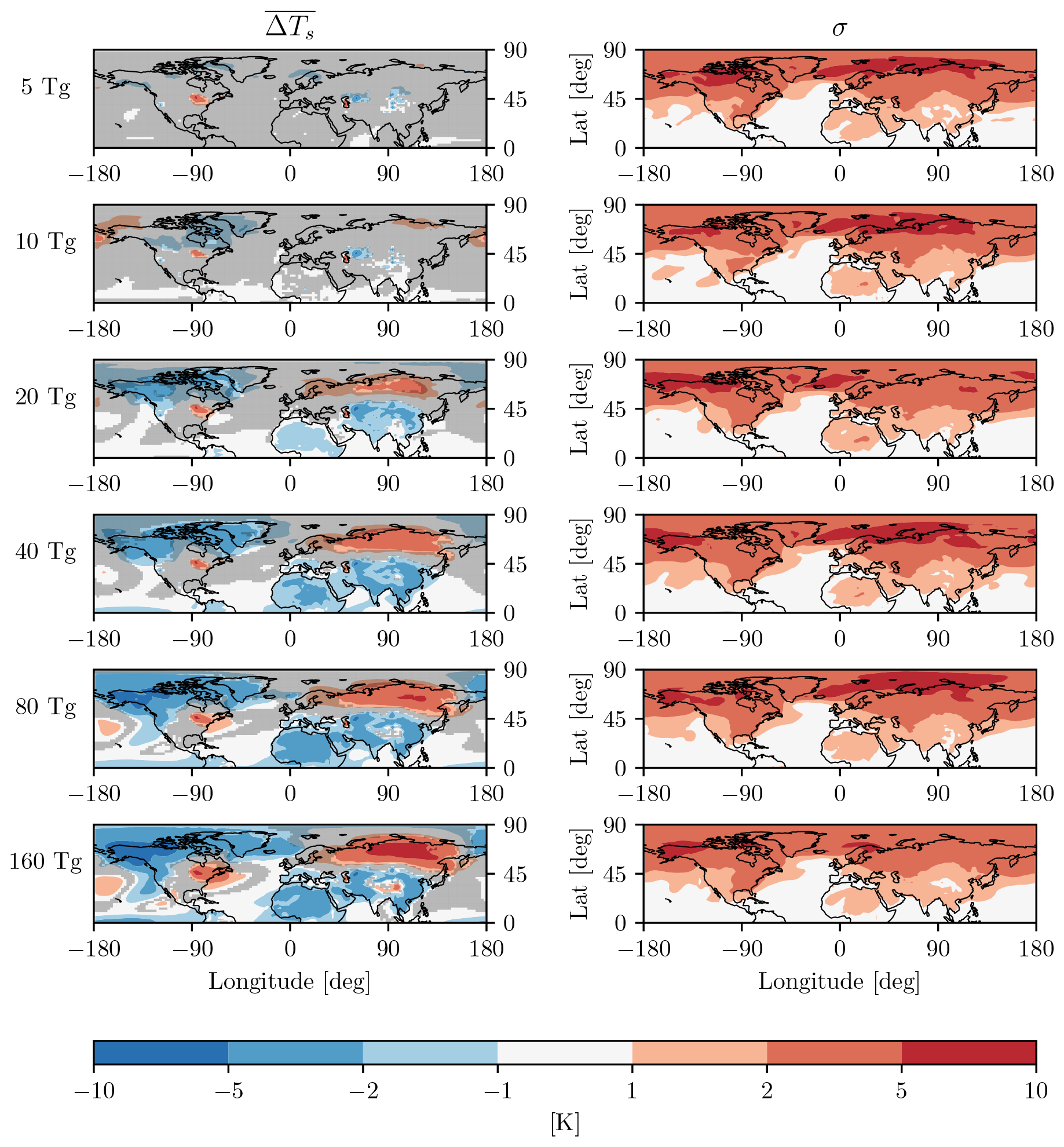
Figure 5 The surface temperature response ΔT_s (left) and the corresponding ensemble standard deviation σ (right) for the first winter (DJF) following the eruptions. Rows show increasing injection amplitudes, from 5 to 160 Tg(S), top to bottom, as labeled. Gray shading indicates the lack of a statistically significant response at the 95 % confidence level using a t test.

Table 1 Statistics of surface temperature anomalies, averaged over Eurasia, in the first post-eruption winter (DJF) following idealized low-latitude eruptions with injections from 5 to 160 Tg(S). Two averaging regions are considered: 40–70^∘ N, 0–150^∘ E (as in Polvani et al., 2019; Polvani and Camargo, 2020) and 50–80^∘ N, 0–150^∘ E (as in Azoulay et al., 2021). For each averaging region, $\stackrel{\mathrm{‾}}{\mathrm{\Delta }{T}_{\mathrm{s}}}$ is the ensemble mean anomaly (the response) computed using the difference-from-control-run method, σ the corresponding standard deviation, and N_min the minimum ensemble size needed to obtain a response that is statistically significant at the 95 % confidence level. Injection amplitudes for which N_min>20 produce responses that are not statistically significant at that level with 20-member ensembles; these insignificant responses are followed by an asterisk. $\stackrel{\mathrm{‾}}{{\mathrm{\Delta }}^{\prime }{T}_{\mathrm{s}}}$ is the response computed using the difference-from-reference-period method.

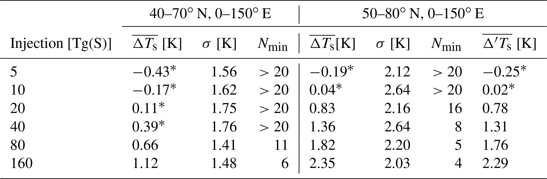
Therefore, following the suggestion in Azoulay et al. (2021), we will focus on the more northerly region 50–80^∘ N over the same longitude range 0–150^∘ E, in order to maximize the volcanically forced surface warming. We will refer to this as the “standard” Eurasian region. As seen in Table 1, over that region the response becomes significant with only a 20 Tg(S) injection. In fact, Azoulay et al. (2021) report that the response is significant even for a 10 Tg(S) injection over that region. This is not at odds with our results, considering our smaller 20-member ensembles compared with their 100-member ensembles. Although N_min computed as per the method of Sect. 2.5 cannot be directly evaluated for small injections owing to the tiny value of $\stackrel{\mathrm{‾}}{\mathrm{\Delta }{T}_{\mathrm{s}}}$, which results in a near division by zero, we can estimate it via extrapolation as follows: assuming the response to be approximately linear for the small injections, and noting that $N_{\min }\propto (\mathrm{1}/{\stackrel{\mathrm{‾}}{\mathrm{\Delta }{T}_{\mathrm{s}}}}^{\mathrm{2}})\propto (\mathrm{1}/A^{\mathrm{2}})$, where A is the injection amplitude, a halving of the injection would require a 4-fold increase in N_min. Since N_min=16 for 20 Tg(S) in our model, we deduce a value of N_min=64 for 10 Tg(S) and N_min=256 for 5 Tg(S). These numbers are perfectly in line and thus confirm the findings of Azoulay et al. (2021) who, with 100-member ensembles, found a significant warming for 10 Tg(S) but not for 5 Tg(S) injections.

Since a 10 Tg(S) injection is quite close to the one accompanying the 1991 Pinatubo and the 1883 Krakatau eruptions (each close to 9 Tg(S); see Toohey and Sigl, 2017), one wonders why recent modeling studies have found no statistically significant winter warming following those eruptions (Bittner, 2015; Polvani et al., 2019; Polvani and Camargo, 2020; Azoulay et al., 2021). The answer rests in the fact that the EVA aerosols are sufficiently different from the ones used in the standard CMIP5 and CMIP6 historical simulations to generate a stronger response which, given a large enough ensemble, can yield statistical significance for a 10 Tg(S) injection. We discuss this more in Appendix A and also refer the reader to Azoulay et al. (2021) who also show that, even with a 100-member ensemble, non-idealized aerosols yield no significant post-Pinatubo warming response in their model.

But let us focus on injections larger than Pinatubo and Krakatau, for which our model does show a statistically significant Eurasian warming response. For the standard Eurasian region, our model simulates a post-eruption winter warming of 0.83 ^∘C for a 20 Tg(S) injection, and this warming grows monotonically up to 2.35 ^∘C at 160 Tg(S), as seen in Table 1. While these values may appear considerable, we now argue that they are small in the context of internal variability. There are several ways to show this.

First, we draw the reader's attention to the magnitude of the ensemble spread, as quantified by the standard deviation σ. This quantity is shown in the right column of Fig. 5, and we emphasize that the colorbar for σ is identical to the one for $\stackrel{\mathrm{‾}}{\mathrm{\Delta }{T}_{\mathrm{s}}}$. Notice that over most of Eurasia, $\stackrel{\mathrm{‾}}{\mathrm{\Delta }{T}_{\mathrm{s}}}<\mathit{\sigma }$ for both 20 and 40 Tg(S) injections. In fact, averaging over our standard Eurasian box, we see that the signal-to-noise ratio $\stackrel{\mathrm{‾}}{\mathrm{\Delta }{T}_{\mathrm{s}}}/\mathit{\sigma }<\mathrm{1}$ even for 80 Tg(S); and, even for the very largest injection amplitude, 160 Tg(S), the Eurasian signal-to-noise ratio is a meager 1.16 – a rather unimpressive value if one considers that a 160 Tg(S) injection is almost three times the size of the the largest known volcanic injection of the past 2500 years (Samalas, in 1257, with a 59 Tg(S) injection, as estimated by Toohey and Sigl, 2017).

Second, to further appreciate how small the post-volcanic surface temperature response is in the context of internal variability, we present in Fig. 6 the warmest (right column) and coldest (left column) simulation found in each 20-member ensemble, for all injection amplitudes. Remarkably, even for a massive 160 Tg(S) injection, one can find an event with temperatures that are anomalously cold over Eurasia in the first winter after the eruption. In addition, we note that this can be captured with our relatively small 20-member ensemble.

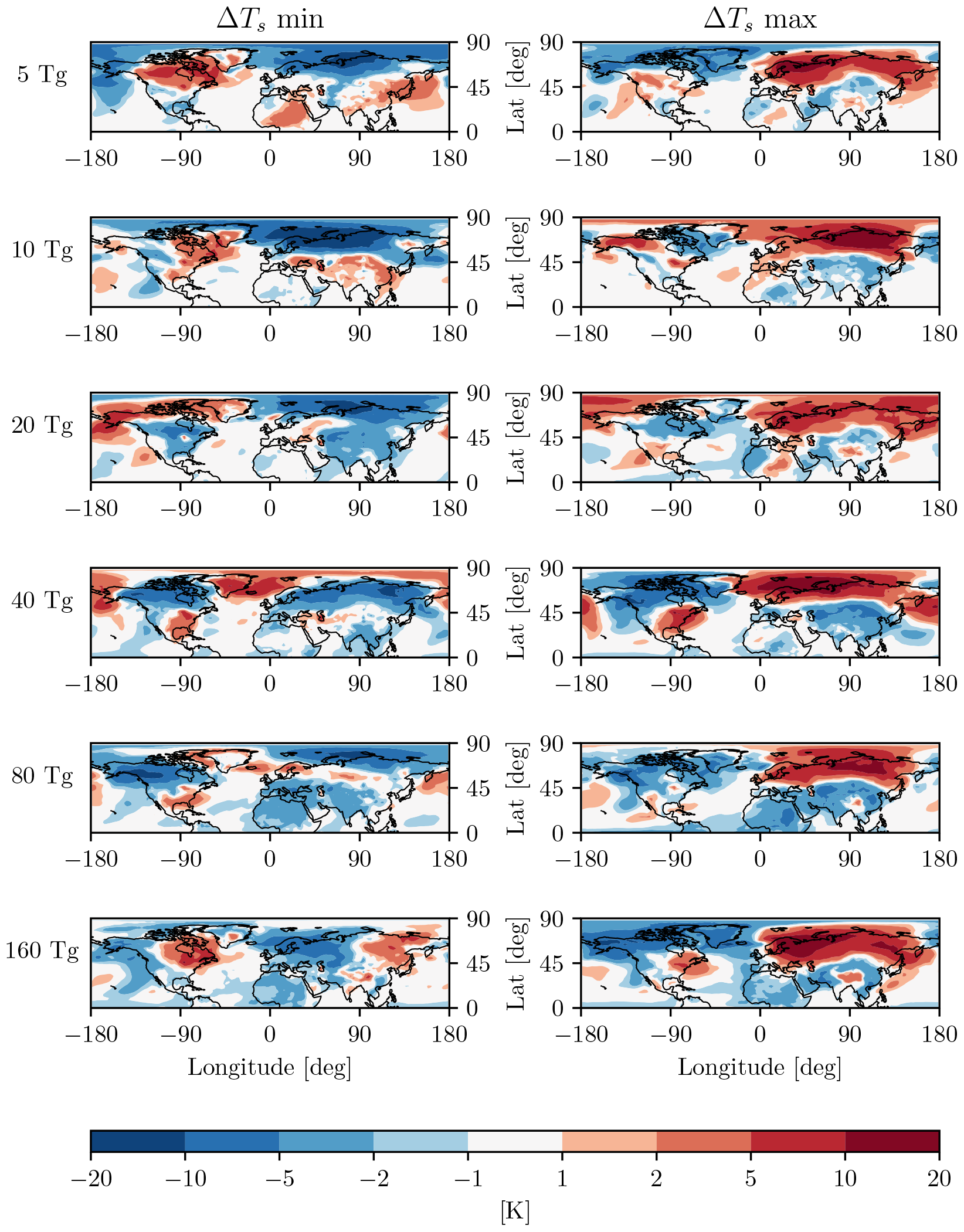
Figure 6 Coldest (left) and warmest (right) winter surface temperature anomalies over Eurasia in each 20-member ensemble, from 5 to 160 Tg(S), top to bottom, as labeled. Note that the colorbar covers twice the range as the one in Fig. 5, as the variability is larger than the response, even for very large sulfur injections.

Third, and most importantly, we now quantitatively compare the forced post-eruption winter warming to the unforced interannual variability, as done in Polvani and Camargo (2020). To do this, we start by computing the response $\stackrel{\mathrm{‾}}{{\mathrm{\Delta }}^{\prime }{T}_{\mathrm{s}}}$, where anomalies are computed using the five pre-eruption winters as the reference period (see Sect. 2.4). As one can see from Table 1, this quantity is very similar to the difference-from-control-run response $\stackrel{\mathrm{‾}}{\mathrm{\Delta }{T}_{\mathrm{s}}}$, over the entire range of amplitudes. This confirms that our findings are robust. For the sake of completeness, box-and-whisker plots of $\stackrel{\mathrm{‾}}{{\mathrm{\Delta }}^{\prime }{T}_{\mathrm{s}}}$ averaged over several different Eurasian regions are shown in Fig. 7, where the EVA response can be directly compared to one from Pinatubo and Krakatau. The green bars, for the region used in Polvani et al. (2019), indicate that an 80 Tg(S) injection is needed for significance. But using the more northerly standard region, shown in the light blue bars, we see that 20 Tg(S) suffices to capture a statistically significant warming, in agreement with the threshold value for $\stackrel{\mathrm{‾}}{\mathrm{\Delta }{T}_{\mathrm{s}}}$.

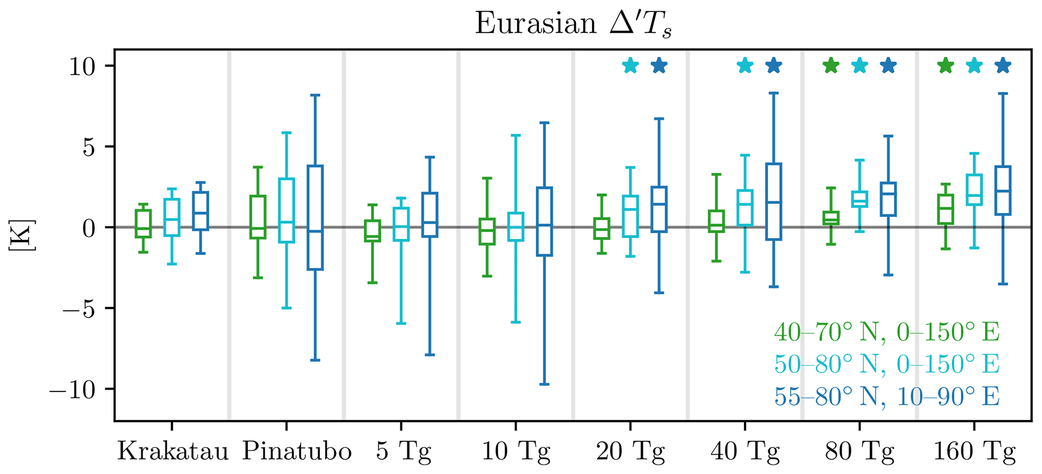
Figure 7 Eurasian surface temperature anomalies, computed using the difference-from-reference-period method, for the first winter following the indicated eruptions for both, two historical simulations and for the EVA. Colors indicate different averaging regions over Eurasia, as shown in the legend. Boxes show the upper and lower quartiles, central bars the median, and whiskers the ensemble maximum and minimum. Stars denote statistically significant responses at the 95 % confidence level.

Next, in order to contrast these $\stackrel{\mathrm{‾}}{{\mathrm{\Delta }}^{\prime }{T}_{\mathrm{s}}}$ responses to interannual variability, we compute the probability distribution function (PDF) of Δ^′T_s in the pre-industrial control run of our model, where no volcanic eruptions occur. This quantity represents the surface temperature anomalies over the standard Eurasian region originating solely from internal variability: it has a mean value of zero and, fitting a standard Gaussian to it, a standard deviation σ_IV of 1.78 ^∘C. Finally, we superimpose onto this PDF the 20 simulated eruptions for each injection amplitude, together with the ensemble mean representing the forced response.

From those plots, seen in the left column of Fig. 8, it is clear that nearly all individual post-eruption anomalies in our study fall well within the PDF of unforced anomalies. In fact, the forced response (i.e., the ensemble mean) only exceeds the interannual variability σ_IV with a 160 Tg(S) injection; and, even in that case, the forced response is only slightly larger than σ_IV, and nowhere close to 2σ_IV. This means that, even with a massive 160 Tg(S) volcanic injection, post-eruption anomalies in winter over Eurasia would be largely indistinguishable from the large anomalies that occur even in the absence of an eruption, as a consequence of the large internal variability of surface temperature at mid-latitudes.

​​​​​​​

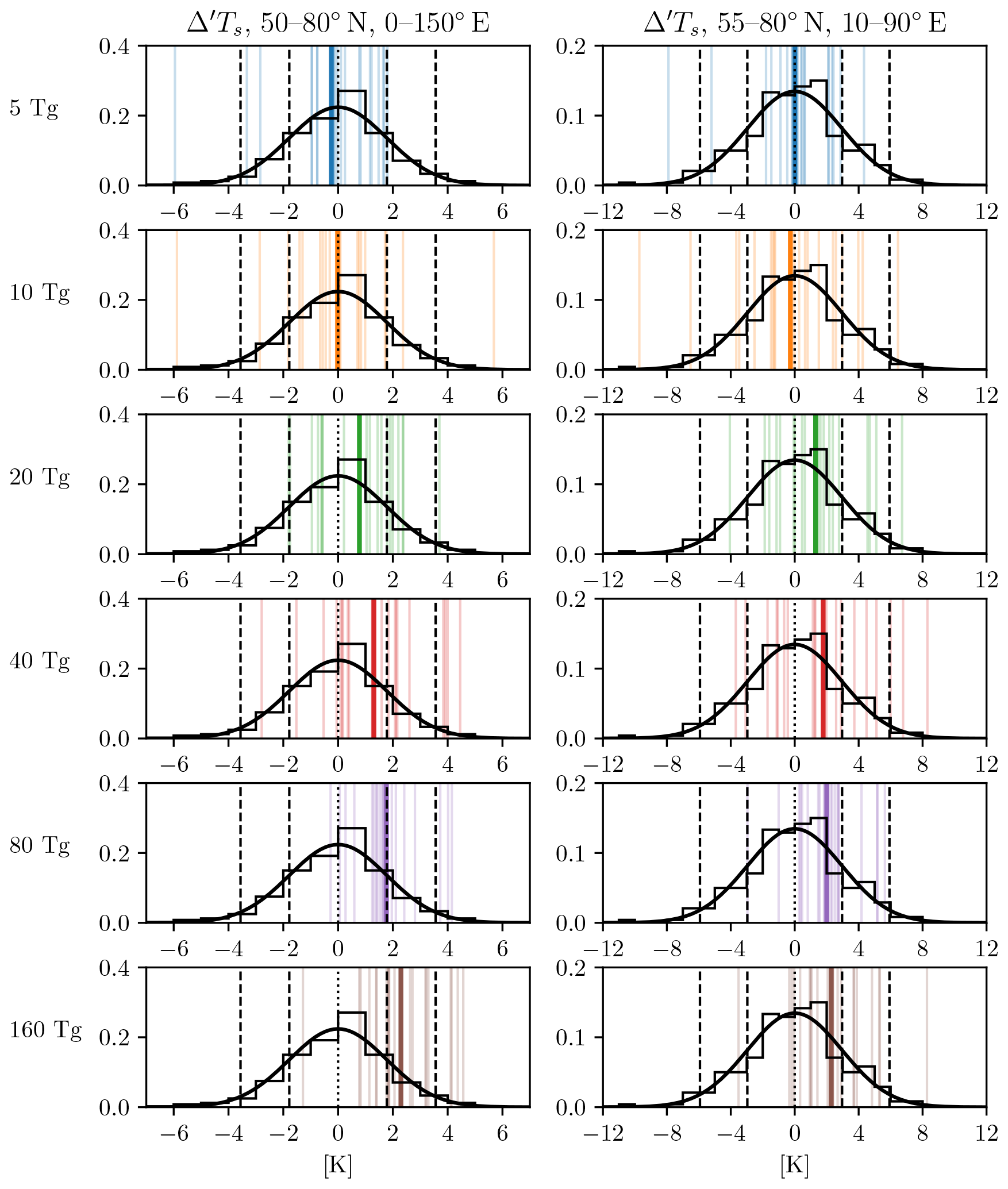
Figure 8 Eurasian winter surface temperature anomalies (computed with the difference-from-reference-period method), for each eruption (thin colored bars) and for the ensemble mean (thick colored bar), from 5 to 160 Tg(S), top to bottom, as labeled. In each panel, these are superimposed on the climatology (black) of the same quantity from the pre-industrial control runs, quantified by a histogram and a Gaussian fit, and with dashed lines indicating the 1σ and 2σ ranges, as in Polvani and Camargo (2020). Left column: average temperature over the region 50–80^∘ N and 0–150^∘ E. Right column: average temperature over the region 55–80^∘ N and 10–90^∘ E.​​​​​​​

As a final check on the robustness of our conclusion, we have explored the narrower region 55–80^∘ N and 10–90^∘ E reported by Azoulay et al. (2021) as the locus of the largest post-eruption warming over Eurasia in their model. First, in our model we find that the forced response over that region is not different from the one over the standard region, as seen in Fig. 7 (contrast the light and dark blue bars). Second, and more crucially: making the region narrower dramatically increases the interannual variability σ_IV, which goes from 1.78 to 2.96. This is seen in the right column of Fig. 8, where the axis on the abscissa needs to be expanded by a factor of two to encompass the entire PDF of unforced post-eruption surface temperature anomalies. In fact, for this narrower region the forced response is smaller than the interannual variability even for 160 Tg(S)​​​​​​​ injections. This further corroborates our conclusion.

5 Summary, discussion, and outlook

In a nutshell, we have explored the winter response to progressively larger, low-latitude eruptions using a stratosphere-resolving climate model with idealized prescribed volcanic aerosols, and two key results have emerged from our exploration. First, we have confirmed that with a sufficiently large stratospheric injection and with a sufficiently large ensemble size, statistically significant surface warming over Eurasia in the first post-eruption winter can be seen in a climate model, as reported in Azoulay et al. (2021). Second, and most importantly, we have shown that for injections up to 160 Tg(S), the first post-eruption Eurasian winter warming forced by the volcanic aerosols is sufficiently small as to be indistinguishable from internal variability. With these key findings in mind, we are now ready to address several important issues, and also to place our results in the context of earlier studies and of the observational record.

First, regarding the emergence of a statistically significant post-eruption Eurasian winter warming: the threshold for this – for the idealized EVA aerosols – is 20 Tg(S) in our model, using 20-member ensembles. Azoulay et al. (2021) report the threshold to be at 10 Tg(S) using 100-member ensembles, for the same EVA aerosols. The difference largely resides in the fact that our ensemble size is considerably smaller but, in part, may also be due to model differences. From our model, we estimate that over 64 eruptions are needed for a 10 Tg(S) injection to produce significant warming. While Azoulay et al. (2021) do not report the values of N_min, the mere fact that more than 60 events are needed speaks to how small the forced volcanic warming signal actually is in these models.

In fact, over the past 2500 years, there are only 33 eruptions with stratospheric injections estimated to be in excess of 10 Tg(S), according to the latest compilation by Toohey and Sigl (2019). Thus, assuming that EVA aerosols are representative of typical eruptions (which may not be the case; see below), and assuming that current-generation models are not lacking in significant aspects relevant to this problem, it is currently impossible to observationally validate this modeling evidence of a weak post-eruption winter warming over Eurasia given the limited eruption record. Focusing on larger eruptions would improve the signal-to-noise ratio, but that effort is similarly futile: for a 40 Tg(S) injection, our model suggests that eight events are needed to establish statistical significance, but only two such events are known to have occurred in the past 2500 years. One could look further back in time, but temperature reconstructions become even more problematic given that we are seeking a winter signal, and most tree-ring-based reconstructions are based largely on summer data (when trees actually grow).

Second, it must be kept in mind that the results in Table 1 apply only to the EVA aerosols, and some evidence suggests that these idealized aerosols at 10 Tg(S) produce more warming than the aerosols used for Pinatubo in the CMIP5 and CMIP6 model runs. For instance, Azoulay et al. (2021) found no statistically significant warming – even with 100 members – for Pinatubo when forced with an earlier aerosol reconstruction (Stenchikov et al., 1998), although their model shows significant warming with EVA aerosols at 10 Tg(S). Polvani et al. (2019) found no significant warming for Pinatubo with a 50-member ensemble of the CanESM2 model forced with CMIP5 volcanic aerosols, and Polvani and Camargo (2020) found no surface warming for Krakatau with the 100-member Grand Ensemble (Maher et al., 2019). Also, Figs. 3 and 7 of Toohey et al. (2016) indicate that the optical depth of EVA aerosols for a 9 Tg(S) injection is considerably larger than the one produced for Pinatubo by the Chemistry-Climate Model Initiative (CCMI; Eyring et al., 2013), which formed the basis for the CMIP6 forcing. It is possible, therefore, that the EVA aerosol forcing might be unrealistically large and thus overly favorable to cause Eurasian winter warming, further underscoring our key conclusion.

Third, the reader may wonder if and how our findings might be altered if the eruptions coincided with El Niño or La Niña events. The extant literature is confounding: one study has claimed that El Niño is necessary to produce winter warming over Eurasia (Coupe and Robock, 2021), but two earlier studies have reported that the winter warming signal is insensitive to the ENSO phase (Christiansen, 2008; Thomas et al., 2009). Similarly, while some modeling studies have claimed that volcanic eruptions cause El Niño (e.g., Khodri et al., 2017), others have argued that there is little evidence to support that claim (e.g., Dee et al., 2020; note: one of the referees of this paper insisted that we also cite his own critical views of that study, which can be found in Robock, 2020). The very existence of such contradictory claims in the peer-reviewed literature is a strong indication of a very small signal, at best. In fact, preliminary results from our model show no significant ENSO impacts on winter warming in the Northern Hemisphere, and we plan to report on that in a future paper.

Fourth, we wish to emphasize that modeled winter surface warming reported here, and in Azoulay et al. (2021), does not validate the early modeling studies that claimed a forced winter warming following the Pinatubo eruption, but actually demonstrates how that warming was spuriously generated by those studies' inadequacies. Just to cite one example: Shindell et al. (2004), with an early GISS ModelE version at 4^∘ × 5^∘ horizontal resolution and with a mere 20 vertical levels, running with prescribed SST, reported a statistically significant winter warming over Eurasia after Pinatubo with a 5-member ensemble. This contrasts with the model used here, with over 100 vertical levels and finer horizontal resolution, which shows no forced Eurasian winter warming from Pinatubo aerosols, nor from the stronger EVA aerosols with 10 Tg(S) injection with a much larger ensemble. One might rebut that 10 years from now we will have even better models and that the conclusions reached here may again be revised. We agree that such a possibility is very real.

In fact, there is little doubt that, beyond model resolution, several aspects of our simulations are ready for improvement. Perhaps the most unrealistic aspect of the modeling setup employed here – which is common to nearly every study on the question of Eurasian post-eruption winter warming – is the fact that our volcanic aerosols are prescribed from an external file and thus inconsistent with the atmospheric circulation and composition. However, we note the existence of major uncertainties in interactive aerosol modeling, which the VolMIP community has labeled “drastic” (Clyne et al., 2021). Also, whether the dependency of the aerosol optical depth on injection mass as parameterized in the EVA is truly representative of large eruptions remains an unanswered question, owing to the lack of observations. In any event, what emerges from our study, which independently confirms the findings of Azoulay et al. (2021), is that the early claims of robust Eurasian winter warming for eruptions such as Pinatubo – and even smaller ones, such as the 1982 El Chichón or the 1962 Agung eruptions – simply cannot be reproduced with current-generation climate models: they have consistently failed to show any warming for such historical eruptions, because the signal-to-noise ratio is simply too small.

Fifth, and most importantly, our simulations clearly demonstrate that the signal-to-noise ratio is not only small for eruptions with sulfur injections comparable to those of Pinatubo and Krakatau, roughly 10 Tg(S): the signal-to-noise ratio remains small all the way up to 160 Tg(S). Even with that gigantic forcing, we have found that only 3 out of 20 members produce winter warming anomalies that exceed the 2σ range of the unforced variability in the control run (see the bottom left panel of Fig. 8). In addition, if one nonetheless wanted to establish a statistically significant warming signal over Eurasia for 160 Tg(S) eruptions, at least four such events would be needed (see Table 1). Yet, not a single such eruption has occurred in the past 2500 years (Toohey and Sigl, 2017).

An alternative way to appreciate how the post-eruption response is overwhelmed by the internal variability is the following: let us look again at the 80 Tg(S) case, which is considerably larger than the 1257 Samalas eruption, the largest of the past 2500 years. For such an eruption $\stackrel{\mathrm{‾}}{\mathrm{\Delta }{T}_{\mathrm{s}}}\mathrm{}\mathrm{}\mathrm{}\mathrm{}\mathrm{}\mathrm{}\mathrm{}\sim \mathrm{1.8}$ ^∘C over Eurasia (see Table 1), and this is very close to 1 standard deviation of the interannual variability, as seen in Fig. 8 (left column, second to last panel). So, using the 68–95–99.7​​​​​​​ rule for a standard Gaussian, we deduce that 16 % of the time, the winter anomalies in the absence of an eruption, are larger than the mean anomaly following an 80 Tg(S) eruption in our model. This means that over a period of 2500 years we expect 400 winters with an anomalous warming larger than the mean post-eruption warming. This is what we mean when we say that the post-eruption warming – even for eruptions larger than any of the ones known to have occurred over the last 2500 years – would be unremarkable and indistinguishable from internal variability.

Finally, we remind the reader that the new evidence we have presented here for the possible existence of post-eruption Eurasian winter warming comes from climate models. The observational evidence, at this point, is what is clearly lacking, especially when one considers that the models are telling us that many events are needed to separate the forced response from internal variability. As already noted, most of the early observational studies reached unsubstantiated conclusions, and the evidence for a winter warming provided by the most recent, and most comprehensive, observational study (Fischer et al., 2007) is also questionable. First, only 15 eruptions were examined in that study, of which only a handful are larger than Pinatubo or Krakatau. Second, their conclusions were reached by averaging together large and small eruptions, which confounds signal and noise. Third, and most importantly, the largest warming signal was found to occur in the second post-eruption winter, a fact that we find difficult to believe given the evidence presented above (see Fig. 4). Fourth, that study was conducted with a single temperature reconstruction (Luterbacher et al., 2004) and, to date, it has not been independently confirmed with a different reconstruction. Since the models are now in good agreement in showing that the Eurasian warming signal – if it exists at all – is very small at best, more work is needed on the observational side to provide at least some plausible evidence (if not a statistically convincing demonstration) that the post-eruption winter surface warming is not a mere modeling artifact.

Appendix A: Contrasting the idealized EVA eruptions with Pinatubo and Krakatau

To evaluate the realism of eruptions simulated with the idealized EVA aerosols, we compare them with the two largest low-latitude eruptions found in the “historical” runs that were performed with our same model configuration as part of the CMIP6 (Miller et al., 2021): the 1991 Pinatubo and the 1883 Krakatau eruptions. Both of these eruptions are estimated to have resulted in approximately 9 Tg(S) injections, so we contrast them with the 10 Tg(S) case. It is important to keep in mind that the historical integrations, of which a small ensemble of six were performed independently from this study and submitted to CMIP6, also include all other climate forcings over the period 1850–2016, not simply the volcanic aerosols.

First, as shown in Fig. A1, the EVA aerosols show some clear differences to the ones prescribed by CMIP6 for Pinatubo and Krakatau, which were built as historical reconstructions. Second, in Fig. A2 we show the atmospheric wind and temperature response, computed with the difference-from-reference-period method. One can see that the tropical temperature anomalies are much broader in the meridional direction for Pinatubo and Krakatau than for the EVA, owing to a more global spread of aerosols in the CMIP6 prescription than in the EVA. This results in a weakened meridional temperature gradient and thus a weaker vortex acceleration compared with the EVA at 10 Tg(S), although the significance is very weak, even in the stratosphere, for all these eruptions, and it is actually non-existent in the troposphere. In any case, the impression here is that the EVA aerosols appear more favorable to stratospheric vortex acceleration due to their stronger meridional temperature gradient.

Third, at the surface, none of these aerosol forcings cause a statistically significant response, as shown in Fig. A3. If anything, the historical forcings seem to produce a little surface warming, although it is more centered over the pole than Eurasia and thus unlikely to be tied to the NAM. In any case, nothing here is significant, so there is little to discuss. One could argue that our ensemble sizes of 6 are too small, but Azoulay et al. (2021) show that in their model too, with a much larger 100-member ensemble, the historical Pinatubo aerosols produce no statistically significant Eurasian winter surface warming, and the same was shown for Krakatau by Polvani and Camargo (2020), also with a 100-member ensemble.

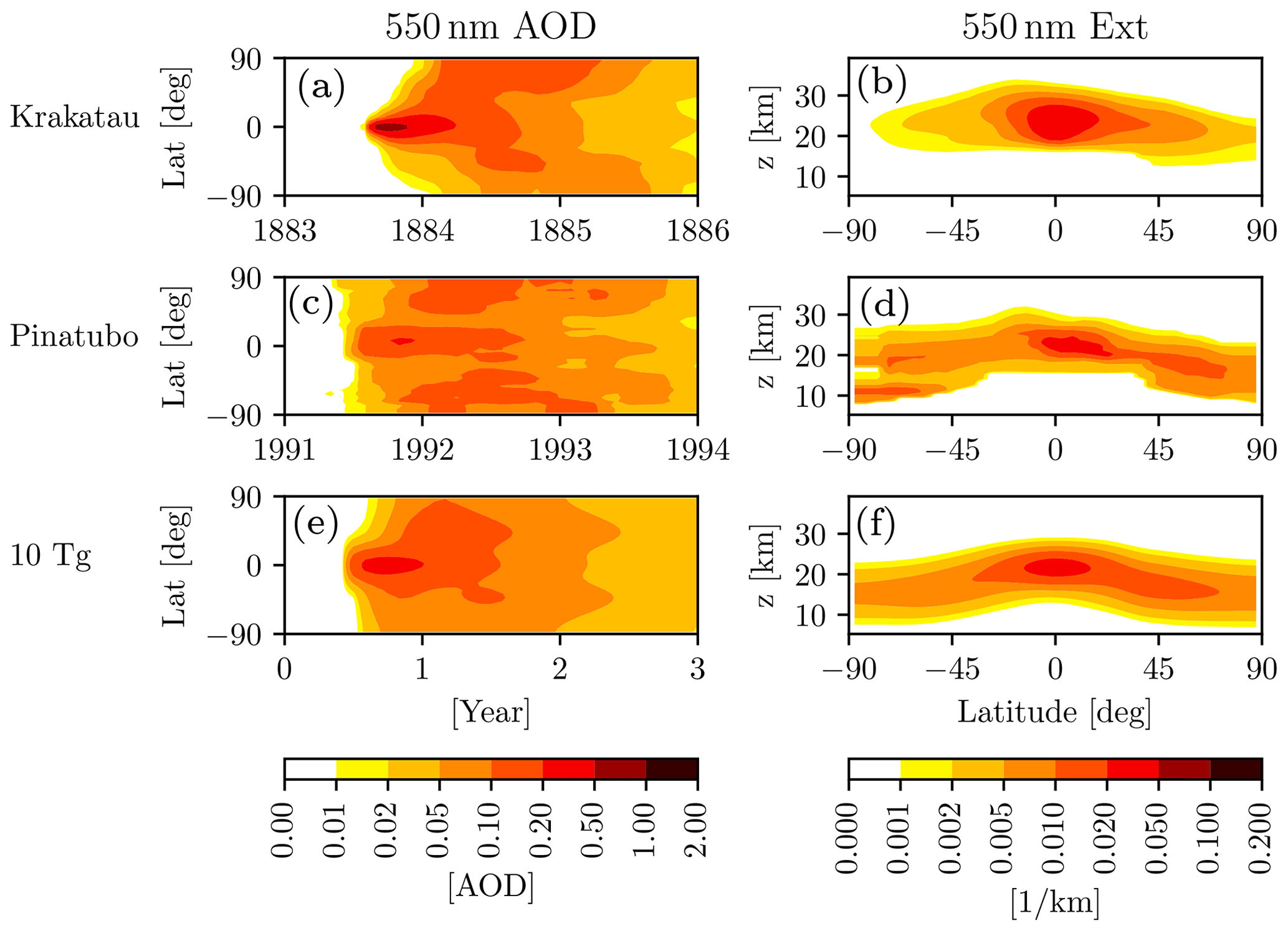
Figure A1 As in Fig. 1, but for the CMIP6 volcanic aerosol prescription (Miller et al., 2021), for Pinatubo (a, b) and Krakatau (c, d). For comparison, the EVA 10 Tg(S) aerosols are shown in (e) and (f).

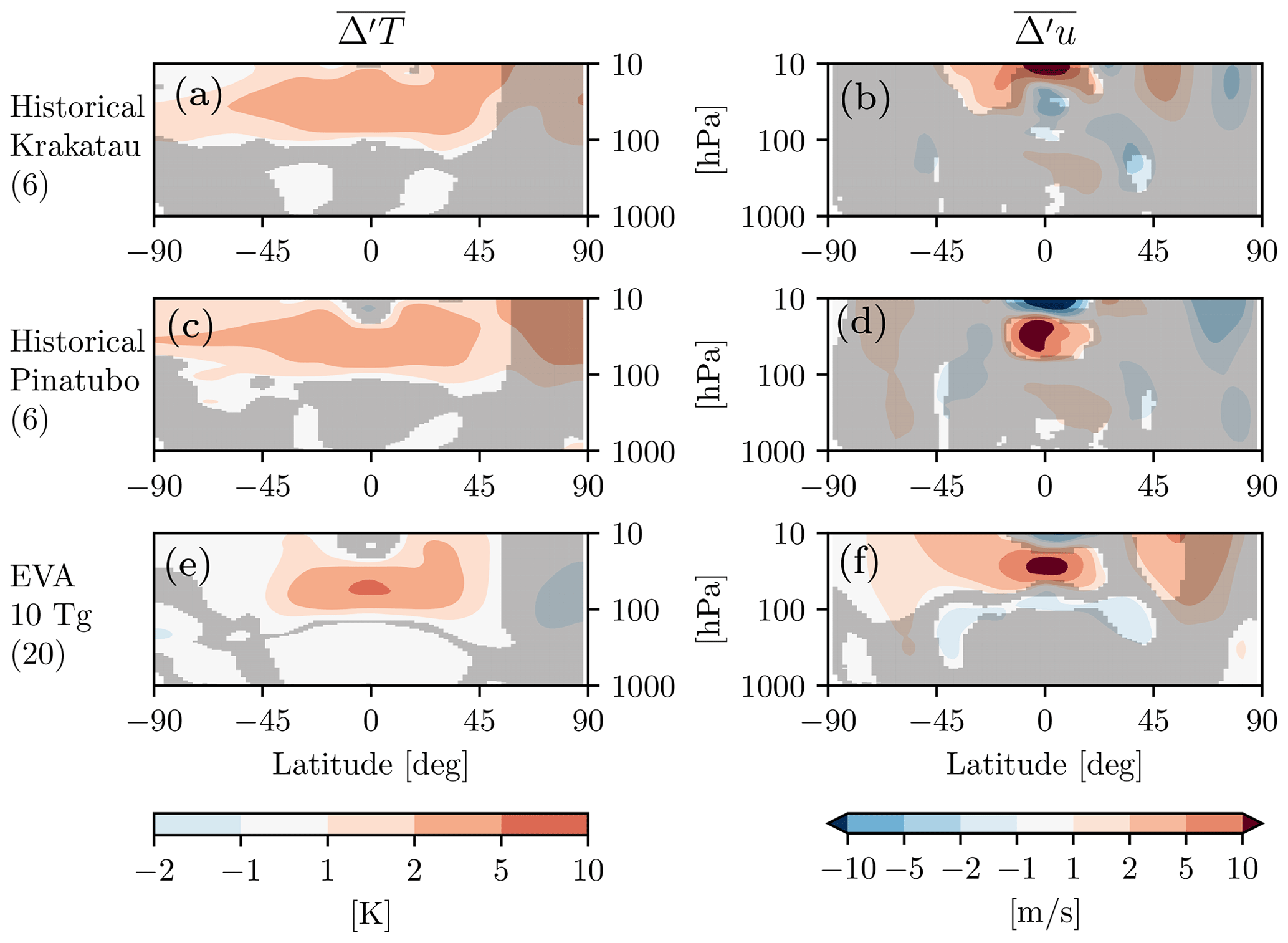
Figure A2 As in Fig. 2, but using the difference-from-reference-period method, for Krakatau (a, b), Pinatubo (c, d), and EVA aerosols at 10 Tg(S) (e, f), with the ensemble size in parentheses in (a), (c), and (e)​​​​​​​.

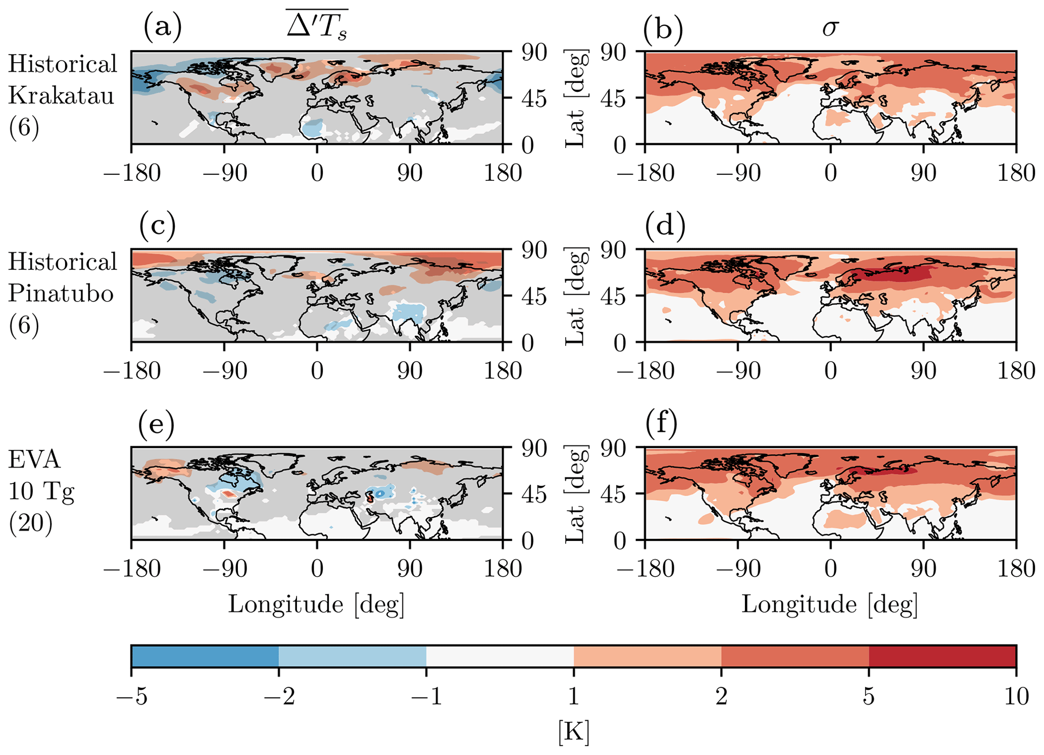
Figure A3 As in Fig. 5, but using the difference-from-reference-period method, for Krakatau (a, b), Pinatubo (c, d), and EVA aerosols at 10 Tg(S) (e, f), with the ensemble size in parentheses in (a), (c), and (e).