Improving NO_x emission estimates in Beijing using network observations and a perturbed emissions ensemble

Emissions inventories are crucial inputs to air quality simulations and represent a major source of uncertainty. Various methods have been adopted to optimise emissions inventories, yet in most cases the methods were only applied to total anthropogenic emissions. We have developed a new approach that updates a priori emission estimates by source sector, which are particularly relevant for policy interventions. At its core is a perturbed emissions ensemble (PEE), constructed by perturbing parameters in an a priori emissions inventory within their respective uncertainty ranges. This PEE is then input to an air quality model to generate an ensemble of forward simulations. By comparing the simulation outputs with observations from a dense network, the initial uncertainty ranges are constrained, and a posteriori emission estimates are derived. Using this approach, we were able to derive the transport sector NO_x emissions for a study area centred around Beijing in 2016 based on a priori emission estimates for 2013. The absolute emissions were found to be 1.5–9 × 10⁴ Mg, corresponding to a 57 %–93 % reduction from the 2013 levels, yet the night-time fraction of the emissions was 67 %–178 % higher. These results provide robust and independent evidence of the trends of traffic emission in the study area between 2013 and 2016 reported by previous studies. We also highlighted the impacts of the chemical mechanisms in the underlying model on the emission estimates derived, which is often neglected in emission optimisation studies. This work paves forward the route for rapid analysis and update of emissions inventories using air quality models and routine in situ observations, underscoring the utility of dense observational networks. It also highlights some gaps in the current distribution of monitoring sites in Beijing which result in an underrepresentation of large point sources of NO_x.

1 Introduction

Nitrogen dioxide (NO₂) is an important atmospheric trace gas whose adverse health impacts have been extensively studied. Controlled human exposure experiments have shown associations between short-term exposure to very high levels of NO₂ and airway inflammation (Blomberg et al., 1999), increased bronchial reactivity (Folinsbee, 1992), increased susceptibility to respiratory virus infections (Goings et al., 1989), etc. Chronic exposure to lower doses of NO₂ (e.g. those currently observed in Europe and North America) has also been linked to lower lung function and deficits in lung function growth among children (Gauderman et al., 2000; Peters et al., 1999), chronic respiratory symptoms (Zemp et al., 1999) and increased cardiopulmonary mortality (Hoek et al., 2002) among adults in epidemiological studies. A key challenge for these epidemiological studies is to separate out the health effects due to NO₂ exposure from those due to exposure to other pollutants, whose concentrations are often highly correlated with those of NO₂.

NO₂ belongs to the highly reactive group of nitrogen oxides (NO_x), whose emissions occur primarily in the form of nitric oxide (NO) with a small proportion of NO₂ (i.e. NO_x  = NO + NO₂). NO is quickly oxidised by ozone (O₃) to NO₂, which, in daylight hours, rapidly photolyses to reform NO and (via O(³P)) O₃. Thus, during daytime, NO, NO₂ and O₃ reach a photostationary state, typically on the timescale of a few minutes (Leighton, 1961). The presence of volatile organic compounds (VOCs) perturbs this null cycle by producing hydroperoxyl radicals (HO₂) and organic peroxy radicals (RO₂) which oxidise NO without consuming O₃, leading to faster NO-to-NO₂ conversion and net O₃ production. This results in a non-linear response of O₃ concentrations to reductions in the emissions of NO_x and VOCs (Seinfeld and Pandis, 2016). It is therefore crucial to have accurate emission estimates for developing effective and synergetic control strategies for these interdependent pollutants (Cohan et al., 2005).

NO_x can be produced from both anthropogenic and natural/biogenic sources such as fossil fuel combustion, biomass burning, soil microbial processes and lightning (Lee et al., 1997). Global total anthropogenic NO_x emissions flattened around 2008, as reductions in Europe and North America were offset by increases in Asia (Hoesly et al., 2018). China, in particular, witnessed a rapid rise in anthropogenic NO_x emissions until 2011–2012 (with the exceptions of a few regions where the emissions peaked earlier), which resulted from economic growth along with an absence of regulations (van der A et al., 2017; Liu et al., 2016; Zheng et al., 2018). Emission reduction targets were first announced in the 12th Five-Year Plan (2011–2015) (People's Republic of China, 2011), followed by the Action Plan on Prevention and Control of Air Pollution (2013–2017) (State Council of the People's Republic of China, 2013) and the Three-Year Action Plan for Winning the Blue Sky Defence Battle (2018–2020) (State Council of the People's Republic of China, 2018). The main measures implemented included the installation of selective catalytic reduction equipment in power-generating and industrial facilities and the implementation of stricter vehicle emission standards combined with accelerated fleet turnover (Liu et al., 2020). Decreases in anthropogenic sources are accompanied by an increased importance of soil NO_x emissions, which are largely driven by nitrogen fertiliser application and can reach up to 20 % of the anthropogenic emissions in the crop-growing season in some regions with high agricultural activities (Lu et al., 2021). These emissions are relatively poorly quantified and currently unabated (State Council of the People's Republic of China, 2018).

Numerous studies have quantified China's NO_x emissions and evaluated the short- or long-term trends in emissions. Some have used a bottom-up method that combines specific emission factors (i.e. mass of a pollutant emitted per unit fuel consumption or industrial production) with the corresponding activity rates (i.e. fuel consumption or industrial production), thus providing sector- or process-resolved emission estimates (Liu et al., 2016; Zhang et al., 2009; Zhao et al., 2013; Zheng et al., 2018). However, the underlying data are mostly not immediately available, resulting in an inevitable time lag between the occurrence of emissions and the establishment of an inventory (Janssens-Maenhout et al., 2015). Moreover, they can introduce potentially large and poorly quantified uncertainties into the emission estimates (Hong et al., 2017; Zhao et al., 2011), which can be further propagated through modelled pollutant concentrations into disease or mortality burden (Crippa et al., 2019) and economic loss estimates (Solazzo et al., 2018). Other studies have inferred top-down estimates of emissions using satellite observations (Ding et al., 2020; Lin et al., 2010; Qu et al., 2017; Zhang et al., 2012). This method requires tropospheric column densities of NO₂, which are retrieved by transforming slant column densities to vertical column densities, removing the stratospheric contribution and correcting for the effects of albedo, cloud and aerosols (Leue et al., 2001). Earlier studies used a mass balance approach that assumes a linear relationship between emission rates and column densities (Martin et al., 2003) or between the normalised differences in the two quantities (Lamsal et al., 2011). The linear coefficient was determined from a chemical transport model (CTM) using an a priori emissions inventory. The linear relationship in one grid cell is assumed to be unaffected by atmospheric transport and chemistry in neighbouring grid cells (Mijling and Van Der A, 2012; Streets et al., 2013). For pollutants of longer lifetimes or at finer model resolutions, however, it is important to account for non-local sensitivities of pollutant concentrations to emissions. Advanced data assimilation techniques such as Kalman filter (Napelenok et al., 2008), ensemble Kalman filter (Miyazaki et al., 2012) and four-dimensional variational assimilation (Kurokawa et al., 2009) have been increasingly adopted to combine satellite observations and CTM simulations with prior emission estimates to derive a posteriori emission estimates. These inverse methods provide more timely emission estimates of high spatial and temporal coverage (based on the nature of satellite observations). Nonetheless, the derived emission estimates are not resolved by source sector. They are also subject to uncertainties propagated from the satellite retrievals and the model simulations. For instance, Archer-Nicholls et al. (2021) showed large differences in the NO₂ column density simulated by two chemical mechanisms with different treatment of non-methane volatile organic compounds (NMVOCs), which are integrated into the same model with identical NO_x emissions. When used in inverse modelling, these modelled NO₂ quantities would result in different a posteriori NO_x emissions.

This study introduces a novel approach that provides timely updates of a priori emission estimates by source sector using readily available in situ air quality observations. Using this approach, a priori NO_x emissions in a bottom-up inventory compiled for Beijing for the year 2013 are updated for 2016. Uncertainties associated with emission trends between 2013 and 2016 were sampled by a perturbed emissions ensemble (PEE), which was constructed on the basis of an expert elicitation. The PEE was then input to an atmospheric dispersion model to generate an ensemble of air quality simulations. By comparing the simulated surface concentrations of NO, NO₂ and O₃ with observations from a dense monitoring network, the initially estimated uncertainties could be reduced, and a posteriori emissions could be derived. The sensitivity of the results to the chemical mechanisms in the model was also evaluated.

2 Methods

2.1 Observations

Emission estimates were constrained using pollutant concentrations measured in ground-based networks of high spatio-temporal resolution. NO₂ and O₃ are measured hourly at the long-term air quality monitoring sites operated by the Beijing Municipal Environmental Monitoring Center using reference instruments. Figure 1 shows the 33 sites that were in operation in 2016 and located within the study area (also see Table S1 in the Supplement), determined by extent of the base emissions (see Sect. 2.2) and a classification according to the local environment. Traffic monitoring sites are situated up to 20 m from the curbside of major roads, while urban and suburban sites monitor air quality in built-up areas not in close proximity to traffic in the six central districts and the outer districts, respectively. Clean and regional background sites that are away from built-up areas and major pollution sources measure the baseline concentrations. In addition, measurements at the regional background sites are representative of pollution transport from and to neighbouring regions (Ministry of Environmental Protection of the People's Republic of China, 2013). We used provisional real-time measurements from 2016 archived at https://quotsoft.net/air/ (last access: 22 August 2020), as ratified historical data are not publicly available.

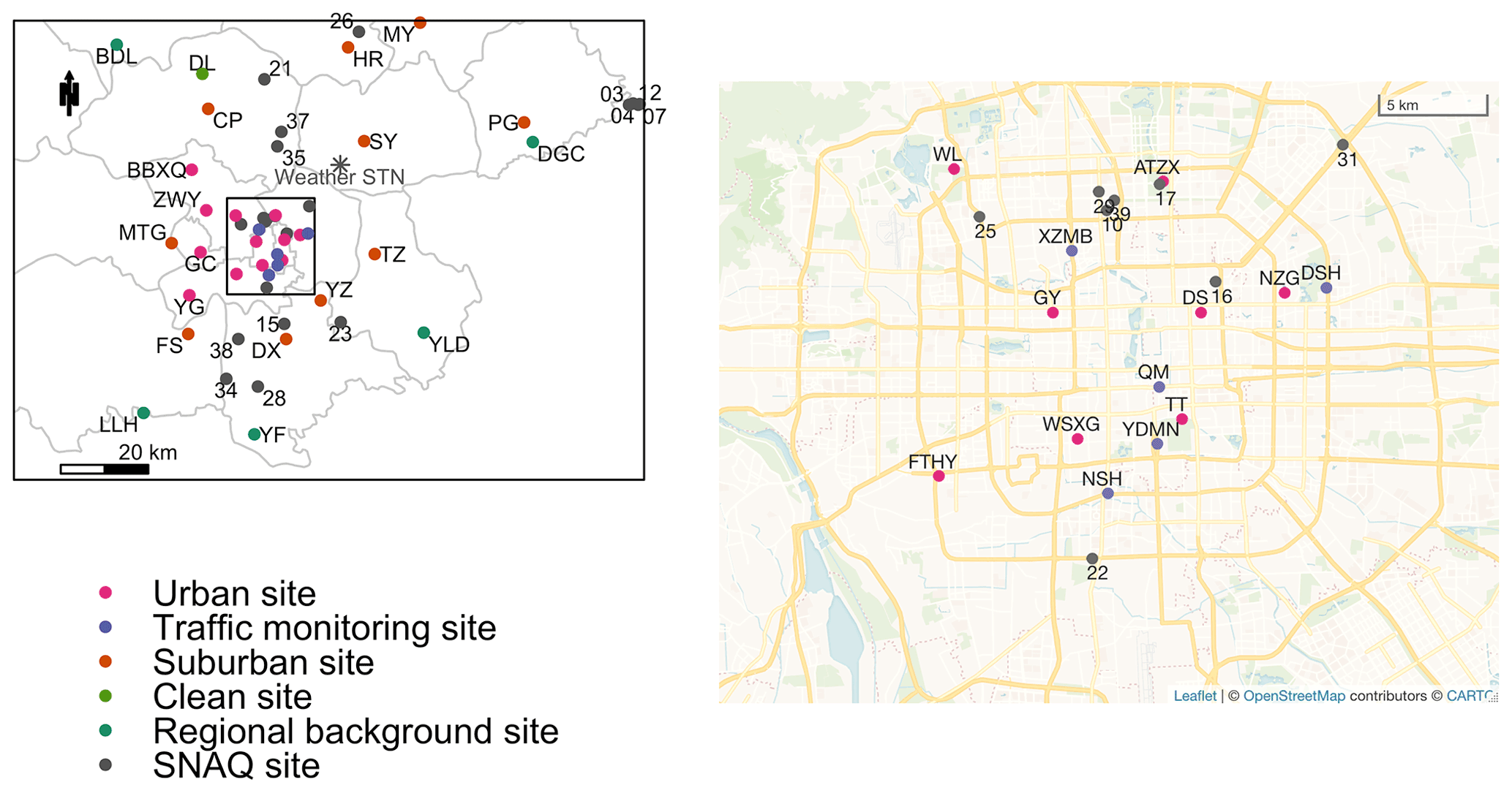
Figure 1 The modelling domain as set by the extent of the base emissions (see Sect. 2.2) with the locations of air quality measurements used in this study, including a magnified view of the area within the 5th Ring Road of Beijing (right panel). Long-term monitoring sites are colour-coded according to the site type and labelled by their acronyms. Full names and coordinates are listed in Table S1. Locations of low-cost sensor (SNAQ) measurements are shown in dark grey, and the coordinates can be found in Table S2. The weather station where the input meteorological observations were made is marked by the grey star symbol. The administrative divisions of Beijing are shown by light grey outlines.

In addition, we used high-frequency (20 s) measurements of NO, NO₂ and O₃ from November–December 2016, the winter campaign period of the Atmospheric Pollution & Human Health in a Chinese Megacity (APHH-Beijing) research programme (Shi et al., 2019). The measurements were made with low-cost sensors also deployed in a variety of near-surface locations in Beijing (with an average measurement height of 8 m) and are hereinafter referred to as SNAQ (Sensor Network for Air Quality) (Fig. 1 and Table S2). The dataset has been validated against reference instrument measurements also obtained during the campaign and those from the aforementioned long-term monitoring sites.

2.2 Perturbed emissions ensemble

We used a special version of the Multi-resolution Emission Inventory for China (MEIC) v1.3 (Li et al., 2017; Zheng et al., 2018) developed for use in the APHH-Beijing programme. The inventory characterises emissions of CO, NO_x (and NO₂), total VOC (TVOC), SO₂, PM₁₀ and PM_2.5 from the industry, power, residential and transport sectors in 2013. It extends 120 and 150 km in the north–south and east–west directions, respectively, covering most of Beijing and parts of Hebei Province with 3 km × 3 km horizontal resolution. In the vertical, there are seven layers with the top of each layer at 38, 90, 152, 228, 337, 480 and 660 m above ground, respectively. Each source sector is associated with a specific set of diurnal, monthly and vertical variation profiles that is applied to emissions of all pollutants from the sector. This inventory has been used to simulate street level air quality (Biggart et al., 2020) and quantify regional pollution transport (Panagi et al., 2020) and has been compared with direct flux measurements (Squires et al., 2020). To focus on locations where observations were available, we cropped the original extent to a smaller region of 105 km × 144 km (starting from the Northwest) and used it as the a priori emissions, hereinafter referred to as the base emissions. Annual NO_x emissions in this region are shown in Fig. S1 by source sector.

NO_x and TVOC emissions in Beijing were reported to have decreased substantially between 2013 (the year of the emission estimates) and 2016, when the observations were made (Cheng et al., 2019; Xue et al., 2020). In the surrounding provinces, NO_x emissions also revealed a downward trend, while no apparent trend has been identified for TVOC emissions (Zheng et al., 2018). In addition to spatial disparities, emissions from individual source sectors also showed different patterns. In Beijing, for example, vehicle emission control contributed the most NO_x reductions, while the largest TVOC decrease was found in the petrochemical industry (Cheng et al., 2019; Xue et al., 2020). Hence, uncertainties associated with the NO_x emissions from each sector in the base emissions were estimated separately. Due to a lack of long-term observations, uncertainties associated with the TVOC emissions were not investigated, the impact of which on the constrained NO_x emissions is discussed in Sect. 4.

Table 1 Emission parameters^a and the respective uncertainty ranges sampled by the initial and the adjusted perturbed emissions ensembles (PEEs). n/a – not applicable.

^a All parameters are defined as ratios of the 2016 emissions to the base emissions from 2013, except for the night-time fraction of transport sector NO_x emissions which is defined as a percentage (%) of the daily totals in 2016. ^b Power sector NO_x emissions are effectively represented by one parameter in the initial PEE. In the adjusted PEE, the emissions are split into two parameters, namely emissions below and above 152 m. ^c Night-time fraction of transport sector NO_x emissions is defined as those occurring during 23:00–06:00 LT in the initial PEE. In the adjusted PEE, it is modified to NO_x emitted during 00:00–05:00 LT from the transport sector.

To reduce subjectivity, the uncertainties were determined based on elicitation of expert knowledge. Table 1 shows the NO_x emission parameters investigated. To facilitate the expert elicitation and the subsequent construction of PEEs, the parameters were defined as ratios of the 2016 values to the corresponding 2013 estimates in the base emissions. An exception is the last parameter which represents the night-time fraction (in percentage) of transport sector NO_x emissions in 2016, irrespective of that in 2013. It allowed for perturbations to the diurnal distributions of traffic NO_x emissions on top of perturbations to the total magnitude. In the initial PEE (see below and Sect. S1), the night-time fraction was defined as emissions occurring between 23:00 and 06:00 local time (UTC+8) (inclusive) following Biggart et al. (2020), who provided evidence of an underestimation in the night-time vehicle sources of NO_x in the a priori emissions inventory. This was attributed to an underrepresentation of emissions from heavy duty diesel trucks, which typically travel from surrounding provinces into Beijing at night, as they are banned from entering the central urban areas during the day. After reviewing a previous study which summarised the varying traffic rules and restrictions for different types of vehicles in Beijing (Zhang et al., 2019), the definition was modified to traffic NO_x emitted during 00:00–05:00 LT (inclusive) for the adjusted PEE.

To simultaneously perturb the total magnitude and the vertical distribution of emissions, the three-dimensional industry sector was split into two parameters, namely ground-level emissions (i.e. from the lowest vertical layer) and elevated emissions (i.e. from all upper layers). This was also intended for the power sector. However, as emissions from the sector are present in all but the lowest layer, their vertical variation profile was effectively unchanged in the initial PEE. The issue was fixed by introducing two new parameters for power sources below and above 152 m (top height of the fourth vertical layer), respectively, for the adjusted PEE. Residential and transport emissions are only found in the ground layer and were thus represented each by a single parameter.

An online questionnaire was designed for the elicitation (available at https://cambridge.eu.qualtrics.com/jfe/form/SV_3eGxf9XvC7WXESV, last access: 14 April 2022) and circulated via the mailing list of the APHH-Beijing programme. A total of seven responses was received. Despite constituting a relatively small group, the participants included researchers with expertise in compiling an emissions inventory for the region of interest and researchers who used the same a priori emissions inventory in their own work. The fact that their responses were largely consistent also backs the credibility of the results. Specifically, the participants were invited to advise a lower and an upper bound of uncertainty for each emission parameter, such that it would be very unlikely for the true value to fall outside this range. The responses from the first round of elicitation were sent back to the participants anonymously for review. Finally, the maximum and minimum values advised by all participants for each parameter in the second round were adopted (Table 1, “Initial PEE” column). These wide uncertainty ranges also compensated for the small size of the expert group.

Model simulations using the initial PEE as inputs showed substantial overestimation of NO₂ concentrations, such that many members of the ensemble were unusable for constraining the emissions (see Sect. S1). Hence, we designed an adjusted PEE by decreasing the elicited lower bounds of uncertainty for all parameters concerning the magnitude of NO_x emissions from a certain source sector. The upper bound of uncertainty for the transport emissions was also reduced, as the modelled diurnal concentration profiles indicated positive biases linked specifically to the sector. Lastly, the uncertainty range of the night-time fraction of transport emissions was adjusted following the new definition described above (Table 1, “Adjusted PEE” column).

As this study also sought to improve emission estimates of CO in the base emissions (the results of which are presented in Yuan et al., 2021), the uncertainty ranges of relevant emission parameters were also elicited and modified in the same processes as the NO_x emission parameters. The 14 parameters in total (i.e. 7 for NO_x, 7 for CO) determined for the adjusted PEE constituted a 14-dimensional uncertain space, which was probed efficiently using the maximin Latin hypercube sampling, which maximises the minimum inter-sample distance (Johnson et al., 1990). A rule of thumb is to have a sample size 10 times the dimension (Loeppky et al., 2009). We drew 140 samples, effectively doubling the sample size generally required (i.e. if only NO_x emission parameters were perturbed). A simultaneous perturbation to both CO and NO_x was justified by the fact that CO is treated as an inert pollutant in the model used (see Sect. 2.3); thus varying CO emissions do not affect the modelled NO_x concentrations (and vice versa). The sample values were then used as spatio-temporally uniform scaling factors to perturb the corresponding values in the base emissions to construct a 140-member PEE, hereinafter referred to as the adjusted PEE. Figure 2 shows the total NO_x emissions by source sector and vertical layer and the mean diurnal variations of NO_x emissions in the ensemble members. In each member, the set of scaling factors applied to NO_x was also applied to the emissions of NO₂, such that primary NO₂ (f-NO₂, i.e. the proportion of NO_x emitted directly as NO₂) in the base emissions remained unchanged, with a value of 6.7 % in all source sectors (and thus grid cells). In reality, however, the f-NO₂ varies between sectors. Much attention has been paid to the f-NO₂ in vehicle exhausts, while little is known about the f-NO₂ in residential emissions. It is thus difficult to evaluate whether the 6.7 % in the base emissions is representative of the aggregated NO_x emissions in the study area.

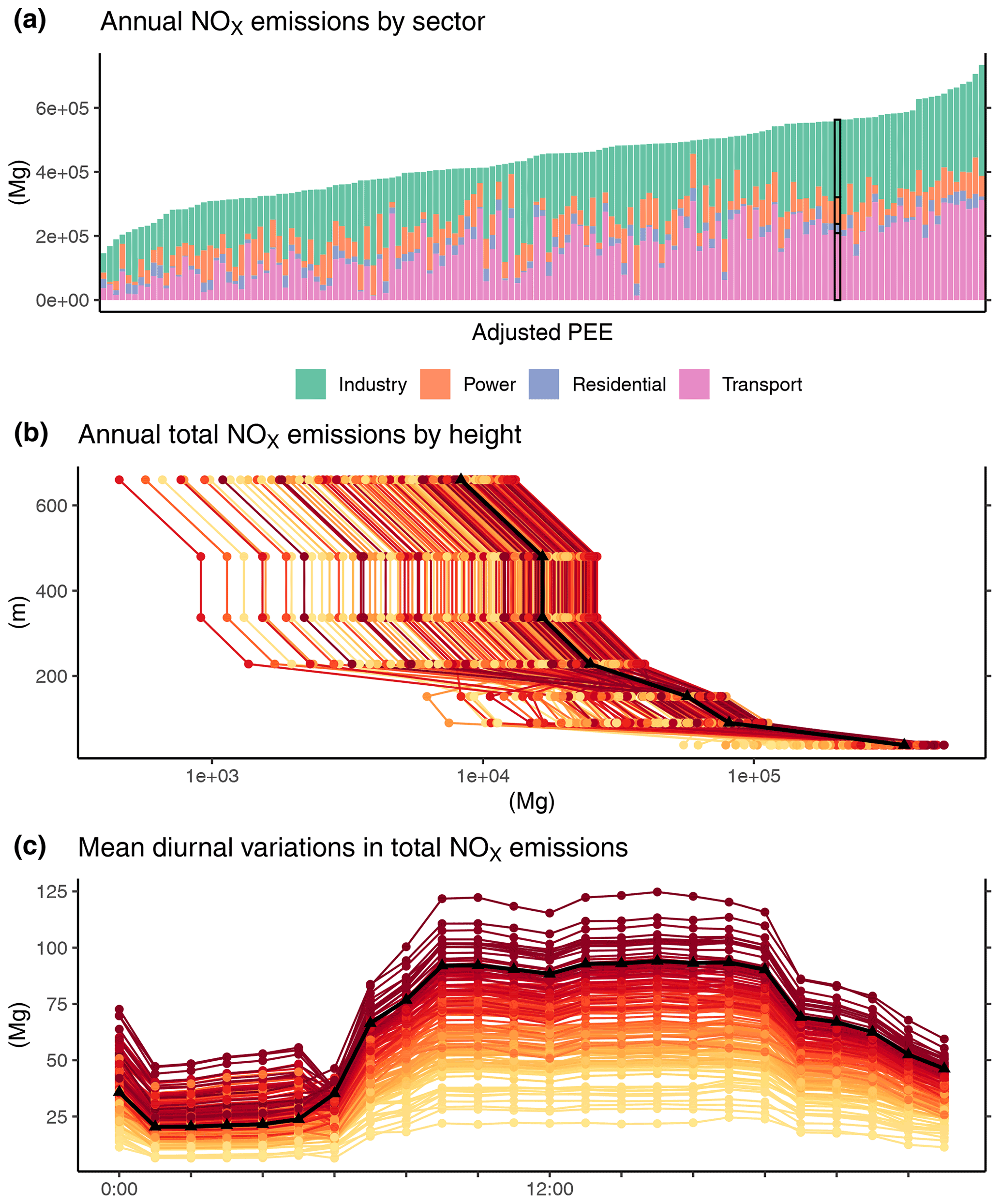
Figure 2 (a) Annual total NO_x emissions shown by contributions from individual source sectors in the 140-member adjusted perturbed emissions ensemble (PEE) and the base emissions (marked by black frames). (b) Vertical distributions of the annual total NO_x emissions in the adjusted PEE and the base emissions. The height represents the top height (above local ground level) of each vertical layer. (c) Annual mean diurnal variations (in local time) in total NO_x emissions in the adjusted PEE and the base emissions. In panels (b) and (c), the base emissions are marked by black lines and triangle symbols, while the adjusted PEE members are colour-coded according to their annual total NO_x emissions, with darker colours indicating higher values.

2.3 Model description and simulation setup

We used ADMS-Urban (version 4.2), a state-of-the-art urban-scale high-resolution quasi-Gaussian dispersion model (McHugh et al., 1997; Owen et al., 2000). The model has been applied in air quality simulations in cities worldwide including Beijing (Biggart et al., 2020; He et al., 2019; Hood et al., 2018). Dispersion calculations are based on the state of the atmospheric boundary layer, which is parameterised based on Monin–Obukhov similarity theory (Venkatram, 1996). The parameterisation is explained in detail in previous studies (e.g. Biggart et al., 2020). The minimum required meteorological input data including hourly wind speed, wind direction and cloud cover were measured at a weather station at Beijing Capital International Airport (see Fig. 1) and archived in the NOAA Integrated Surface Database (Smith et al., 2011). Local disturbance to the mean flow field by individual buildings and street canyons was not accounted for as such data were unavailable. Nonetheless, differences in the near-surface dynamics at the weather observatory (situated in open landscape) and at the measurement sites (the majority of which are located in built-up areas) were represented by different values of roughness length and minimum Obukhov length, as described in Yuan et al. (2021).

Chemistry calculations are enabled by two fast chemistry schemes for the NO_x photolytic chemistry and the formation of sulfate aerosols, respectively (Cambridge Environmental Research Consults Limited, 2017). The former is based on the Generic Reaction Set (Azzi et al., 1992) which reduces the complex mechanisms involving NO_x, O₃ and VOCs to seven reactions:

$$\begin{array}{}\text{(R1)}& {\displaystyle }\mathrm{ROC}+h\mathit{\nu }\to \mathrm{RP}+\mathrm{ROC}\text{(R2)}& {\displaystyle }\mathrm{RP}+\mathrm{NO}\to {\mathrm{NO}}_{\mathrm{2}}\text{(R3)}& {\displaystyle }{\mathrm{NO}}_{\mathrm{2}}+h\mathit{\nu }\to \mathrm{NO}+{\mathrm{O}}_{\mathrm{3}}\text{(R4)}& {\displaystyle }\mathrm{NO}+{\mathrm{O}}_{\mathrm{3}}\to {\mathrm{NO}}_{\mathrm{2}}\text{(R5)}& {\displaystyle }\mathrm{RP}+\mathrm{RP}\to \mathrm{RP}\text{(R6)}& {\displaystyle }\mathrm{RP}+{\mathrm{NO}}_{\mathrm{2}}\to \mathrm{SGN}\text{(R7)}& {\displaystyle }\mathrm{RP}+{\mathrm{NO}}_{\mathrm{2}}\to \mathrm{SNGN}\text{(R8)}& {\displaystyle }\mathrm{2}\mathrm{NO}+{\mathrm{O}}_{\mathrm{2}}\to \mathrm{2}{\mathrm{NO}}_{\mathrm{2}},\end{array}$$

where ROC, RP, SGN and SNGN represent reactive organic compounds, radical pool, stable gaseous nitrogen product and stable non-gaseous nitrogen product, respectively. Reaction (R8) has been added to the scheme in ADMS-Urban, but its impact is only significant with sustained high levels of NO concentrations (e.g. 1000 µg m⁻³ for several hours) due to a small rate constant (Cambridge Environmental Research Consults Limited, 2017). It is evident that only Reactions (R3) and (R4) are conservative chemical reactions, while the rest represent approximations of multiple reactions lumped together. For example, Reaction (R1) represents all reactions that produce radicals via the photo-oxidation of VOCs. Thus, the rate coefficients of these generic reactions have been determined empirically by fitting the simulation outputs to smog chamber data (Azzi et al., 1992). The rate constant of the explicit reaction, Reaction (R3), can be calculated from solar radiation, which is often estimated by ADMS-Urban based on the input meteorological data, when direct measurements are unavailable (as is the case in this study). By appealing to NO_x–O₃ photostationary state, the model also derives a NO₂ photolysis rate from the background concentrations of NO, NO₂ and O₃ and takes the lower value between the two (Cambridge Environmental Research Consults Limited, 2017).

Background pollutant concentrations are thus required as an input, not only to account for pollution sources not included in the input emissions (e.g. transported from outside the extent of the emissions inventory), but also to constrain the reaction coefficients for reactive species. As mentioned in Sect. 2.1, continuous measurements of NO₂ and O₃ are available from the long-term monitoring network. In each hour, we input the inverse-distance-weighted mean of the concentrations at two of the clean or regional background sites (a total of six; see Fig. 1) located to each side of the incoming wind direction in that hour as the background in the adjusted PEE simulations. This was different from the initial PEE simulations (see Sect. S1) which used a baseline concentration, defined as the 10th percentile of the concentrations from all sites in a moving 3 h window. The method of using a network baseline to represent the non-local pollution signal has previously been applied to CO, which is inert in ADMS-Urban (Yuan et al., 2021) and NO_x and O₃ at a small spatial scale (Popoola et al., 2018). At larger scales, however, though it has been established that concentrations of total oxidants (O_x = O₃ + NO₂) consist of a local component that correlates with NO_x emissions and a NO_x-independent regional component (Clapp and Jenkin, 2001; Han et al., 2011), the partition of O_x between NO₂ and O₃ may be highly variable in time and space due to their rapid interconversion and reactions with other species. Using values measured at two neighbouring sites away from major sources ensured a more realistic partition of O_x in the adjusted PEE simulations. The sensitivity of the simulation output to different definitions of NO₂ and O₃ background concentrations is further investigated in Sect. 4.

For NO and TVOC for which long-term measurements were unavailable, we used upwind concentrations from the Copernicus Atmosphere Monitoring Service (CAMS) reanalysis dataset (Inness et al., 2019). At each time step (every 3 h), we calculated the inverse-distance-weighted mean of the values from the two grid cells in the lowest vertical layer located directly outside of the modelling domain and to each side of the incoming wind. The time series obtained was then linearly interpolated to hourly resolution, as required by ADMS-Urban. As TVOC is not a standard output variable in the dataset, a sum of the eight available VOC species was used to approximate TVOC. To validate this approach, we compared the sum of mixing ratios of 29 VOC species measured at the Institute of Atmospheric Physics, Chinese Academy of Sciences during the APHH-Beijing winter campaign with the approximate TVOC mixing ratios from the corresponding grid cell in the reanalysis product during the same period. Apart from a few peak events not seen in the latter, the two time series show a good level of agreement, both in terms of the trend and the magnitude (Fig. 3a). The upwind NO mixing ratios extracted from the CAMS reanalysis dataset were compared to NO baseline mixing ratios extracted from the SNAQ measurements. Figure 3b shows a substantial positive bias in the NO extracted from the reanalysis dataset, the cause of which remains unknown. To prevent this bias from being propagated into the modelled concentrations, a bias correction was applied using empirical quantile mapping. This method equates the (empirically estimated) cumulative distribution functions (i.e. quantile functions) of the modelled and observed time series for regularly spaced quantiles (Boé et al., 2007; Cannon et al., 2015). During the campaign period, this significantly reduced the bias, while the correlation was only slightly decreased. However, larger uncertainties would have been introduced when the transfer function was extrapolated to the entire time series of 2016, which were unavoidable and difficult to quantify due to a lack of long-term measurements. Yet these were likely smaller than the uncertainties associated with using the uncorrected, positively biased values obtained from the CAMS reanalysis product.

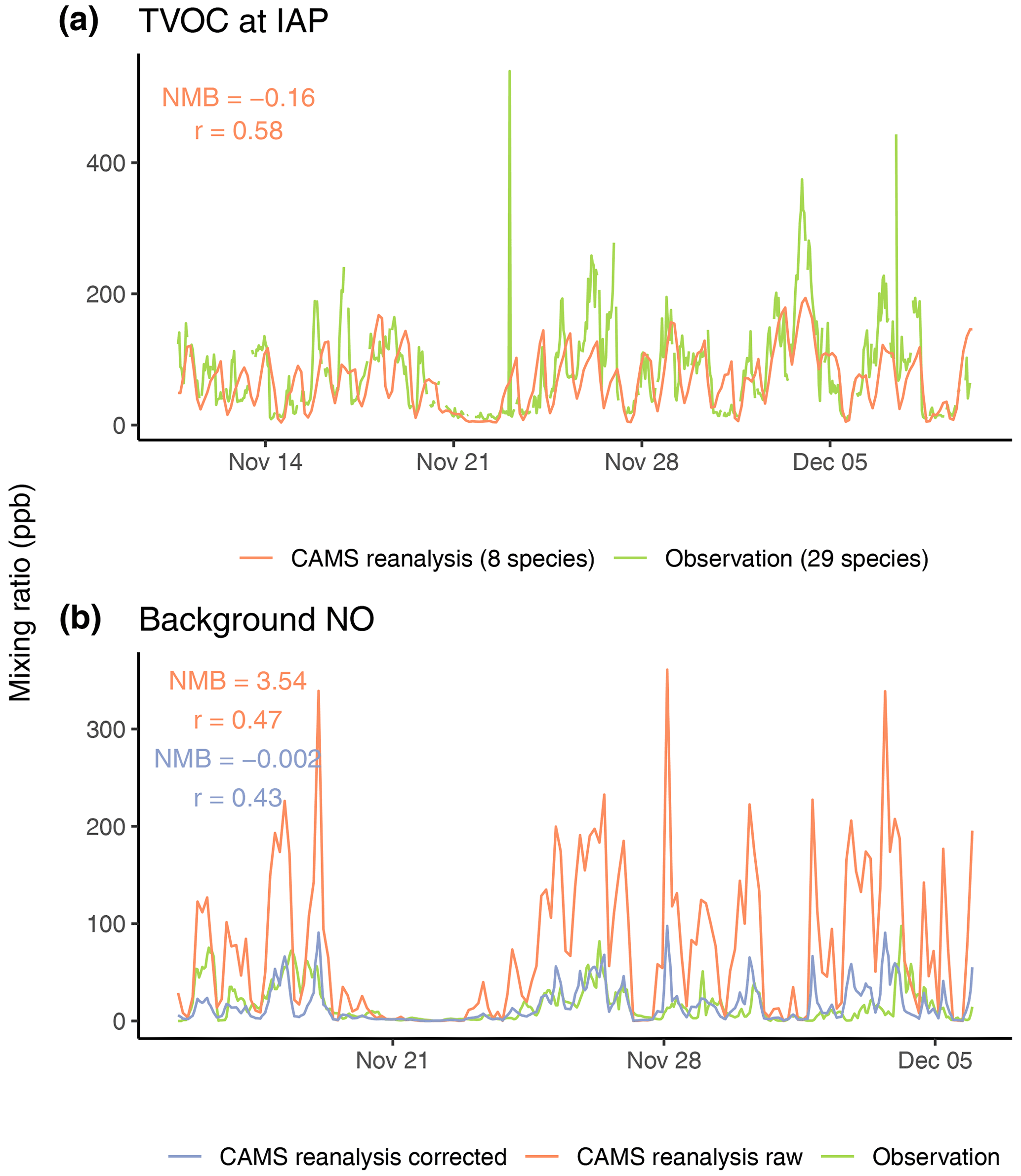
Figure 3 (a) Mixing ratios of TVOC at the Institute of Atmospheric Physics (IAP), Chinese Academy of Sciences, during the APHH-Beijing winter campaign from the Copernicus Atmosphere Monitoring Service (CAMS) reanalysis dataset, compared to observations. TVOC from the reanalysis product was approximated by the sum of eight available VOC species. The observed TVOC was calculated as the sum of 29 VOC species measured. (b) Original and bias-corrected upwind mixing ratios of NO from the reanalysis dataset (the latter were input as background pollution levels in the PEE simulations), compared to baseline (10th percentile) mixing ratios from the SNAQ measurements. For each reanalysis time series, the data and the normalised mean bias (NMB) and Pearson's correlation coefficient (r) are shown in the same colour.

The input meteorology data and background pollutant concentrations described above provided the same lateral boundary conditions for the 140 adjusted PEE simulations, among which only the emissions of NO_x (and NO₂) varied. An additional simulation forced with these boundary conditions and the base emissions was also performed and is hereinafter referred to as the base run. All 141 simulations were run for the whole year of 2016 to produce hourly pollutant concentrations at each measurement location (see Fig. 1). Output of these simulations was then compared to measurements to derive a posteriori emission estimates.

3 Results

We first evaluated the performance of the adjusted PEE simulations in modelling NO₂ concentrations at the long-term monitoring sites using mean square error (MSE). It is a compact indicator of model performance whose merit is demonstrated in the following. The MSE is calculated as

$$\begin{array}{}\text{(1)}& \mathrm{MSE}={\displaystyle \frac{\mathrm{1}}{n}}{\sum }_{i=\mathrm{1}}^n{\left({\mathrm{mod}}_i-{\mathrm{obs}}_i\right)}^{\mathrm{2}},\end{array}$$

where obs_i is the observed value for a given averaging period i (e.g. an hour, a day, a month), mod_i is the corresponding simulation output and n represents the number of the available observations.

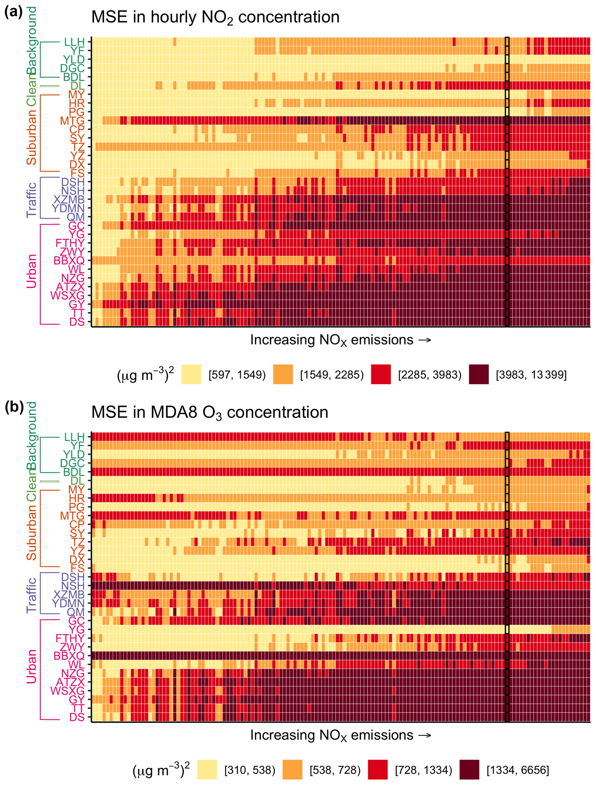
Figure 4 Mean square errors (MSEs) in (a) hourly NO₂ concentrations and (b) daily maximum 8 h mean (MDA8) O₃ concentrations associated with the adjusted perturbed emissions ensemble (PEE) simulations, arranged in ascending order of the input annual total NO_x emissions (from left to right) and the base run (marked by black frames) at each long-term monitoring site. In each panel, the MSEs are grouped into quartiles and colour-coded accordingly. The monitoring sites are arranged and colour-coded according to the site type: urban site (magenta), traffic monitoring site (purple), suburban site (orange), clean site (light green) and regional background site (green).

At each site, MSE is calculated for the hourly NO₂ concentration output by each adjusted PEE simulation and the base run. Figure 4a shows a distinct trend of increasing MSEs with growing annual total NO_x emissions, such that at most sites, the base run with input emissions at the upper end of the scale (see Fig. 2a) is outperformed by most of the PEE simulations. Although a single MSE does not differentiate between over- and underestimation, this clear positive association between MSEs and NO_x emissions suggests that NO_x emissions are positively biased, both in the base emissions and in most members of the PEE. If NO_x emissions were negatively biased in a considerable subset of the ensemble members, the MSEs would first decrease as emissions increased, until the absolute bias in the emissions reached a minimum. It is also evident that the base run is generally associated with larger errors at urban and traffic monitoring sites compared to other sites. Moreover, the increase in MSEs with increasing emissions is more rapid at these locations, resulting in a wider range of errors associated with the ensemble of simulations. This is an indication that the base emissions are larger in magnitude in the central areas (where these sites are situated; see Fig. 1) than in the periphery and are overestimated to a larger extent. Though spatially uniform scaling factors were applied within the study area, regions with higher base emissions would show larger variations in the perturbed emissions and thus model errors. This highlights a potential issue associated with spatially uniform perturbations to spatially non-uniform emissions.

Due to the important role of O₃ in converting NO into NO₂, the adjusted PEE simulations' performance in modelling the O₃ concentrations was also evaluated. In other words, this was to ensure that the underlying chemical mechanisms were correctly modelled and that simulations with lower NO_x emissions showed better agreement with NO₂ observations for the right reasons. We calculated the MSEs in maximum daily 8 h mean (MDA8) O₃ concentrations¹. Among the numerous O₃ metric available, the MDA8 O₃ is widely used for model–observation comparison due to its relevance in regulation and health impact assessments (Lefohn et al., 2018). Figure 4b shows that as with NO₂, the base run is also generally associated with higher MSEs than many PEE simulations. At more sites, however, the positive association between model error and NO_x emissions seen in Fig. 4a breaks down (e.g. at DSH and MTG) or even becomes reversed (e.g. at HR and LLH). This underscores the complex effects of non-linear chemistry and suggests that the MSEs in MDA8 O₃ are less strongly associated with the input NO_x emissions, the reason for which can be revealed by a breakdown of the MSE.

The MSE can be mathematically decomposed into the sum of three terms (Solazzo and Galmarini, 2016):

$$\begin{array}{}\text{(2)}& \begin{array}{rl}\mathrm{MSE}& =\left[{\left(\stackrel{\mathrm{‾}}{\mathrm{mod}}-\stackrel{\mathrm{‾}}{\mathrm{obs}}\right)}^{\mathrm{2}}\right]+\left[{\left({\mathit{\sigma }}_{\mathrm{mod}}-r{\mathit{\sigma }}_{\mathrm{obs}}\right)}^{\mathrm{2}}\right]\\ & +\left[{\mathit{\sigma }}_{\mathrm{obs}}^{\mathrm{2}}\times \left(\mathrm{1}-r^{\mathrm{2}}\right)\right],\end{array}\end{array}$$

where σ_mod and σ_obs represent the standard deviation of the modelled and observed values, respectively, and r is the Pearson's correlation coefficient between model outputs and observations. The first term in Eq. (2) represents the bias component of model error, and it is largely introduced by external forcings, for example, input emissions and boundary conditions. The second term is the variance error which is associated with the processes resolved in a model. A trade-off between bias and variance, in other words, accuracy and precision, is often inevitable in complex models (Sun and Archibald, 2021). The last term, by definition, represents the proportion of the observed variance unexplained by the model. It summarises all non-systematic errors, including the noise and inherent variability (e.g. due to turbulence closure) in the observations as well as errors arising from the linearisation of non-linear processes and is referred to as the minimum achievable MSE (mMSE). The MSE is thus a well-rounded metric suitable for operational model evaluation, and its decomposition provides indications of possible sources of model error (Solazzo and Galmarini, 2016).

Figure 5 Error component with the highest contribution to the mean square errors (MSEs) in (a) hourly NO₂ concentrations and (b) daily maximum 8 h mean (MDA8) O₃ concentrations associated with the adjusted perturbed emissions ensemble (PEE) simulations, arranged in ascending order of the input annual total NO_x emissions (from left to right) and the base run (marked by black frames) at each long-term monitoring site. The monitoring sites are arranged and colour-coded according to the site type: urban site (magenta), traffic monitoring site (purple), suburban site (orange), clean site (light green) and regional background site (green).

The values of MSEs shown in Fig. 4 were decomposed according to Eq. (2), and the term with the largest contribution to the MSE associated with each simulation at each site is shown in Fig. 5. There are striking differences in the attribution of error for hourly NO₂ and MDA8 O₃. Variance errors have the largest share in the MSEs in hourly NO₂ concentrations associated with most of the adjusted PEE simulations at over half of the reference sites. At another $\mathrm{1}/\mathrm{4}$ of the sites, all of which are urban or traffic monitoring sites, bias accounts for most of the errors in the bulk of the simulations. This is another indication of a higher degree of overestimation in the central areas in the base emissions and subsequently in many members of the adjusted PEE. For most sites (regardless of the site type), simulations using the lowest annual total NO_x emissions are associated with MSEs that are mostly made up by the mMSE.

At the urban and traffic monitoring sites where the MSEs in hourly NO₂ associated with the ensemble simulations are mainly made up of the bias error, the bias also happens to be the largest term in most MSEs in MDA8 O₃ (Fig. 5b). At most other sites (including all suburban, clean and regional background sites), however, the MSEs in MDA8 O₃ are dominated by the mMSE, irrespective of the input NO_x emissions. This explains the weaker association between the total MSEs in MDA8 O₃ and the emissions revealed in Fig. 4b, as the mMSE is much less dependent on model inputs. A further breakdown of the mMSEs (Fig. S4) reveals that variances in the observations of MDA8 O₃ are substantially higher than those in the observed hourly NO₂ concentrations. Despite considerably better correlation between model outputs and the observations, these large variances in the observations result in mMSEs in MDA8 O₃ concentrations that are only moderately smaller than those associated with hourly NO₂ concentrations. Meanwhile, the MSEs in O₃ are considerably lower than those in NO₂; the largest share of the mMSEs in the former is thus explained. Because of this dependence on the observations and the weaker connection to external drivers, the mMSE is often considered the least concerning component of model error (Solazzo and Galmarini, 2016).

Figure 6 Decomposed median mean square errors (MSEs) in (a) hourly NO₂ concentrations and (b) daily maximum 8 h mean (MDA8) O₃ concentrations associated with the adjusted perturbed emissions ensemble (PEE) simulations, arranged in ascending order of the input annual total NO_x emissions (from left to right) and the base run (marked by black frames).

As the distributions of the 33 MSEs (i.e. one for each long-term monitoring site) associated with individual PEE simulations are mostly non-Gaussian, we used the median MSE to represent a simulation's average performance for a certain pollutant across all sites within the modelling domain. A breakdown of the median MSEs (Fig. 6) is consistent with the findings described above: with more accurate (lower) input NO_x emissions, a simulation's average performance for hourly NO₂ can be improved substantially to a point that the remaining model error consists mostly of the non-systematic mMSE. The average performance for MDA8 O₃ is less strongly associated with NO_x emissions, as it is dominated by the mMSE in the majority of the PEE simulations. These associations between median MSEs and input emissions are also tested using simple linear regression (Fig. S5). Though both regression models are statistically significant (p value < 0.001), more variability in the modelled hourly NO₂ is explained, compared to that in the modelled MDA8 O₃. The scatter of the points around the regression line reveals the variations in model performance with varying mix of source sectors, given similar strengths of total emissions (note that these are represented on an ordinal scale in Figs. 4–6). This also demonstrates the importance of using network observations as constraints. With spatially uniform perturbations, it is likely that several different combinations of emission parameter values result in similar concentrations at a particular location. The risk of constraining the parameter values to just one of the possible combinations is reduced, when observations that sample a wide range of local environments are used.

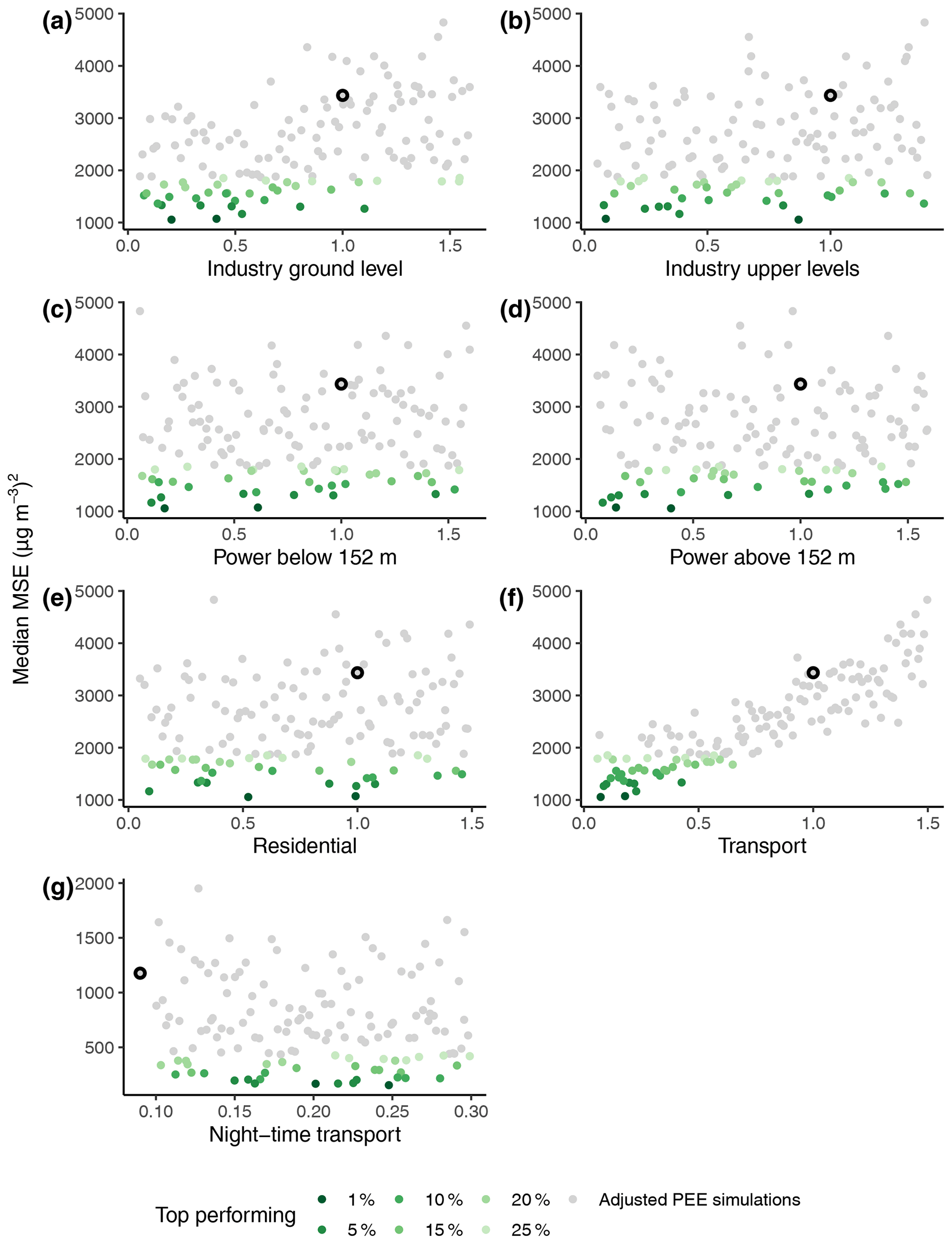
Figure 7 Average performance of the adjusted perturbed emissions ensemble (PEE) simulations and the base run (marked with black strokes) as a function of emission parameter values. The scales on the x axes correspond to the uncertainty ranges in Table 1, “Adjusted PEE” column. The top-performing 25 %, 20 %, 15 %, 10 %, 5 % and 1 % of the simulations are coloured in a darkening green shade, as measured by their median mean square errors (MSEs) in hourly NO₂ concentrations at the long-term monitoring sites across the modelling domain (see Fig. 6) in all panels except in panel (g), where median mean square errors in the annual mean diurnal variations of NO₂ concentrations are used (note the different scale on the y axis).

On account of the analysis above, we only used observations of NO₂ to constrain NO_x emissions, which is also in line with numerous top-down emission optimisation studies using satellite observations of column NO₂ (Lamsal et al., 2011; Martin et al., 2003; Napelenok et al., 2008; Qu et al., 2017). Figure 7 shows the average performance for hourly NO₂ of individual PEE simulations against the value set for each emission parameter in Table 1. Figure 7f reveals a strong positive correlation between the median MSE in hourly NO₂ of a simulation and the input transport sector NO_x emissions. Simulations with a median MSE within the first quartile are forced with transport emissions 6 %–65 % of those in the base emissions. This range continues to reduce (from both ends) with improving simulation performance, such that when the median MSE falls below the 10th percentile, the corresponding traffic emissions are only 7 %–43 % of those in the base emissions. The range determined by the top-performing 5 % of the simulations (i.e. with a median MSE within the fifth percentile) remains the same, while it can be further constrained one-sidedly to 7 %–18 % if only the top 1 % were considered. However, as the top 1 % of a 140-member ensemble contains (maximally) two simulations, the difference in whose average performance is marginal (≤ 1.5 %), this range was considered not robust.

In addition to the total magnitude, the night-time fraction of the transport sector NO_x emissions could also be constrained (Fig. 7g). Instead of hourly NO₂, performance of the adjusted PEE simulations was evaluated against the observed annual mean diurnal variations of NO₂ at each long-term monitoring site. The median of all 33 MSEs in the diurnal profiles at individual sites modelled by a simulation was also used to represent its average performance in modelling the different diurnal profiles observed within the study area (see Fig. S3). Though not as evident as the case of total transport emissions, the range of the night-time fraction also becomes narrower with improving model skill. Amongst simulations with a median MSE in diurnal NO₂ profiles within the 15th percentile, 11 %–29 % of the transport emissions occur at night (in contrast to the 9 % in the base emissions). In the top 5 % of the simulations, this fraction varies between 15 % and 25 %.

Emission parameters for other source sectors could not be constrained with strong confidence (Fig. 7a–e), as the ranges of parameter values only start to noticeably differ from the full uncertainty range when the median MSE in hourly NO₂ falls within the 10th percentile or even below. The residential sector is the smallest source sector of NO_x in the base emissions (see Fig. 2a). A source apportionment of the base run reveals that its contribution to the annual mean NO_x concentrations at individual long-term monitoring sites varies between 3 % and 8 % (Fig. S6). It can thus be expected that even a 150 % increase, i.e. its upper bound of uncertainty (see Table 1, “Adjusted PEE” column), is not sufficient to cause substantial changes in the simulation performance for NO_x, based on which the emissions can be constrained.

Interestingly, Fig. S6 also reveals that at most sites, the contribution of NO_x base emissions from the power sector to the modelled annual mean NO₂ concentrations is even smaller than that from the residential sector, though the emissions are over 2 times higher (see Fig. 2a). This is attributable to the nature of the power sector, which is characterised by a few large point sources emitting at elevated levels. These sources undergo greater dispersion before reaching the surface-based monitoring sites (compared to ground-level emissions); thus their impact at most sites is small. As an example, the annual mean NO_x concentration simulated at the site NZG is very similar to that modelled at the site GC, yet less than 3 % of this concentration stems from NO_x emissions from the power sector, as opposed to the 11 % share at GC (Fig. S6). This can be explained by Fig. S7 in which the concentration resulted from power emissions is further apportioned to each grid cell. It is evident that the concentration at GC is predominantly contributed by the grid cell directly to its west. In fact, this grid cell contains the highest power emissions of NO_x within the study area. In comparison, the site NZG is located at some distance from other grid cells with relatively large power sources. The contributions of these grid cells to the NO_x concentrations at NZG are smaller. The differences are about 1 order of magnitude, as the contributions are log-transformed in the figure.

The fact that emissions released at higher levels are not well sampled by the existing surface-based monitoring sites also applies for those of NO_x from industrial sources (emitted at up to 152 m). In addition, emissions from both source sectors were separated into two parameters and perturbed simultaneously (i.e. in an uncorrelated matter) for varying vertical distributions. The uncertainty range of the sum of the two parameters, i.e. the total power or industrial emissions, was thus smaller than the individual uncertainty ranges and may not be sufficiently large to capture the actual emissions.

The short-term, independent SNAQ measurements of NO₂ were also used to constrain the emission parameters following the same approach (Fig. S8). Similarly, adjusted PEE simulations showing better performance for hourly NO₂ concentrations and mean diurnal variations of NO₂ concentrations (over the measurement period) at SNAQ sites are associated with lower transport sector total emissions, but a higher percentage of these emissions occur at night. In the top-performing 5 % of the simulations, total traffic emissions are 7 %–43 % of those in the base emissions, while the night-time fraction varies between 15 % and 26 %. The fact that the uncertainty ranges constrained by the short-term SNAQ measurements are consistent with those using long-term reference measurement demonstrates the robustness of both this approach and the findings. This also supports the use of low-cost sensors for this particular application, as they are more affordable for deployment in a dense network.

4 Discussion

According to the base emissions, total NO_x emissions from the transport sector were 2.1 × 10⁵ Mg within the study area which extends over most of Beijing and parts of Hebei Province in 2013, 9 % of which occurred during 00:00–05:00 LT. Based on the top 5 % of the adjusted PEE simulations for modelling NO₂ hourly concentrations and diurnal profiles, we found that transport NO_x emissions were likely to have decreased to 1.5–9 × 10⁴ Mg (i.e. a 57 %–93 % reduction) in 2016, and the night-time fraction was between 15 % and 25 %.

An exact comparison of these results with findings of previous studies is not possible, as the emissions were investigated over different spatial and/or temporal scales. However, it is possible to compare the relative changes in emissions. Biggart et al. (2020) found that total NO_x emissions rates from the same a priori emissions inventory (and all source sectors) were 1.8 times higher than those from an optimised emissions inventory (with which ADMS-Urban simulated NO_x and NO₂ concentrations that were in much better agreement with the corresponding observations), though their investigation was focused on a small domain in urban Beijing and the duration of the APHH-Beijing winter campaign only. They also found that the modelled mean diurnal variations in NO₂ concentrations at most sites could be substantially improved when the night-time fraction of NO_x emissions was increased by 25 % and 50 %. Nonetheless, as mentioned in Sect. 2.2, this was defined as NO_x emitted between 23:00 and 06:00 LT from all source sectors.

Squires et al. (2020) compared NO_x emission rates in the same a priori emissions with flux measurements made from a tower in central Beijing (where SNAQ39 was also deployed; see Fig. 1) during the APHH-Beijing winter campaign. The study area was also smaller than that in this work, as the flux footprint (i.e. the upwind source area of the measured fluxes) was on average within 2 km (maximal 7 km) of the tower. Compared to the measured fluxes, the emissions rates were found to be overestimated by a mean factor of 9.9. They further considered emissions only from the transport and residential sectors (as no industrial or power sources were identified within the average footprint) and reduced these by 30 %, yet these were still on average 3.3 times higher than the fluxes. They also found much smoother diurnal variations in the NO_x fluxes compared to those in the emission rates, indicating that the night-time fraction was underestimated in the latter.

In the standard MEIC v1.3 (from which the a priori emissions were downscaled and re-gridded), annual NO_x emissions from the transport sector were estimated to be 1.05 × 10⁵ Mg in Beijing and 6.59 × 10⁵ Mg in Hebei Province in 2013. In 2016, these figures decreased to 8.87 × 10⁴ and 5.68 × 10⁵ Mg, respectively, corresponding to reductions by 15.5 % and 13.8 %, which are substantially lower than the reductions reported in this work. A slightly larger reduction of 20 % (from 1.44 × 10⁵ Mg in 2013 to 1.15 × 10⁵ Mg in 2016) was estimated for vehicle (including on- and off-road vehicles) sources of NO_x in Beijing by Cheng et al. (2019), who used a bottom-up emissions inventory for Beijing which was compiled from the county level and associated with finer spatial resolutions than MEIC established from the province level. They also concluded that vehicle emission control measures contributed the most to the total reductions in NO_x emissions over this period. According to the China Vehicle Environmental Management Annual Reports, NO_x emissions from on-road vehicles were 7 × 10⁴ Mg in Beijing and 5.2 × 10⁵ Mg in Hebei Province in 2013. These fell by 14 % and 10 %, respectively, to 6 × 10⁴ and 4.7 × 10⁵ Mg in 2016, despite an increase in vehicle ownership (Ministry of Environmental Protection of the People's Republic of China, 2014, 2017).

The downward trends in traffic sources of NO_x between 2013 and 2016 found by this study, and the studies and reports mentioned above contrast with the results in Xue et al. (2020). Based on yet another bottom-up emissions inventory for Beijing, they showed that mobile (i.e. on-road and off-road vehicles) sources of NO_x increased from 9.6 × 10⁴ to 1.1 × 10⁵ Mg over the same period. Though they found a 20 % reduction in the total anthropogenic NO_x emissions from 2013 to 2016, this was primarily attributed to optimised energy structure in the industry, power and residential sectors. In this study, we found that amongst the top-performing 5 % of the adjusted PEE simulations, the reduction in total NO_x emissions from the base emissions varies between 59 % and 74 % (due to reductions from transport sources only, with other sources fixed). These conflicting findings again highlight the presence of inherent uncertainties in emissions inventories, the impact of which on the results of this work is discussed in the following, along with the impact of other sources of uncertainty.

Two types of uncertainties may be associated with the base emissions. Inherent uncertainties due to underlying emission factors and activity rates were estimated to be ±31 % for NO_x emissions in MEIC (Cheng et al., 2019), which are smaller than the uncertainty ranges in Table 1, suggesting that the trends in (real-world) emissions from 2013 to 2016 represent a larger source of uncertainty when using the 2013 base emissions for 2016 simulations. Additional uncertainties may have been introduced when the standard MEIC v1.3 was downscaled and re-gridded to the a priori emissions inventory used in this work. As an example, Zheng et al. (2017) compared MEIC with another emissions inventory with a much larger share of point sources (which were allocated directly to grid cells) and different sets of spatial proxies to allocate non-point sources. They found that NO_x emission fluxes from the most populated grid cells in Hebei Province were overestimated by 46 %–140 % in MEIC, mainly driven by spatial proxies that over-allocated industrial emissions to urban areas. Such uncertainties may have contributed to the spatial inhomogeneities of the biases in the base emissions revealed in Fig. 4 and, to a certain extent, propagated into the derived emission estimates, as spatially uniform perturbations were applied when constructing the adjusted PEE. Hence, biases in the spatial distribution of emissions may also be present in the a posteriori estimates, despite improvement in terms of the total magnitude. In comparison, the propagation of inherent uncertainties in the base emissions is of less concern. Though most emission parameters were defined relative to the corresponding values in the base emissions for an efficient perturbation, their uncertainty ranges were ultimately constrained solely by the observations.

Uncertainties in the observational constraints are also twofold. While those due to measurement errors are most likely small, as demonstrated by the consistency in the results derived using two independent sets of observations, the underrepresentation of the existing observations of power and industrial sources prohibited an update of emission strengths from these sources.

Another source of uncertainty is the input lateral boundary conditions which include meteorology and background pollution levels. The impacts of uncertainties in the input meteorological observations (i.e. due to measurement errors) are minimal, as reported in Yuan et al. (2021) using simulations forced with perturbed meteorological data. The effect of uncertainties associated with different background concentrations of NO_x and O₃ on the constrained NO_x emissions is discussed next in the context of uncertainties in the underlying chemical mechanisms in ADMS-Urban.

The chemical partition of NO_x emissions into NO₂ concentrations by the model represents a potentially important source of uncertainty. Many studies that infer NO_x emissions from satellite observations of the tropospheric NO₂ column assumed an accurate representation of NO_x chemistry in the CTM used. However, Valin et al. (2011) demonstrated the presence of biases in the modelled NO₂ column that are dependent on the horizontal resolution of the model, which has implications on the inference of NO_x emissions when matching the modelled column to satellite observations. These biases result from an inaccurate representation of NO₂ lifetime (and thus concentration) at coarse resolution, which is determined primarily by OH concentration in daytime, which, in turn, has a non-linear dependence on NO_x concentration.

While NO₂ rapidly interconverts with NO in the presence of sunlight via NO₂ photolysis and reactions of NO with O₃ and peroxy radicals, it is also oxidised by hydroxyl radicals (OH) to nitric acid (HNO₃), which can then be removed from the atmosphere via wet/dry deposition. At night, NO oxidation continues, but it cannot be converted from NO₂ as no photolysis takes place. With very low concentrations of OH, NO₂ is mainly oxidised by O₃ to form the nitrate radical (NO₃), which further reacts with NO₂ and reaches an equilibrium with dinitrogen pentoxide (N₂O₅). NO₂ also hydrolyses on aerosol surfaces to form nitrous acid (HONO). NO₃, N₂O₅ and HONO are described as night-time reservoirs of NO_x, as they can regenerate NO or NO₂ after sunrise (Seinfeld and Pandis, 2016). These reservoir species are absent in the semi-empirical chemical mechanism in ADMS-Urban described in Sect. 2.3.

The SNAQ measurements which included NO allowed for an evaluation of the NO_x photolytic chemistry in ADMS-Urban. Han et al. (2011) demonstrated the presence of a strong linear relationship between NO_x and NO during night-time and between NO_x and NO₂ during the day in observations from Tianjin, another megacity not far from Beijing. Following this approach, simple linear regression models were fitted to the SNAQ-measured hourly averaged mixing ratios of NO and NO₂, as a function of the corresponding mixing ratios of NO_x. In addition, a linear function was fitted between log-transformed mixing ratios of O₃ and (non-logarithmic) mixing ratios of NO_x due to a negative correlation between the two (Fig. S9a). Additional linear functions were also fitted to daytime or night-time data only. Data from the individual SNAQ sites were not differentiated because of the short duration of operation at each site. Consistent with findings by Han et al. (2011), a good linear correlation can be found between the daytime mixing ratios of NO₂ and NO_x, while there is a strong correlation between night-time mixing ratios of NO and NO_x. The lowest coefficients of determination are calculated for O₃ as a function of NO_x, which is consistent with the finding of Figs. 4 and 5 that O₃ concentrations are less strongly dependent on NO_x emissions (Fig. S9b).

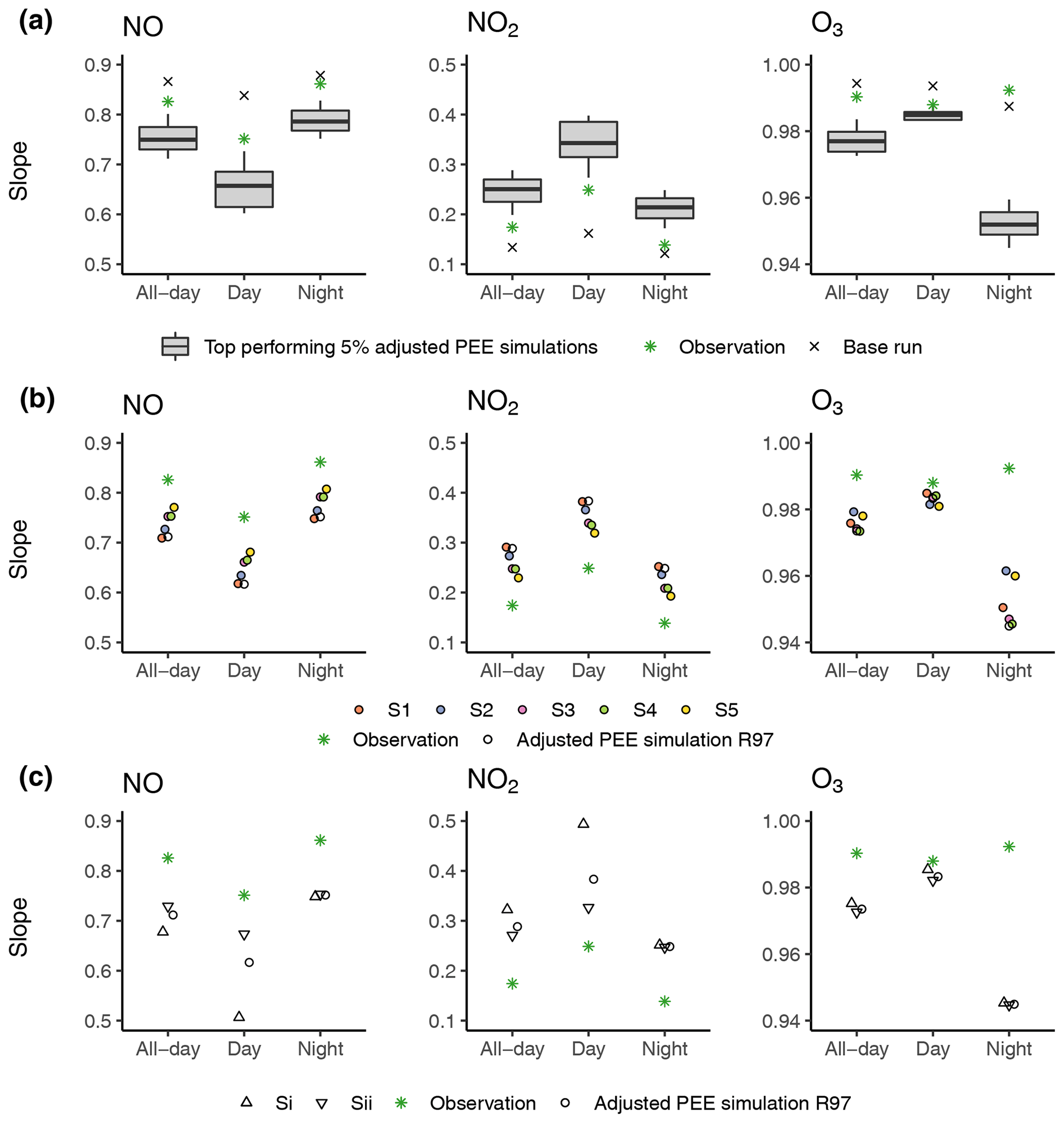
Figure 8 Slopes of linear regression models fitted between the modelled hourly mixing ratios of NO, NO₂, log-transformed O₃ and those of NO_x at all SNAQ sites by (a) the top-performing 5 % of the adjusted perturbed emissions ensemble simulations (PEE) and the base run, (b) the background concentration sensitivity simulations and the best PEE simulation R97, (c) the ROC concentration sensitivity simulations and the best PEE simulation R97, compared to the corresponding slopes fitted to SNAQ measurements. The slopes for log-transformed O₃ as a function of NO_x are exponentiated. Details of the background concentration sensitivity simulations are provided in Table S3. The simulations Si and Sii represent a doubling and halving of the ROC concentrations (by modifying the reactivity coefficient) in R97, respectively. In all panels, daytime is defined as complete hours between sunrise and sunset in Beijing during November–December 2016, namely 08:00–15:00 LT.

We then fitted linear models to the corresponding output (i.e. for the same locations and time frame) from the top-performing 5 % of the adjusted PEE simulations (see Sect. 3). These are compared with models fitted to the SNAQ measurements with respect to the slope, as it indicates the number of changes in NO, NO₂ and (log-transformed) O₃ as NO_x increases/decreases, which is directly related to the input NO_x emissions. As can been seen from Fig. 8a, the modelled slopes of the linear models between NO₂ and NO_x are higher, whereas modelled slopes for NO as a function of NO_x are lower compared to those observed, irrespective of the time of day. The discrepancies between modelled and observed slopes for O₃ as a function of NO_x are relatively small. This suggests that with similar concentrations of NO_x as observed, the top-performing adjusted PEE simulations tend to overestimate NO₂ while underestimating NO. In other words, lower NO_x emissions may be needed for the model to simulate NO₂ concentrations that are consistent with the observations. This suggests that the constrained emission estimates of NO_x are indeed sensitive to the NO_x photolytic chemistry in ADMS-Urban and, in this case, may be low-biased.

There are several possible explanations for the model's tendency to partition more (less) NO_x into NO₂ (NO). As described in Sect. 2.3, the reaction with O₃ (Reaction R4) and reactions with the HO₂ or RO₂ (Reaction R2) are the two pathways of NO oxidation to form NO₂ in ADMS-Urban. Organic radicals are produced via Reaction (R1) in which ROC is defined as the proportion of TVOC that is reactive and calculated by multiplying the TVOC concentrations with a reactivity coefficient. In ADMS-Urban version 4.2 (used in this study), a coefficient of 0.1 is adopted. It is set to 0.05 in the most up-to-date version 5 (Cambridge Environmental Research Consults Limited, 2017, 2020). As a secondary pollutant, modelled O₃ concentrations depend on the input background levels, for which there is no widely accepted definition. To investigate the sensitivity of the model output to these two NO oxidation pathways, a series of sensitivity simulations were performed. All simulations were input with the same NO_x (and VOC) emissions as R97, the adjusted PEE simulation with the best performance in simulating hourly NO₂ concentrations at the long-term monitoring sites. Again, simple linear regression models were fitted between hourly mixing ratios of NO, NO₂, (log-transformed) O₃ and NO_x output by these simulations.

Figure 8b shows that different definitions of background NO₂ and/or O₃ (see Table S3) indeed have an impact on the modelled NO-to-NO₂ conversion. For example, in the sensitivity simulation S5 input with the lowest background levels of NO₂ and O₃, the modelled slopes for NO₂ as a function of NO_x are considerably lower than the corresponding slopes modelled by R97 and thus closer to the observed slopes. Also, the slopes between NO and NO_x associated with outputs from S5 are higher than those found in outputs from R97 and agree better with the observed slopes. However, it is important to underscore that this does not suggest that the 10th percentile concentration is most representative of the background concentrations of NO₂ and O₃. It simply highlights the impact of the input background concentrations of reactive pollutants on the model outputs of relevant species (and thus on the emission estimates inferred on the basis of these model outputs), which can be comparable to the impact of varying the input NO_x emissions (amongst the top-performing 5 % of the adjusted PEE simulations) shown in Fig. 8a. This calls for further research into appropriate definitions for background levels of NO_x and O₃ within a vast and heterogeneous urban area like the modelling domain in this study. Also, it is worth noting that the modelled chemistry is also influenced by the input background levels of NO. However, the specific sensitivities were not investigated, as the upwind concentrations extracted from the CAMS reanalysis dataset are the only set of NO observations available long-term.

The effect of organic radicals on the partition of NO_x between NO₂ and NO is shown in Fig. 8c by varying the concentrations of ROC. As explained above, ROC concentrations are controlled by both the TVOC concentrations (that result from the input emissions and background levels of VOC) and a reactivity coefficient which was set to 0.1 in R97 (as with other adjusted PEE simulations). With fixed TVOC concentrations, using a coefficient of 0.2 doubles the ROC available to produce HO₂ and RO₂, leading to an even more pronounced overestimation of NO₂, accompanied by an underestimation of NO. In contrast, halving the ROC concentrations by using a coefficient of 0.05 partitions less of the NO_x emitted into NO₂. This highlights that the emissions and background concentrations of VOC (which are not evaluated in this study due to a lack of observations) also have an impact on the modelled NO_x photolytic chemistry and thus the a posteriori emission estimates of NO_x. It is also worth noting that biogenic VOCs are likely underestimated in the current simulations, as these are only represented by one of the eight species (i.e. isoprene) output by the CAMS reanalysis product used to approximate the background levels of TVOC and are not represented at all in the base emissions (which include anthropogenic sources only). Despite having low concentrations in the study area (compared to anthropogenic VOCs) (Mo et al., 2018), they are associated with high radical production and thus O₃ creation potentials. Unlike background concentrations of NO_x and O₃, however, the effect of VOCs on the modelled NO_x–O₃ chemistry is restricted to daylight hours, as they only produce radicals in the presence of solar radiation in the model.

Another factor that affects the modelled NO_x photolytic chemistry is the f-NO₂ in the input emissions (see Sect. 3.1). Although not investigated with sensitivity experiments, it can be expected that a higher f-NO₂ would result in higher NO₂ concentrations and lower NO concentrations simulated by the model, thus further increasing the discrepancies between the modelled and observed slopes of linear functions, whilst a lower f-NO₂ would have the opposite effect.

5 Conclusions

We developed a novel approach to update a priori emission estimates using ground-based network measurements as constraints and an ensemble of forward simulations which are input with a PEE. Using this approach, we were able to update the transport sector NO_x emissions in Beijing from a 2013 emissions inventory for the year 2016. The updated emissions are substantially lower with a higher proportion occurring at night-time and are broadly consistent with findings of several previous studies. It would be possible to also update emissions from other (non-negligible) source sectors, provided that appropriate measurements were available.

As with existing emission optimisation techniques, this approach is sensitive to the chemical mechanisms in the underlying model, the uncertainties of which can be propagated into uncertainties in the emission estimates. Nonetheless, this approach has several unique advantages. Compared to inverse modelling techniques, the construction of a PEE and the forward simulations is rapidly executable. Even when the Gaussian dispersion model used in this study is replaced with a CTM for more explicit representations of chemistry, the efficiency can be maintained via parallel computing. Also, surface-based measurements of ambient concentrations are used as constraints, which are readily available and closer to the sources of emissions than the satellite-based measurements. This proximity to emission sources may be particularly important for capturing the high temporal and spatial variability of highly reactive species. For example, Qu et al. (2021) found that in comparison to surface concentrations, the NO₂ column showed a muted response to the step decrease in NO_x emissions in the United States during the COVID-19 crisis. Most importantly, this approach allows for an update of emissions by source sector, which is more relevant for policy interventions than total emissions, as they directly reflect the (in)effectiveness of the corresponding pollution control measures. Hence, we believe that this approach, particularly combined with low-cost sensors, has great potential in providing timely updates of emissions in regions undergoing rapid changes, where emissions inventories may be biased or outdated as soon as they have been compiled, and computing facilities may be limited.