the Creative Commons Attribution 4.0 License.
the Creative Commons Attribution 4.0 License.
 | 05 Jul 2022
Quantifying the impact of meteorological uncertainty on emission estimates and the risk to aviation using source inversion for the Raikoke 2019 eruption
Natalie J. Harvey
Helen F. Dacre
Cameron Saint
Andrew T. Prata
Helen N. Webster
Roy G. Grainger
Due to the remote location of many volcanoes, there is substantial uncertainty about the timing, amount and vertical distribution of volcanic ash released when they erupt. One approach to determine these properties is to combine prior estimates with satellite retrievals and simulations from atmospheric dispersion models to create posterior emission estimates, constrained by both the observations and the prior estimates, using a technique known as source inversion. However, the results are dependent not only on the accuracy of the prior assumptions, the atmospheric dispersion model and the observations used, but also on the accuracy of the meteorological data used in the dispersion simulations. In this study, we advance the source inversion approach by using an ensemble of meteorological data from the Met Office Global and Regional Ensemble Prediction System to represent the uncertainty in the meteorological data and apply it to the 2019 eruption of Raikoke. Retrievals from the Himawari-8 satellite are combined with NAME dispersion model simulations to create posterior emission estimates. The use of ensemble meteorology provides confidence in the posterior emission estimates and associated dispersion simulations that are used to produce ash forecasts. Prior mean estimates of fine volcanic ash emissions for the Raikoke eruption based on plume height observations are more than 15 times higher than any of the mean posterior ensemble estimates. In addition, the posterior estimates have a different vertical distribution, with 27 %–44 % of ash being emitted into the stratosphere compared to 8 % in the mean prior estimate. This has consequences for the long-range transport of ash, as deposition to the surface from this region of the atmosphere happens over long timescales. The posterior ensemble spread represents uncertainty in the inversion estimate of the ash emissions. For the first 48 h following the eruption, the prior ash column loadings lie outside an estimate of the error associated with a set of independent satellite retrievals, whereas the posterior ensemble column loadings do not. Applying a risk-based methodology to an ensemble of dispersion simulations using the posterior emissions shows that the area deemed to be of the highest risk to aviation, based on the fraction of ensemble members exceeding predefined ash concentration thresholds, is reduced by 49 %. This is compared to estimates using an ensemble of dispersion simulations using the prior emissions with ensemble meteorology. If source inversion had been used following the eruption of Raikoke, it would have had the potential to significantly reduce disruptions to aviation operations. The posterior inversion emission estimates are also sensitive to uncertainty in other eruption source parameters and internal dispersion model parameters. Extending the ensemble inversion methodology to account for uncertainty in these parameters would give a more complete picture of the emission uncertainty, further increasing confidence in these estimates.
- Article
(3474 KB) - Full-text XML
- BibTeX
- EndNote


Volcanic ash poses a significant risk to aviation as it can cause engines to malfunction and block the system that monitors air speed, and external corrosion can reduce visibility (Casadevall, 1994; Clarkson et al., 2016; Clarkson and Simpson, 2017). In the event of a volcanic eruption, authorities need to make fast decisions about which routes are safe to operate and ensure that airborne aircraft land safely. Safety is of paramount importance, but the grounding and re-routing of aircraft come with a large economic cost (e.g. it is estimated that the 2010 eruption of the Icelandic volcano Eyjafjallajökull cost the airline industry over GBP 1 billion, Mazzocchi et al., 2010). Further costs are incurred through the increased maintenance and checks that need to be performed if an aircraft is deemed to have potentially encountered ash. The aim of this paper is to demonstrate the usefulness of applying an inversion technique that optimally combines satellite retrievals and ensemble dispersion simulations to provide an ensemble of the most probable source emission estimates of volcanic ash that will undergo long-range transport. Here, the technique is applied to the 2019 Raikoke eruption. This volcano is in a very remote location with no co-located ground-based remote sensing that can be used to determine the height of the eruption plume. Also, at the time of the eruption, the meteorological situation was rapidly evolving with a large cyclone developing in the North Pacific, resulting in the complex filamentation of the volcanic ash cloud. The application of the ensemble inversion approach to this case study demonstrates the benefits of representing the uncertainty in the meteorological data. The results quantify confidence in both the emission estimates and associated ash forecasts.
Currently, the short-range forecast of the geographical location of ash is disseminated to the aviation sector by Volcanic Ash Advisory centres (VAACs), using Volcanic Ash Advisories (VAAs) and Volcanic Ash Graphics (VAGs). These advisories are a combination of output from a Volcanic Ash Transport and Dispersion Model (VATDM), observations of the ash cloud (both from satellites and the ground), pilot reports and forecaster judgement. They indicate the expected location of the ash cloud, but contain no quantitative information about ash concentration. Following the 2010 Eyjafjallajökull eruption, the UK Met Office (home of the London VAAC) also began producing quantitative peak concentration forecasts for North Atlantic and European areas. These forecasts use three concentration thresholds that define the following levels of ash contamination: low (200–2000 µg m−3), medium (2000–4000 µg m−3) and high (> 4000 µg m−3) (UK Civil Aviation Authority, 2017). These thresholds were determined through consultation between the United Kingdom’s Civil Aviation Authority (CAA), Rolls-Royce plc, the UK Met Office, international and European regulators, and aviation experts (Witham et al., 2012; Clarkson et al., 2016). Aviation operators are required to have a safety risk assessment approved by their national aviation authority before aircraft are permitted to fly in regions of medium and high ash contamination (European Commission, 2011; UK Civil Aviation Authority, 2017). The Roadmap for International Airways Volcano Watch (IAVW) in Support of International Air Navigation (Meteorology Panel International Civil Aviation Organization, 2019) state that from 2025, not only will quantitative ash forecasts need to be provided, but also uncertainty information, potentially through the use of ensembles of VATDM simulations.
The forecasting of ash location and concentration following an eruption is strongly dependent on information about the eruption that is used to initialise the VATDM simulations (e.g. Webley et al., 2009; Dacre et al., 2011; Stohl et al., 2011; Tesche et al., 2012; Webster et al., 2012; Harvey et al., 2018; Prata et al., 2019). Typically, VATDMs require that the eruption location, start time, duration, particle size distribution and ash density be specified. Plus, the time evolution of the height of the ash plume, the vertical distribution of the ash within the eruption column and the mass eruption rate also need to be defined. It is possible to estimate the eruption start time using satellites or local observers. There are several remote sensing techniques to estimate the height of the ash plume (e.g. Oppenheimer, 1998; Petersen et al., 2012). Mass eruption rates are typically estimated using empirical relationships based on the reported plume height and ash deposits from past eruptions (e.g. Mastin et al., 2009; Sparks et al., 1997). However, these empirical relationships do not account for other factors that may influence the plume height, such as the impact of the meteorological situation (e.g. wind-bent plumes (Woodhouse et al., 2013)). This lack of representation of important physical processes and reliance on information from past eruptions can lead to large uncertainties in the erupted mass estimates. By default, the London VAAC assume that volcanic ash has a density of 2300 kg m−3 and a particle size distribution based on data from Hobbs et al. (1991). Recent studies by Bruckert et al. (2021) and Plu et al. (2021) have investigated coupling the detailed plume model FPlume (Folch et al., 2016) to full atmospheric modelling systems, ICON-ART (ICOsahedral Nonhydrostatic – Aerosols and Reactive Trace gases) and MOCAGE (MOdele de Chimie Atmospherique de Grande Echelle), respectively, to determine the impact of a more realistic description of the emissions from the volcano on the evolution of the simulated ash and sulfur dioxide plume. In both cases, the coupling resulted in a more realistic representation of the emissions and therefore, the horizontal dispersion of the ash plume and a significantly improved ash forecast.
Meteorological forecast information from numerical weather prediction models is also used as input to VATDMs. This information includes time-evolving three-dimensional wind fields, precipitation and meteorological cloud location. These meteorological forecasts inform both the transport and dispersion of the ash cloud and the removal of ash from the atmosphere via wet and dry deposition. The effect of turbulence and small-scale atmospheric motions, which are not resolved in the input meteorology, are parameterised within the VATDM. Currently, operational VATDMs do not typically consider uncertainties in the meteorological situation as they only use one realisation of the meteorological forecast. These uncertainties can potentially lead to significant errors in the forecast ash cloud position and concentration. These errors often occur where ash particles encounter regions of large horizontal flow separation in the atmosphere. Ash particle trajectories that originate from very similar locations can diverge quickly, leading to a reduction in the accuracy of the deterministic forecast (Dacre and Harvey, 2018). One method of representing this uncertainty is to use an ensemble of meteorological forecasts as input for VATD models. This approach has been advocated by the volcanic ash community for some time as a way to account for wind and precipitation uncertainty (Bonadonna et al., 2012). However, ensemble meteorology is not routinely used operationally at the VAACs. This is due to several different barriers, including the requirement for VAAs and VAGs to be issued within a prescribed time window and the need to present the ensemble forecasts in a format that can be used by decision makers to make fast and robust decisions in an emergency response situation (Mulder et al., 2017).
The use of ensemble meteorology to produce an ensemble of dispersion simulations as a research tool is not new (e.g. Straume et al., 1998; Galmarini et al., 2004, 2010), but there are only a small number of studies that apply this approach to volcanic ash forecasts. Recent work by Zidikheri et al. (2018) found that using an ensemble of dispersion model simulations driven by an ensemble of meteorological fields and different values of ash source parameters gave increased skill at all lead times (the length of time between when the forecast is issued and the time the phenomena are predicted to occur), compared to a deterministic forecast. A study focussing on the 2013 eruption of Kelut (Dare et al., 2016) found that if an ensemble is used, rather than a single realisation of the meteorological situation, there are better qualitative agreements with satellite observations for lead times greater than 12 h and similar agreements with satellite observations at lead times shorter than 12 h. This is relevant for the VAAs and VAGs as they are issued out to a forecast lead time of 18 h. Two earlier studies by Stefanescu et al. (2014) and Madankan et al. (2014) found that there can be a large spread in predicted ash concentrations at lead times greater than 48 h when using ensemble meteorology. These studies suggest that the use of ensembles can provide useful additional volcanic ash forecast information. However, there is a need to develop strategies to extract information from them that are useful for decision-making at longer lead times.
Satellite imagery in the visible and infrared can show the presence and extent of volcanic ash clouds. Advances in satellite retrieval techniques mean that estimates of ash cloud top height, effective ash radius and ash column loading are also available (e.g. Francis et al., 2012; Pavolonis et al., 2013; Grainger et al., 2013). Mass eruption rates at the neutral buoyancy level can be estimated under certain assumptions (e.g. Woods and Kienle, 1994; Pouget et al., 2013; Prata et al., 2021a), but direct retrievals of the vertical distribution within the eruption column are not possible. However, satellite retrievals, typically of ash column loading, can be combined with VATDM simulations using inversion techniques to give time-evolving estimates of these crucial quantities. There are numerous published approaches that use inversion modelling to estimate ash source parameters for volcanic eruptions (e.g. Kristiansen et al., 2012; Schmehl et al., 2012; Denlinger et al., 2012; Pelley et al., 2021; Zidikheri et al., 2017a, b), using a single deterministic realisation of the meteorological situation. This means that uncertainty in the forecast precipitation or three-dimensional wind fields will lead to uncertainty in the estimated mass eruption rates and their vertical distribution.
As in Harvey et al. (2020), this study brings together inverse modelling and the use of an ensemble of meteorological forecasts to give an ensemble of the most probable source emission estimates of volcanic ash that will undergo long-range transport following the 2019 Raikoke eruption. These emission estimates can be used to obtain robust ash forecasts constrained by observations. There will be a particular focus on regions where medium and high levels of ash contamination are predicted, as these are areas where aircraft may be prohibited from entering. There will also be a focus on the influence of emissions of ash into the stratosphere on these regions.
The methods and data used in this study are described in Sect. 2. Section 3 describes the details of the 2019 Raikoke eruption. The volcanic emission estimates determined using the ensemble inversion system, their impact on volcanic ash forecasts and their impact on flight planning decisions are presented in Sects. 4 and 5. A summary, conclusions and implications for future work are presented in Sect. 6.
2.1 NAME
In this study, the Numerical Atmospheric-dispersion Modelling Environment (NAME) model was used to simulate the dispersion of volcanic ash (Jones et al., 2007). To model the transport and removal of volcanic ash, NAME includes parameterisations of dispersion due to free tropospheric turbulence (Webster et al., 2018), sedimentation and dry deposition (Webster and Thomson, 2011), and wet deposition (Webster and Thomson, 2017). It is assumed that the ash particles are spherical and have a density of 2300 kg m−3 (Bonadonna and Phillips, 2003), but, in reality, the density of the ash is determined by its porosity, chemical composition and grain size. In this study, aggregation of ash particles, near-source plume rise and processes driven by the eruption dynamics (e.g. Woodhouse et al., 2013) are not explicitly modelled. The particle–size distribution used is based on data from Hobbs et al. (1991), but only includes ash particles with diameters between 1–30 µm, as ash particles larger than this are not typically detected by the Advanced Himawari Imager (AHI). We refer to this as fine ash in this paper. Three NAME simulations were performed using nominal emissions, prior emissions and posterior emissions (Fig. 1).
2.2 Ensemble of meteorological forecasts
The Met Office Global and Regional Ensemble Prediction System (MOGREPS-G) has 17 ensemble members plus a control member (Bowler et al., 2008). It has a horizontal resolution of 20 km in mid-latitudes, and there are 70 vertical levels with the lid at approximately 80 km. Each forecast is initialised four times per day at 00:00, 06:00, 12:00 and 18:00 UTC and they extend out for 7 d. At the time of the Raikoke eruption, MOGREPS-G used a stochastic physics scheme to account for model uncertainty and an online inflation factor calculation to calibrate the spread of the ensemble in space and time (Flowerdew and Bowler, 2011, 2013). The horizontal resolution of the deterministic global configuration of the Met Office Unified Model is currently around 10 km in the midlatitudes. This is higher than the horizontal resolution of the MOGREPS-G ensembles used in this study. The disadvantage of using lower-resolution meteorology is that it may result in less accurate dispersion simulations, as mesoscale features in the atmosphere cannot be resolved. However, the advantage is that ensembles are inherently probabilistic, so we can express the uncertainty directly. Furthermore, it has been shown that ensembles of lower-resolution models can provide greater skill than single forecasts of higher-resolution models (e.g. Grimit and Mass, 2002). The MOGREPS-G forecasts used to drive NAME in this study are initialised at 12:00 UTC 21 June 2019 and are of 78 h in duration (Fig. 1).
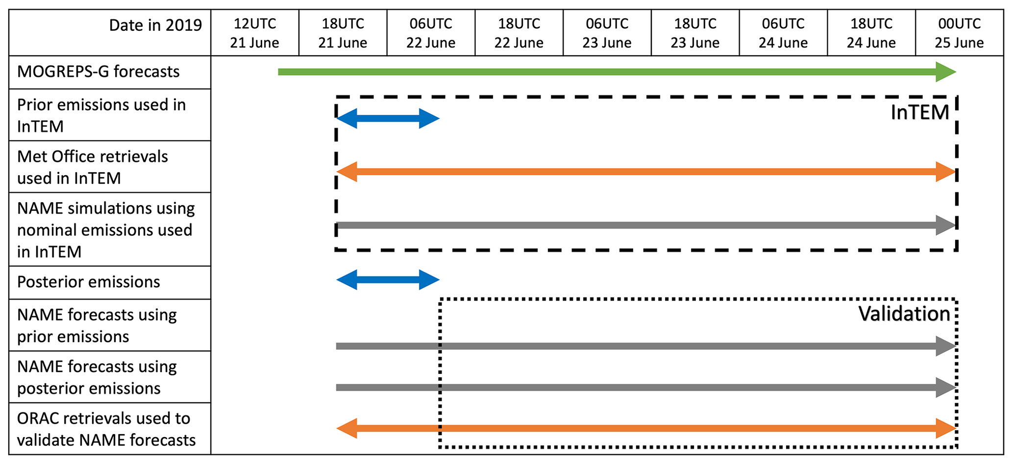
Figure 1Timeline showing start and end of volcanic emissions used in the NAME simulations (blue arrows), satellite retrievals used for source inversion and validation (orange arrows), meteorological forecast data period (green arrow) and NAME simulation length (grey arrows). Single-headed arrows represent forecasts and double-headed arrows represent volcanic ash emission and observation data periods. The dashed box surrounds data sources used in the InTEM source inversion and the dotted box surrounds data used in the validation.
2.3 Satellite observations
In this study, two different volcanic ash retrievals are used (Fig. 1). They are both based on Himawari-8 satellite measurements. The Met Office retrieval is used for the source inversion described in section 4.1, and the ORAC retrieval is used to evaluate the sensitivity of the inversion to the satellite retrieval algorithm and for semi-independent validation of the inversion results described in Sect. 4.2.
2.3.1 Himawari-8
Himawari-8 is a geostationary satellite with 16 spectral channels that came into operation in July 2015 (Bessho et al., 2016). Its high temporal (10 min) and spatial (2 km at nadir for the infrared bands) resolution make its observations ideally suited to evaluate the transport of volcanic ash following an eruption. Two volcanic ash retrieval algorithms, one based on work primarily from the UK Met Office (Francis et al., 2012) and one determined using the methodology described in McGarragh et al. (2018) are used in this study and described below. Note that although the retrieval methods have been developed independently in different research groups, they both use information from the Himawari-8 satellite and therefore have the same bias when volcanic ash is obscured by a meteorological cloud (which was prevalent during the Raikoke 2019 eruption). The purpose of using two retrieval algorithms is to determine if our conclusions are sensitive to the choice of satellite retrieval.
2.3.2 Met Office algorithm
This algorithm is based on the method described in Francis et al. (2012) and uses a reverse absorption technique with slight adaptations for the channels of the AHI. Firstly, the channels at 8.6, 10.4 and 12.4 µm are used to differentiate between meteorological and ash clouds. Then the ash column loading, layer height and effective radius are determined using a one-dimensional variational (1D-Var) analysis to determine an optimal estimate between the assumed background and the observed radiances in the channels at 10.4, 12.4, and 13.3 µm. The detection is based on a combination of brightness temperature difference (BTD) tests and beta ratio tests that are optimised for the 25 June 2019 Raikoke eruption. The beta ratio tests use a derived radiative parameter β, originally devised by Pavolonis (2010). The beta ratios (the effective absorption optical-depth ratio of two channels) are calculated for both the 12.4, 10.4 µm combination and the 8.6, 10.4 µm combination. Both β (12.4, 10.4) and β (8.6, 10.4) are used to filter pixels detected by the BTD tests. To reduce false detections over arid land surfaces and at a high satellite zenith angle, several geographical filters are used. Checking the consistency of ash detection in neighbouring pixels also removes other false detections. The detection limit for thermal infrared retrievals is 0.2 g m−2 (Prata and Prata, 2012).
Meteorological data from the Met Office Unified Model are used in both the detection and retrieval algorithms. In the detection algorithm, meteorological data are required to calculate clear sky and overcast radiances (Francis et al., 2012). These are then used to derive the emissivities used to calculate the beta ratios. Similarly, the retrieval algorithm uses the clear sky and overcast radiances as part of the radiative transfer model.
Where ash is detected, the Met Office algorithm determines the ash column loading. These pixels are flagged as containing ash. If a pixel is free from both ash and meteorological cloud, then it is flagged as a clear-sky pixel. Pixels that do not have detectable ash and are not flagged as clear skies (i.e. they may contain meteorological cloud) are unclassified. As in Pelley et al. (2021), further processing is performed to re-grid the retrieved column loadings onto a grid of 0.375∘ latitude by 0.5625∘ longitude (approximately 40 km × 40 km in mid-latitudes) and averaged over 1 h. This is to match the resolution of the NAME ash column loading output and reduce data volumes. Following the study by Pelley et al. (2021), we use thresholds to account for representativity errors within a grid box. If 50 % or more satellite pixels in a grid box contain ash or more than 90 % of pixels are classified as ash or clear skies, then the grid box is selected for use in the InTEM (Inversion Technique for Emission modelling). If all classified pixels within a grid box are flagged as clear sky pixels, then the grid box is deemed to be a clear sky observation. Otherwise, the grid box is deemed to be an ash grid observation with the column loading in this grid box given by the mean of all the classified pixels (including clear skies).
2.3.3 ORAC algorithm
To estimate the mass loading of ash for the Raikoke ash clouds, the Optimal Retrieval of Aerosol and Cloud (ORAC, McGarragh et al., 2018) algorithm was applied to infrared measurements made by the AHI on board the Himawari-8 satellite. ORAC uses the optimal estimation approach (Rodgers, 2000) to retrieve state variables based on radiative transfer simulations, satellite measurements and prior information. The ORAC retrievals use ECMWF Reanalysis (ERA5) meteorological data to model the radiative transfer that is affected by temperature, specific humidity and trace gas profiles. The ORAC algorithm includes optical depth, effective radius, surface temperature and cloud-top pressure in the state vector, and the mass loading is derived from the retrieved optical depth and effective radius, consistent with previous authors (e.g. Wen and Rose, 1994; Corradini et al., 2008; Prata and Prata, 2012). The 10.4, 11.2, 12.4 and 13.3 µm thermal infrared channels are used in the measurement vector. The microphysical model used in the radiative transfer model assumes an ash cloud contains spherical particles, which conform to a log-normal distribution and ash composition based on the Eyjafjallajökull ash taken from the Aerosol Refractive Index Archive (ARIA, https://eodg.atm.ox.ac.uk/ARIA/, last access: 25 November 2021). Ash detection follows the approach presented in Appendix A of Prata et al. (2021b), and only retrievals that converge with a measurement cost at a solution of less than 10 are considered (Thomas and Siddans, 2015). For the Raikoke case, we found that false detections (isolated pixels unrelated to the main volcanic plume/cloud) often had cost values higher than 10. Setting a cost threshold of 10 therefore provided a good balance between false positives and true positives. Four forward model configurations are used in the retrievals: (1) a single tropospheric layer of ash, (2) a tropospheric ash layer above a liquid water cloud layer, (3) a single stratospheric layer of ash, and (4) a stratospheric ash layer above a liquid water cloud layer. The multi-layer configurations are introduced to account for prevalent low-level stratus clouds during the explosive phase of the Raikoke eruption. The water cloud layer is tightly constrained with an a priori cloud-top pressure of 800 hPa, effective radius of 10 µm and 550 nm optical depth of 16. The a priori uncertainties on these values are set to 50 hPa, 1 µm and 3. The a priori settings were chosen based on ORAC standard cloud retrievals (Poulsen et al., 2012; McGarragh et al., 2018) that are run separately on nearby, low-level stratus clouds.
The troposphere/stratosphere model configurations are run by setting two different a priori cloud-top pressures to determine cloud-top heights above and below the tropopause. The a priori cloud-top pressures considered are 500 and 200 hPa. The stratospheric a priori cloud-top pressure is chosen based on independent CALIPSO observations of the stratospheric ash cloud. After running all four forward model configurations, we select the retrieval with the lowest cost for each ash-affected AHI pixel to generate the final retrieval product.
2.4 InTEM for volcanic ash
The Inversion Technique for Emissions Modelling (InTEM) for volcanic ash is an inversion system that combines VATDM simulations, satellite retrievals and a prior estimate of the emission, using a Bayesian approach to give the best estimate of the emissions profile for fine ash that can undergo long-range dispersion (Fig. 1). This system was developed at the UK Met Office and was originally developed to estimate greenhouse gas emissions (Manning et al., 2011). It has been previously used by Harvey et al. (2020) to assess the impact of ensemble meteorology on estimates of volcanic ash emissions from the 2011 Grímsvötn eruption. The posterior emission profile can either be determined using satellite retrievals of ash only or of both ash and clear skies, and has a chosen vertical resolution of 4 km and a time resolution of 3 h. Full details of the InTEM system for volcanic ash are given in Pelley et al. (2021) and Harvey et al. (2020).
2.4.1 Estimate of the prior source term
To ensure that the inverted source term is not over-fitted to the satellite information, a prior estimate of the source term is used. This also ensures that the posterior source term is informed by known information about the eruption, such as the eruption start and end time and the maximum plume height. To construct the prior, it is assumed that emissions in the eruption column are uniform in the vertical from the volcano vent to an estimate of the plume height based on observations with an error of ± 2 km. The mass eruption rate is determined using the empirical relationship in Mastin et al. (2009). The mean and error covariance matrix of the prior are estimated using a stochastic model that includes correlations between errors in the emissions at different heights and times. Thomson et al. (2017) contain a full description of how the prior is determined and used in the InTEM system. In this study, the prior source term is based on a plume height of 13 km, which is consistent with information provided by the Tokyo VAAC and Bruckert et al. (2021), who used a combination of GOES-17 (Geostationary Operational Environment Satellite) data and pilot reports. Note that the prior is a probability distribution and from now on, it is assumed that when the prior is mentioned, it refers to the mean of this distribution.
2.4.2 VATDM simulations
The VATDM simulations within InTEM are performed using NAME. As this methodology exploits ash column loadings determined from satellite retrievals, the NAME simulations only include ash particles with diameters between 1–30 µm, as ash particles larger than this are not typically detected by the AHI. This assumption is consistent with those made in other inversion systems for this application (e.g. Stohl et al., 2011). Simulations representing a nominal release rate (1 g s−1) from each possible source term component (4 km height range and 3-hourly time period) are conducted. Model predictions of ash column loads can be easily determined for a posterior emission profile by a scaled linear combination of these nominal simulations. The resolution of the posterior emission estimate (3-hourly with 4 km vertical resolution) is chosen to ensure that the inversion can be performed within a timeframe that is compatible with VAAC operational constraints.
2.4.3 The inversion algorithm
The prior estimate, NAME simulations and satellite retrievals are combined within the inversion scheme to give a posterior distribution of emissions. The posterior distribution is Gaussian and within InTEM, the best estimate of emissions is taken as the mode of this distribution, with a non-negative constraint applied. It is possible that selecting the mode of the distribution ignores a large amount of uncertain information within the posterior and results in a loss of information about the emissions, but this is not the focus of the present study. A quadratic cost function, representing the simultaneous fit of the VATDM simulations and satellite retrievals, and between the emission estimate and the prior, is minimised using the Lawson and Hanson (1974) non-negative least squares algorithm. Details of the quadratic cost function can be found in Pelley et al. (2021). This algorithm was chosen as it converges in a finite number of iterations and is very fast. In this study, the inversion algorithm took less than 1 min to run for each of the ensemble members, using satellite retrievals from 18:00 UTC on 21 June to 00:00 UTC on 22 June 2019. The speed of the InTEM system is therefore governed by the length of time it takes to perform the VATDM simulations. The best estimate of the emissions determined by InTEM can then be used as the ash emission profile in simulations used to forecast the evolution of the volcanic ash cloud. From now on, it is assumed that when posterior emissions are used, it is the modal value. Pelley et al. (2021) and Thomson et al. (2017) contain a full description of the inversion scheme.
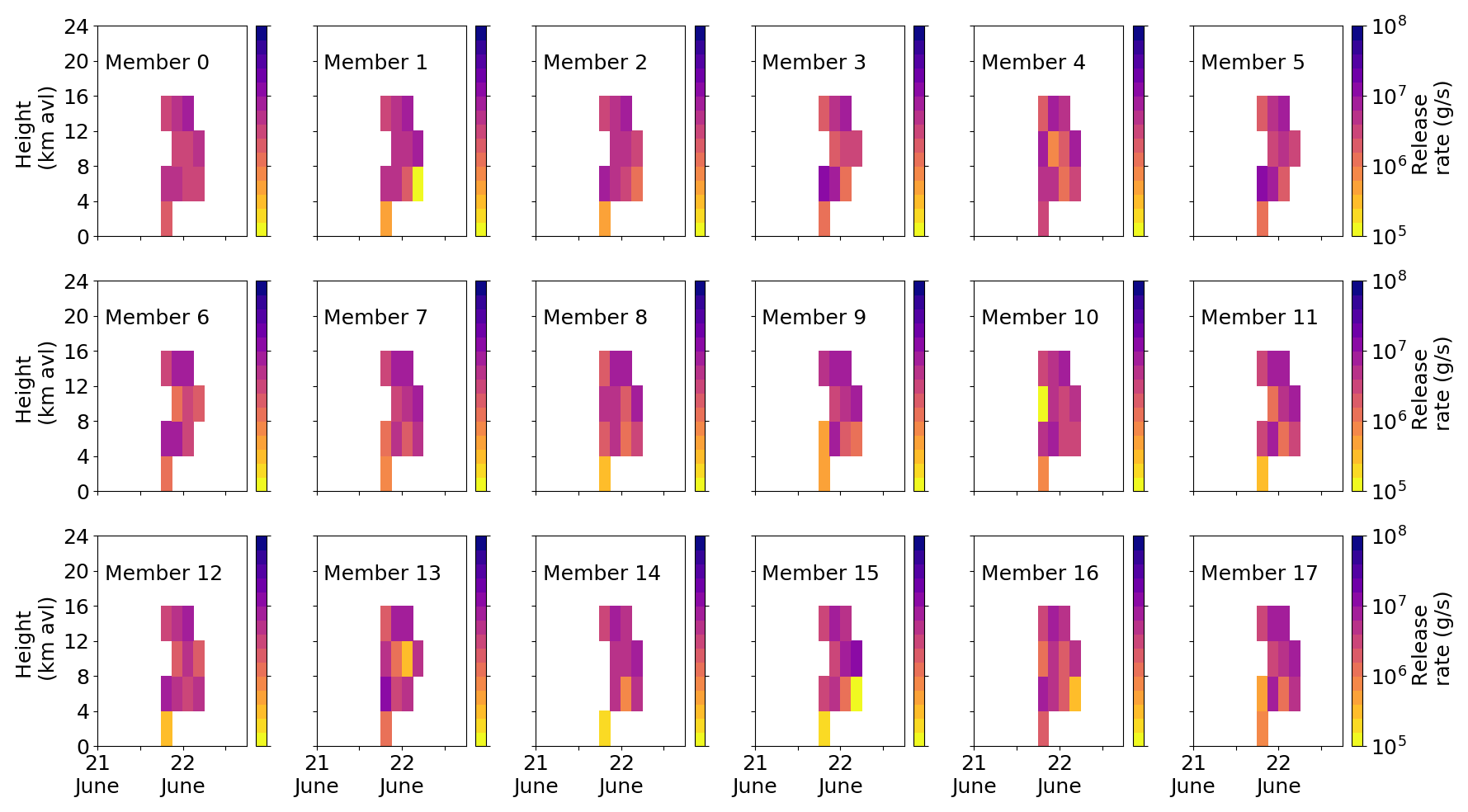
Figure 2Posterior emission profiles (g s−1) estimated by InTEM for the 2019 Raikoke eruption for each member of the MOGREPS-G ensemble, using Himawari retrievals of ash and clear skies. Note the logarithmic colour scale.
Raikoke is an uninhabited volcanic island near the centre of the Kuril Island chain in the Sea of Okhotsk in the northwest Pacific Ocean at 48.2∘ N, 153.3∘ E. The volcano has a vent height of 551 m. Its most recent explosive eruption started at 18:00 UTC on 21 June 2019, when a series of nine explosive events occurred until approximately 06:00 UTC on 22 June. It is estimated that the initial eruptive plume height was 10–14 km a.s.l. (above sea level) (Global Volcanism Program, 2019a), and there is evidence in visible satellite imagery of an umbrella cloud. Ash and sulfur dioxide were dispersed by the jet stream and entrained by a cyclone located near the Komandorskiye Islands. Forty aeroplanes were diverted because of the ash plume produced by this eruption (Global Volcanism Program, 2019b).
4.1 InTEM posterior inversion estimates
Figure 2 shows the posterior height–time ash emission rates for particles in the range between 1–30 µm, obtained using InTEM for the Raikoke eruption (21–22 June 2019) and using each of the MOGREPS-G meteorological ensemble members with Himawari retrievals of ash and clear skies from 21–24 June. Each panel shows the ash emission rates determined by InTEM using a single member of the MOGREPS-G ensemble. The vertical emission profiles are similar, but there are differences in the magnitude of ash emitted. Four members (e.g. member 4) have continuous emissions of ash between 4–12 km above vent level (avl), whereas the other 14 members have times when there are no emissions of ash at this height range. There is very little ash emitted between 0 and 4 km avl in all members, which is qualitatively consistent with the visible satellite imagery indicating an umbrella cloud shape (although it is important to note that the NAME simulations presented here do not represent the radial spreading of an umbrella cloud, which is a source of uncertainty in the determination of the posterior emissions). There is a range in the total emissions of fine ash over the entire eruption of 0.32–0.71 Tg (shown in Fig. 3 as blue circles), with an ensemble mean value of 0.52 Tg. We can compare the ensemble mean value with other estimates of total fine ash estimated from measurements from the Advanced Himawari Imager. Muser et al. (2020) estimate values of 0.4–1.8 Tg and Capponi et al. (2022) estimate an ensemble mean total fine ash of 0.49 Tg. Both of these estimates are quantitatively similar to the mean value of total fine ash estimated from the InTEM ensemble presented here.

Figure 3Total fine ash emitted during the 2019 Raikoke eruption for each member in the MOGREPS-G ensemble determined using InTEM. Blue circles and grey bars indicate the peak in the posterior distribution and range (± one standard deviation) of the total ash emitted. The black dashed line indicates the ensemble mean total fine ash emissions.
However, it is important to note that a deck of stratus clouds was present at low levels (approximately 2 km), potentially leading to an underestimation of the amount of ash present in the lowest part of the atmosphere. The largest number of observations used in the inversion process is 5314 for ensemble member 10, which is 17 % larger than the smallest number used (4459 with ensemble member 7). This is due to the different dispersion patterns for each ensemble member.
Figure 4a shows the prior emission profile, which was determined using the empirical Mastin relationship (Mastin et al., 2009), and a plume height of 13 km avl, which is consistent with reports from the Tokyo VAAC and the plume heights used in Bruckert et al. (2021). The emission profile is regridded onto the height–time grid used in the inversion; hence, emissions between 12–13 km avl are spread out between 12–16 km. The emission rates are greater at all heights and times when compared to the posterior estimates. The prior total emission is 11 Tg, which is approximately 15.5 times larger than any of the posterior estimates (shown in Fig. 3). Figure 4b shows the ensemble mean posterior emission profile, showing a large reduction in emissions at all levels, especially below 4 km avl where ash is only emitted for one 3 h period at the start of the eruption. This reduction greatly impacts the fraction of emissions released near the surface (0–4 km), in the troposphere (4–12 km) and in the stratosphere (above 12 km), as seen in Fig. 5. Note that the heights chosen here to define the vertical levels in the atmosphere are based on the vertical resolution of the InTEM emission profile. The prior emission profile has 31 % of the ash emitted near the surface, 61 % in the troposphere and 8 % in the stratosphere, compared to the posterior ensemble mean of 3 % of ash emitted near the surface, 63 % in the troposphere and 34 % in the stratosphere. Fractionally, there is a much larger amount of ash emitted into the lower stratosphere in the posterior ensemble. This has consequences for the temporal evolution of the simulated ash cloud, as ash in the stratosphere cannot be easily deposited to the surface through wet deposition and sedimentation. Plus, due to vertical wind shear, ash within the stratosphere can be transported by atmospheric winds with different speeds and directions compared to lower regions of the atmosphere. Simulations of the evolution of the Northern Hemisphere mean sulfur dioxide mass burden from the Raikoke eruption, performed by de Leeuw et al. (2020), were also found to be sensitive to the amount of sulfur dioxide emitted in the stratosphere. The NAME simulation with the best agreement with satellite retrievals of sulfur dioxide from TROPOMI in terms of peak concentrations and e-folding times had a larger fraction of sulfur dioxide emitted in the lower stratosphere compared to the control simulation.
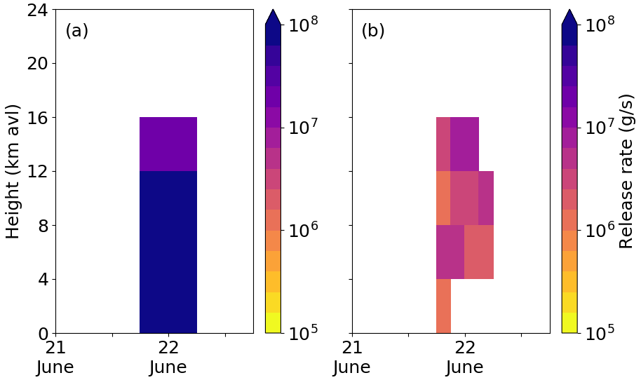
Figure 4(a) Prior (b) ensemble mean posterior time–height emission profile (g s−1) determined by InTEM for the Raikoke eruption. Note the log scale used for the release rate.
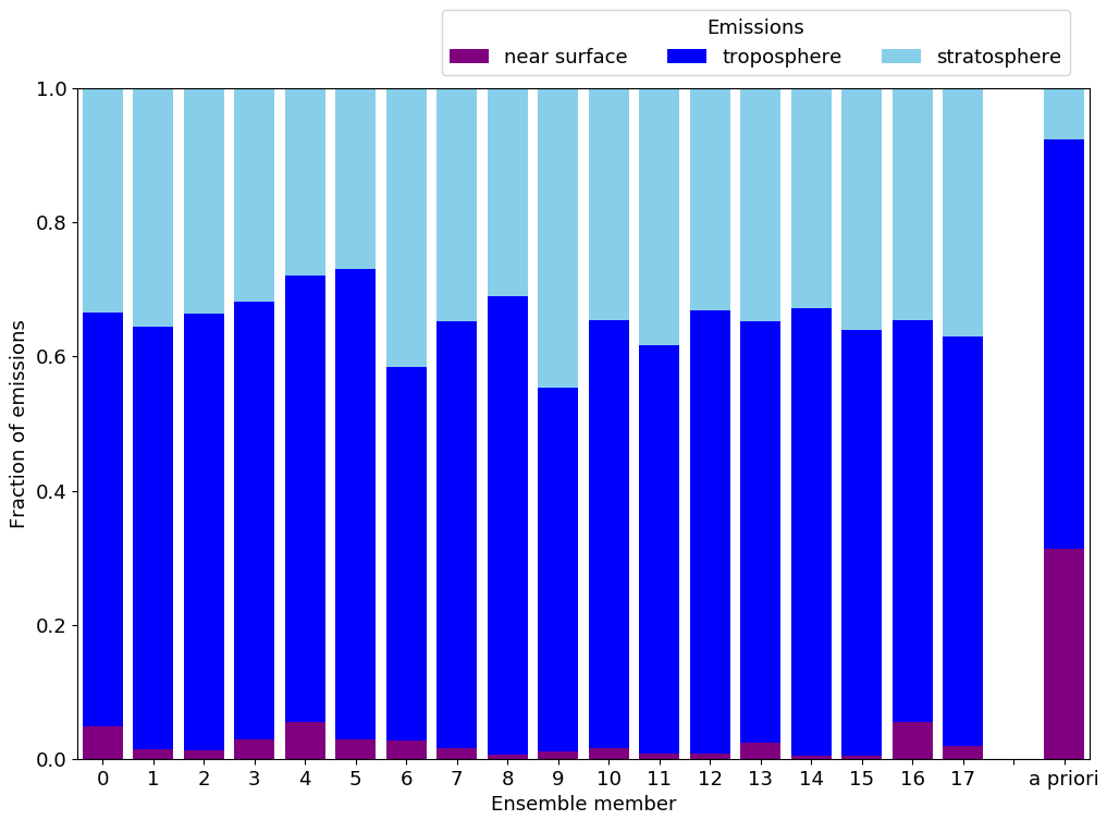
Figure 5The fraction of total ash during the 2019 Raikoke eruption emitted near the surface (0–4 km), in the troposphere (4–12 km) and in the stratosphere (above 12 km) for each member in the MOGREPS-G ensemble determined using InTEM. The final bar shows the fraction of ash emitted near the surface, tropopause and stratosphere in the prior emission profile.
4.2 Ensemble ash forecast validation
The previous discussion in Sect. 4.1 focused on the differences in posterior emission profiles however, VATDM forecasts of the ash cloud are used to inform VAAC graphics and advisories. This section analyses NAME simulations driven with the MOGREPS-G meteorological ensemble, both using the peak of the posterior distribution of emissions (shown in Fig. 2) and prior emissions, and evaluates these simulations against satellite retrievals using the ORAC Himawari retrievals. This analysis is performed to determine if the observation constrained by posterior emission estimates results in a more accurate ash forecast than when using the prior emissions evaluated against a semi-independent set of satellite retrievals. Note that the posterior emissions are determined using satellite retrievals for the period of 21–25 June 2019, and not just those retrievals available before 12:00 UTC 22 June 2019 (Fig. 6) and 12:00 UTC 23 June 2019 (Fig. 7).
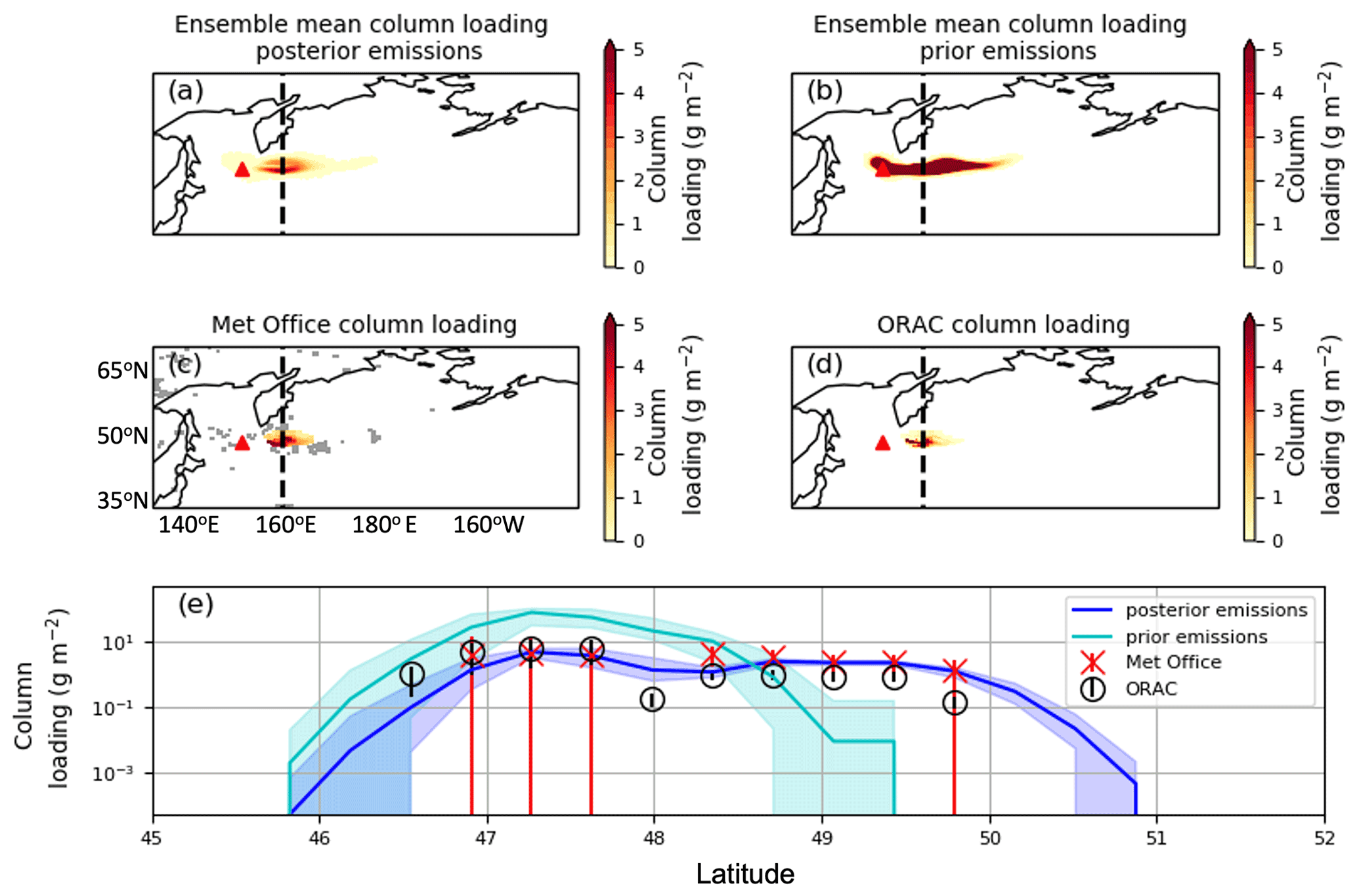
Figure 6(a) Ensemble mean ash column loading for simulations runs with emission profiles determined using InTEM with matching ensemble meteorology at 12:00 UTC 22 June 2019; (b) ensemble mean ash column loading at 12:00 UTC 22 June 2019 for simulations runs with prior emission profile and ensemble meteorology; (c) Himawari ash column loading retrieved using the Met Office algorithm (grey shading indicates grid boxes that are classified as clear sky); (d) Himawari ash column loading retrieved using the ORAC algorithm for 12:00 UTC 22 June 2019; (e) ash column loading profile from 45–52∘ N along the cross section indicated by the black dashed line in panels (a–d). Posterior ensemble (blue), prior ensemble (cyan), Himawari ash column loading retrieved using the Met Office algorithm (red crosses) and Himawari ash column loading retrieved using the ORAC algorithm (black circles). The error bars represent ± 1 standard deviation in the estimates of ash column loading determined from the satellite retrievals. The coloured shading indicates the range of column loading in the ensemble.
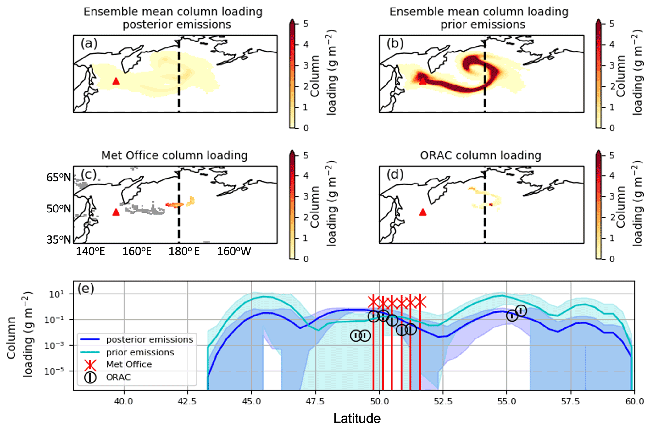
Figure 7As Fig. 6 for 12:00 UTC on 23 June 2019.
Figure 6a–b show the spatial extent of the ash cloud at 12:00 UTC 22 June 2019 for the ensemble of VATDM simulations, with posterior emissions determined using satellite retrievals obtained between 21 and 25 June 2019 (Fig. 6a) and prior emissions (Fig. 6b). Figure 6c–d show Himawari retrievals using the Met Office retrieval algorithm (Fig. 6c) and the ORAC retrieval algorithm (Fig. 6d). There is a large difference between the magnitude of the ash column loadings in the simulated ash clouds in Fig. 6a and b. The mean ash cloud extent from the prior ensemble is similar to the posterior ensemble, but with column loading magnitudes that are more than 10 times larger. In both ensembles, the highest column loadings are in similar locations within the ash plume, with ensemble mean values approximately 68 g m−2 in the prior ensemble and 4.8 g m−2 in the posterior ensemble. By design, the posterior ensemble mean column loading values are quantitatively closer to the satellite retrievals used in the InTEM system (Fig. 6c), but they are also closer to the ORAC retrievals (Fig. 6d) than the prior ensemble mean column loading values.
Figure 7a–b show the ensemble mean column loading using posterior and prior emissions respectively at 12:00 UTC on 23 June 2019. The InTEM-derived posterior estimates use satellite retrievals until 00:00 UTC 25 June 2019. This is 24 h later than the ash cloud shown in Fig. 6. At this time, both the posterior and prior ash clouds are much more extensive than at 12:00 UTC on 25 June 2019, extending as far as 164∘ W. The ash plume is also entrained into a cyclone that was present in the North Pacific at this time. This is most evident in the prior ensemble, where the ensemble mean column loadings are approximately an order of magnitude higher than the posterior ensemble mean column loadings.
Producing an ensemble of VATDM simulations allows the assessment of the ensemble spread. Figure 6e shows the range of posterior column loading values for the 18 posterior emission simulations (blue line and shading) and 18 prior ensemble simulations (cyan line and shading) along the cross section shown in panels (a–d) as a black dashed line. The coloured shading represents the uncertainty in ash column loading due to the meteorological ensemble. Satellite retrievals of ash column loading, and the associated uncertainty from Himawari using the Met Office algorithm (red crosses) and from Himawari using the ORAC algorithm (black circles), are shown for comparison. The Met Office and ORAC retrievals, at this time and along this cross section, are very similar. Between 45–50∘ N, the posterior ensemble spread encompasses the Met Office retrievals within their retrieval uncertainty. Between 46.5–47.6∘ N and 48.4–48.7∘ N, the posterior ensemble spread falls within the uncertainty of the ORAC retrievals. The prior ensemble has a much higher ensemble mean ash column loading than the posterior ensemble (by over a factor of 10), and the ensemble spread does not encompass either set of satellite retrievals within 1 standard deviation. Meteorological clouds obscure much of the domain, so obtaining a contiguous retrieval of ash and clear sky pixels is not possible at this time.
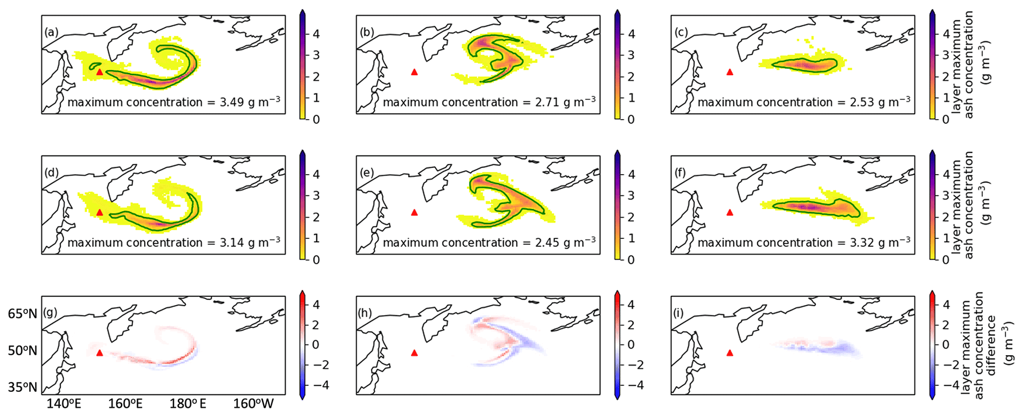
Figure 8Maximum layer ash concentration (g m−3) for (a, d) near surface (0–4 km), (b, e) troposphere (4–12 km) and (c, f) stratosphere (above 12 km), for ensemble member 5 (a–c) and member 9 (d–f) at 12:00 UTC on 23 June 2019. The green contour denotes the 200 µg m−3 concentration level. The lowest ash concentration shown in (a–f) is 100 µg m−3. Panels (g–i) show the difference between maximum layer concentrations for member 5 and member 9, also at 12:00 UTC on 23 June 2019.
Figure 7e shows the same variables as Fig. 6e at 12:00 UTC 23 June 2019. The magnitude of the column loading in the VATDM simulations is approximately 10 % of the column loadings shown in Fig. 6. The prior ensemble column loadings have a large spread in forecast ash column loadings and are indicated by the coloured shading. This spread shows the large variability that can be introduced by using an ensemble of meteorological conditions with the same ash emission profile. In this case, the cross section intersects the simulated ash plume in all of the ensemble members at three locations – 45–46∘ N, 49–51∘ N and 53–59∘ N. However, the Himawari retrievals used in the inversion only detect ash 49–52∘ N. At this location, both the prior and posterior column loadings lie within the uncertainty of the ash retrievals used in the inversion, with the prior emissions lying within 1 standard deviation of the ORAC Himawari ash retrievals. At 55–56∘ N, the posterior ensemble column loadings are within the uncertainty of the ORAC retrievals, but no ash is detected using the Met Office algorithm.
4.3 Vertical distribution of emissions
To assess the impact of a larger fraction of ash being emitted into the stratosphere, we focus on the evolution of the ash plume using inverted emissions and matching meteorology (i.e. the same meteorology is used for both the inversion and the forecast), for ensemble members 5 and 9. These members were chosen as member 5 has the smallest fraction of ash emitted into the stratosphere (27 %), whereas member 9 has the largest (44 %). To determine the differences between the simulations driven by emissions from members 5 and 9, the output from the NAME simulations is post-processed by dividing the vertical grid into three layers (near surface, troposphere and stratosphere), and setting the concentration of each of the three layers to the maximum ash concentration of the original higher resolution layers. Figure 8 shows the maximum of the simulated ash layer concentrations near the surface in the troposphere and stratosphere at 12:00 UTC on 23 June 2019. At this time, a comparison of the different ensemble members shows that the ash plume structure at all three levels is qualitatively very similar. However, there are some differences in plume location, extent and ash concentration values. The location differences are likely due to the use of different driving meteorology. Near the surface and in the troposphere, member 5 has higher maximum concentrations than member 9, but in the stratosphere, the opposite is true. This is expected, as more mass is emitted at these heights in member 9. The differences in peak concentration are largest when considering the stratosphere (2.53 g m−3 in member 5 compared to 3.32 g m−3 in member 9). In the stratosphere, member 9 has the highest peak concentration despite the plume extending further east (by approximately 8∘), the plume having an area 1.4 times larger than the plume produced using member 5, and it being the region with concentrations greater than 200 µg m−3 being 1.5 times larger than the equivalent region in member 5. These differences highlight the importance of the vertical distribution of the ash emissions, as they can lead to an increase in areas that may be considered too contaminated for aircraft to fly through. Note that the lowest ash concentration shown in Fig. 8 is 100 µg m−3.
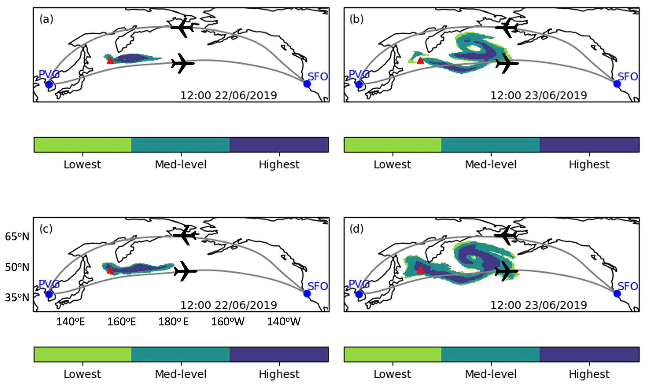
Figure 9Overall ash concentration risk map at (a, c) 12:00 UTC on 25 June 2019, (b, d) 12:00 UTC on 23 June 2019 for (a, b) simulations with posterior emissions with matching ensemble meteorology and (c, d) simulations with prior emissions with ensemble meteorology. Green shading indicates the lowest level of risk, turquoise shading indicates medium-level risk and purple indicates the highest level of risk. The grey line indicates a hypothetical flight route between San Francisco (SFO) and Shanghai (PVG) international airports, with the black aeroplane icons indicating the direction of travel between them.
The comparison between simulated and satellite retrievals of ash column loadings is valuable for forecast validation. However, this variable does not give any information about the vertical extent of the ash cloud or peak ash concentrations at the three International Civil Aviation Organisation's (ICAO) prescribed flight levels. Numerous charts are required to visualise the ash extent at different flight levels, different concentration levels and different times. During an emergency, the number of graphics associated with an ensemble of simulations can be overwhelming, and the interpretation of ensemble spread relies on the decision makers' experience and risk appetite (Mulder et al., 2017).
One approach of condensing these data into a single chart using a risk matrix is presented by Prata et al. (2019). Here, we apply the same risk-based approach to the Pacific region following the eruption of Raikoke, using both the prior and posterior ensembles outlined in Sect. 4. The use of this type of graphic reduces state-of-the-art ensemble information into an easy to interpret decision-making tool that can be used to make fast and scientifically robust decisions. As in Prata et al. (2019), geographical regions that are considered potentially hazardous to aircraft are identified based on the likelihood of ash concentrations exceeding different concentration thresholds. The concentration thresholds used are defined by the UK CAA (UK Civil Aviation Authority, 2017), and are 200–2000 (low), 2000–4000 (medium) and > 4000 µg m−3 (high). This is done for each of the three VAAC flight levels, and the overall risk at a given location is the maximum risk over the three flight levels. This is a conservative approach, but is in line with the current ICAO guidance (International Civil Aviation Organization, 2007). In this analysis, to be consistent with the approach in Prata et al. (2019), the ash concentration fields output by NAME were multiplied by a factor of 10, known as the “peak-to-mean” factor. This factor accounts for peak concentrations that are not resolved in the NAME simulations.
Figure 9 shows the risk determined using the Prata et al. (2019) approach, using both the posterior emissions ensemble and the prior ensemble at 12:00 UTC 25 June 2019 and 12:00 UTC 23 June 2019. These ensembles represent the uncertainty in ash location and ash concentration due to uncertainty in the meteorological situation. At both times, the region of forecasted risk is reduced when the posterior emission ensemble is used compared to the prior ensemble. At 12:00 UTC 22 June, the forecasted risk area is reduced by 31 %, with the highest risk area (blue) reduced by a similar amount when the posterior ensemble is used. At 12:00 UTC 23 June, the impact of the cyclone in the Pacific can still be clearly seen in the risk associated with both ensemble members. At this time, the forecasted risk area is reduced by 35 %, with the highest risk area reduced by 49 %. It is also possible to see the potential impact on a hypothetical flight track between San Francisco (SFO) and Shanghai (PVG) international airports (shown as a grey line on each panel). At 12:00 UTC 22 June, the track would not directly transit regions of ash risk, as the plume at that time has a relatively small extent. By 12:00 UTC 23 June, the flight track would encounter the ash plume when both the prior and posterior ensembles are used, with the percentage of the route from PVG to SFO impacted by the highest risk reduced from 11 % to 7 %, when the posterior ensemble is used instead of the prior. For medium-level risks, the percentage is reduced from 17 % to 11 %. At both times, the application of this risk-matrix approach highlights the potential impact of using the ensemble inversion approach on airline operations. Disruption could have been reduced and the high economic cost actions (such as flight cancellation, rerouting and enhanced engine checks) could have been greatly decreased.
The eruption of Raikoke on 21 June 2019 sent volcanic ash high into the atmosphere. In this study, satellite retrievals from the Himawari satellite and an ensemble of NAME simulations driven by an ensemble of meteorological forecasts have been combined using the InTEM inversion system. Our main results can be summarised as follows:
-
For this case study, the posterior ash emission rates determined using InTEM are substantially lower compared to the prior emission profile estimated using the Mastin et al. (2009) relationship. The posterior emission profiles produced using a range of plausible meteorological situations are qualitatively very similar, giving confidence to the use of the InTEM system. However, there are differences in the magnitude of the ash emitted at different heights. There is a large range in the fraction of mass that is emitted into the stratosphere (above 12 km avl in this study). These differences lead to a range of values (0.32–0.71 Tg) for the total amount of ash (in the size range 0.1–100 µm) emitted over the eruption period. This range is broadly consistent to the range found in Muser et al. (2020). It should be noted that the reduction in emissions determined by InTEM, compared to using the Mastin et al. (2009) approach, is much larger than the differences between the emissions determined with the ensemble of meteorological situation. In this case, this points to the Mastin et al. (2009) relationship, giving ash emissions that are grossly overestimated. However, the Mastin et al. (2009) relationship is still routinely used in VAAC operations and ensures that ash forecasts are conservative.
-
As expected with reduced emissions, the VATDM forecasts produced using the posterior emission ensemble with matching meteorology have ash clouds with much lower column loadings compared to the prior ensemble simulations, although they have a similar evolution. The simulations that use the posterior emission ensemble have a much smaller range of column loadings, and are a closer match to the ORAC retrievals of ash column loading than the prior ensemble simulations. Thus, the Himawari observations constrain the ensemble spread. The results also suggest our conclusions are insensitive to the choice of satellite retrieval. We do however note that since both the Met Office and ORAC algorithms use the same satellite data, any bias in that data would likely be reflected in both retrievals.
-
For this case study, the amount of ash emitted into the stratosphere is important. Higher fractions of ash (in terms of mass) are emitted into the stratosphere leading to higher peak stratospheric concentrations and ash plumes with greater horizontal extent when using the posterior ensemble. This could potentially increase the risk to aviation as this is near the cruise altitude of aircraft in the Pacific region.
-
The risk-matrix approach to presenting ensemble forecast data has been applied to the VATDM simulations produced using the prior and posterior emissions from InTEM. In this case study, the use of the posterior emissions reduces the region of highest forecast risk by up to 51 %. This has the potential to reduce disruption to civil flight plans. This result is consistent with that found in Harvey et al. (2020) and builds confidence in applying this methodology.
Future work will focus on applying this methodology to further case studies and comparing with ensemble and inversion systems used by other modelling centres. Here, the focus of the study was the impact of meteorological uncertainty on the InTEM emission estimates and VATDM forecasts of ash location and the magnitude of ash column loadings, but there are other sources of uncertainty that could be incorporated into a full ensemble inversion scheme. These include uncertainties in ash density and particle size and the representation of free tropospheric turbulence and wet deposition within the VATDM.
The Himawari satellite data, NAME simulation and InTEM output are available in the University of Reading Research Data Archive at https://doi.org/10.17864/1947.000335 (Harvey and Saint, 2021). Further information about the data supporting these findings and requests for access to the data can be directed to n.j.harvey@reading.ac.uk. For InTEM and NAME licence enquiries, please contact the Met Office (atmospheric.dispersion@metoffice.gov.uk). The ORAC Himawari ash products can be obtained by contacting Andrew Prata (andrew.prata@physics.ox.ac.uk).
The conceptualisation of this study and methodology were designed by NJH and HFD. Software for carrying out the inverse modelling was developed by NJH and HNW. Analysis and validation of the results was performed by NJH, including visualisation. The initial draft preparation was performed by NJH with review and editing by CS, ATP, HFD, HNW, CS and RGG. Funding was obtained by HFD and RGG. All authors have read and agreed to the published version of the manuscript.
The contact author has declared that neither they nor their co-authors have any competing interests.
The funders had no role in the design of the study; in the collection, analyses, or interpretation of data; in the writing of the manuscript, or in the decision to publish the results.
Publisher’s note: Copernicus Publications remains neutral with regard to jurisdictional claims in published maps and institutional affiliations.
This article is part of the special issue “Satellite observations, in situ measurements and model simulations of the 2019 Raikoke eruption (ACP/AMT/GMD inter-journal SI)”. It is not associated with a conference.
We thank Cathie Wells at the University of Reading for the providing the time optimal flight tracks used in Fig. 9.
Natalie J. Harvey, Helen F. Dacre and Helen N. Webster have been supported by the Natural Environment Research Council (NERC) (grant no. NE/S005218/1). Roy G. Grainger and Andrew T. Prata have been supported by NERC (grant no. NE/S003843/1). Roy G. Grainger has also been supported by the NERC Centre for Observation and Modelling of Earthquakes, Volcanoes, and Tectonics (COMET) and by NERC (grant no. NE/S004025/1).
This paper was edited by Andreas Petzold and reviewed by two anonymous referees.
Bessho, K., Date, K., Hayashi, M., Ikeda, A., Imai, T., Inoue, H., Kumagai, Y., Miyakawa, T., Murata, H., Ohno, T., and Okuyama, A.: An introduction to Himawari-8/9—Japan’s new-generation geostationary meteorological satellites, J. Meteorol. Soc. Jpn., 94, 151–183, 2016. a
Bonadonna, C. and Phillips, J. C.: Sedimentation from strong volcanic plumes, J. Geophys. Res.-Sol. Ea., 108, 2340, https://doi.org/10.1029/2002JB002034, 2003. a
Bonadonna, C., Folch, A., Loughlin, S., and Puempel, H.: Future developments in modelling and monitoring of volcanic ash clouds: outcomes from the first IAVCEI-WMO workshop on Ash Dispersal Forecast and Civil Aviation, Bull. Volcanol., 74, 1–10, 2012. a
Bowler, N. E., Arribas, A., Mylne, K. R., Robertson, K. B., and Beare, S. E.: The MOGREPS short-range ensemble prediction system, Q. J. Roy. Meteor. Soc., 134, 703–722, https://doi.org/10.1002/qj.234, 2008. a
Bruckert, J., Hoshyaripour, G. A., Horváth, Á., Muser, L. O., Prata, F. J., Hoose, C., and Vogel, B.: Online treatment of eruption dynamics improves the volcanic ash and SO2 dispersion forecast: case of the 2019 Raikoke eruption, Atmos. Chem. Phys., 22, 3535–3552, https://doi.org/10.5194/acp-22-3535-2022, 2022. a, b, c
Capponi, A., Harvey, N. J., Dacre, H. F., Beven, K., Saint, C., Wells, C., and James, M. R.: Refining an ensemble of volcanic ash forecasts using satellite retrievals: Raikoke 2019, Atmos. Chem. Phys., 22, 6115–6134, https://doi.org/10.5194/acp-22-6115-2022, 2022. a
Casadevall, T. J.: The 1989–1990 eruption of Redoubt Volcano, Alaska: impacts on aircraft operations, J. Volcanol. Geoth. Res., 62, 301–316, 1994. a
Clarkson, R. and Simpson, H.: Maximising airspace use during volcanic eruptions: matching engine durability against ash cloud occurrence. In Proceedings of the NATO STO AVT-272 Specialists Meeting on: Impact of Volcanic Ash Clouds on Military Operations, Vilnius, Lithuania, 15–17, 2017. a
Clarkson, R. J., Majewicz, E. J., and Mack, P.: A re-evaluation of the 2010 quantitative understanding of the effects volcanic ash has on gas turbine engines, P. I. Mech. Eng. G.-J. Aer., 230, 2274–2291, 2016. a, b
Corradini, S., Spinetti, C., Carboni, E., Tirelli, C., Buongiorno, M. F., Pugnaghi, S., and Gangale, G.: Mt. Etna tropospheric ash retrieval and sensitivity analysis using Moderate Resolution Imaging Spectroradiometer measurements, J. Appl. Remote Sens., 2, 023550, https://doi.org/10.1117/1.3046674, 2008. a
Dacre, H. F., Grant, A. L., Hogan, R. J., Belcher, S. E., Thomson, D. J., Devenish, B. J., Marenco, F., Hort, M. C., Haywood, J. M., Ansmann, A., and Mattis, I.: Evaluating the structure and magnitude of the ash plume during the initial phase of the 2010 Eyjafjallajökull eruption using lidar observations and NAME simulations, J. Geophys. Res., 116, D00U03, https://doi.org/10.1029/2011JD015608, 2011. a
Dacre, H. F. and Harvey, N. J.: Characterizing the Atmospheric Conditions Leading to Large Error Growth in Volcanic Ash Cloud Forecasts, J. Appl. Meteorol. Clim., 57, 1011–1019, 2018. a
Dare, R. A., Smith, D. H., and Naughton, M. J.: Ensemble prediction of the dispersion of volcanic ash from the 13 February 2014 eruption of Kelut, Indonesia, J. Appl. Meteorol. Clim., 55, 61–78, 2016. a
de Leeuw, J., Schmidt, A., Witham, C. S., Theys, N., Taylor, I. A., Grainger, R. G., Pope, R. J., Haywood, J., Osborne, M., and Kristiansen, N. I.: The 2019 Raikoke volcanic eruption – Part 1: Dispersion model simulations and satellite retrievals of volcanic sulfur dioxide, Atmos. Chem. Phys., 21, 10851–10879, https://doi.org/10.5194/acp-21-10851-2021, 2021. a
Denlinger, R. P., Pavolonis, M., and Sieglaff, J.: A robust method to forecast volcanic ash clouds, J. Geophys. Res., 117, D13208, https://doi.org/10.1029/2012JD017732, 2012. a
European Commission: Volcano Grimsvötn: How is the European response different to the Eyjafjallajökull eruption last year? Frequently Asked Questions, https://ec.europa.eu/commission/presscorner/detail/en/MEMO_11_346 (last access: 25 November 2021), 2011. a
Flowerdew, J. and Bowler, N. E.: Improving the use of observations to calibrate ensemble spread, Q. J. Roy. Meteor. Soc., 137, 467–482, https://doi.org/10.1002/qj.744, 2011. a
Flowerdew, J. and Bowler, N. E.: On-line calibration of the vertical distribution of ensemble spread, Q. J. Roy. Meteor. Soc., 139, 1863–1874, https://doi.org/10.1002/qj.2072, 2013. a
Folch, A., Costa, A., and Macedonio, G.: FPLUME-1.0: An integral volcanic plume model accounting for ash aggregation, Geosci. Model Dev., 9, 431–450, https://doi.org/10.5194/gmd-9-431-2016, 2016. a
Francis, P. N., Cooke, M. C., and Saunders, R. W.: Retrieval of physical properties of volcanic ash using Meteosat: A case study from the 2010 Eyjafjallajökull eruption, J. Geophys. Res., 117, D00U09, https://doi.org/10.1029/2011JD016788, 2012. a, b, c, d
Galmarini, S., Bianconi, R., Klug, W., Mikkelsen, T., Addis, R., Andronopoulos, S., Astrup, P., Baklanov, A., Bartniki, J., Bartzis, J. C., and Bellasio, R.: Ensemble dispersion forecasting–Part I: concept, approach and indicators, Atmos. Environ., 38, 4607–4617, 2004. a
Galmarini, S., Bonnardot, F., Jones, A., Potempski, S., and Robertson, L.: Multi-model vs. EPS-based ensemble atmospheric dispersion simulations: A quantitative assessment on the ETEX-1 tracer experiment case, Atmos. Environ., 44, 3558–3567, https://doi.org/10.1016/j.atmosenv.2010.06.003, 2010. a
Global Volcanism Program: Report on Raikoke (Russia), edited by: Crafford, A. E. and Venzke, E., Bulletin of the Global Volcanism Network, 44:8, Smithsonian Institution, Bulletin of the Global Volcanism Network, 44, 8, https://doi.org/10.5479/si.GVP.BGVN201908-290250, 2019a. a
Global Volcanism Program: Report on Raikoke (Russia), In: Weekly Volcanic Activity Report, edited by: Sennert, S. K., 19 June–25 June 2019, Smithsonian Institution and US Geological Survey, https://volcano.si.edu/showreport.cfm?doi=GVP.WVAR20190619-290250 (last access: 25 November 2021), 2019b. a
Grainger, R. G., Peters, D. M., Thomas, G. E., Smith, A. J. A., Siddans, R., Carboni, E., and Dudhia, A.: Measuring volcanic plume and ash properties from space, in: Remote Sensing of Volcanoes and Volcanic Processes: Integrating Observation and Modelling, Geological Society of London, 380, 293, https://doi.org/10.1144/SP380.7, 2013. a
Grimit, E. P. and Mass, C. F.: Initial results of a mesoscale short-range ensemble forecasting system over the Pacific Northwest, Weather Forecast., 17, 192–205, 2002. a
Harvey, N. and Saint, C.: Outputs from a volcanic ash transport and dispersion model (NAME), source inversion system (InTEM) and Himawari satellite retrievals for the 2019 Raikoke eruption, University of Reading [data set], https://doi.org/10.17864/1947.000335, 2021. a
Harvey, N. J., Huntley, N., Dacre, H. F., Goldstein, M., Thomson, D., and Webster, H.: Multi-level emulation of a volcanic ash transport and dispersion model to quantify sensitivity to uncertain parameters, Nat. Hazards Earth Syst. Sci., 18, 41–63, https://doi.org/10.5194/nhess-18-41-2018, 2018. a
Harvey, N. J., Dacre, H. F., Webster, H. N., Taylor, I. A., Khanal, S., Grainger, R. G., and Cooke, M. C.: The Impact of Ensemble Meteorology on Inverse Modeling Estimates of Volcano Emissions and Ash Dispersion Forecasts: Grímsvötn 2011, Atmosphere, 11, 1022, https://doi.org/10.3390/atmos11101022, 2020. a, b, c, d
Hobbs, P. V., Radke, L. F., Lyons, J. H., Ferek, R. J., Coffman, D. J., and Casadevall, T. J.: Airborne measurements of particle and gas emissions from the 1990 volcanic eruptions of Mount Redoubt, J. Geophys. Res., 96, 18735–18752, 1991. a, b
International Civil Aviation Organization: Montréal: Doc 9691 AN/954, Manual on Volcanic Ash, Radioactive Material and Toxic Chemical Clouds, 2nd edn., https://skybrary.aero/bookshelf/books/2997.pdf (last access: 5 February 2020), 2007. a
Jones, A., Thomson, D., Hort, M., and Devenish, B.: The UK Met Office's next-generation atmospheric dispersion model, NAME III, in: Air Pollution Modeling and its Application XVII, Springer, 580–589, 2007. a
Kristiansen, N. I., Stohl, A., Prata, A. J., Bukowiecki, N., Dacre, H., Eckhardt, S., Henne, S., Hort, M. C., Johnson, B. T., Marenco, F., Neininger, B., Reitebuch, O., Seibert, P., Thomson, D. J., Webster, H. N., and Weinzierl, B.: Performance assessment of a volcanic ash transport model mini-ensemble used for inverse modeling of the 2010 Eyjafjallajökull eruption, J. Geophys. Res., 117, D00U11, https://doi.org/10.1029/2011JD016844, 2012. a
Lawson, C. L. and Hanson, R. J.: Solving least squares problems, Prentice-Hall, https://doi.org/10.1137/1.9781611971217.bm, 1974. a
Madankan, R., Pouget, S., Singla, P., Bursik, M., Dehn, J., Jones, M., Patra, A., Pavolonis, M., Pitman, E. B., Singh, T., and Webley, P.: Computation of probabilistic hazard maps and source parameter estimation for volcanic ash transport and dispersion, J. Comput. Phys., 271, 39–59, 2014. a
Manning, A. J., O'Doherty, S., Jones, A. R., Simmonds, P. G., and Derwent, R. G.: Estimating UK methane and nitrous oxide emissions from 1990 to 2007 using an inversion modeling approach, J. Geophys. Res.-Atmos., 116, D02305, https://doi.org/10.1029/2010JD014763, 2011. a
Mastin, L., Guffanti, M., Servranckx, R., Webley, P., Barsotti, S., Dean, K., Durant, A., Ewert, J., Neri, A., Rose, W., Schneider, D., Siebert, L., Stunder, B., Swanson, G., Tupper, A., Volentik, A., and Waythomas, C.: A multidisciplinary effort to assign realistic source parameters to models of volcanic ash-cloud transport and dispersion during eruptions, J. Volcanol. Geoth. Res., 186, 10–21, http://www.sciencedirect.com/science/article/pii/S0377027309000146, 2009. a, b, c, d, e, f, g
Mazzocchi, M., Hansstein, F., and Ragona, M.: The 2010 volcanic ash cloud and its financial impact on the European airline industry, in: CESifo Forum, Vol. 11, No. 2, 92–100, München: ifo Institut für Wirtschaftsforschung an der Universität München, 2010. a
McGarragh, G. R., Poulsen, C. A., Thomas, G. E., Povey, A. C., Sus, O., Stapelberg, S., Schlundt, C., Proud, S., Christensen, M. W., Stengel, M., Hollmann, R., and Grainger, R. G.: The Community Cloud retrieval for CLimate (CC4CL) – Part 2: The optimal estimation approach, Atmos. Meas. Tech., 11, 3397–3431, https://doi.org/10.5194/amt-11-3397-2018, 2018. a, b, c
Meteorology Panel International Civil Aviation Organization: Montréal: Roadmap for International Airways Volcano Watch (IAVW)in Support of International Air Navigation, https://www.icao.int/airnavigation/METP/MOGVA%20Reference%20Documents/IAVW%20Roadmap.pdf (last access: 15 June 2021), 2019. a
Mulder, K. J., Lickiss, M., Harvey, N., Black, A., Charlton-Perez, A., Dacre, H., and McCloy, R.: Visualizing Volcanic Ash Forecasts: Scientist and Stakeholder Decisions Using Different Graphical Representations and Conflicting Forecasts, Weather Clim. Soc., 9, 333–348, 2017. a, b
Muser, L. O., Hoshyaripour, G. A., Bruckert, J., Horváth, Á., Malinina, E., Wallis, S., Prata, F. J., Rozanov, A., von Savigny, C., Vogel, H., and Vogel, B.: Particle aging and aerosol–radiation interaction affect volcanic plume dispersion: evidence from the Raikoke 2019 eruption, Atmos. Chem. Phys., 20, 15015–15036, https://doi.org/10.5194/acp-20-15015-2020, 2020. a, b
Oppenheimer, C.: Review article: Volcanological applications of meteorological satellites, Int. J. Remote Sens., 19, 2829–2864, https://doi.org/10.1080/014311698214307, 1998. a
Pavolonis, M. J.: Advances in Extracting Cloud Composition Information from Spaceborne Infrared Radiances–A Robust Alternative to Brightness Temperatures. Part I: Theory, J. Appl. Meteorol. Clim., 49, 1992–2012, https://doi.org/10.1175/2010JAMC2433.1, 2010. a
Pavolonis, M. J., Heidinger, A. K., and Sieglaff, J.: Automated retrievals of volcanic ash and dust cloud properties from upwelling infrared measurements, J. Geophys. Res.-Atmos., 118, 1436–1458, https://doi.org/10.1002/jgrd.50173, 2013. a
Pelley, R. E., Thomson, D. J., Webster, H. N., Cooke, M. C., Manning, A. J., Witham, C. S., and Hort, M. C.: A Near-Real-Time Method for Estimating Volcanic Ash Emissions Using Satellite Retrievals, Atmosphere, 12, 1573, https://doi.org/10.3390/atmos12121573, 2021. a, b, c, d, e, f
Petersen, G. N., Bjornsson, H., Arason, P., and von Löwis, S.: Two weather radar time series of the altitude of the volcanic plume during the May 2011 eruption of Grímsvötn, Iceland, Earth Syst. Sci. Data, 4, 121–127, https://doi.org/10.5194/essd-4-121-2012, 2012. a
Plu, M., Bigeard, G., Sič, B., Emili, E., Bugliaro, L., El Amraoui, L., Guth, J., Josse, B., Mona, L., and Piontek, D.: Modelling the volcanic ash plume from Eyjafjallajökull eruption (May 2010) over Europe: evaluation of the benefit of source term improvements and of the assimilation of aerosol measurements, Nat. Hazards Earth Syst. Sci., 21, 3731–3747, https://doi.org/10.5194/nhess-21-3731-2021, 2021. a
Pouget, S., Bursik, M., Webley, P., Dehn, J., and Pavolonis, M.: Estimation of eruption source parameters from umbrella cloud or downwind plume growth rate, J. Volcanol. Geoth. Res., 258, 100–112, https://doi.org/10.1016/j.jvolgeores.2013.04.002, 2013. a
Poulsen, C. A., Siddans, R., Thomas, G. E., Sayer, A. M., Grainger, R. G., Campmany, E., Dean, S. M., Arnold, C., and Watts, P. D.: Cloud retrievals from satellite data using optimal estimation: evaluation and application to ATSR, Atmos. Meas. Tech., 5, 1889–1910, https://doi.org/10.5194/amt-5-1889-2012, 2012. a
Prata, A. J. and Prata, A. T.: Eyjafjallajökull volcanic ash concentrations determined using Spin Enhanced Visible and Infrared Imager measurements, J. Geophys. Res.-Atmos., 117, D00U23, https://doi.org/10.1029/2011JD016800, 2012. a, b
Prata, A. T., Dacre, H. F., Irvine, E. A., Mathieu, E., Shine, K. P., and Clarkson, R. J.: Calculating and communicating ensemble-based volcanic ash dosage and concentration risk for aviation, Meteorol. Appl., 26, 253–266, 2019. a, b, c, d, e
Prata, A. T., Mingari, L., Folch, A., Macedonio, G., and Costa, A.: FALL3D-8.0: a computational model for atmospheric transport and deposition of particles, aerosols and radionuclides – Part 2: Model validation, Geosci. Model Dev., 14, 409–436, https://doi.org/10.5194/gmd-14-409-2021, 2021a. a
Prata, A. T., Mingari, L., Folch, A., Macedonio, G., and Costa, A.: FALL3D-8.0: a computational model for atmospheric transport and deposition of particles, aerosols and radionuclides – Part 2: Model validation, Geosci. Model Dev., 14, 409–436, https://doi.org/10.5194/gmd-14-409-2021, 2021b. a
Rodgers, C. D.: Inverse methods for atmospheric sounding: theory and practice, Vol. 2, World scientific, 2000. a
Schmehl, K. J., Haupt, S. E., and Pavolonis, M. J.: A genetic algorithm variational approach to data assimilation and application to volcanic emissions, Pure Appl. Geophys., 169, 519–537, 2012. a
Sparks, R. S. J., Bursik, M., Carey, S., Gilbert, J., Glaze, L., Sigurdsson, H., and Woods, A.: Volcanic plumes, Wiley, https://eprints.lancs.ac.uk/id/eprint/53491 (last access: 25 November 2021), 1997. a
Stefanescu, E. R., Patra, A. K., Bursik, M. I., Madankan, R., Pouget, S., Jones, M., Singla, P., Singh, T., Pitman, E. B., Pavolonis, M., and Morton, D.: Temporal, probabilistic mapping of ash clouds using wind field stochastic variability and uncertain eruption source parameters: Example of the 14 April 2010 Eyjafjallajökull eruption, J. Adv. Model. Earth Sy., 6, 1173–1184, 2014. a
Stohl, A., Prata, A. J., Eckhardt, S., Clarisse, L., Durant, A., Henne, S., Kristiansen, N. I., Minikin, A., Schumann, U., Seibert, P., Stebel, K., Thomas, H. E., Thorsteinsson, T., Tørseth, K., and Weinzierl, B.: Determination of time- and height-resolved volcanic ash emissions and their use for quantitative ash dispersion modeling: the 2010 Eyjafjallajökull eruption, Atmos. Chem. Phys., 11, 4333–4351, https://doi.org/10.5194/acp-11-4333-2011, 2011. a, b
Straume, A. G., Koffi, E. N., and Nodop, K.: Dispersion modeling using ensemble forecasts compared to ETEX measurements, J. Appl. Meteorol., 37, 1444–1456, 1998. a
Tesche, M., Glantz, P., Johansson, C., Norman, M., Hiebsch, A., Ansmann, A., Althausen, D., Engelmann, R., and Seifert, P.: Volcanic ash over Scandinavia originating from the Grímsvötn eruptions in May 2011, J. Geophys. Res., 117, D09201, https://doi.org/10.1029/2011JD017090, 2012. a
Thomas, G. E. and Siddans, R.: Development of OCA type processors to volcanic ash detection and retrieval, Final Report EUMETSAT RFQ, 13, 715490, 2015. a
Thomson, D. J., Webster, H. N., and Cooke, M. C.: Developments in the Met Office InTEM volcanic ash source estimation system Part 1: Concepts, https://www.metoffice.gov.uk/research/library-and-archive/publications/science/weather-science-technical-reports (last access: 25 November 2021), 2017. a, b
UK Civil Aviation Authority: CAP1236: Guidance Regarding Flight Operations in the Vicinity of Volcanic Ash, 33 pp., http://publicapps.caa.co.uk/docs/33/CAP 1236 FEB17.pdf (last access: 5 February 2020), 2017. a, b, c
Webley, P., Stunder, B., and Dean, K.: Preliminary sensitivity study of eruption source parameters for operational volcanic ash cloud transport and dispersion models—A case study of the August 1992 eruption of the Crater Peak vent, Mount Spurr, Alaska, J. Volcanol. Geoth. Res., 186, 108–119, 2009. a
Webster, H. and Thomson, D.: Dry deposition modelling in a Lagrangian dispersion model, Int. J. Environ. Pollut., 47, 1–9, 2011. a
Webster, H. and Thomson, D.: A Particle Size Dependent Wet Deposition Scheme for NAME; Forecasting Research Technical Report, Met Office, Exeter, UK, Volume 624, 2017. a
Webster, H. N., Thomson, D. J., Johnson, B. T., Heard, I. P. C., Turnbull, K., Marenco, F., Kristiansen, N. I., Dorsey, J., Minikin, A., Weinzierl, B., and Schumann, U.: Operational prediction of ash concentrations in the distal volcanic cloud from the 2010 Eyjafjallajökull eruption, J. Geophys. Res., 117, D00U08, https://doi.org/10.1029/2011JD016790, 2012. a
Webster, H. N., Whitehead, T., and Thomson, D. J.: Parameterizing unresolved mesoscale motions in atmospheric dispersion models, J. Appl. Meteorol. Clim., 57, 645–657, 2018. a
Wen, S. and Rose, W. I.: Retrieval of sizes and total masses of particles in volcanic clouds using AVHRR bands 4 and 5, J. Geophys. Res.-Atmos., 99, 5421–5431, 1994. a
Witham, C., Webster, H., Hort, M., Jones, A., and Thomson, D.: Modelling concentrations of volcanic ash encountered by aircraft in past eruptions, Atmos. Environ., 48, 219–229, https://doi.org/10.1016/j.atmosenv.2011.06.073, 2012. a
Woodhouse, M. J., Hogg, A. J., Phillips, J. C., and Sparks, R. S. J.: Interaction between volcanic plumes and wind during the 2010 Eyjafjallajökull eruption, Iceland, J. Geophys. Res., 118, 92–109, https://doi.org/10.1029/2012JB009592, 2013. a, b
Woods, A. W. and Kienle, J.: The dynamics and thermodynamics of volcanic clouds: Theory and observations from the april 15 and april 21, 1990 eruptions of redoubt volcano, Alaska, J. Volcanol. Geoth. Res., 62, 273–299, https://doi.org/10.1016/0377-0273(94)90037-X, 1994. a
Zidikheri, M. J., Lucas, C., and Potts, R. J.: Toward quantitative forecasts of volcanic ash dispersal: Using satellite retrievals for optimal estimation of source terms, J. Geophys. Res.-Atmos., 122, 8187–8206, 2017a. a
Zidikheri, M. J., Lucas, C., and Potts, R. J.: Estimation of optimal dispersion model source parameters using satellite detections of volcanic ash, J. Geophys. Res.-Atmos., 122, 8207–8232, 2017b. a
Zidikheri, M. J., Lucas, C., and Potts, R. J.: Quantitative Verification and Calibration of Volcanic Ash Ensemble Forecasts Using Satellite Data, J. Geophys. Res.-Atmos., 123, 4135–4156, https://doi.org/10.1002/2017JD027740, 2018. a
- Abstract
- Introduction
- Methods and data
- Raikoke 2019: case study description
- Results
- Potential implications for aviation operations
- Conclusions
- Code and data availability
- Author contributions
- Competing interests
- Disclaimer
- Special issue statement
- Acknowledgements
- Financial support
- Review statement
- References