An approach to sulfate geoengineering with surface emissions of carbonyl sulfide

Sulfate geoengineering (SG) methods based on lower stratospheric tropical injection of sulfur dioxide (SO₂) have been widely discussed in recent years, focusing on the direct and indirect effects they would have on the climate system. Here a potential alternative method is discussed, where sulfur emissions are located at the surface or in the troposphere in the form of carbonyl sulfide (COS) gas. There are two time-dependent chemistry–climate model experiments designed from the years 2021 to 2055, assuming a 40 $\mathrm{Tg}-\mathrm{S}{\mathrm{yr}}^{-\mathrm{1}}$ artificial global flux of COS, which is geographically distributed following the present-day anthropogenic COS surface emissions (SG-COS-SRF) or a 6 $\mathrm{Tg}-\mathrm{S}{\mathrm{yr}}^{-\mathrm{1}}$ injection of COS in the tropical upper troposphere (SG-COS-TTL). The budget of COS and sulfur species is discussed, as are the effects of both SG-COS strategies on the stratospheric sulfate aerosol optical depth ($\sim \mathrm{\Delta }\mathit{\tau }=\mathrm{0.080}$ in the years 2046–2055), aerosol effective radius (0.46 µm), surface SO_x deposition (+8.9 % for SG-COS-SRF; +3.3 % for SG-COS-TTL), and tropopause radiative forcing (RF; $\sim -\mathrm{1.5}$ W m⁻² in all-sky conditions in both SG-COS experiments). Indirect effects on ozone, methane and stratospheric water vapour are also considered, along with the COS direct contribution. According to our model results, the resulting net RF is −1.3 W m⁻², for SG-COS-SRF, and −1.5 W m⁻², for SG-COS-TTL, and it is comparable to the corresponding RF of −1.7 W m⁻² obtained with a sustained injection of 4 $\mathrm{Tg}-\mathrm{S}{\mathrm{yr}}^{-\mathrm{1}}$ in the tropical lower stratosphere in the form of SO₂ (SG-SO2, which is able to produce a comparable increase of the sulfate aerosol optical depth). Significant changes in the stratospheric ozone response are found in both SG-COS experiments with respect to SG-SO2 (∼5 DU versus +1.4 DU globally). According to the model results, the resulting ultraviolet B (UVB) perturbation at the surface accounts for −4.3 % as a global and annual average (versus −2.4 % in the SG-SO2 case), with a springtime Antarctic decrease of −2.7 % (versus a +5.8 % increase in the SG-SO2 experiment). Overall, we find that an increase in COS emissions may be feasible and produce a more latitudinally uniform forcing without the need for the deployment of stratospheric aircraft. However, our assumption that the rate of COS uptake by soils and plants does not vary with increasing COS concentrations will need to be investigated in future work, and more studies are needed on the prolonged exposure effects to higher COS values in humans and ecosystems.

1 Introduction

Reducing part of the incoming solar radiation (known as solar radiation modification – SRM) has been proposed as a strategy to reduce surface temperatures and thus mitigate some of the worst side effects of greenhouse-gases-induced global warming (Budyko, 1977; Institute of Medicine and National Academy of Sciences and National Academy of Engineering, 1992; Crutzen, 2006). Various methods have been proposed to achieve this, but the injection of sulfate precursors into the lower stratosphere to obtain a cloud of aerosols capable of reflective a portion of the incoming sunlight has been, by far, the most studied due to the observation of a similar cooling effect produced by explosive volcanic eruptions in the past (Robock, 2000). While preliminary estimates for the cost of an eventual deployment already exist (Smith and Wagner, 2018), from an engineering perspective there are no known technologies readily available to carry SO₂ or any other precursors considered up to now from the ground up to the lower stratosphere in the quantities needed to obtain a noticeable effect on the surface climate (Lockley et al., 2020). Since any proposed compound would quickly react to form sulfate aerosols, they would need to be carried, sealed, to the desired altitude, and then released to ensure a high enough lifetime compared to that of the same aerosols in the troposphere (Lamarque et al., 2013).

We explore here a different approach to increasing the aerosol optical depth in the stratosphere that makes use of emissions of a gaseous precursor of sulfate aerosols, i.e. carbonyl sulfide (COS). COS has a long atmospheric lifetime (4 to 6 years; Khalil and Rasmussen, 1984; Ulshofer et al., 1996) due to its very low reactivity in the troposphere. Because of this, it is also uniformly mixed in the atmosphere, with an average concentration of 0.5 ppbv (parts per billion by volume), and therefore, it easily reaches the stratosphere. In quiescent volcanic conditions, COS is the main contributor of sulfate aerosols in the Junge layer (Brühl et al., 2012), where, after photodissociation by ultraviolet light and oxidation processes, it is turned into SO₂ and subsequently oxidized into sulfuric acid, forming sulfate aerosols (Crutzen, 1976). It is naturally produced by various biological processes and environments, such as saline ecosystems, rainwater (Mu et al., 2004), and biomass burning. Furthermore, it is also produced in various industrial processes (Lee and Brimblecombe, 2016) after CS₂ is oxidized. Its chemical life is very long (35 years; Brühl et al., 2012), and thus, its main sink is the uptake from oxic soils (Kuhn and Kesselmeier, 2000; Steinbacher et al., 2004) and vegetation (Sandoval-Soto et al., 2005). In the concentrations found in the atmosphere, it is not a toxic gas for humans; negative effects have not been found even at around 50 ppm (parts per million), which is 100 000 times more than the background mixing ratio, and for long exposure times in mice and rabbits (Svoronos and Bruno, 2002). Higher concentrations than that can, however, be harmful (Bartholomaeus and Haritos, 2006). Not much is known, however, about the response of ecosystems in the presence of high concentrations of COS. Stimler et al. (2010) showed that high levels of COS enhance the stomatal conductance of some plants, which might in turn have other unforeseen effects; furthermore, Conrad and Meuser (2000) proposed that high COS concentrations may interact with soils and possibly change soil pH. For the reasons listed above, Crutzen (2006) discarded the idea of using surface emissions of COS to increase the stratospheric aerosol burden.

In this work, we use the University of L'Aquila Climate Chemistry Model (ULAQ-CCM) to perform simulations to verify if the increase in surface emissions of COS would be a viable form of sulfate geoengineering, by obtaining a stratospheric aerosol optical depth (AOD) similar to that obtained with the injection of 8 Tg SO₂ in the stratosphere. We also perform simulations where the release of COS is localized in the tropical upper troposphere. This allows us to investigate whether the increase in surface concentrations of COS can be avoided, while, at the same time, circumventing the need to reach altitudes that are currently unattainable with modern aircraft (Smith et al., 2020). Together with assessing the resulting aerosol cloud, we also explore the eventual side effects on key chemical components in the atmosphere in order to determine how the side effects from COS-induced sulfate geoengineering compare with those from SO₂-induced sulfate geoengineering. For the latter, there is ample literature assessing its effect on stratospheric ozone (Tilmes et al., 2008; Pitari et al., 2014; Xia et al., 2017; Vattioni et al., 2019). The increase in surface area density, stratospheric heating, and dynamical effects all play a part in determining the overall changes (Tilmes et al., 2018b; Richter et al., 2017) to the ozone column that, in turn, determine the changes in surface UV (Visioni et al., 2017; Madronich et al., 2018) that would be important when considering adverse health effects (Eastham et al., 2018).

2 Model description and set-up of numerical experiments

The simulations presented in this paper have been carried out with the University of L'Aquila Climate Chemistry Model (ULAQ-CCM), a CCM robustly tested and used before in evaluating the radiative, chemical, and dynamical effects of stratospheric and tropospheric aerosols (Pitari et al., 2002; Eyring et al., 2006; Morgenstern et al., 2010). It has also been used for various sulfate geoengineering simulations (Pitari et al., 2014; Visioni et al., 2018a, b) and, as part of the Climate–Chemistry Model Intercomparison Project (Morgenstern et al., 2018), where it has been extensively validated with other CCMs. The high vertical resolution (127 levels) allows for a proper representation of large-scale transport of gas and aerosol species in the troposphere (Orbe et al., 2018) and in the stratosphere (Visioni et al., 2017; Eichinger et al., 2019), and the detailed chemistry, including heterogeneous chemical reactions on sulfuric acid aerosols, polar stratospheric cloud particles, upper tropospheric ice, and liquid water cloud particles allows for a full assessment of the effects of the increased sulfate burden on the atmospheric composition. ULAQ-CCM-simulated COS also compares reasonably well with available measurements of seasonal COS concentrations (see Fig. S1 in the Supplement) from Kuai et al. (2015), with an average annual error of 6.5 %, albeit with peaks in some areas and months of up to 30 %.

In addition to a reference historical model experiment (1960–2015), we performed the following four sets of simulations: a baseline unperturbed (BG) case and three geoengineering experiments (SG-COS-SRF, SG-COS-TTL, and SG-SO2), which were all run between the years 2021–2055, with analyses focusing on the 2046–2055 decade. All experiments take place under the Representative Concentration Pathway 6.0 (RCP; Meinshausen et al., 2011) emissions.

The first geoengineering experiment, SG-COS-SRF, tries to produce a significant stratospheric aerosol burden by enhancing current anthropogenic emission of COS (0.12 $\mathrm{Tg}-\mathrm{S}{\mathrm{yr}}^{-\mathrm{1}}$; see Table S1 in the Supplement) by 40 $\mathrm{Tg}-\mathrm{S}{\mathrm{yr}}^{-\mathrm{1}}$. These emissions are located at the ground, in the main regions of anthropogenic COS surface emissions (see Fig. 1). The second experiment, SG-COS-TTL, tries to replicate the same stratospheric aerosol burden as SG-COS-SRF by injecting 6 $\mathrm{Tg}-\mathrm{S}{\mathrm{yr}}^{-\mathrm{1}}$ of COS directly below the tropopause, at 16 km in altitude and at the Equator. In the following text, whenever we are referring to results pertaining to both COS experiments, we will use the term SG-COS. Finally, the experiment SG-SO2, similar to previous experiments discussed in the literature (Kravitz et al., 2011, in the G4 experiment), consists of the injection of 4 $\mathrm{Tg}-\mathrm{S}{\mathrm{yr}}^{-\mathrm{1}}$ in the form of SO₂ at the Equator, between 18 and 25 km in altitude.

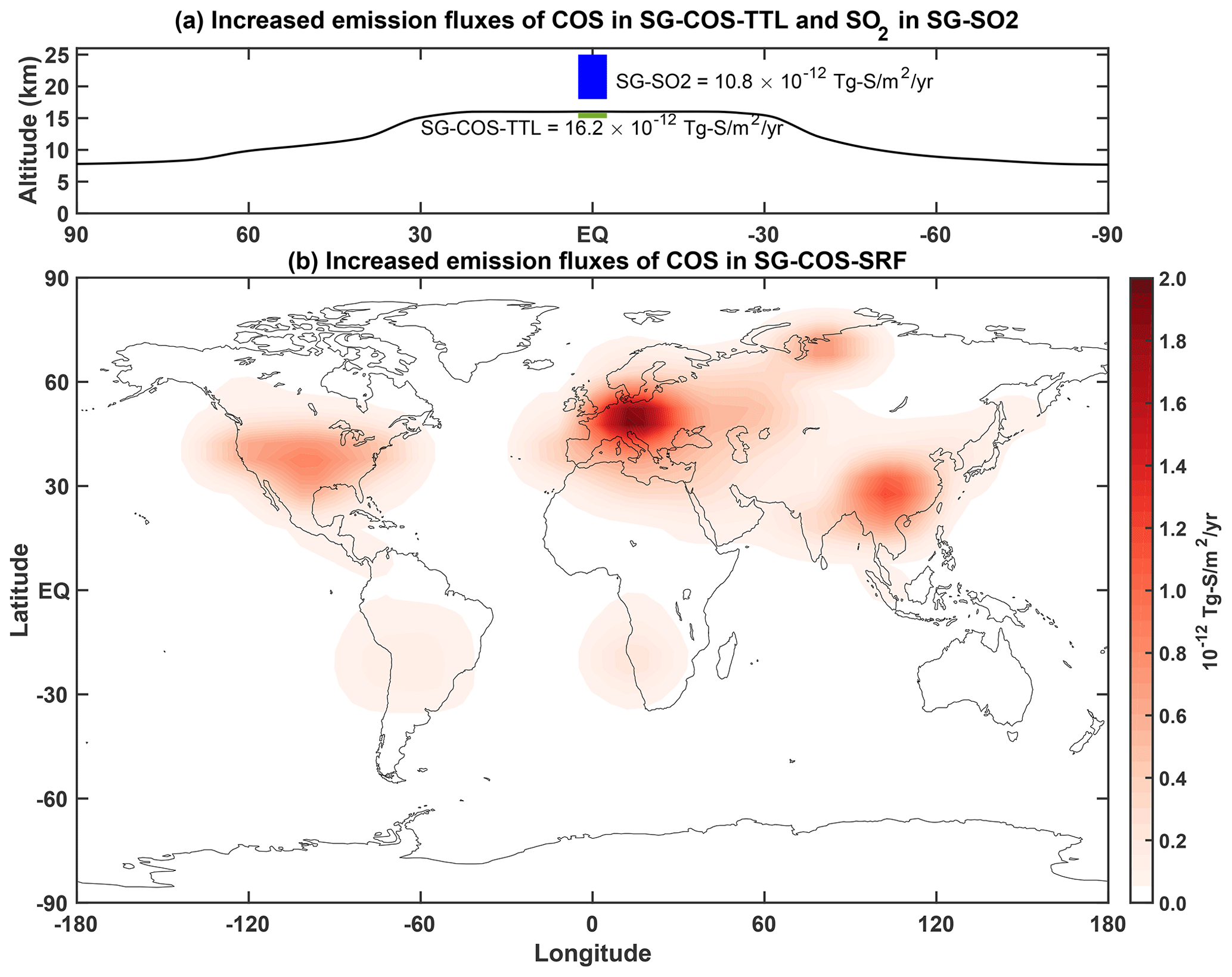
Figure 1 (a) Vertical and latitudinal distribution of COS emissions per year and unit of surface area (10⁻¹² $\mathrm{Tg}-\mathrm{S}{\mathrm{m}}^{-\mathrm{2}}{\mathrm{yr}}^{-\mathrm{1}}$) in the SG-COS-TTL experiment (green box) and SO₂ emission fluxes in the same unit in SG-SO2 (blue box). The quantities are distributed in a single vertical level for SG-COS-TTL and in 12 vertical levels for SG-SO2. (b) Geographical distribution of COS emission fluxes per year and unit of surface area (10⁻¹² $\mathrm{Tg}-\mathrm{S}{\mathrm{m}}^{-\mathrm{2}}{\mathrm{yr}}^{-\mathrm{1}}$) in the SG-COS-SRF experiment. The annual upward flux is averaged over the period 2046–2055.

For the geoengineering experiments, ULAQ-CCM is driven by time-dependent sea surface temperatures (SSTs) from the Community Climate System Model–Community Atmosphere Model version 4 (CCSM-CAM4; Neale et al., 2013), an atmosphere–ocean coupled model that ran similar geoengineering experiments to those in SG-SO2 (as described by Tilmes et al., 2015). This allows for the inclusion of the cooling produced by geoengineering on the surface for the assessment of the dynamical and chemical effect as simulated by ULAQ-CCM. To include the important radiative effects produced by other atmospheric components (mainly geoengineering-driven changes in greenhouse gas concentrations and in ice clouds; Visioni et al., 2017, 2018a), the radiative module of ULAQ-CCM calculates, at each time step, the surface temperature perturbation produced by the radiative flux changes induced by these components and includes them in the CCSM-CAM4 SSTs. This approach has been further explained and validated by Visioni et al. (2018a). While the prescribed SST set-up has been shown to correctly capture the dynamical changes produced by SRM (Visioni et al., 2017), it clearly does not capture the potential feedbacks that may be relevant for surface climate, such as those produced by the different latitudinal distribution of the aerosol optical depth that we will show later on. These differences may also, in turn, feed back onto changes in COS lifetime through precipitation changes (Whelan et al., 2016), which we cannot consider here. We will therefore limit ourselves to analysing the changes in atmospheric composition and dynamics and how those contribute to the overall radiative forcing from the aerosols. Future experiments with a more comprehensive Earth system model will be necessary to determine the full extent of the climatic response.

3 Results

3.1 Sulfate burden

COS is the most abundant sulfur-containing species in the atmosphere under quiescent conditions (i.e. not considering explosive volcanic eruptions). It is efficiently lost at the surface via dry deposition on soils and vegetation. Taking this sink into account, the net global lifetime (atmospheric chemistry plus surface deposition) is approximately 4 years, depending on the assumed magnitude of the soil and vegetation sink (Sandoval-Soto et al., 2005; Van Diest and Kesselmeier, 2008). In the troposphere, the COS chemical reactivity (mostly with the hydroxyl radical) is rather slow. COS is thus well mixed and is easily transported in the stratosphere through the tropical tropopause layer (TTL). In the mid-stratosphere, COS becomes efficiently photolysed by solar UV radiation, becoming an important source for stratospheric SO₂ and, finally, for sulfuric acid aerosols.

When increasing the surface emission fluxes in SG-COS-SRF, it takes ∼15 years before the concentration reaches a new equilibrium, from 0.5 to 35.5 ppbv (Fig. 2a), whereas, in SG-COS-TTL, the equilibrium value is 4.8 ppbv. In the same time span, the global AOD increases, reaching a value of 0.08 by 2035 in SG-COS-SRF and by 2030 in SG-COS-TTL, similar to the global value that is reached by the direct injection of SO₂ in the equatorial stratosphere in SG-SO2; in that case, however, the steady-state value is reached in only 1–2 years. In the GeoMIP G6sulfur experiment (Visioni et al., 2021b), the average global surface cooling reported by six Earth system models for a similar stratospheric OD (optical depth) was 0.46 K. At the end of 2055, the increased COS and SO₂ injections are stopped. Average tropospheric COS concentrations follow an exponential decay guided by the atmospheric lifetime (3.8 years due to chemistry but mainly due to soil deposition), reaching a value of 1.3 ppbv after 20 years in SG-COS-SRF (during 2075), whereas a similar value only takes 10 years to be reached in SG-COS-TTL. This means an increase of 0.8 ppbv, with respect to background condition, that would produce a direct radiative forcing (RF) that is negligible compared to other well-mixed greenhouse gases. The exponential decay of the stratospheric AOD in both SG-COS experiments is regulated by the stratospheric lifetime of COS (Fig. 2b), which is ∼10 years, and it is mainly due to the reaction with OH and photolysis, from which stratospheric SO₂ and finally sulfuric acid aerosols are formed. This is also combined with the depletion of the source of COS from the troposphere (Fig. 2a). Therefore, the e-folding time for stratospheric AOD is longer with respect to the one resulting from SG-SO2 (Fig. 2c). In 2075, the global stratospheric AOD reaches a value of 0.01 in the SG-COS experiments with respect to 0.003 in the background case.

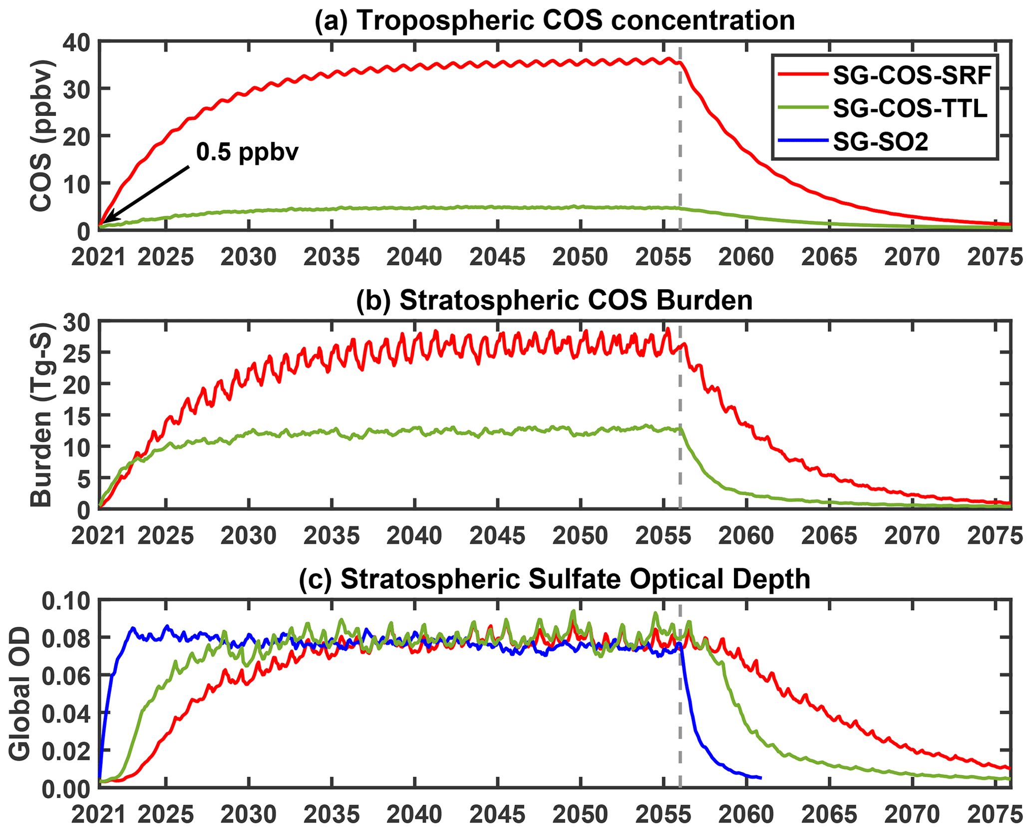
Figure 2 (a) Monthly values of globally averaged tropospheric COS volume mixing ratio (ppbv) in both SG-COS experiments. The background value of 0.5 ppbv at the beginning of the simulation is highlighted. (b) Monthly values of global stratospheric COS burden (in Tg-S) in both SG-COS experiments. (c) Globally averaged stratospheric sulfate optical depth monthly values in SG-COS-SRF (red), SG-COS-TTL (green), and SG-SO2 (blue). The grey line in all panels indicates the time when emissions of COS and SO₂ are stopped, which is at the end of 2055.

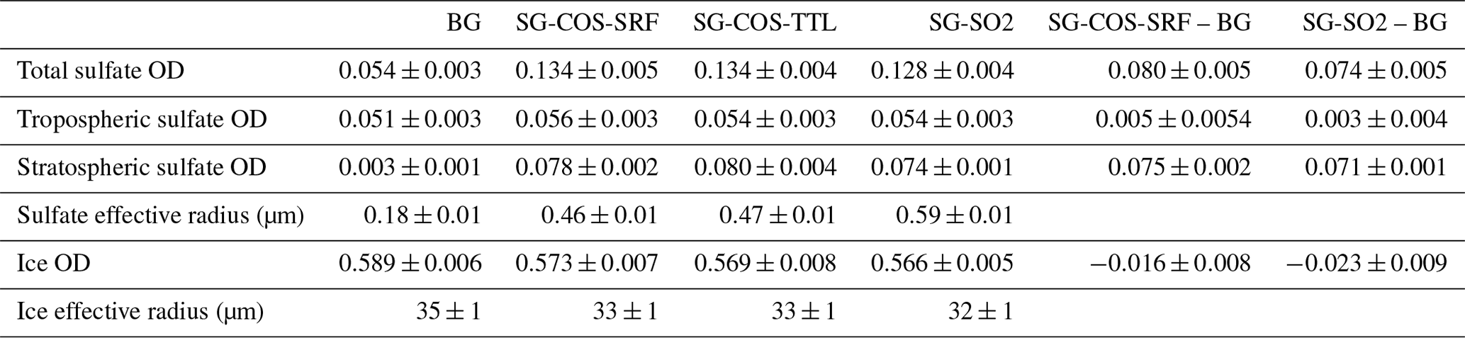
Table 1 Summary of the calculated sulfate aerosol and cirrus ice globally and annually averaged quantities relevant for RF calculations (i.e. optical depth at λ=0.55 µm and effective radius). The last two columns show the calculated SG changes with respect to the BG case (years 2046–2055).

3.2 Sulfate aerosol properties

In both COS experiments, COS emissions are adjusted so as to have the same global AOD ≈ 0.08 (see Table 1). This is done in order to more easily compare the latitudinal distribution of the aerosols and to better quantify the differences in the radiative forcing from both direct and indirect (ozone, methane, and water vapour) changes in atmospheric composition.

There is a large difference in the latitudinal distribution of stratospheric sulfate optical depth, as shown in Fig. 3a. Both SG-COS experiments produce an AOD that is more uniformly distributed over all latitudes with respect to the SG-SO2 case, where the increase in optical depth is most prominent in the tropics; this is due to the efficient tropospheric mixing of COS before it reaches the stratosphere even when, as in SG-COS-TTL, the injection happens close to the tropopause.

The differences in the latitudinal distribution of AOD are also observable in the differences in the particle sizes and in the surface area density (SAD). Figure 3b shows that the stratospheric effective radius is smaller in the SG-COS experiments and uniform for all latitudes, with a global value of 0.46 µm. In SG-SO2, the effective radius is higher in the tropics (0.59 µm). AOD is also larger in the tropics in that case, due to a larger concentration of particles there, even if larger particles are less effective at scattering incoming solar radiation (English et al., 2012).

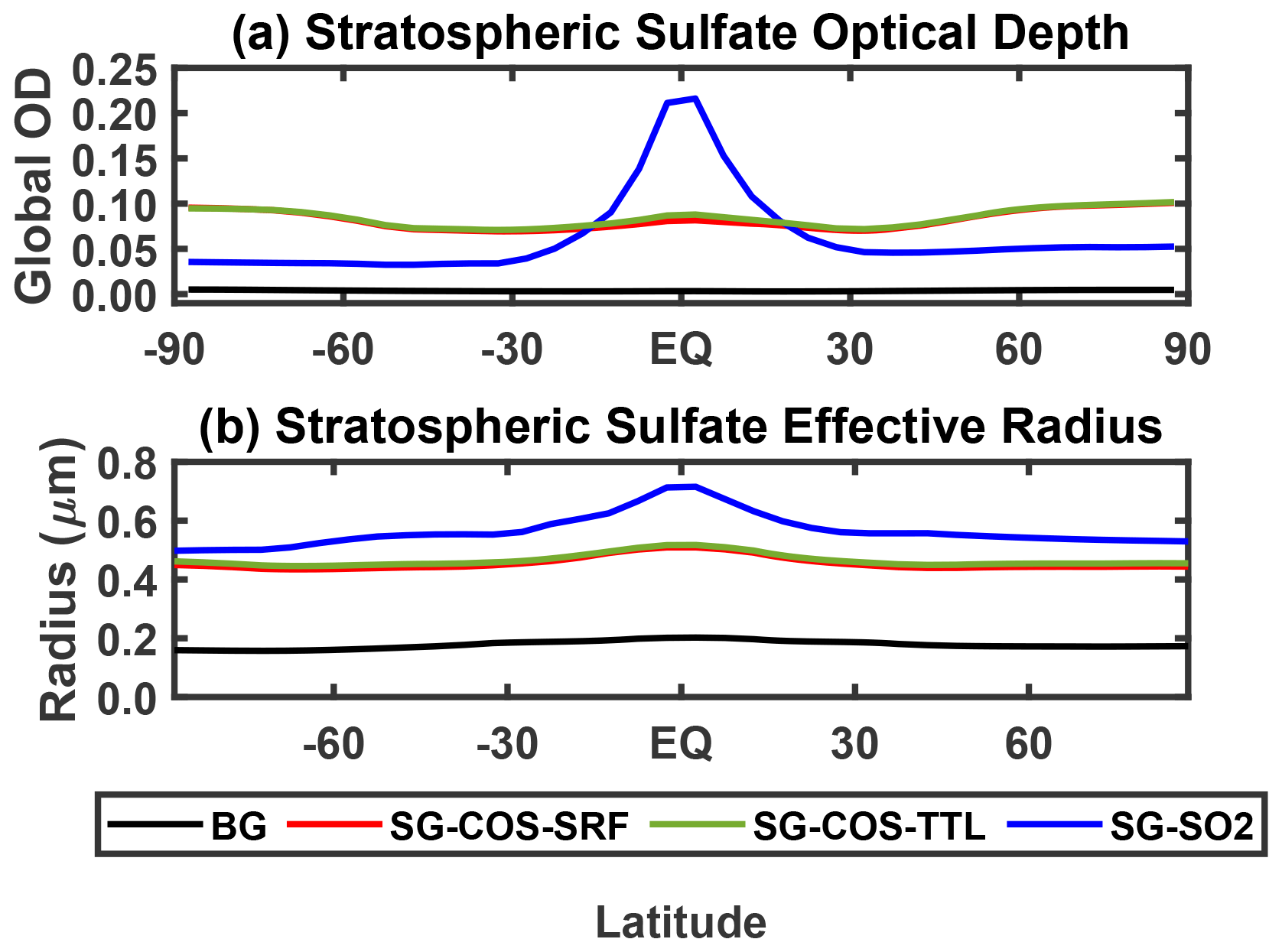
Figure 3 (a) Latitudinal distribution of zonal mean values of the stratospheric sulfate optical depth for the BG (black), SG-COS-SRF (red), SG-COS-TTL (green), and SG-SO2 (blue) cases. (b) Stratospheric effective radius (in µm, from the tropopause to 6 hPa). All quantities are annually averaged over the years 2046–2055.

Figure 4 shows a comparison of the effective radius (Fig. 4a) and SAD (Fig. 4b) between the BG, SG-COS-SRF, SG-COS-TTL, and SG-SO2 cases, separating the tropics, mid-latitudes, and polar regions. As SO₂ is injected at the Equator, all oxidation and nucleation happens in the tropics in SG-SO2. This is reflected in the vertical distribution, which has a maximum in the lowermost stratosphere. On the other hand, in SG-COS, the effective radius increase is reached at higher altitudes, between 18–30 km, which is consistent with COS reaching higher altitudes through deep tropical convection before it is photochemically destroyed (Barkley et al., 2008). The same explanation is valid for the tropical SAD in Fig. 4b.

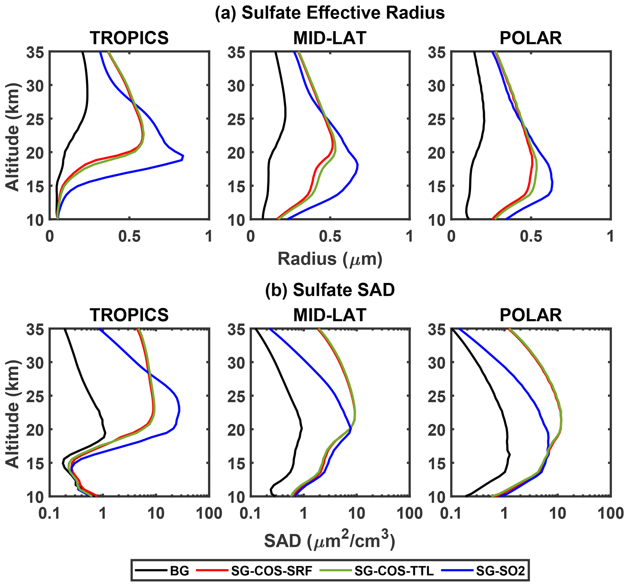
Figure 4 Vertical profiles of sulfate effective radius (in µm; a) and surface area density (in µm² cm⁻³; b) at different latitudinal bands (20^∘ N–20^∘ S for the tropics, 30–50^∘ at both N and S for the mid-latitudes, and 60–90^∘ at both N and S for the polar plots). All quantities are annually averaged over the years 2046–2055.

As the size of the particles is determined by nucleation in the tropical region, where SO₂ oxidation occurs, the mid-latitude and polar behaviour of the aerosols depends on the poleward transport by the Brewer–Dobson circulation (BDC).

In SG-SO2, aerosols grow rapidly in the tropical region due to the high concentration of SO₂, and their larger size affects sedimentation rates, thus decreasing their lifetime. Consequently, the number of aerosols transported to higher latitudes is lower; in SG-COS, smaller particles with a higher lifetime are either easily transported towards the poles or directly formed there. Smaller particles at a higher concentration and larger particles at a lower concentration may then result in a SAD, which looks similar at mid-latitudes and polar region but for different reasons.

The vertical distribution of particles and their optical properties are shown in Fig. 5 (see Fig. S2 in the Supplement for COS, SO₂, and SO₄ concentration changes; only values for one of the SG-COS experiments is shown here, as they are indistinguishable). The vertical distribution of the SAD is fundamental for understanding the role of the heterogeneous reaction and their effect on stratospheric ozone. The baseline cases in Fig. 5a and b are a reference for understanding their changes in the SG-COS experiments (Fig. 5c and d). The particles transported via the BDC to the poles are large enough to efficiently scatter the solar radiation so that the SAD and extinction changes show a similar behaviour, with a global increase of stratospheric values with maxima at higher latitudes between 15–25 km.

Figure 5 Zonal mean values of sulfate extinction (in 10⁻⁴ km⁻¹) and SAD (in µm² cm⁻³) in BG (panels a and b, respectively) and their change in the case of the SG-COS-SRF experiment (panels c and d). Panels (e) and (f) show extinction and SAD changes between SG-COS-SRF and SG-SO2. All quantities are annually averaged over the years 2046–2055.

Figure 5c and d show the extinction and SAD changes between the SG-COS and BG, same for Fig. 5e and f but between SG-COS the SG-SO2 to underline that, in SG-SO2, the extinction of the radiation is confined in the tropical stratosphere between 15–25 km, meaning that there is a negative change in SG-COS. As discussed before, the formation of larger particles in SG-SO2 in the tropical region reduces the amount of aerosol transported to the poles compared to the SG-COS cases, where a larger number of smaller particles produce a positive change in SAD and, consequently, in extinction.

3.3 Deposition

The enhancement of the stratospheric sulfate burden would produce an increase in sulfur deposition, both in dry form, through acid gas deposition, and in wet form, through rain, fog, and aerosol particles.

Acid deposition may damage human health when high concentrations of particles with a diameter below certain thresholds (PM_2.5 and PM₁₀) are inhaled. The acidification of soils and water may damage plants, microorganisms, and aquatic animals, but the impact on the ecosystem depends on the rate at which acidifying compounds are deposited from the atmosphere, compared with the rate at which acid neutralizing capacity is generated within the ecosystem (Driscoll et al., 2001).

Here we analyse how the dry and wet deposition of sulfur species are distributed globally as a result of the two SG interventions. Tables 2 and 3 summarize the wet and dry deposition rates for the SG-COS, SG-SO2, and BG experiments, and they include the contribution of each species to the total deposition. In particular, in both SG-COS experiments, the increase in COS fluxes produces both an increase in sulfuric deposition, after its photolysis and oxidation to sulfuric acid, and in the dry deposition of COS itself, as it is removed to the ground through uptake by vegetation and soils (Kettle et al., 2002).

Table 2 Globally and annually averaged dry deposition rates of sulfur species ($\mathrm{Tg}-\mathrm{S}{\mathrm{yr}}^{-\mathrm{1}}$; years 2046–2055). Note: MSA is methanesulfonic acid.

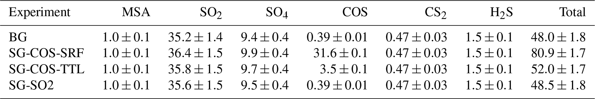
Table 3 Globally and annually averaged wet deposition rates of sulfur species ($\mathrm{Tg}-\mathrm{S}{\mathrm{yr}}^{-\mathrm{1}}$; years 2046–2055). The last column shows the net balance of total sulfur sources and sinks ($\mathrm{Tg}-\mathrm{S}{\mathrm{yr}}^{-\mathrm{1}}$).

The global distribution of COS deposition for the baseline case is shown in Fig. 6a, while the increase in deposition from the SG-COS-SRF experiment is shown in Fig. 6b. For the SG-COS-TTL case, the spatial distribution is identical to SG-COS-SRF, but its magnitude is 10 times lower than in SG-COS-SRF. COS uptake by plants is concentrated mainly in the tropical rainforests of South America, Africa, and southeast Asia and boreal coniferous forests across North America, northern Europe, and northern Asia. Uptake by soils occurs mainly in arid and semiarid regions, such as savanna regions in northern and southern Africa and in the southwestern regions of North America, in the pampas of Argentina, in Australia, and in the steppes of central Asia (Kettle et al., 2002). Dry deposition of COS does not contribute to acid deposition, and currently, there is no information available on how different soils or ecosystems would be affected by higher local COS concentrations; therefore, we assumed that their uptake efficiency does not change. The robustness of this assumption will need to be studied.

The global distribution of SO_x deposition is also shown in Fig. 6c and d, which show dry and wet deposition, respectively, for the background case. Dry deposition maxima are localized in urban areas close to the source where the emitted sulfur dioxide is immediately oxidized, while wet deposition distribution depends both on sulfate concentration and precipitation.

Figure 6e and f show the total SO_x deposition change in SG-COS-SRF with respect to the baseline case, both in absolute terms and as a percentage of the baseline case, and most of its increase is due to wet deposition (see Tables 2 and 3; see Tables S1–S4 for a breakdown of global sources and sinks of sulfur species). In both figures, the distribution of deposition is more uniform over the globe with respect to the tropical injection of SO₂, except for the polar regions, because of the reduced precipitation rates. Consequently, Fig. 6f shows a large increase in percent deposition in the polar region (17 % in the Arctic and 8 % in Antarctic; these values are reduced to 1.7 % and 0.8 % in SG-COS-TTL; see Fig. S4) because of very low values in the baseline case. On the other hand, the deposition change is close to zero in polluted regions.

Globally, the annual differences in deposition fluxes for all species, compared to the background case, amount to 8.3±0.2 $\mathrm{Tg}-\mathrm{S}{\mathrm{yr}}^{-\mathrm{1}}$ for SG-COS-SRF and 3.1±0.2 and 3.9±0.2 $\mathrm{Tg}-\mathrm{S}{\mathrm{yr}}^{-\mathrm{1}}$ for SG-SO2, which equates to an increase of 8.9 %±0.3 %, 3.3 %±0.3 %, and 4.2 %±0.3 %, respectively.

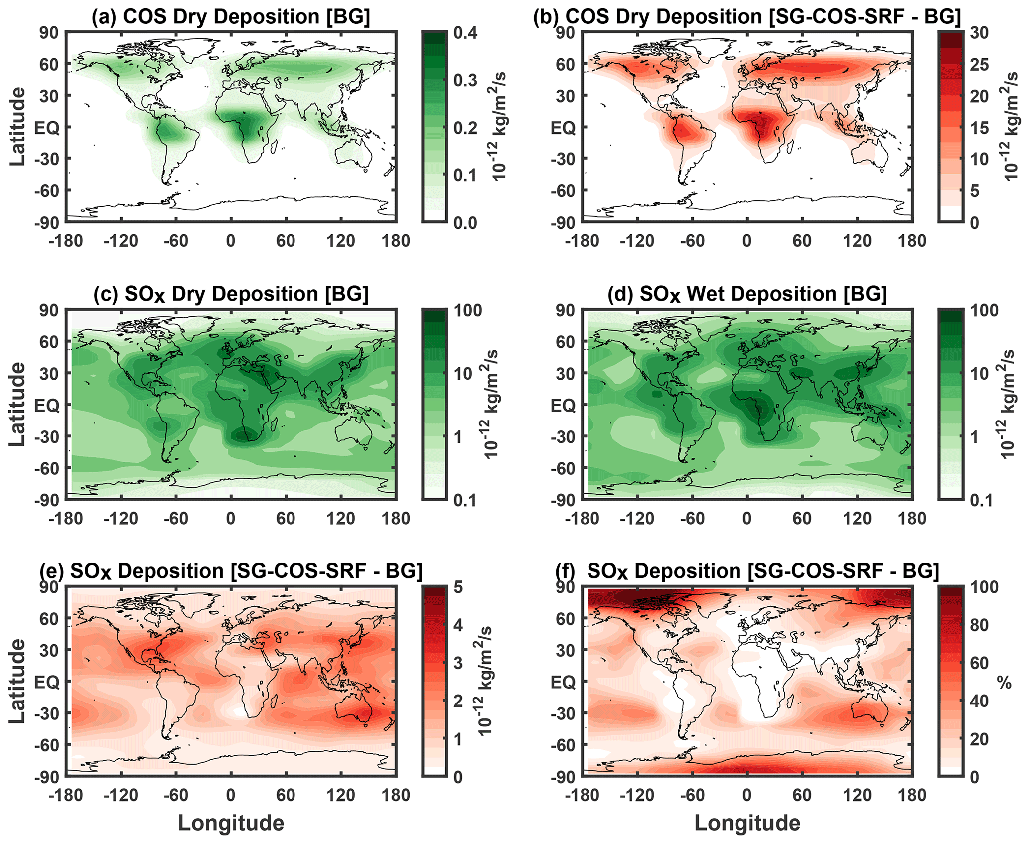
Figure 6 (a) Surface dry deposition fluxes (10⁻¹² $\mathrm{kg}{\mathrm{m}}^{-\mathrm{2}}{\mathrm{s}}^{-\mathrm{1}}$) of COS in the background case. (b) Change in COS dry deposition fluxes in SG-COS-SRF compared to panel (a). (c) SO_x dry deposition fluxes (10⁻¹² $\mathrm{kg}{\mathrm{m}}^{-\mathrm{2}}{\mathrm{s}}^{-\mathrm{1}}$) in the background case. (d) SO_x dry deposition fluxes (10⁻¹² $\mathrm{kg}{\mathrm{m}}^{-\mathrm{2}}{\mathrm{s}}^{-\mathrm{1}}$) in the background case. (e) Change in SO_x total deposition fluxes in SG-COS-SRF compared to the background. Panel (f) is the same as panel (e) but in percent of the background values.

4 Indirect effects

The simulated enhancement in the stratospheric aerosol layer would produce two main effects, namely an increased scattering of solar radiation that, in turn, would reduce surface temperatures, and the local absorption of more near-infrared solar and terrestrial radiation that would warm the stratospheric layer where the aerosols reside (as observed for volcanic eruptions; see Lacis et al., 1992; Labitzke and McCormick, 1992). Furthermore, the increase in the surface area density of the aerosols would affect the heterogeneous chemistry of ClO_x and NO_x, with implications for ozone concentration and UV radiation at the surface (Tilmes et al., 2009, 2018b, 2021).

For SO₂, it has been shown that the combination of surface cooling, perturbation of stratospheric temperatures, and changes in tropospheric ozone and in UV at the surface also affect methane lifetime (Visioni et al., 2017). In this section, we analyse the differences in these changes also for the SG-COS-SRF experiment.

Figure 7 shows the ozone changes in SG-COS-SRF and SG-SO2 with respect to the BG case. As expected from the similar value and distribution of the SAD, in SG-COS-TTL, the ozone changes are equivalent to SG-COS-SRF (and are therefore not shown). Figure 7a and b show the monthly total ozone column changes as a function of latitude. Close to the Equator, there is a small reduction in the overall column, mostly due to a reduction in tropospheric ozone, as visible in Fig. 7c and d, as a direct consequence of the surface cooling (Nowack et al., 2016). On the other hand, at higher latitudes, an overall increase in the total column is observable due to an increase in stratospheric ozone. This is particularly evident closer to the poles.

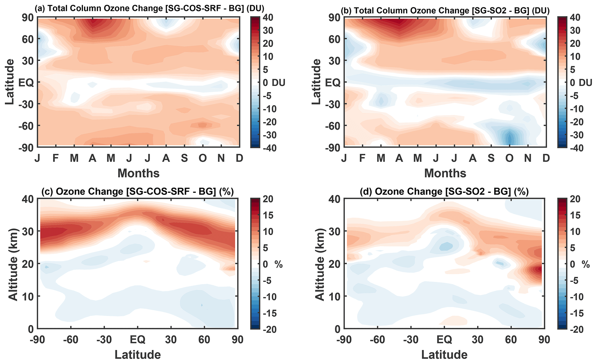
Figure 7 (a, b) Monthly mean zonal values of the SG ozone total column changes (DU) with respect to the BG case for SG-COS-SRF and SG-SO2, respectively. (c, d) Ozone mixing ratio percent changes with respect to the BG case. All quantities are annually averaged over the years 2046–2055.

During springtime months, there is some Antarctic ozone depletion, while in the Arctic a recovery of ozone is observable. In the Antarctic spring, the polar vortex is strengthened by the stratospheric heating in the tropics that affects the Equator-to-pole thermal wind balance (Visioni et al., 2020), resulting in greater confinement of cold air that, in turn, enhances the ozone depletion by the polar stratospheric clouds (PSCs). The tropical stratospheric heating is higher in SG-SO2 with respect to SG-COS, as the aerosols are less confined (Fig. S6). Consequently, the strengthening of polar vortex in SG-SO2 produces a higher ozone depletion. In the Arctic, on the other hand, PSC-related ozone loss is lower (Tilmes et al., 2018a), and the predominant effect is that from an acceleration of the BDC transporting ozone-rich air from lower latitudes.

Figure 7c and d show the annual mean of the ozone mixing ratio percentage change as a function of altitude and latitude. In both SG experiments, negative changes below the tropopause are governed by the decrease in solar radiation which comes into play in the photo-dissociation reaction of NO_x as an ozone precursor (${\mathrm{NO}}_{\mathrm{2}}+h\mathit{\nu }(\mathit{\lambda }<\mathrm{420}\mathrm{nm})\to \mathrm{NO}+\mathrm{O}{(}^{\mathrm{3}}\mathrm{P})$). Sunlight reduction also affects the O₃ photolysis, decreasing the ozone loss. Positive changes are due to the balance of the previous reactions and the increase in methane (see Table 4) as a source of ozone in its oxidation chain and mainly due to the decrease in the tropospheric water vapour in a clean air environment (low NO_x), such as the tropics (Nowack et al., 2016; Xia et al., 2017).

Table 4 Summary of calculated globally and annually averaged quantities of greenhouse gases directly and indirectly perturbed by SG and relevant for RF calculations (i.e. COS mean tropospheric mixing ratio, CH₄ atmospheric lifetime, H₂O mean stratospheric mixing ratio, and O₃ column). The last two columns show the calculated SG changes with respect to the BG case (years 2046–2055). Note: ppmv is parts per million by volume.

Above the tropopause, there is a negative ozone change in the lower stratosphere in all SG experiments, except for the Arctic region, where we observe a small increase in the Arctic lowermost stratosphere in all cases. The key drivers of the stratospheric ozone change are the increase in heterogeneous reactions as a result of the enhancement of stratospheric aerosols and the perturbation of the dynamics governing ozone transport.

Negative ozone changes correspond to the region where the SAD reaches its maximum values (Fig. 5d and f), i.e. between 10–20 km in the polar regions for SG-COS and mainly between 15–25 km at tropics for SG-SO2. The increase in the SAD enhances heterogeneous chemistry and results in denitrification via hydrolysis of dinitrogen pentoxide (${\mathrm{N}}_{\mathrm{2}}{\mathrm{O}}_{\mathrm{5}}+{\mathrm{H}}_{\mathrm{2}}\mathrm{O}\stackrel{\text{M}}{⟶}\mathrm{2}{\mathrm{HNO}}_{\mathrm{3}}$). The loss of NO_x decreases the rate of ozone depletion through its catalytic cycle. Whereas, in the mid-stratosphere, where the cycles of chlorine (ClO_x) and bromine (BrO_x) are dominant, there is an increase in ozone loss since there is a reduction in NO_x that normally bounds chlorine (ClONO₂), thus allowing more ClO-driven ozone destruction (Tilmes et al., 2018b; Grant et al., 1992).

At low latitudes, stratospheric ozone concentration is also driven by changes in tropical upwelling (Visioni et al., 2021a). The reduction in the tropical upwelling of ozone-poor air coming from the lowermost stratosphere leads to higher ozone concentration at altitudes of about 20–22 km (Tilmes et al., 2018b).

Figure S7e shows the change in tropical upwelling in relation to changes in the residual vertical velocity (w^*) with respect to the baseline case. Negative w^* anomalies in SG-COS mean weaker tropical upwelling as a consequence of tropospheric cooling. In SG-SO2, the highest concentration of absorbing aerosols leads to positive w^* above 20 km due to the local warming, but this does not affect the transport of ozone-poor air from the lower layers.

Above the discussed altitudes, there is a net ozone production in all SG experiments, with a higher increase in the ozone mixing ratio in the SG-COS experiment with respect to SG-SO2, especially in the extra-tropical region. Ozone depletion at these altitudes is mainly controlled by the catalytic cycle of NO_x that is inhibited by the denitrification process due to heterogeneous reactions on aerosols.

Globally, the annually averaged ozone column increases by ∼5 and 1.5 DU for SG-COS and SG-SO2, respectively (Table 4). Increasing stratospheric ozone affects ultraviolet B (UVB) at the surface because it is absorbed by ozone during its photodissociation, while aerosol could affect ultraviolet A (UVA) radiation by scattering processes. The projected changes are shown in Fig. 8 for both UVA and UVB for each season and for the annual mean. We estimated these changes using the tropospheric ultraviolet and visible (TUV) radiation model (from https://www2.acom.ucar.edu/modeling/tropospheric-ultraviolet-and-visible-tuv-radiation-model, last access: 29 April 2022), using as input our model latitudinal and monthly values for the period of 2046–2055, for aerosol optical depth, total ozone column, climatological cloud cover, and surface albedo.

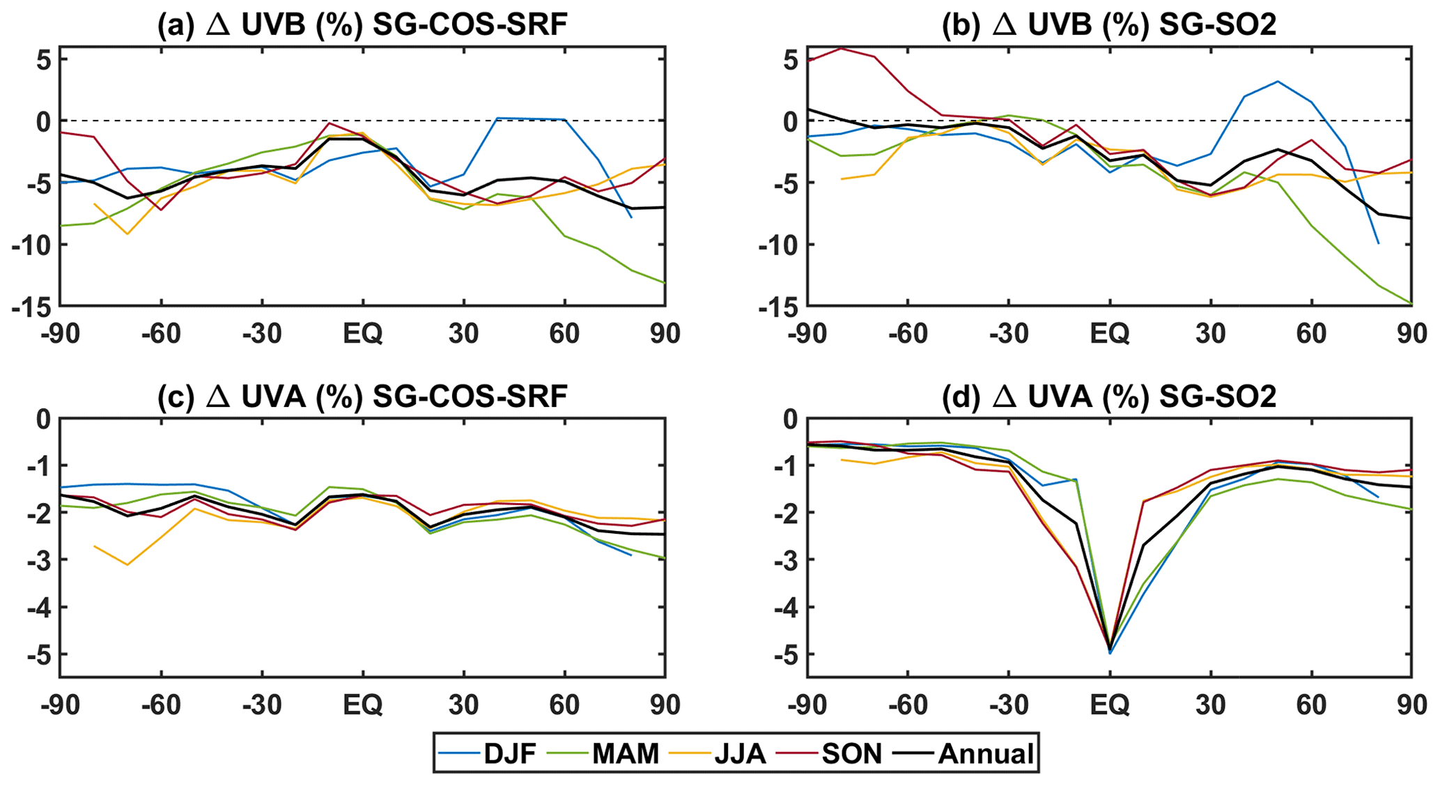
Figure 8 Zonal UVB and UVA surface changes per each season in percentage with respect to BG case in SG-COS-SRF (a and b, respectively) and SG-SO2 (c, d). All quantities are averaged over the years 2046–2055.

In all SG experiments, the negative changes of UVB radiation at the surface, except in the Antarctic region, are related to changes in stratospheric ozone and the interannual variations that are larger at the poles, due to the seasonal variability, as discussed before. In the Antarctic spring (September–November; SON) the ozone depletion is enhanced in SG-SO2, while in SG-COS-SRF it is limited to the month of October, with differences compared to BG of less than −5 DU. Therefore, the UVB change compared to BG for SON over Antarctica remains negative in SG-COS-SRF, with a value of −2.7 % versus a +5.8 % increase in the SG-SO2 experiment. In DJF (December–February), on the other hand, a small increase in UVB is observable at mid- to high latitudes in the Northern Hemisphere. This is connected to an observable decrease in stratospheric ozone in the same locations, possibly due to a reduced advection of air from the tropics. UVA decreases everywhere in all SG experiments. In particular, the correlation between UVA change and particles scattering is evident if we compare this latitudinal distribution with the stratospheric AOD of Fig. 3a. The globally averaged UVB and UVA changes at surface are summarized in Table 5.

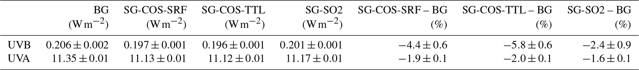
Table 5 Summary of calculated globally and annually averaged quantities of UVB and UVA at surface. The last two columns show the calculated SG percentage changes with respect to the BG case (years 2046–2055).

Methane is an indirect source of tropospheric ozone (West and Fiore, 2005), and it is also a greenhouse gas. Knowing its variation is fundamental for understanding the final contribution to the radiative forcing that one would wish to achieve with this geoengineering method. From Table 4, we find a global increase in methane lifetime of ∼13 % in SG-COS and 12.2 % in SG-SO2, which we can identify in the increase in methane itself. The reason for the increase in methane is to be found in the behaviour of the hydroxyl radical (OH), as the main sink of methane is the oxidation reaction with OH; a decrease in OH means an increase in the methane lifetime. As discussed by Visioni et al. (2017), mechanisms that cause an increase in OH are as follows: (a) surface cooling lessens the amount of tropospheric water vapour and inhibits the temperature-dependent reaction of NO+O₃; (b) a decrease in tropospheric UV, due to enhancement of ozone and scattering radiation, reduces O(¹D) that takes part of the reaction $\mathrm{O}{(}^{\mathrm{1}}\mathrm{D})+{\mathrm{H}}_{\mathrm{2}}\mathrm{O}\to \mathrm{2}\mathrm{OH}$; (c) an increase in SAD enhances the heterogeneous chemistry, reducing the amount of NO_x (NO+HO₂, NO+RO₂); (d) a increase in the tropical lower stratosphere temperature (TTL) that regulates the stratosphere–troposphere exchange, which can be positive or negative, depending on the net result of the superimposed species (CH₄, NO_y, O₃, and SO₄) in the extratropical upper troposphere–lower stratosphere (UTLS).

The warming of the TTL is shown in Fig. S7d. In SG-SO2, larger particles confined in the tropical region produce a greater warming of the TTL with respect to smaller ones distributed all over the globe in SG-COS. The role of the dimensions and distributions of aerosols in stratospheric warming is confirmed by the heating rates, as shown in Fig. S6.

5 Radiative forcing

The ULAQ-CCM radiative transfer module calculates online the radiative forcing due to aerosols, greenhouse gases (GHGs), and low and high clouds. The effects of single components have been estimated offline for both shortwaves (SWs) and longwaves (LWs) with the same radiative transfer core, for sulfate aerosols, clouds, COS, CH₄, stratospheric H₂O, and stratospheric and tropospheric O₃ in order to properly separate the contributions.

Tables S8–S10 in the Supplement summarize the individual contributions of GHGs changes for SG-COS-SRF, SG-COS-TTL, and SG-SO2, respectively. Similar increases in methane in all SG experiments produce the same positive LW RF; the TTL warming (which results in an increase in stratospheric water vapour), results in a small but positive contribution from H₂O in SG-SO2. Contributions from both stratospheric and tropospheric O₃ changes have also been estimated but are negligible.

In both SG-COS experiments, obviously, the increase in COS concentration, which is a GHG, must be taken into account. We estimated its contribution to the radiative forcing based on the definition of global warming potential (GWP) on a mass/mass basis, as in Brühl et al. (2012), for a time horizons of 30 years (2021–2050). GWP can be approximated, as follows, by the expression of Roehl et al. (1995), assuming that the perturbation of the radiation balance of the Earth by greenhouse gases COS and CO₂ decays exponentially after a pulse emission for a time horizon ΔT.

$$\begin{array}{}\text{(1)}& {\text{GWP}}_{\mathrm{\Delta }t}\simeq {\displaystyle \frac{{\text{RF}}_{\text{COS}}}{{\text{RF}}_{{\mathrm{CO}}_{\mathrm{2}}}}}\times {\displaystyle \frac{{\mathit{\tau }}_{\text{COS}}}{{\mathit{\tau }}_{{\mathrm{CO}}_{\mathrm{2}}}}}\times {\displaystyle \frac{\mathrm{1}-e^{\frac{-\mathrm{\Delta }t}{{\mathit{\tau }}_{\text{COS}}}}}{\mathrm{1}-e^{\frac{-\mathrm{\Delta }t}{{\mathit{\tau }}_{{\mathrm{CO}}_{\mathrm{2}}}}}}}.\end{array}$$

We assumed an overall lifetime of τ_COS=3.8 and ${\mathit{\tau }}_{{\mathrm{CO}}_{\mathrm{2}}}=\mathrm{75}$ years, and the radiative forcing of 1 kg of COS relative to 1 kg of CO₂ added to the present atmosphere (${\text{RF}}_{\text{COS}}/{\text{RF}}_{{\mathrm{CO}}_{\mathrm{2}}}$) is 724 (Brühl and Crutzen, 1988). This results in a GWP of 111. For our time period, the mass of COS and CO₂ added to the atmosphere (Δm) is 1.97×10¹² kg of COS (for SG-COS-SRF), 0.35×10¹² kg of COS (for SG-COS-TTL), and 1.23×10¹⁵ kg of CO₂. Therefore, the COS radiative forcing can be calculated as follows:

$$\begin{array}{}\text{(2)}& {\text{RF}}_{\text{COS}}={\text{GWP}}_{\mathrm{\Delta }t}\times {\text{RF}}_{{\mathrm{CO}}_{\mathrm{2}}}\times {\displaystyle \frac{\mathrm{\Delta }{m}_{\text{COS}}}{\mathrm{\Delta }{m}_{{\mathrm{CO}}_{\mathrm{2}}}}},\end{array}$$

where ${\text{RF}}_{{\mathrm{CO}}_{\mathrm{2}}}$ in RCP6.0 is estimated to be 0.83 W m⁻², considering an increase of 68.5 ppm from a baseline of 409.2 ppm. Overall, this results in a radiative forcing from the COS increase of 0.17 W m⁻² in SG-COS-SRF and of 0.03 W m⁻² in SG-COS-TTL.

The main contributions of sulfate aerosols and clouds are summarized in Tables S5–S7 in the Supplement for SG-COS-SRF, SG-COS-TTL, and SG-SO2, respectively. The contribution of sulfate aerosols is the sum of the cooling effects given by the efficient scattering of solar radiation by particles of radius of around 0.5 µm and the absorption of LW by larger ones. Globally, the estimated values are similar for the clear-sky SW and LW forcing from the sulfate aerosols. In terms of the latitudinal distribution, however, SG-SO2 presents a peak in the tropics, whereas the forcing from SG-COS is much more latitudinally even.

The reduction in optical depth from cirrus clouds (see Table 1) produced by the aerosols (Kuebbeler et al., 2012; Visioni et al., 2018a) results in a net negative radiative forcing. This is given by the balance between the positive RF in the shortwaves (SWs), due to the reduction of reflected solar radiation, and the negative RF in the longwaves (LWs), due to the decrease in the trapped planetary radiation, which reduces the contribution to the greenhouse effect. In the SG-COS cases, at the Equator, the positive RF, from the cirrus ice thinning, locally balances the direct forcing from the aerosol (Figs. 9 and S8 in the Supplement).

Table 6 summarizes the total contribution of sulfate aerosols and greenhouse gases under all-sky conditions.

Table 6 Globally and annually averaged total RF of sulfate aerosols and greenhouse gases for the SG experiments with respect to BG (shortwave, longwave, and net; W m⁻²; years 2046–2055).

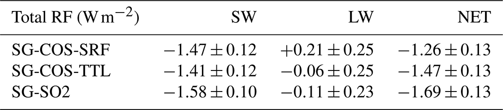
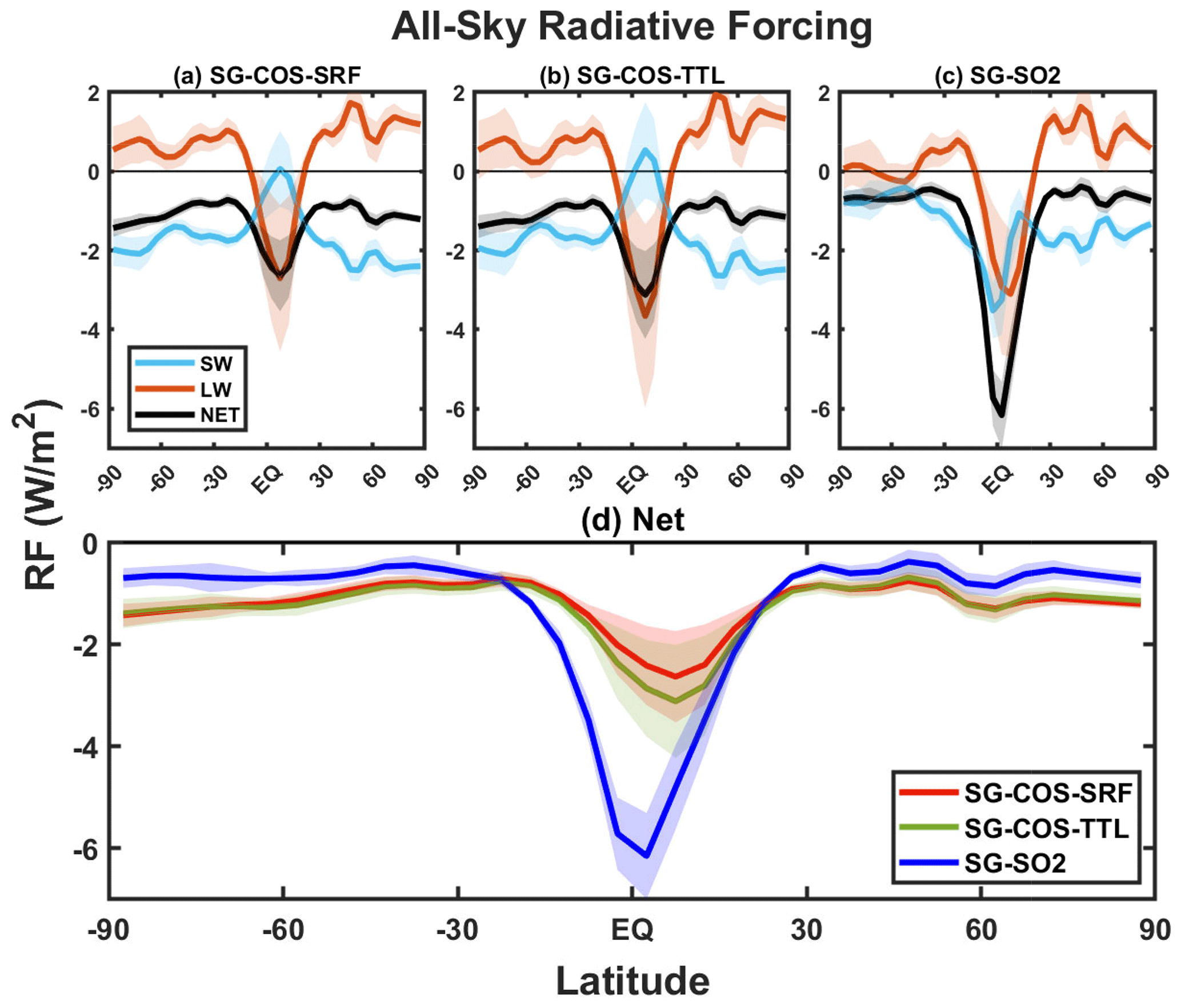
Figure 9 (a–c) Mean zonal shortwave (cyan), longwave (orange), and net (black) all-sky radiative forcing (in W m⁻²) in SG-COS-SRF, SG-COS-TTL, and SG-SO2, respectively. (d) Comparison of the net radiative forcings from SG-COS-SRF (red), SG-COS-TTL (green), and SG-SO2 (blue). All quantities are annually averaged over the years 2046–2055. Shadings in all panels represent 1 standard deviation in the interannual variability.

6 Technical feasibility of SG through COS emissions

We briefly discuss here the technical feasibility of the approach described in this paper, as it is mainly related to the increase in surface COS emissions (for SO₂ injections; see, for instance, Smith and Wagner, 2018; Smith et al., 2020).

Patent number 3 409 399 (1968) has developed a method for the high yield synthesis of COS (93.2 %–96.6 %) as follows:

$${\mathrm{CO}}_{\mathrm{2}}+{\mathrm{CS}}_{\mathrm{2}}\stackrel{\mathrm{100}-\mathrm{600}{}^{\circ }\mathrm{C}}{⟶}\mathrm{2}\mathrm{COS}.$$

CO₂ is abundant, even in concentrated (90 %+) streams, from various natural and industrial sources, particularly with cooperation from states or industries. For example, capturing flue gas from coal-fired power plants is an established technology and may yield over 90 % CO₂ (Wang et al., 2013). CS₂ is produced via numerous means, perhaps the easiest being from coke (carbon) and molten sulfur, as follows:

$$\mathrm{C}+\mathrm{2}\mathrm{S}\stackrel{\text{high temperature}}{⟶}{\mathrm{CS}}_{\mathrm{2}}.$$

Approximately 1×10⁶ t of CS₂ is produced per year (Madon and Strickland-Constable, 1958), with China consuming approximately half of the global production of CS₂ for rayon manufacture. CS₂ is highly unstable and is flammable in air. It is also toxic at low concentrations (10 ppm).

Given the reactions above, about 0.5 Tg of S will produce 0.94 Tg of COS. This amounts to 0.16 Tg of C (coke) and 0.55 Tg of molten sulfur. In the last decade, approximately 70 Tg of sulfur were produced worldwide, so this would constitute an increase in S production of 0.8 %. The price varied between USD 50 and USD 200 per tonne, leading to an annual cost of approximately USD 25 million–USD 100 million. The worldwide production of coke was around 640 Tg, so this increase in production is negligible. The price of coke varies between USD 50 and USD 100 per tonne, leading to an annual cost of approximately USD 8 million–USD 16 million. To this we would have to add the cost of CO₂, in addition to the production and energy costs. Considering an estimate of USD 400 million per year for each Tg of S between CO₂ and production and energy cost, and assuming an effort shared between 1000 locations, this would add up to USD 400 000 per location per year per each Tg of S. The overall cost is roughly of the same order of magnitude as that in Smith and Wagner (2018), for a stratospheric aerosol deployment at ∼20 km of injection (so different from the injection set-up in our study for SG-SO2), but without the need to develop a new aircraft-based delivery system. For the SG-COS-TTL case, the overall cost would be a combination of the production costs of COS, as described above (but almost 10 times less per year to obtain the same AOD as SG-COS-SRF), and those of a deployment in the upper troposphere, which may result in being less expensive than a deployment in the lower stratosphere, as needed for SO₂.

7 Conclusions

We have presented here the results of a modelling experiment with the aim of producing an optically thick cloud of sulfate aerosols in the stratosphere without the injection of sulfate precursors directly into the stratosphere but rather by using increased surface or upper tropospheric emissions of carbonyl sulfide (COS). The low reactivity of COS in the troposphere, where it is not reactive and where it is predominantly absorbed by some soils and by plants, allows for a large portion of its emissions to reach the stratosphere, where it is turned into sulfate aerosols by photo-dissociation and oxidation.

We compare the results obtained in the following injection scenarios: (i) 40 $\mathrm{Tg}-\mathrm{S}{\mathrm{yr}}^{-\mathrm{1}}$ of COS injected from the surface (roughly 400 times more than the background emissions), (ii) 6 $\mathrm{Tg}-\mathrm{S}{\mathrm{yr}}^{-\mathrm{1}}$ of COS injected in the equatorial upper troposphere (15 km), and (iii) 4 $\mathrm{Tg}-\mathrm{S}{\mathrm{yr}}^{-\mathrm{1}}$ of SO₂ injected in the equatorial stratosphere, as prescribed in previous experiments (Kravitz et al., 2011; Visioni et al., 2017). All experiments result in a similar global optical depth from the produced stratospheric aerosols (∼0.08) but with different latitudinal distributions. For SO₂, as previously observed in various modelling experiments, equatorial injections result in an increased concentration of aerosols in the tropical stratosphere that tends to overcool the tropics and undercool the high latitudes (Kravitz et al., 2018; Jiang et al., 2019), while also reducing the efficacy of the backscattering from the aerosols due to the increased size of the particles (Visioni et al., 2018b). On the other hand, with COS emissions, independently from the injection height, the uniform mixing of the gas allows for a more uniform distribution of the produced aerosols in the stratosphere, resulting in increased optical depth also at very high latitudes.

The differences in the distribution and size of the particles result in different changes to the composition of the atmosphere. Smaller particles absorb and heat the stratosphere less, thus resulting in fewer dynamical changes. From a chemical perspective, stratospheric ozone would be impacted differently from the two geoengineering schemes. For SO₂ injections, previous studies have shown that the overall effect is the result of a combination of various dynamical and chemical factors that behave differently, depending on the latitude and altitude of the aerosols. At low latitudes, the increase in lower stratospheric water vapour produced by the warming of the tropopause layer enhances the halogen-driven destruction of ozone in the lower stratosphere (Tilmes et al., 2018b) due to NO_x depletion. This effect is balanced by reduced ozone destruction in the middle stratosphere due to the slowing down of the NO_x cycle produced by enhanced heterogeneous chemistry (Pitari et al., 2014; Richter et al., 2017; Franke et al., 2021).

Overall, in the case of COS emissions, the further increase in surface area density produced by smaller particles increases the inhibition of the ozone cycles in the middle stratosphere, resulting in a net increase in stratospheric ozone and, thus, in a larger decrease in UV radiation at the surface. Similarly, the larger sulfate burden at high latitudes produces further ozone recovery and thus also less UV radiation at the poles for the COS case.

Our results point to the feasibility of increased emissions of COS as a possible substitute to stratospheric SO₂ (or other sulfate precursors) injections to produce stratospheric sulfate aerosols. Surface emissions would sidestep the problem of deploying methods not already available to bring the sulfate at those altitudes, including the development of novel aircraft (Bingaman et al., 2020). Since COS is already a byproduct of human activities, it might be possible to devise methods of mass production of the required quantities that may be cheaper than the known proposed methods (Smith et al., 2020). However, this strategy necessitates a larger amount of emissions to achieve the same global stratospheric AOD, resulting in larger amounts of deposition. Furthermore, while the toxic levels of COS concentrations are orders of magnitude larger than the one achieved in our simulation (Kilburn and Warshaw, 1995; Bartholomaeus and Haritos, 2006), the effects of prolonged exposure to lower concentrations would have to be assessed; the effect of increased COS concentrations on ecosystems would also require careful investigation. Estimations of the tropospheric radiative effect would also need to be refined to make sure that it is not larger than previously estimated, thus reducing the efficacy of the aerosol-induced cooling. We have shown that tropospheric injections of lower quantities of COS would produce the same optical depth and indirect effects while resulting in an increase in tropospheric COS concentrations 10 times lower than those with surface emissions. This would, however, still require the deployment of an aircraft fleet as in SO₂ emissions, but the technical challenges of reaching 15 km might be less than those faced when reaching 20 km Smith et al. (2020).

Overall, there may be other weak points in the geoengineering strategies using COS emissions compared to SO₂ that need to be addressed. They would be less easily scalable, and both the deployment and phaseout, as we have shown, would require a longer time frame compared to the almost instantaneous effect produced by SO₂ injections. Considering the dangers to ecosystems presented by a too fast deployment or termination of sulfate geoengineering (Trisos et al., 2018), this might not actually be a large drawback, but it does remove the possibility of rapidly regulating the necessary amount of stratospheric sulfate in case of changes in strategy or external conditions (such as a Pinatubo-like volcanic eruption; Laakso et al., 2016). The comparison between our two COS experiments suggests that the mixing happening in the troposphere would not allow any control in the latitudinal or seasonal distribution of the resulting aerosols, as proposed elsewhere for SO₂ injections (MacMartin et al., 2017; Dai et al., 2018; Visioni et al., 2019); however, future investigations may expand on this work by exploring whether a different combination of injection altitudes and locations may offer at least some control over the aerosol cloud.

Clearly, this study is intended to be just a pilot study of this method, and further simulations with other climate models, possibly with a coupled ocean and interactive land model to determine the full surface response, are needed. The agreement between the baseline results presented here and the information present in the literature point to a robustness of our results, but further studies are required to understand different aspects of the climate response. For instance, studies would need to investigate the possible response of vegetation and soils to the increased concentration of COS in the troposphere, and if the efficacy of the sinks would change due to shifts in temperature and precipitation produced by both climate change and the intervention.

Overall, however, the results obtained in this work show that, as a geoengineering technique, emissions of carbonyl sulfide should be further studied and considered by the scientific community as a possible alternative to the others already studied in the literature.