the Creative Commons Attribution 4.0 License.
the Creative Commons Attribution 4.0 License.
 | 07 Apr 2022
Large-eddy-simulation study on turbulent particle deposition and its dependence on atmospheric-boundary-layer stability
Cong Jiang
Yaping Shao
Ning Huang
It is increasingly recognized that atmospheric-boundary-layer stability (ABLS) plays an important role in eolian processes. While the effects of ABLS on particle emission have attracted much attention and been investigated in several studies, those on particle deposition have so far been less well studied. By means of large-eddy simulation, we investigate how ABLS influences the probability distribution of surface shear stress and hence particle deposition. Statistical analysis of the model results reveals that the shear stress can be well approximated using a Weibull distribution, and the ABLS influences on particle deposition can be estimated by considering the shear stress fluctuations. The model-simulated particle depositions are compared with the predictions of a particle-deposition scheme and measurements, and the findings are then used to improve the particle-deposition scheme. This research represents a further step towards developing deposition schemes that account for the stochastic nature of particle processes.
- Article
(2733 KB) - Full-text XML
- BibTeX
- EndNote


Dry deposition is the removal of particulates and gases at the air–surface interface by turbulent transfer and gravitational settling (Sehmel, 1980; Droppo, 2006; Hicks et al., 2016). Because it is the only process for the removal of particles from the atmosphere in the absence of precipitation, developing reliable methods for estimating dry deposition of particles has attracted much interest since the early 1940s (Gregory, 1945; Chamberlain, 1953; Slinn and Slinn, 1980; Slinn, 1982; Walcek et al., 1986; Zhang et al., 2001; Petroff and Zhang, 2010; Zhang and Shao, 2014; Seinfeld et al., 2016). Several particle-deposition schemes have been proposed (Slinn, 1982; Walcek et al., 1986; Zhang and Shao, 2014; Zhang et al., 2001) for regional and global models, which are driven using several environmental parameters, including the Reynolds surface shear stress (typically averaged over 15–30 min). However, field observations indicate that the use of Reynolds stress as the only wind-related parameter in such schemes may not be sufficient to achieve accurate estimates of particle deposition because of the nonlinear relationship between deposition velocity and wind shear. Observations using the eddy correlation method show that particle-deposition velocity has strong spatiotemporal variations associated with the fluctuations of wind speed (Connan et al., 2018; Damay et al., 2009; Lamaud et al., 1994; Wesely et al., 1983, 1985). It is also observed that when the background wind speeds are similar, dry deposition velocities under convective conditions are larger than under neutral and stable conditions (Fowler et al., 2009). Pellerin et al. (2017) suggested that cospectral similarities exist between heat and particle-deposition fluxes and that atmospheric turbulence plays a role in particle deposition. It is therefore necessary to find a link between instantaneous wind and particle deposition and to correctly represent this link in particle-deposition schemes, i.e., to introduce and account for the effect of turbulence on particle deposition.
Some eolian processes, e.g., turbulent particle emission (Klose and Shao, 2012, 2013) and intermittent saltation (Li et al., 2020; Liu et al., 2018; Rana et al., 2020), have been under development. To the best of our knowledge, although turbulent particle deposition is now perceived to be important, a scheme is yet to be constructed for its quantitative estimate.
The turbulent wind flow in a particle-deposition scheme is reflected in the turbulent shear stress (or vertical momentum flux) (Fowler et al., 2009; Zhang and Shao, 2014). It is well known that apart from gravitational settling, particle deposition is driven by turbulent diffusion, which is intimately related to the vertical momentum transfer in the atmospheric boundary layer (ABL) (Wyngaard, 2010). Based on the Prandtl mixing-length theory, the shear stress can be parameterized in neutral conditions. However, it is known that for a given mean wind speed (at a reference height) in the ABL, both the mean value and the perturbations of shear stress depend on the atmospheric-boundary-layer stability (ABLS); for instance, shear stress shows generally larger fluctuations in convective ABLS. Klose and Shao (2013) pointed out the following:
In a convective atmospheric boundary layer, large eddies have coherent structures of dimensions comparable to boundary-layer depth, which are efficient entities in generating localized momentum fluxes to the surface. Although the eddies only occupy fractions of time and space, the momentum fluxes to these fractions can be many times the average. (p. 49)
Hicks et al. (2016) mentioned that ABLS is of immediate concern in the micrometeorological community because of its influences on the intermittency, gustiness and diurnal cycle of particle deposition. Similar to turbulent dust emission and intermittent sand saltation, intermittent particle deposition also occurs as a result of fluctuating surface shear stress. The current particle-deposition schemes only consider the mean behavior of wind (Slinn, 1982; Zhang and Shao, 2014; Zhang et al., 2001) and how this mean behavior varies with ABLS via the Monin–Obukhov similarity theory (Monin et al., 2007; Monin and Obukhov, 1954) but not the fluctuations of the associated shear stress and how they vary with ABLS.
We argue that focusing only on the effects of ABLS on mean wind is insufficient to accurately model particle deposition. In this study, we explore the influences of ABLS on the turbulent behavior of particle deposition and attempt to improve an existing particle-deposition scheme. A large-eddy-simulation (LES) model is used here to simulate turbulence and particle deposition under various ABLS conditions, and parts of the study design follow Klose and Shao (2013). The particle depositions simulated using the LES model and predicted using the particle-deposition scheme of Zhang and Shao (2014, ZS14 hereafter) are compared with each other and with measurements. Specifically, we address the following three issues: (1) how ABLS affects the probability distribution of surface shear stress, (2) how ABLS impacts particle deposition and (3) how the ZS14 scheme can be improved to account for the ABLS effect. On this basis, an improvement to the ZS14 scheme (also applicable to other schemes) is proposed. The remaining part of the paper is organized as follows: Sect. 2 gives a brief description of the Weather Research and Forecasting – Large-Eddy-Simulation Model with Dust module (WRF-LES/D), the ZS14 scheme and the design of the numerical experiments. Section 3 discusses the findings of the numerical simulations and the improvement to the ZS14 scheme. The concluding remarks are given in Sect. 4.
2.1 WRF-LES/D
The WRF-LES/D used here is initially developed by Shao et al. (2013) and Klose and Shao (2013) by coupling the WRF-LES (Moeng et al., 2007; Skamarock et al., 2008) with a land-surface module and dust module. As demonstrated in the earlier studies, WRF-LES/D is a well-established system for applications of simulating turbulence, turbulent particle emission and transport for various ABLS conditions. WRF-LES is a three-dimensional and non-hydrostatic model for fully compressible flow. The model separates the turbulent flow into a grid-resolved component and a subgrid component. The k−l subgrid closure (Deardorff, 1980) together with the turbulent kinetic energy (TKE) equation (Skamarock et al., 2008) is used here. The governing equations in WRF-LES/D include the equations of motion, continuity equation, enthalpy equation, equation of state and the particle conservation equation, as shown below:
where is the grid-resolved flow velocity along xi (x, y, z), referring to the streamwise, spanwise and vertical directions, respectively; g is the acceleration due to gravity; ρa is the air density; f is the Coriolis parameter; p is the air pressure; τij is the subgrid stress tensor modeled using an eddy viscosity approach, where the eddy viscosity is represented as the product of a length scale and a velocity scale characterizing the subgrid-scale (SGS) turbulent eddies (Dupont et al., 2013), with the velocity scale being derived from the SGS TKE and the length scale from the grid spacing (Skamarock et al., 2008); ν is the kinematic viscosity; δi3 is the Kronecker operator; εi3 is the alternating operator; cp is the specific heat of air at constant pressure; T is air temperature; Hj is the jth component of subgrid heat flux; Ra is the specific gas constant of air; c is particle concentration; wt is the particle terminal velocity; Fj is the jth component of subgrid particle flux; and sT and sr are the source or sink terms for heat and particles, respectively. The subgrid eddy diffusivity is set to subgrid eddy viscosity divided by the Prandtl number. For the surface layer, an important parameterization to solve the governing equations for high-Reynolds-number turbulence is embedded in the surface boundary condition, which computes the instantaneous local surface shear stress using the bulk-transfer method (Kalitzin et al., 2008; Kawai and Larsson, 2012; Piomelli et al., 2002; Zheng et al., 2020) as follows:
with
where Km is the eddy viscosity, φm is the Monin–Obukhov similarity theory (MOST) stability function, , and κ is the von Karman constant. Even though Shao et al. (2013) questioned the application of the MOST in LES, it is still used here, as our emphasis is on the variance of shear stress in the simulation domain. Several land-surface models (LSMs) can be selected (e.g., Chen and Dudhia, 2000; Pleim and Xiu, 2003) in WRF-LES/D, and the 5-layer thermal diffusion (Dudhia, 1996) is used in this study. Furthermore, the surface heat flux, denoted H0, is specified. The dry deposition flux to the ground for each grid, denoted Fd, is obtained by multiplying the deposition velocity Vd and particle concentration c in the lowest layer, and Vd is estimated using the ZS14 deposition scheme.
2.2 Particle-deposition scheme of ZS14
The particle deposition on the surface is more complicated than the momentum flux as the change of particle concentration close to the surface is unclear. To solve the particle conservation equation (Eq. 5), the emission and deposition fluxes at the surface need to be specified. The problem of particle emission has been dealt with elsewhere (e.g., Shao, 2004, focuses on the particle emission without turbulence effects; Klose et al., 2014, and Klose and Shao, 2012, emphasize the turbulent particle emission) and is not considered here. For our purpose, particle emission is assumed to be zero. This section gives the parameterization scheme proposed by ZS14. The details of the scheme are described in ZS14; only the main results are given here for completeness. In general, we can express the particle-deposition flux Fd as
where Kp and kp are the eddy diffusivity and the molecular diffusivity, respectively. By analogy with the bulk-transfer formulation of scalar fluxes in ABL, Fd can be parameterized as
where c(z) is the particle concentration at height z (the center height of the lowest model level in this study), and Vd(z) is the corresponding dry deposition velocity.
The surface layer is divided into an inertial layer and a roughness layer. Integrating Eq. (8) into the inertial layer and substituting Eq. (9) into it, Vd(z) is obtained as follows:
with rg being the gravitational resistance, rs being the collection resistance, and ra being the aerodynamic resistance for the inertial layer.
The gravitational resistance rg is defined as the reciprocal of the gravitational settling velocity wt and depends mainly on particle size and density. A free-falling particle is subject to gravitational and aerodynamic drag forces. When these forces are in equilibrium, the gravitational settling velocity of the particle smaller than 20 µm can be reasonably accurately calculated according to the Stokes formula (Malcolm and Raupach, 1991; Seinfeld and Pandis, 2006):
where Dp is the particle diameter, ρp is the particle density, μa is the air dynamic viscosity, and Cu is the Cunningham correction factor that accounts for the slipping effect affecting the fine particles.
Using the MOST, the aerodynamic resistance is calculated as
where zd is the displacement height, h is the height of roughness element, ψm is the integral of stability function in the inertial layer, and (Csanady, 1963).
In the roughness layer, the collection process is reflected in collection resistance, defined by , with an assumption that particle concentration is zero on roughness elements or the ground. In addition to the meteorological factors and land-use category, Zhang and Shao (2014) established a relationship between aerodynamic and surface collection processes using an analogy between the drag partition and deposition flux partition, which can describe surface heterogeneity.
where R is the reduction in collection caused by particle rebound; uh is the wind speed at the top of roughness layer; E is the collection coefficient of roughness elements, and it includes the collection efficiency from Brownian motion (EB), impaction (Eim), and interception (Ein); Cd is the drag coefficient for isolated roughness element; describes the drag partition, with τc being the pressure drag (the force exerted on roughness elements); Sc is the Schmidt number, which is the ratio of air viscosity to molecular diffusion; and represents the turbulent impaction efficiency, with being the dimensionless particle relaxation time. EB, Eim, Ein, and R are expressed as
where Re is the roughness element Reynolds number, CB and nB are parameters depending on Re, dc is the diameter of the roughness element, and St is the Stokes number.
The ratio can be calculated according to Yang and Shao (2006), as follows:
and
with β1(= 200) being the ratio of the drag coefficient for isolated roughness element to that for bare surface, λ being the frontal area index of the roughness elements, and η being the basal area index or the fraction of cover.
From Eqs. (10) to (19), it can be seen that Vd and τ are nonlinearly related. For example, for particles with a diameter of 1 µm, analysis shows that Vd is dominated by wt when τ is small. As τ increases, wt and τ are both important to Vd. With τ increasing further, the effect of τ becomes much greater than gravitational settling; thus the Vd is mainly determined by τ.
2.3 Simulation setup
Numerical experiments are carried out with WRF-LES/D for various atmospheric stability and background wind conditions for two different roughness lengths (Table 1). Similar to Klose and Shao (2013), the domain of the simulation is m3, and the number of grid points is , corresponding to a horizontal resolution m. The Arakawa-C staggered grid is used. The depth of the lowest model layer is 1 m, and the grid above is stretched following a logarithmic function of z. The simulation time is 90 min, with a time step of 0.05 s, and the output interval is 10 s. The first 30 min of the simulation is the model spin-up time, and the data of the remaining 60 min are used for the analysis.
For model initialization, the wind and particle (ρp=2650 kg m−3) concentration (Chamberlain, 1967; Monin, 1970; Kind, 1992) are assumed to be logarithmic in the vertical and uniform in the horizontal direction. For each experiment, a constant surface heat flux is specified. A 300 m deep Rayleigh damping layer is used at the upper boundary with a damping coefficient of 0.01. The wind speed at the top boundary, U, is given in Table 1. The surface heat flux, H0, increases from −50 to 600 W m−2, and for each surface heat flux, the top wind speed increases from 4 to 16 m s−1 in Exp (1–20) and from 5.44 to 18.12 m s−1 in Exp (21–35). The roughness length z0 for sand surface used in Exp (1–20) is 0.153 mm following wind tunnel experiments (Zhang and Shao, 2014) but 0.76 mm in Exp (21–35) according to field observations (Bergametti et al., 2018). The lateral boundary conditions are periodic, which allows for the simulation of a well-developed boundary layer. The vertical scaling velocity is estimated using the heat flux, , with being the mean potential temperature and zl=1000 m the boundary-layer inversion height. Usually, w∗ is not used for stable ABLS, but it is used here as an indicator for the suppression of turbulence by negative buoyancy.
Table 1List of numerical experiments with z0=0.153 mm for Exp (1–20) in wind tunnel experiments (Zhang and Shao, 2014) and z0=0.76 mm for Exp (21–35) in field observations (Bergametti et al., 2018) for the sand surface.

3.1 Turbulent shear stress
In the first set of analyses, we examine the impact of atmospheric stability on shear stress fluctuations. Early particle-deposition studies considered only the time average of surface shear stress, τr, with the assumption that shear stress is horizontally homogeneous. In WRF-LES/D, the corresponding mean resultant shear stress τr can be obtained as
The shorthand notation is introduced to represent the space and time average over the simulation domain and time period (hereafter ensemble mean) with Nx (i.e., 200) and Ny (i.e., 200) being the numbers of grid points in the x and y direction, respectively, and Nt (i.e., 360) the time steps of model output.
Figure 1a–c show the instantaneous shear stress, τ, of a sample grid (nx=198, ny=41) over a 1 h period for the runs with z0=0.153 mm, U=4 m s−1 and various ABL stabilities (H0=0, 200, 600 W m−2). Figure 1d–f are the same as Fig. 1a–c but for U=16 m s−1. The panel shows that τ is not a constant, and the mean resultant shear stress, as well as the shear stress fluctuations, increases with increasing atmospheric instability. In addition, the inset plots in Fig. 1 show that the autocorrelation function (ACF) oscillates during the decrease. The oscillation periodicity is longer under weak wind conditions (Fig. 1a–c) than strong wind (Fig. 1d–f). The ACF in neutral conditions decreases more rapidly than in convective conditions. Recall the definition of coherent motion given by Robinson (1991) – the correlation of variables over a range of long time larger than the smallest scales of flow is evidence of coherent oscillating motion. Thus, the regular oscillation and a long-time correlation of τ are closely related to the evolvement of the coherent structure. This indicates that in a convective ABL, stronger large-scale coherent structures exist, even under weak wind conditions.
To gain insight into the behavior of the unsteady shear stress field, we introduce the turbulence intensity of surface shear stress (TI-S), defined as the ratio of the standard deviation of fluctuating surface shear stress, στ, to the mean resultant stress τr, i.e., . Analysis shows that increases as atmospheric conditions become more unstable and decreases with increasing wind speed (e.g., Fig. 1). High wind speeds tend to force the ratio to be more similar to that in neutral ABLS, as the mean-wind-induced shear stress becomes dominant over the large-eddy-induced shear stress fluctuations. For a weak TI-S, τ is dominated by τr, and the stress fluctuations are small compared to τr. As TI-S increases, the contribution of momentum transport by large eddies becomes significant because in unstable ABLS, buoyancy-generated large eddies penetrate to high levels and intermittently enhance the momentum transfer to the surface.

Figure 1Time evolution of surface shear stress τ with different H0 values and z0=0.153 mm at the grid point nx=198 and ny=41 (a–c) for U=4 m s−1 and (d–f) for U=16 m s−1; the inset plots are the autocorrelation functions of τ.
The intermittent surface shear stress can directly cause localized particle deposition. Therefore, particle deposition is also intermittent in space and time. However, to the best of our knowledge, in existing particle-deposition schemes (e.g., ZS14 used here), the particle-deposition velocity is calculated using only the mean resultant shear stress τr instead of the instantaneous shear stress. We denote this deposition velocity as . The mean deposition velocity simulated by WRF-LES/D, denoted as Vd,LES, is estimated via the ratio of the ensemble mean of particle-deposition flux and the ensemble mean of particle concentration:
which is consistent with the methods commonly used in field observations and wind tunnel experiments.
Figure 2a and b, with the same wind conditions and surface heat fluxes as in Fig. 1c and f, show the time evolution of the instantaneous deposition velocity Vd for particles with a diameter of 1.46 µm. This size is chosen because it is the most sensitive to turbulent diffusion compared to the other four sizes (2.8, 4.8, 9, 16 µm) used in Exp (1–20). As shown, the fluctuating behavior of Vd is consistent with that of τ. Moreover, Fig. 2a shows a substantial difference between Vd,LES and , while Fig. 2b shows is similar with Vd,LES. This suggests that the ZS14 scheme can more accurately estimate the deposition velocity for weak TI-S but underestimates the deposition velocity for strong TI-S. The reason for this is that in the case of strong TI-S, particle deposition caused by the gusty wind plays an important role as Vd and τ are nonlinearly related, which is not reflected in . Since τ fluctuates and sometimes strongly, a bias always exists in conventional particle-deposition schemes, and the magnitude of the bias depends on turbulence intensity. Therefore, in order to estimate particle deposition accurately, we need to first describe and parameterize the shear stress.

Figure 2Time evolution of deposition velocity Vd at grid point nx=198, ny=41 when H0=600 W m−2, z0=0.153 mm and (a) U=4 m s−1 and (b) U=16 m s−1. RE is the relative error between and Vd,LES, and is the ratio of the standard deviation of simulated instantaneous deposition velocity Vd and mean deposition velocity, Vd,LES.
As a main predisposing factor for eolian processes, turbulent shear stress has attracted increasing attention in recent years (e.g., Klose et al., 2014; Li et al., 2020; Liu et al., 2018; Rana et al., 2020; Zheng et al., 2020). Similar to previous studies, we use the probability density function (pdf) p(τ) to characterize the stochastic variable τ. Figure 3 shows that the variability of τ increases as atmospheric instability increases in different wind conditions. The statistic moments of τ, including its mean resultant value τr, standard deviation στ, and skewness γ1 of Exp (1–20) are listed in Table 2. στ and τr increase with increased instability, and the distribution is positively skewed. Positive skewness is characterized by the distribution having a longer positive tail as compared with the negative tail, and the distribution appears as a left-leaning (i.e., tends toward low values) curve. This indicates that large negative fluctuations are not as frequent as large positive fluctuations. The data also show that γ1 generally shows a downward trend as TI-S decreases, which is consistent with Monahan (2006); i.e., as TI-S decreases, p(τ) becomes increasingly Gaussian.
Table 2Statistics of shear stress for numerical experiments Exp (1–20).
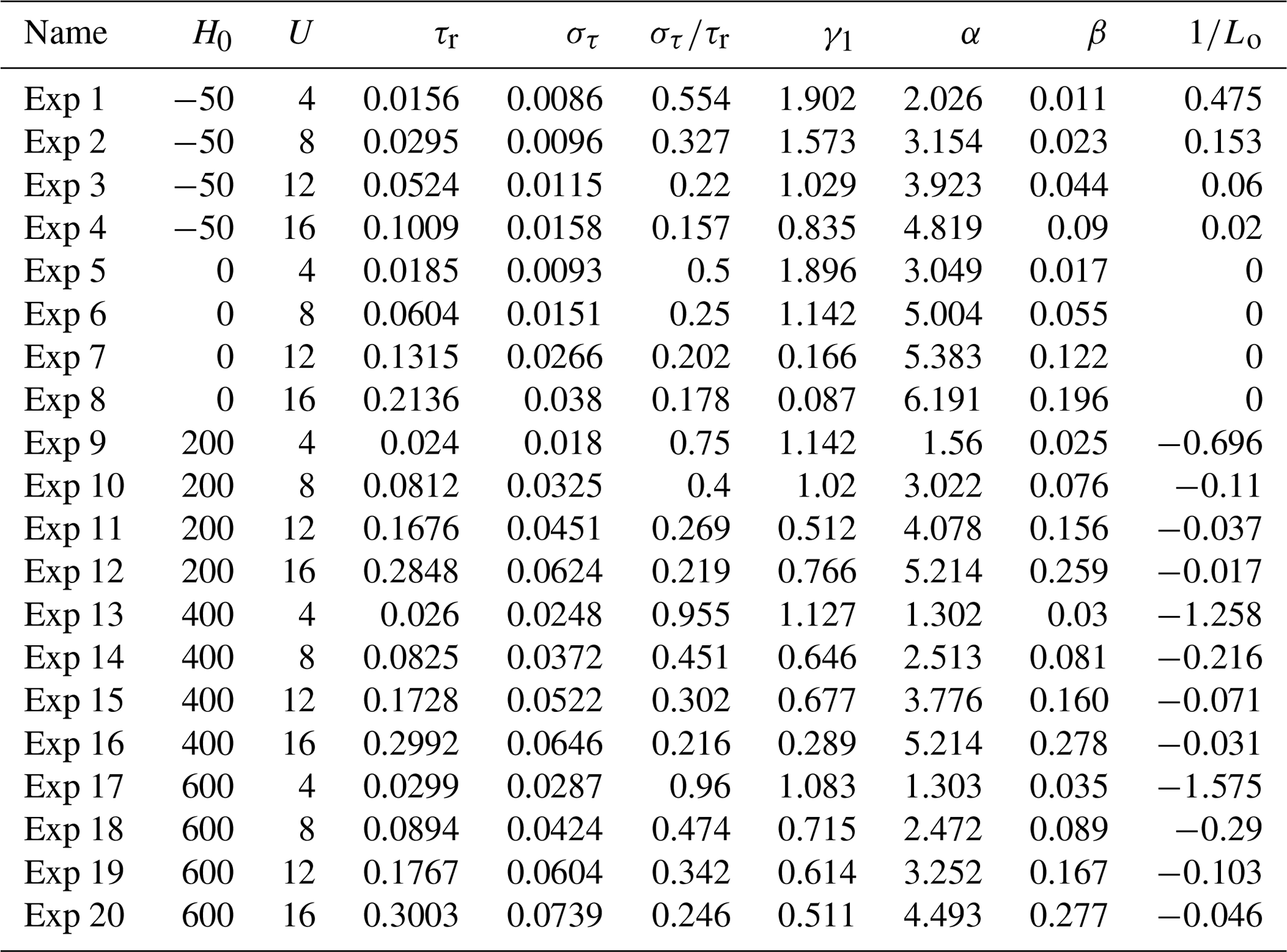
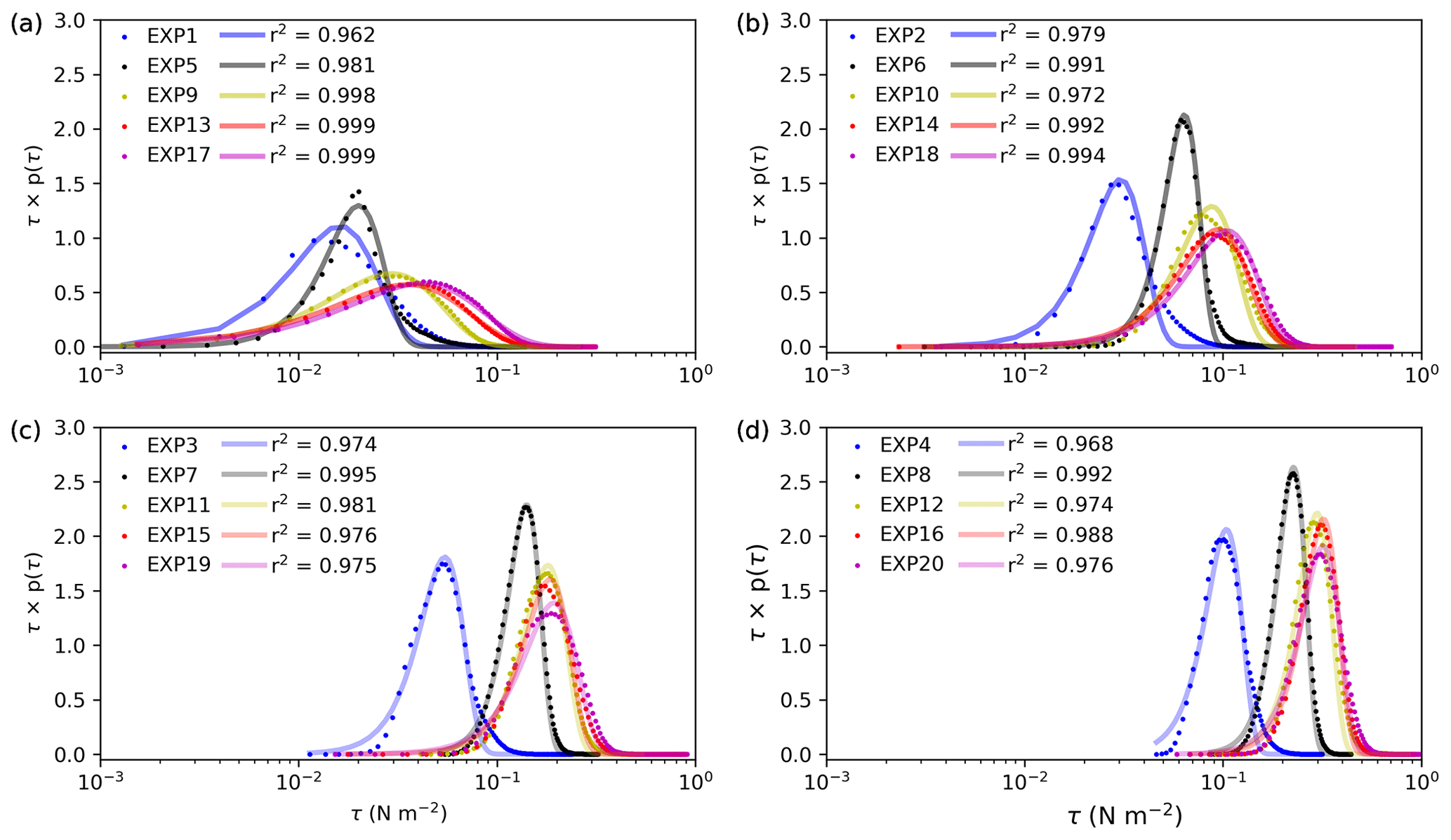
Figure 3Probability density functions derived from WRF-LES/D simulated surface shear stress τ (dots) and the corresponding fitted Weibull density functions (solid lines, r2 is the coefficients of determination) for different surface heat fluxes and different wind speeds: (a) U=4 m s−1, (b) U=8 m s−1, (c) U=12 m s−1, and (d) U=16 m s−1 with z0=0.153 mm.
The parameterization of surface shear stress has attracted intense interest; for example, Klose et al. (2014) reported that τ in unstable conditions is Weibull-distributed based on large-eddy simulations. Shao et al. (2020) found that p(τ) is skewed to small τ values (i.e., positively skewed) based on field observations. Li et al. (2020) suggested that τ in neutral conditions is Gauss-distributed based on a wind tunnel experiment. Colella and Keith (2003) explained that in turbulent shear flows, the nonlinear interaction between the eddies gives rise to a departure from Gaussian behavior. Our results show that the Gaussian approximation is inadequate in representing the skewed p(τ), especially for the conditions of strong turbulence intensity (e.g., unstable cases in Fig. 3a). Therefore, p(τ) here is approximated using a Weibull distribution, i.e.,
where α and β are the shape and scale parameters, respectively. The values of α and β for the numerical experiments Exp (1–20) are listed in Table 2. It can be seen that both α and β depend on wind speed and atmospheric stability. However, β is mainly determined by wind conditions when the wind is strong, while it is affected by ABL stability when the wind is weak. The behavior of α and β is shown in Fig. 4. is the absolute value of the reciprocal of the Obukhov length Lo, which can be calculated using
In both stable and unstable atmospheric conditions, analysis shows that the scale parameter α is related to ABL stability as the power of . Figure 4a shows that α decreases with the , satisfying Eq. (24) approximately. For neutral conditions, Lo goes to infinity, and Eq. (24) no longer applies. Therefore, the shape parameter obtained by the fitting was directly used for pdf reproduction for the neutral cases instead of the approximated α used for stable and unstable conditions. As Fig. 4b shows, the β parameter increases almost linearly with but can be best approximated using Eq. (25), with .
Using Eqs. (22)–(25), we can approximately describe the turbulent surface shear stress in non-neutral cases.
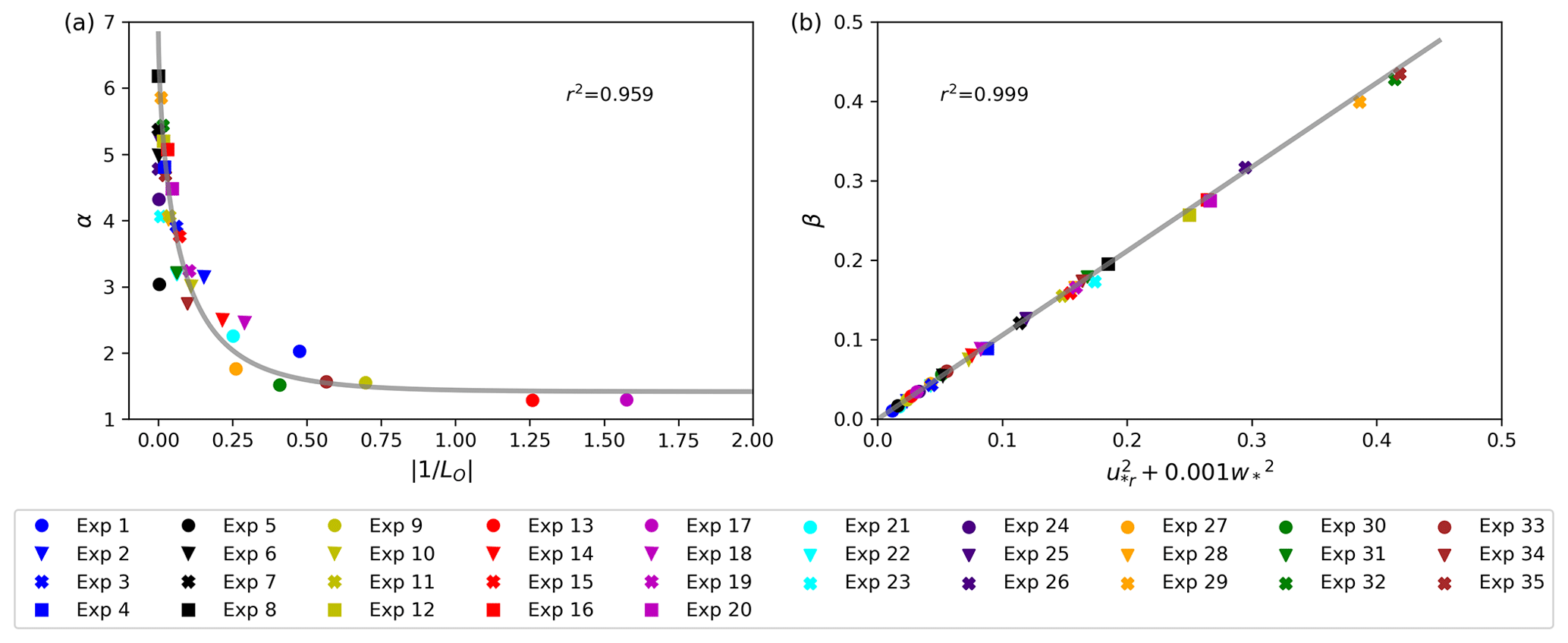
Figure 4(a) Dependency of the shape parameter α on for all numerical experiments Exp (1–35). (b) Dependency of scaling parameter β on for Exp (1–35).

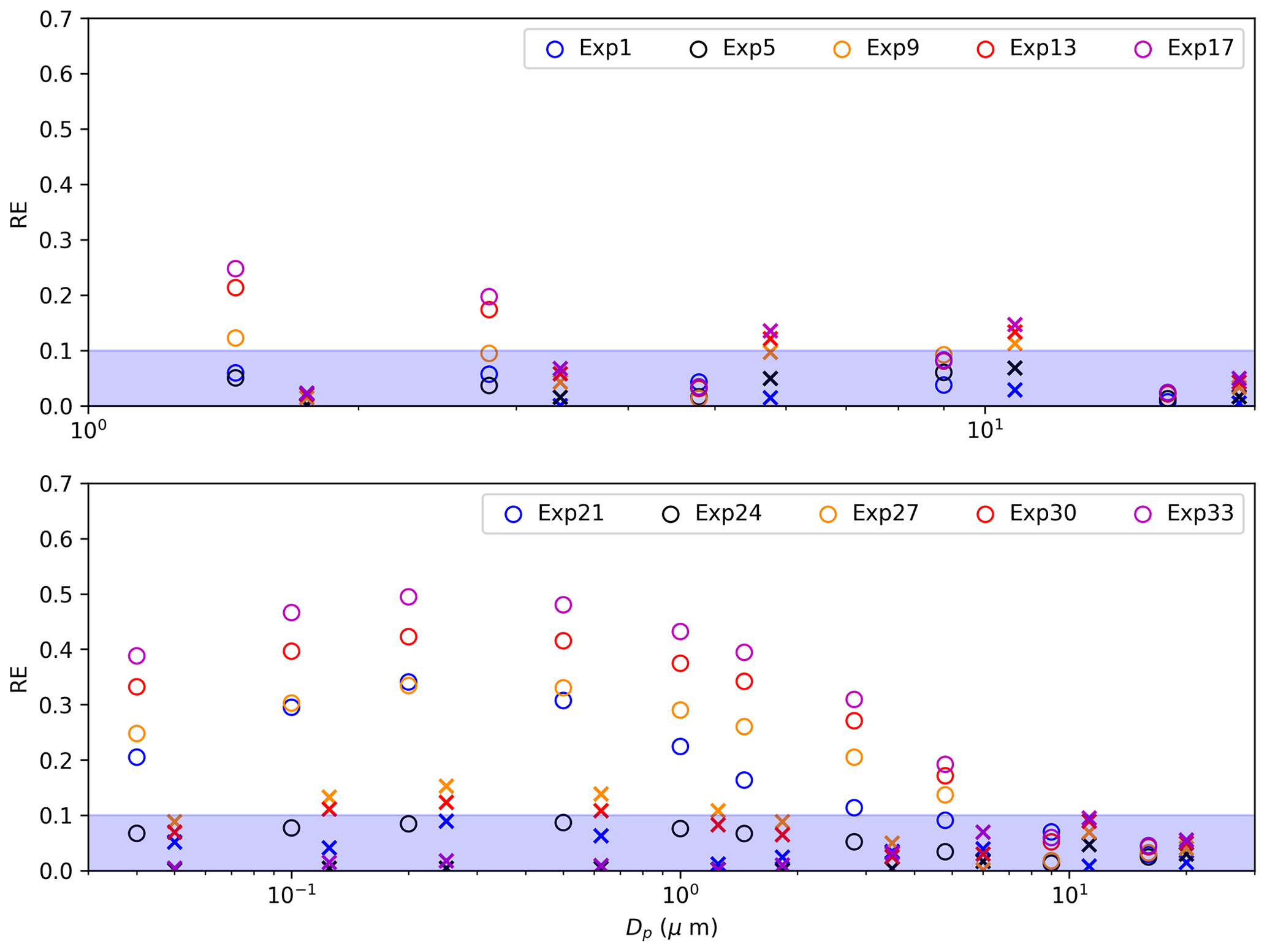
Figure 5(a) Validation of the simulated deposition velocity from WRF-LES/D (circles) by comparing with the observation data (crosses). (b) The comparison of the predicted result by ZS14 scheme (lines) with the simulated value (circles) of Exp (5, 9, 17) (left) and Exp (24, 27, 33) (right). (c) The comparison of the predicted result by the improved scheme (lines) with the simulated value (circles) of Exp (5, 9, 17) (left) and Exp (24, 27, 33) (right). (d) Comparison of relative error as a function of shear stress turbulence intensity (TI-S), estimated by ZS14 scheme (circles) and the improved scheme (crosses) for Exp (1–20) (left) and Exp (24, 27, 30, 33) (right).
3.2 Improvement to particle-deposition scheme
Figure 5a shows the performance of WRF-LES/D by comparing the simulated deposition velocity, Vd,LES, with wind tunnel experiments (Zhang and Shao, 2014) and field observation (Bergametti et al., 2018). The observed data are measured under neutral conditions and similar wind flow. As shown, the simulation results agree well with the observed data. On this basis, by further evaluating the performance of the ZS14 scheme, we found that the accuracy of the ZS14 scheme decreases with increasing instability. For example, Fig. 5b compares the deposition velocities of Exp (5, 9, 17) and Exp (24, 27, 33), Vd,LES, with those calculated by the ZS14 scheme using τr from the corresponding experiments, . It shows that under weak wind conditions, predicts the deposition well under neutral conditions and underestimates the deposition under convective conditions, especially for particles that are not dominated by molecular diffusion and gravity, and the underestimation increases with the atmospheric instability. To predict the deposition velocity more accurately for convective conditions, we need to account for the effect of shear stress fluctuations, i.e., the instantaneous shear stress distribution. Thus, the dry deposition scheme can be improved as
with p(τ) as given by Eqs. (22)–(25). As Fig. 5c shows, the improved scheme results Vd,τ and the simulation value Vd,LES show a remarkable congruence.
To make the comparison more clear, the relative errors (REs) of the predicted deposition velocity by the ZS14 scheme and improved scheme are compared with the WRF-LES/D simulation value and are calculated as below:
Analysis shows that the value of relative error (RE) depends on surface conditions, wind conditions, atmospheric stabilities, and particle sizes. It increases obviously with increased atmospheric instability under weak wind conditions, while it becomes less sensitive to stability when the wind is strong. Through the analysis, we find that the RE of the ZS14 scheme generally increases with the shear stress turbulence intensity, TI-S, and the value depends on particle size, as shown in Fig. 5d (left). Thus, we compared the RE of some different sized particles to investigate the particle in which size range is strongly affected (Fig. A2). The result shows that the RE first increases and then decreases with increasing particle size, and the particles with size normally in the range of 0.01 to 5 µm are strongly affected by turbulent shear stress, and p(τ) needs to be considered. After modification, the errors are limited to less than 10 % or approximately 10 %. For example, the relative error of Exp (17; i.e., U =4 m s−1 and H0=600 W m−2) for particles of 1.46 µm is reduced from ∼25 % to ∼3 %. The relative error of Exp (33; i.e., U =5.44 m s−1 and H0=600 W m−2) for particles of 0.5 µm is reduced from ∼50 % to ∼12 %.
To further analyze if the RE of ZS14 in unstable conditions is dominated by kinetic instability or dynamic instability, the Richardson number is calculated. Analysis shows that TI-S is positively correlated to gradient Richardson number Ri (Eq. A1). Under unstable conditions associated with strong vertical motion and weak winds, the RE of ZS14 increases with the increasing magnitude of Richardson number Ri (Fig. A3). The relationship between Ri and TI-S needs further study. Consequently, the results illustrate that the modified scheme Vd,τ tends to be more accurate than the unmodified scheme .
The present study was designed to determine the effect of ABL stability on particle deposition. For this purpose, the WRF-LES/D was used to model atmospheric-boundary-layer turbulence under the presence of atmospheric stability effects to recover statistics of shear stress variability. We then presented an improved particle-deposition scheme with the consideration of turbulent shear stress. While ABLS can broadly represent levels of atmospheric turbulence, its effect on particle deposition is wind-speed-dependent. Through a series of numerical experiments, we have shown the turbulent characteristics of particle-deposition velocity caused by the turbulent wind flow and pointed out the shortcomings of the ZS14 scheme in representing particle deposition under convective conditions. The relative error (RE) increases as the ABL instability increases for low wind conditions; i.e., the RE increases with shear stress turbulence intensity, especially for a certain size range of particles.
Since the dependency of particle deposition on micrometeorology is embedded in the application of the surface shear stress, we believe that the dependency of particle deposition on ABL stability is ultimately attributed to the statistical behavior of shear stress τ. Therefore, in this study, a model including the effects of surface shear fluctuations is proposed and validated by numerical experiments. Additionally, the fluctuations of surface shear caused by turbulence can be approximated with a Weibull distribution. The shape parameter decreases exponentially with the reciprocal of Monin–Obukhov length, and the scale parameter increases linearly with . After statistically revising the original scheme, an improved model is obtained. Using the modified model, the deposition velocity tends towards numerical experimental results.
The project is the first comprehensive investigation of the turbulent characteristics of particle deposition, and the findings will be of interest to improve the accuracy of particle-deposition predictions on regional or global scales. One source of weakness in this study is that the variation of τ may be changed by surface roughness and needs further study, as the roughness length does not fully reflect the effect of the surface topography on the turbulence structure. In spite of this limitation, the study adds to our understanding of the influence caused by ABLS on particle deposition.
Figure A1 shows the probability density distribution of surface shear stress for experiments (21–35); Fig. A2 shows the changing of relative error with particle size; Fig. A3 shows the variation of relative error (RE) of the ZS14 scheme (Eq. 10) and improved scheme (Eq. 26) with gradient Richardson number Ri.
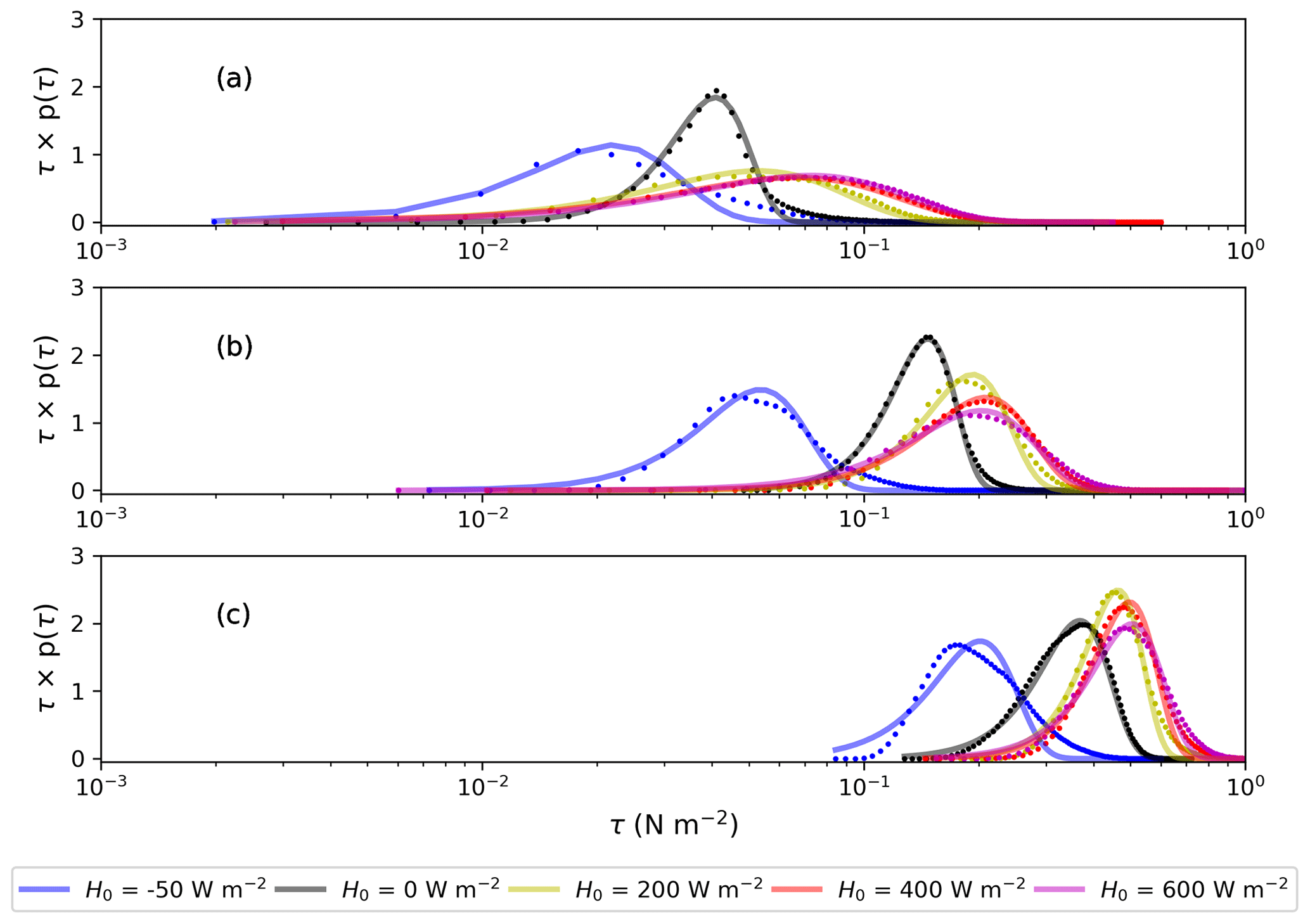
Figure A1Probability distributions of simulated surface shear stress τ (dots) and the corresponding fitted Weibull density distribution (solid lines) with different surface heat flux for different wind conditions: (a) U=5.44 m s−1, (b) U=10.87 m s−1, and (c) U=18.12 m s−1.
where z is the center height of the lowest layer, and is the potential temperature of the lowest layer.
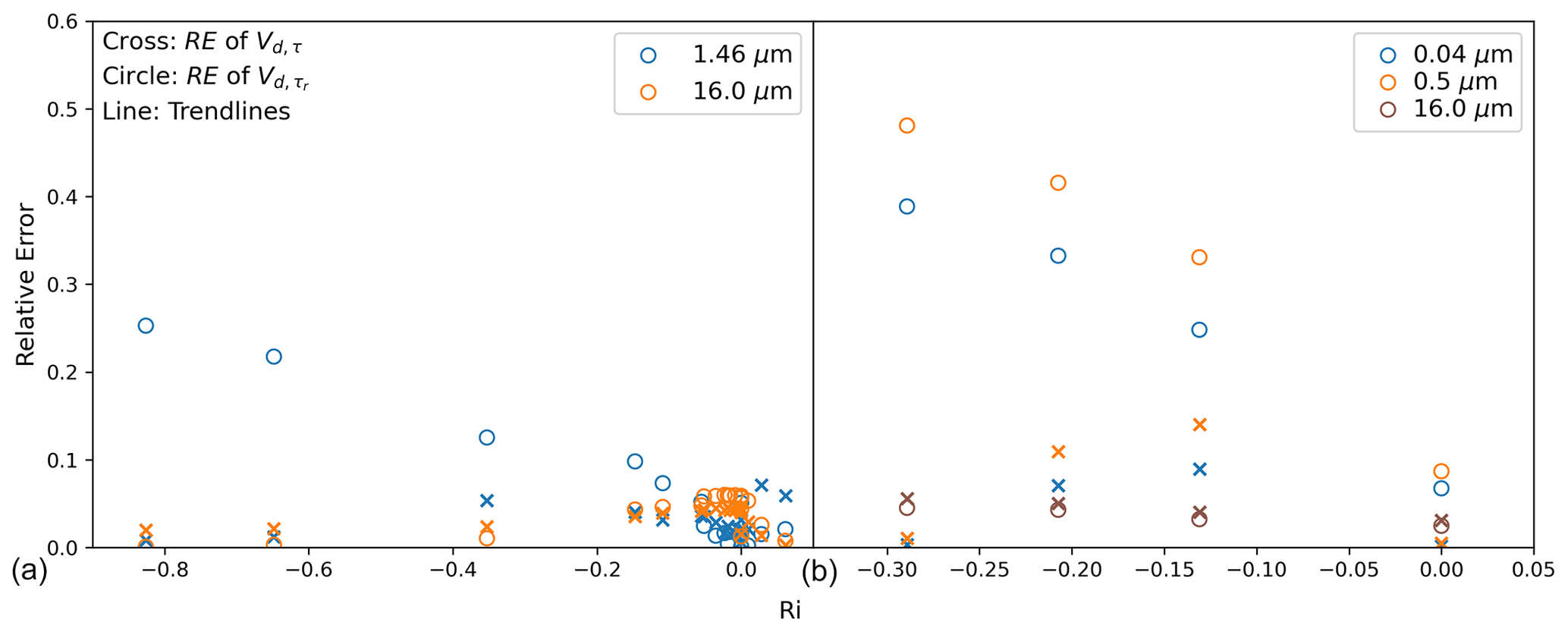
Figure A3Comparison of relative error as a function of Ri, estimated by ZS14 scheme (circles) and the improved scheme (crosses) for Exp (1–20) (a) and Exp (24, 27, 30, 33) (b).
The source code used in this study is the WRF-Chem version 3.7 in the LES mode coupled with a new deposition scheme. WRF-LES model can be downloaded at https://www2.mmm.ucar.edu/wrf/users/download/get_sources.html (WRF Users page, 2022). The code of the coupled deposition scheme and data set obtained by the simulation are available online at https://doi.org/10.5281/zenodo.6390432 (Yin et al., 2022).
XY, YP, and JZ were responsible for the formal analysis and methodology. XY and CJ were responsible for the data curation, software, validation, and visualization. YP, JZ, and NH were responsible for the supervision, project administration, and funding acquisition. XY was responsible for investigation and original draft preparation. XY, YP, JZ, and CJ were responsible for the review and editing of the paper.
The contact author has declared that neither they nor their co-authors have any competing interests.
Publisher's note: Copernicus Publications remains neutral with regard to jurisdictional claims in published maps and institutional affiliations.
This article is part of the special issue “Dust aerosol measurements, modeling and multidisciplinary effects (AMT/ACP inter-journal SI)”. It is not associated with a conference.
We thank the Second Tibetan Plateau Scientific Expedition and Research Program (grant no. 2019QZKK020611) the State Key Program of the National Natural Science Foundation of China (grant no. 41931179), the China Scholarship Council (201606180041), the Fundamental Research Funds for the Central Universities (grant no. lzujbky-2020-cd06), and the Major Science and Technology Project of Gansu Province (grant no. 21ZD4FA010).
This research has been supported by the Second Tibetan Plateau Scientific Expedition and Research Program (grant no. 2019QZKK020611), the State Key Program of the National Natural Science Foundation of China (grant no. 41931179), the China Scholarship Council (grant no. 201606180041), the Fundamental Research Funds for the Central Universities (grant no. lzujbky-2020-cd06), and the Major Science and Technology Project of Gansu Province (grant no. 21ZD4FA010).
This paper was edited by Stelios Kazadzis and reviewed by Gilles Bergametti and one anonymous referee.
Bergametti, G., Marticorena, B., Rajot, J. L., Foret, G., Alfaro, S. C., and Laurent, B.: Size-Resolved Dry Deposition Velocities of Dust Particles: In Situ Measurements and Parameterizations Testing, J. Geophys. Res.-Atmos., 123, 11080–11099, https://doi.org/10.1029/2018JD028964, 2018.
Chamberlain, A. C.: Aspects of travel and deposition of aerosol and vapour clouds, No. AERE-HP/R-1261, United Kingdom Atomic Energy Research Establishment, Harwell, Berks, England, 35 pp., UK, 1953.
Chamberlain, A. C.: Transport of Lycopodium spores and other small particles to rough surfaces, P. Roy. Soc. A.-Math. Phy., 296, 45–70, https://doi.org/10.1098/rspa.1967.0005, 1967.
Chen, S. H. and Dudhia, J.: Annual report: WRF physics, Air Force Weather Agency, Boulder, 1–38, 2000.
Colella, K. J. and Keith, W. L.: Measurements and scaling of wall shear stress fluctuations, Exp. Fluids, 34, 253–260, https://doi.org/10.1007/s00348-002-0552-2, 2003.
Connan, O., Pellerin, G., Maro, D., Damay, P., Hébert, D., Roupsard, P., Rozet, M., and Laguionie, P.: Dry deposition velocities of particles on grass: Field experimental data and comparison with models, J. Aerosol Sci., 126, 58–67, https://doi.org/10.1016/j.jaerosci.2018.08.004, 2018.
Csanady, G. T.: Turbulent Diffusion of Heavy Particles in the Atmosphere, J. Atmos. Sci., 20, 201–208, https://doi.org/10.1175/1520-0469(1964)021<0322:codohp>2.0.co;2, 1963.
Damay, P. E., Maro, D., Coppalle, A., Lamaud, E., Connan, O., Hébert, D., Talbaut, M., and Irvine, M.: Size-resolved eddy covariance measurements of fine particle vertical fluxes, J. Aerosol Sci., 40, 1050–1058, https://doi.org/10.1016/j.jaerosci.2009.09.010, 2009.
Deardorff, J. W.: Stratocumulus-capped mixed layers derived from a three-dimensional model, Bound.-Lay. Meteorol., 18, 495–527, https://doi.org/10.1007/BF00119502, 1980.
Droppo, J. G.: Improved Formulations for Air-Surface Exchanges Related to National Security Needs: Dry Deposition Models, Technical Report, Pacific Northwest National Lab (PNNL), Richland, WA, USA, 86 pp., https://doi.org/10.2172/890729, 2006.
Dudhia, J.: A multi-layer soil temperature model for MM5, Prepr. from Sixth PSU/NCAR Mesoscale Model Users' Work, 22–24 July 1996, Boulder, Colorado, 49–50, 1996.
Dupont, S., Bergametti, G., Marticorena, B., and Simoëns, S.: Modeling saltation intermittency, J. Geophys. Res.-Atmos., 118, 7109–7128, https://doi.org/10.1002/jgrd.50528, 2013.
Fowler, D., Pilegaard, K., Sutton, M. A., Ambus, P., Raivonen, M., Duyzer, J., Simpson, D., Fagerli, H., Fuzzi, S., Schjoerring, J. K., Granier, C., Neftel, A., Isaksen, I. S. A., Laj, P., Maione, M., Monks, P. S., Burkhardt, J., Daemmgen, U., Neirynck, J., Personne, E., Wichink-Kruit, R., Butterbach-Bahl, K., Flechard, C., Tuovinen, J. P., Coyle, M., Gerosa, G., Loubet, B., Altimir, N., Gruenhage, L., Ammann, C., Cieslik, S., Paoletti, E., Mikkelsen, T. N., Ro-Poulsen, H., Cellier, P., Cape, J. N., Horváth, L., Loreto, F., Niinemets, Ü., Palmer, P. I., Rinne, J., Misztal, P., Nemitz, E., Nilsson, D., Pryor, S., Gallagher, M. W., Vesala, T., Skiba, U., Brüggemann, N., Zechmeister-Boltenstern, S., Williams, J., O'Dowd, C., Facchini, M. C., de Leeuw, G., Flossman, A., Chaumerliac, N., and Erisman, J. W.: Atmospheric composition change: Ecosystems-Atmosphere interactions, Atmos. Environ., 43, 5193–5267, https://doi.org/10.1016/j.atmosenv.2009.07.068, 2009.
Gregory, P. H.: The dispersion of air-borne spores, T. Brit. Mycol. Soc., 28, 26–72, https://doi.org/10.1016/s0007-1536(45)80041-4, 1945.
Hicks, B. B., Saylor, R. D., and Baker, B. D.: Dry deposition of particles to canopies-A look back and the road forward, J. Geophys. Res., 121, 14691–14707, https://doi.org/10.1002/2015JD024742, 2016.
Kalitzin, G., Medic, G., and Templeton, J. A.: Wall modeling for LES of high Reynolds number channel flows: What turbulence information is retained?, Comput. Fluids, 37, 809–815, https://doi.org/10.1016/j.compfluid.2007.02.016, 2008.
Kawai, S. and Larsson, J.: Wall-modeling in large eddy simulation: Length scales, grid resolution, and accuracy, Phys. Fluids, 24, 015105, https://doi.org/10.1063/1.3678331, 2012.
Kind, R. J.: One-dimensional aeolian suspension above beds of loose particles-A new concentration-profile equation, Atmos. Environ., 26, 927–931, https://doi.org/10.1016/0960-1686(92)90250-O, 1992.
Klose, M. and Shao, Y.: Stochastic parameterization of dust emission and application to convective atmospheric conditions, Atmos. Chem. Phys., 12, 7309–7320, https://doi.org/10.5194/acp-12-7309-2012, 2012.
Klose, M. and Shao, Y.: Large-eddy simulation of turbulent dust emission, Aeolian Res., 8, 49–58, https://doi.org/10.1016/j.aeolia.2012.10.010, 2013.
Klose, M., Shao, Y., Li, X., Zhang, H., Ishizuka, M., Mikami, M., and Leys, J. F.: Further development of a parameterization for convective turbulent dust emission and evaluation based on field observations, J. Geophys. Res., 119, 10441–10457, https://doi.org/10.1002/2014JD021688, 2014.
Lamaud, E., Chapuis, A., Fontan, J., and Serie, E.: Measurements and parameterization of aerosol dry deposition in a semi-arid area, Atmos. Environ., 28, 2461–2471, https://doi.org/10.1016/1352-2310(94)90397-2, 1994.
Li, G., Zhang, J., Herrmann, H. J., Shao, Y., and Huang, N.: Study of Aerodynamic Grain Entrainment in Aeolian Transport, Geophys. Res. Lett., 47, e2019GL086574, https://doi.org/10.1029/2019GL086574, 2020.
Liu, D., Ishizuka, M., Mikami, M., and Shao, Y.: Turbulent characteristics of saltation and uncertainty of saltation model parameters, Atmos. Chem. Phys., 18, 7595–7606, https://doi.org/10.5194/acp-18-7595-2018, 2018.
Malcolm, L. P. and Raupach, M. R.: Measurements in an air settling tube of the terminal velocity distribution of soil material, J. Geophys. Res., 96, 15275–15286, 1991.
Moeng, C.-H., Dudhia, J., Klemp, J., and Sullivan, P.: Examining Two-Way Grid Nesting for Large Eddy Simulation of the PBL Using the WRF Model, Mon. Weather Rev., 135, 2295–2311, https://doi.org/10.1175/MWR3406.1, 2007.
Monahan, A. H.: The probability distribution of sea surface wind speeds. Part I: Theory and SeaWinds observations, J. Climate, 19, 497–520, https://doi.org/10.1175/JCLI3640.1, 2006.
Monin, A. S.: The Atmospheric Boundary Layer, Annu. Rev. Fluid Mech., 2, 225–250, https://doi.org/10.1146/annurev.fl.02.010170.001301, 1970.
Monin, A. S. and Obukhov, A. M.: Basic Laws of Turbulence Mixing in the Ground Layer of the Atmosphere, Tr. Akad. Nauk. SSSR Geophiz. Inst., 24, 163–187, 1954.
Monin, A. S., Yaglom, A. M., and Lumley, J. L.: Statistical Fluid Mechanics: Mechanics of Turbulence, Dover Publications, https://books.google.de/books?id=EtTyyI4_DvIC (last access: 11 May 2007), 2007.
Pellerin, G., Maro, D., Damay, P., Gehin, E., Connan, O., Laguionie, P., Hébert, D., Solier, L., Boulaud, D., Lamaud, E., and Charrier, X.: Aerosol particle dry deposition velocity above natural surfaces: Quantification according to the particles diameter, J. Aerosol Sci., 114, 107–117, https://doi.org/10.1016/j.jaerosci.2017.09.004, 2017.
Petroff, A. and Zhang, L.: Development and validation of a size-resolved particle dry deposition scheme for application in aerosol transport models, Geosci. Model Dev., 3, 753–769, https://doi.org/10.5194/gmd-3-753-2010, 2010.
Piomelli, U., Balaras, E., Squires, K. D., and Spalart, P. R.: Zonal approaches to wall-layer models for large-eddy simulations, 3rd Theoretical Fluid Mechanics Meeting, St Louis, Missouri, USA, 25 June 2002, 3083, https://doi.org/10.2514/6.2002-3083, 2002.
Pleim, J. E. and Xiu, A.: Development of a land surface model. Part II: Data assimilation, J. Appl. Meteorol., 42, 1811–1822, https://doi.org/10.1175/1520-0450(2003)042<1811:DOALSM>2.0.CO;2, 2003.
Rana, S., Anderson, W., and Day, M.: Turbulence-Based Model for Subthreshold Aeolian Saltation, Geophys. Res. Lett., 47, 1–9, https://doi.org/10.1029/2020GL088050, 2020.
Robinson, S. K.: Coherent motions in the turbulent boundary layer, Annu. Rev. Fluid Mech., 23, 601–639, https://doi.org/10.1146/annurev.fl.23.010191.003125, 1991.
Sehmel, G. A.: Particle and gas dry deposition: A review, Atmos. Environ., 14, 983–1011, https://doi.org/10.1016/0004-6981(80)90031-1, 1980.
Seinfeld, J. H. and Pandis, S. N.: Atmospheric Chemistry and Physics: From Air Pollution to Climate Change, , 2nd Edition, John Wiley & Sons, New York, 1152 pp., https://books.google.de/books?id=tZEpAQAAMAAJ (last access: 1 June 2016), 2006.
Seinfeld, J. H., Bretherton, C., Carslaw, K. S., Coe, H., DeMott, P. J., Dunlea, E. J., Feingold, G., Ghan, S., Guenther, A. B., Kahn, R., Kraucunas, I., Kreidenweis, S. M., Molina, M. J., Nenes, A., Penner, J. E., Prather, K. A., Ramanathan, V., Ramaswamy, V., Rasch, P. J., Ravishankara, A. R., Rosenfeld, D., Stephens, G., and Wood, R.: Improving our fundamental understanding of the role of aerosol-cloud interactions in the climate system, P. Natl. Acad. Sci. USA, 113, 5781–5790, https://doi.org/10.1073/PNAS.1514043113, 2016.
Shao, Y.: Simplification of a dust emission scheme and comparison with data, J. Geophys. Res.-Atmos., 109, 1–6, https://doi.org/10.1029/2003JD004372, 2004.
Shao, Y., Liu, S., Schween, J. H., and Crewell, S.: Large-Eddy Atmosphere-Land-Surface Modelling over Heterogeneous Surfaces: Model Development and Comparison with Measurements, Bound.-Lay. Meteorol., 148, 333–356, https://doi.org/10.1007/s10546-013-9823-0, 2013.
Shao, Y., Zhang, J., Ishizuka, M., Mikami, M., Leys, J., and Huang, N.: Dependency of particle size distribution at dust emission on friction velocity and atmospheric boundary-layer stability, Atmos. Chem. Phys., 20, 12939–12953, https://doi.org/10.5194/acp-20-12939-2020, 2020.
Skamarock, W. C., Klemp, J. B., Dudhi, J., Gill, D. O., Barker, D. M., Duda, M. G., Huang, X.-Y., Wang, W., and Powers, J. G.: A Description of the Advanced Research WRF Version 3, Tech. Rep., 113, https://doi.org/10.5065/D6DZ069T, 2008.
Slinn, S. A. and Slinn, W. G. N.: Predictions for particle deposition on natural waters, Atmos. Environ., 14, 1013–1016, https://doi.org/10.1016/0004-6981(80)90032-3, 1980.
Slinn, W. G. N.: Predictions for particle deposition to vegetative canopies, Atmos. Environ., 16, 1785–1794, https://doi.org/10.1016/0004-6981(82)90271-2, 1982.
Walcek, C. J., Brost, R. A., Chang, J. S., and Wesely, M. L.: SO2, sulfate and HNO3 deposition velocities computed using regional landuse and meteorological data, Atmos. Environ., 20, 949–964, https://doi.org/10.1016/0004-6981(86)90279-9, 1986.
Wesely, M. L., Cook, D. R., and Hart, R. L.: Fluxes of gases and particles above a deciduous forest in wintertime, Bound.-Lay. Meteorol., 27, 237–255, https://doi.org/10.1007/BF00125000, 1983.
Wesely, M. L., Cook, D. R., and Hart, R. L.: Measurements and parameterization of particulate sulfur dry deposition over grass., J. Geophys. Res., 90 2131–2143, https://doi.org/10.1029/jd090id01p02131, 1985.
WRF Users page: WRF Source Codes and Graphics Software Downloads [code], http://www2.mmm.ucar.edu/wrf/users/download/get_sources.html, last access: 11 January 2022.
Wyngaard, J. C.: Turbulence in the atmosphere, 1st edition, Cambridge University Press, Cambridge, 406 pp., https://doi.org/10.1017/CBO9780511840524, 2010.
Yang, Y. and Shao, Y.: A scheme for scalar exchange in the urban boundary layer, Bound.-Lay. Meteorol., 120, 111–132, https://doi.org/10.1007/s10546-005-9033-5, 2006.
Yin, X., Jiang, C., Shao, Y. P., Huang, N., and Zhang, J., Data download page: Simulation results obtained in the LES study of dust deposition on the desert surface, Zenodo [data set], https://doi.org/10.5281/zenodo.6390432, 2022.
Zhang, J. and Shao, Y.: A new parameterization of particle dry deposition over rough surfaces, Atmos. Chem. Phys., 14, 12429–12440, https://doi.org/10.5194/acp-14-12429-2014, 2014.
Zhang, L., Gong, S., Padro, J., and Barrie, L.: A size-segregated particle dry deposition scheme for an atmospheric aerosol module, Atmos. Environ., 35, 549–560, https://doi.org/10.1016/S1352-2310(00)00326-5, 2001.
Zheng, X., Jin, T., and Wang, P.: The Influence of Surface Stress Fluctuation on Saltation Sand Transport Around Threshold, J. Geophys. Res.-Earth, 125, e2019JF005246, https://doi.org/10.1029/2019JF005246, 2020.