the Creative Commons Attribution 4.0 License.
the Creative Commons Attribution 4.0 License.
 | 29 Mar 2022
Impacts of aerosol–photolysis interaction and aerosol–radiation feedback on surface-layer ozone in North China during multi-pollutant air pollution episodes
Hao Yang
Lei Chen
Hong Liao
Wenjie Wang
We examined the impacts of aerosol–radiation interactions, including the effects of aerosol–photolysis interaction (API) and aerosol–radiation feedback (ARF), on surface-layer ozone (O3) concentrations during four multi-pollutant air pollution episodes characterized by high O3 and PM2.5 levels during 28 July to 3 August 2014 (Episode1), 8–13 July 2015 (Episode2), 5–11 June 2016 (Episode3), and 28 June to 3 July 2017 (Episode4) in North China, by using the Weather Research and Forecasting with Chemistry (WRF-Chem) model embedded with an integrated process analysis scheme. Our results show that API and ARF reduced the daytime shortwave radiative fluxes at the surface by 92.4–102.9 W m−2 and increased daytime shortwave radiative fluxes in the atmosphere by 72.8–85.2 W m−2, as the values were averaged over the complex air pollution areas (CAPAs) in each of the four episodes. As a result, the stabilized atmosphere decreased the daytime planetary boundary layer height and 10 m wind speed by 129.0–249.0 m and 0.05–0.15 m s−1, respectively, in CAPAs in the four episodes. Aerosols were simulated to reduce the daytime near-surface photolysis rates of J[NO2] and J[O1D] by 1.8 × 10⁻³–2.0 × 10⁻³ and 5.7 × 10⁻⁶–6.4 × 10⁻⁶ s−1, respectively, in CAPAs in the four episodes. All of the four episodes show the same conclusion, which is that the reduction in O3 by API is larger than that by ARF. API (ARF) was simulated to change daytime surface-layer O3 concentrations by −8.5 ppb (parts per billion; −2.9 ppb), −10.3 ppb (−1.0 ppb), −9.1 ppb (−0.9 ppb), and −11.4 ppb (+0.7 ppb) in CAPAs of the four episodes, respectively. Process analysis indicated that the weakened O3 chemical production made the greatest contribution to API effect, while the reduced vertical mixing was the key process for ARF effect. Our conclusions suggest that future PM2.5 reductions may lead to O3 increases due to the weakened aerosol–radiation interactions, which should be considered in air quality planning.
- Article
(6107 KB) - Full-text XML
-
Supplement
(3220 KB) - BibTeX
- EndNote


The characteristics of air pollution in China during recent years have changed from a single pollutant (e.g. PM2.5, i.e. particulate matter with an aerodynamic equivalent diameter of 2.5 µm or less), to multiple pollutants (e.g. PM2.5 and ozone and O3; Zhao et al., 2018; Zhu et al., 2019), and the synchronous occurrence of high PM2.5 and O3 concentrations has been frequently observed, especially during the warm seasons (Dai et al., 2021; Qin et al., 2021). Qin et al. (2021) reported that the co-occurrence of PM2.5 and O3 pollution days (days with PM2.5 concentration > 75 µg m−3 and maximum daily 8 h average ozone concentration > 80 ppb; parts per billion) exceeded 324 d in eastern China during 2015–2019. Understanding complex air pollution is essential for making plans to improve air quality in China.
Aerosols can influence O3 by changing the meteorology through absorbing and scattering solar radiation (defined as aerosol–radiation feedback (ARF) in this work; Albrecht, 1989; Haywood and Boucher, 2000; Lohmann and Feichter, 2005), which influences the air quality by altering the chemical reactions, transport, and deposition of the pollutant (Gao et al., 2018; Qu et al., 2021; Xing et al., 2017; Zhang et al., 2018). Many studies have examined the feedback between aerosols and meteorology (Gao et al., 2015; M. Gao et al., 2016; Qiu et al., 2017; Chen et al., 2019; Zhu et al., 2021). For example, Gao et al. (2015) used the Weather Research and Forecasting with Chemistry (WRF-Chem) model to investigate the feedbacks between aerosols and meteorological variables over the North China Plain in January 2013 and pointed out that aerosols caused a decrease in surface temperature by 0.8–2.8 ∘C but an increase of 0.1–0.5 ∘C around 925 hPa. By using the same WRF-Chem model, Qiu et al. (2017) reported that the surface downward shortwave radiation and planetary boundary layer height (PBLH) were reduced by 54.6 W m−2 and 111.4 m, respectively, due to the aerosol direct radiative effect during 21–27 February 2014 in the North China Plain. Such aerosol-induced changes in meteorological fields are expected to influence O3 concentrations during multi-pollutant episodes with high concentrations of air pollutants.
Aerosols can also influence O3 by altering photolysis rates (defined as aerosol–photolysis interaction (API) in this work; Dickerson et al., 1997; Liao et al., 1999; Li et al., 2011; Lou et al., 2014). Dickerson et al. (1997) reported that the presence of pure scattering aerosol increased ground level ozone in the eastern United States by 20 to 45 ppb , while the presence of strongly absorbing aerosol reduced ground level ozone by up to 24 ppb. Wang et al. (2019) found that aerosols reduced the net ozone production rate by 25 % by reducing the photolysis frequencies during a comprehensive field observation in Beijing in August 2012. Such aerosol-induced changes in the photolysis rates are expected to influence O3 concentrations during multi-pollutant episodes with high concentrations of air pollutants.
Few previous studies have quantified the effects of ARF and API on O3 concentrations. Xing et al. (2017) applied a two-way online coupled WRF-CMAQ (Community Multi-scale Air Quality) model and reported that the combination of API and ARF reduced the surface daily maximum 1 h O3 (MDA1 O3) by up to 39 µg m−3 over China during January 2013. Qu et al. (2021) found, by using the UK Earth System Model (UKESM1), that ARF reduced the annual average surface O3 by 3.84 ppb (14.9 %) in the North China Plain during 2014. Gao et al. (2020) analysed the impacts of API on O3 by using the WRF-Chem model and reported that API reduced surface O3 by 10.6 ppb (19.0 %), 8.6 ppb (19.4 %), and 8.2 ppb (17.7 %) in Beijing, Tianjin, and Shijiazhuang, respectively, during October 2018. However, these previous studies mostly examined either ARF or API and did not examine their total and respective roles in O3 pollution in China. Furthermore, these previous studies lacked process understanding about the impacts of ARF and API on O3 pollution under the co-occurrence of PM2.5 and O3 pollution events.
The present study aims to quantify the respective/combined impacts of ARF and API on surface O3 concentrations by using the WRF-Chem model and to identify the prominent physical and/or chemical processes responsible for ARF and API effects by using an integrated process rate (IPR) analysis embedded in the WRF-Chem model. We carry out simulations and analyses on four multi-pollutant air pollution episodes (Episode1 is 28 July to 3 August 2014; Episode2 is 8–13 July 2015; Episode3 is 5–11 June 2016; Episode4 is 28 June to 3 July 2017) in North China with high O3 and PM2.5 levels (the daily mean PM2.5 and the maximum daily 8 h average O3 concentration are larger than 75 µg m−3 and 80 ppb, respectively). These episodes are selected because (1) these events with high concentrations of both PM2.5 and O3 are the major subjects of air pollution control, (2) high concentrations of both PM2.5 and O3 allow one to obtain the strongest signals of ARF and API, (3) the measurements of J[NO2] during 2014 and 2015 from the Peking University site (Wang et al., 2019) can help to constrain the simulated photolysis rates of NO2, and (4) selected events cover different years (2014 to 2017) during which the governmental Air Pollution Prevention and Control Action Plan was implemented (the changes in emissions and observed PM2.5 in the studied region during 2014–2017 are shown in Fig. S1 in the Supplement). We expect that the conclusions obtained from multiple episodes represent the general understanding of the impacts of ARF and API.
The model configuration, numerical experiments, observational data, and the integrated process rate analysis are described in Sect. 2. Section 3 shows the model evaluation. Results and discussions are presented in Sect. 4, and the conclusions are summarized in Sect. 5.
2.1 Model configuration
Version 3.7.1 of the online coupled Weather Research and Forecasting with Chemistry (WRF-Chem) model (Grell et al., 2005; Skamarock et al., 2008) is used in this study to explore the impacts of aerosol–radiation interactions on surface-layer O3 in North China. WRF-Chem can simulate gas-phase species and aerosols coupled with meteorological fields and has been widely used to investigate air pollution over North China (M. Gao et al., 2016; Gao et al., 2020; Wu et al., 2020). As shown in Fig. 1, we design two nested model domains with the number of grid points at 57 (west–east) × 41 (south–north) and 37 (west–east) × 43 (south–north) at 27 and 9 km horizontal resolutions, respectively. The parent domain centres at (39∘ N, 117∘ E). The model contains 29 vertical levels from the surface to 50 hPa, with 14 levels below 2 km for the full description of the vertical structure of planetary boundary layer (PBL).
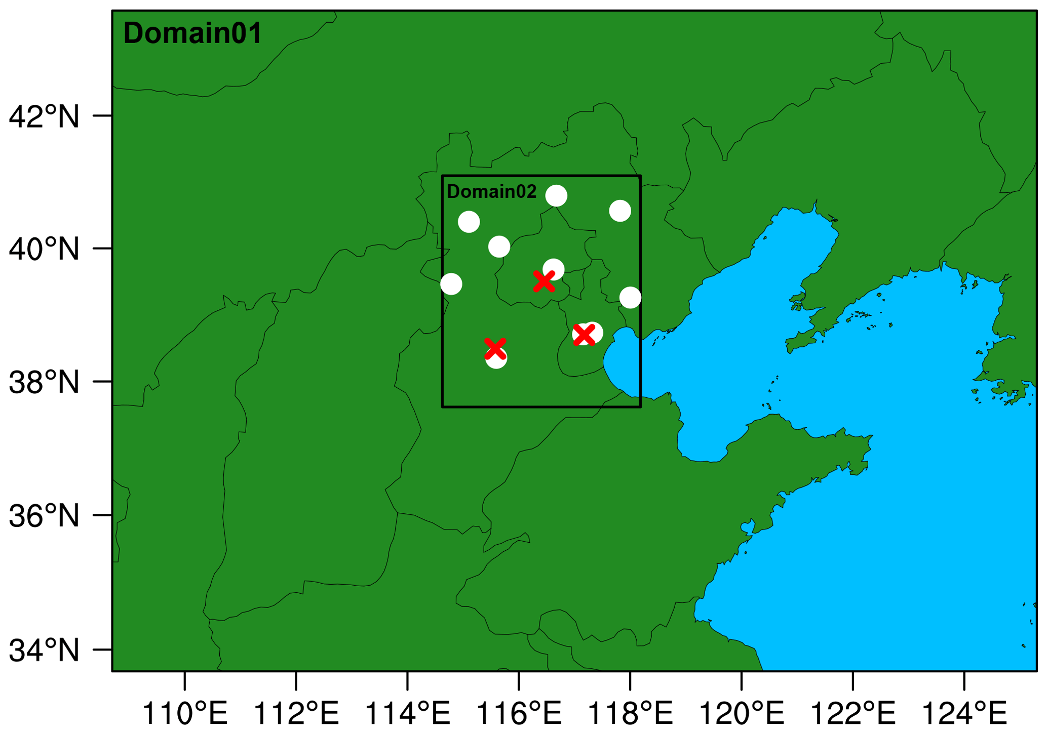
Figure 1Map of the two WRF-Chem modelling domains, with the locations of meteorological (white dots) and environmental (red crosses) observation sites used for model evaluation.
Table 1Physical parameterization options used in the simulation.
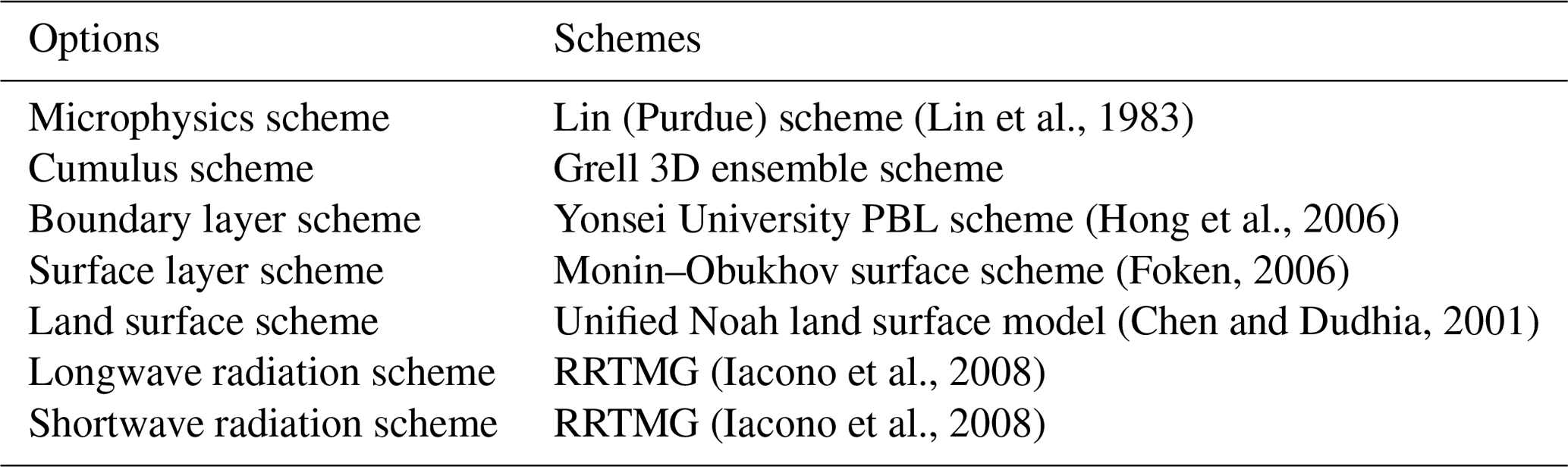
The Carbon Bond Mechanism Z (CBM-Z) is selected as the gas-phase chemical mechanism (Zaveri and Peters, 1999), and the full eight-bin MOSAIC (Model for Simulating Aerosol Interactions and Chemistry) module with aqueous chemistry is used to simulate aerosol evolution (Zaveri et al., 2008). The photolysis rates are calculated by the Fast-J scheme (Wild et al., 2000). Other major physical parameterizations used in this study are listed in Table 1.
The initial and boundary meteorological conditions are provided by the National Centers for Environmental Prediction (NCEP) Final (FNL) analysis data, with a spatial resolution of 1∘ × 1∘. In order to limit the model bias of simulated meteorological fields, the four-dimensional data assimilation (FDDA) is used with the nudging coefficient of 3.0 × 10⁻⁴ for wind, temperature, and humidity (no analysis nudging is applied for the inner domain; Lo et al., 2008; Otte, 2008). Chemical initial and boundary conditions are obtained from the Model for Ozone and Related chemical Tracers, version 4 (MOZART-4), forecasts (Emmons et al., 2010).
Anthropogenic emissions in these four episodes are taken from the Multi-resolution Emission Inventory for China (MEIC; http://www.meicmodel.org/, last access: 24 March 2022; M. Li et al., 2017). These emission inventories provide emissions of sulfur dioxide (SO2), nitrogen oxides (NOx), carbon monoxide (CO), non-methane volatile organic compounds (NMVOCs), carbon dioxide (CO2), ammonia (NH3), black carbon (BC), organic carbon (OC), PM10 (particulate matter with an aerodynamic diameter of 10 µm and less), and PM2.5. Emissions are aggregated from four sectors, including power generation, industry, residential, and transportation, with 0.25∘ × 0.25∘ spatial resolution. Biogenic emissions are calculated online by the Model of Emissions of Gases and Aerosols from Nature (MEGAN; Guenther et al., 2006).
2.2 Numerical experiments
To quantify the impacts of API and ARF on O3, the following three experiments have been conducted: (1) BASE – the base simulation coupled with the interactions between aerosol and radiation, which includes both impacts of API and ARF; (2) NOAPI – the same as the BASE case but the impact of API is turned off (aerosol optical properties are set to zero in the photolysis module), following Wu et al. (2020); and (3) NOALL – both the impacts of API and ARF are turned off (removing the mass of aerosol species when calculating aerosol optical properties in the optical module), following Qiu et al. (2017). The differences between BASE and NOAPI (i.e. BASE minus NOAPI) represent the impacts of API. The contributions from ARF can be obtained by comparing NOAPI and NOALL (i.e. NOAPI minus NOALL). The combined effects of API and ARF on O3 concentrations can be quantitatively evaluated by the differences between BASE and NOALL (i.e. BASE minus NOALL).
All the experiments in Episode1, Episode2, Episode3, and Episode4 are conducted from 26 July to 3 August 2014, 6–13 July 2015, 3–11 June 2016, and 26 June to 3 July 2017, respectively, with the first 40 h as the model spin-up in each case. Simulation results from the BASE cases of the four episodes are used to evaluate the model performance.
2.3 Observational data
Simulation results are compared with meteorological and chemical measurements. The surface-layer meteorological data (2 m temperature (T2), 2 m relative humidity (RH2), and 10 m wind speed (WS10)) with the temporal resolution of 3 h at 10 stations (Table S1 in the Supplement) are obtained from NOAA's National Climatic Data Center (https://www.ncei.noaa.gov/maps/hourly/, last access: 24 March 2022). The radiosonde data of temperature at 08:00 and 20:00 LST in Beijing (39.93∘ N, 116.28∘ E) are provided by the University of Wyoming (http://weather.uwyo.edu/, last access: 24 March 2022). Observed hourly concentrations of PM2.5 and O3 at 32 sites (Table S2) in North China are collected from the China National Environmental Monitoring Center (CNEMC). The photolysis rate of nitrogen dioxide (J[NO2]) measured at the Peking University site (39.99∘ N, 116.31∘ E) is also used to evaluate the model performance. More details about the measurement technique of J[NO2] can be found in Wang et al. (2019). The aerosol optical depth (AOD) at the Beijing site (39.98∘ N, 116.38∘ E) is provided by AERONET (level 2.0; http://aeronet.gsfc.nasa.gov/, last access: 24 March 2022). The AODs at 675 and 440 nm are used to derive the AOD at 550 nm to compare with the simulated ones.
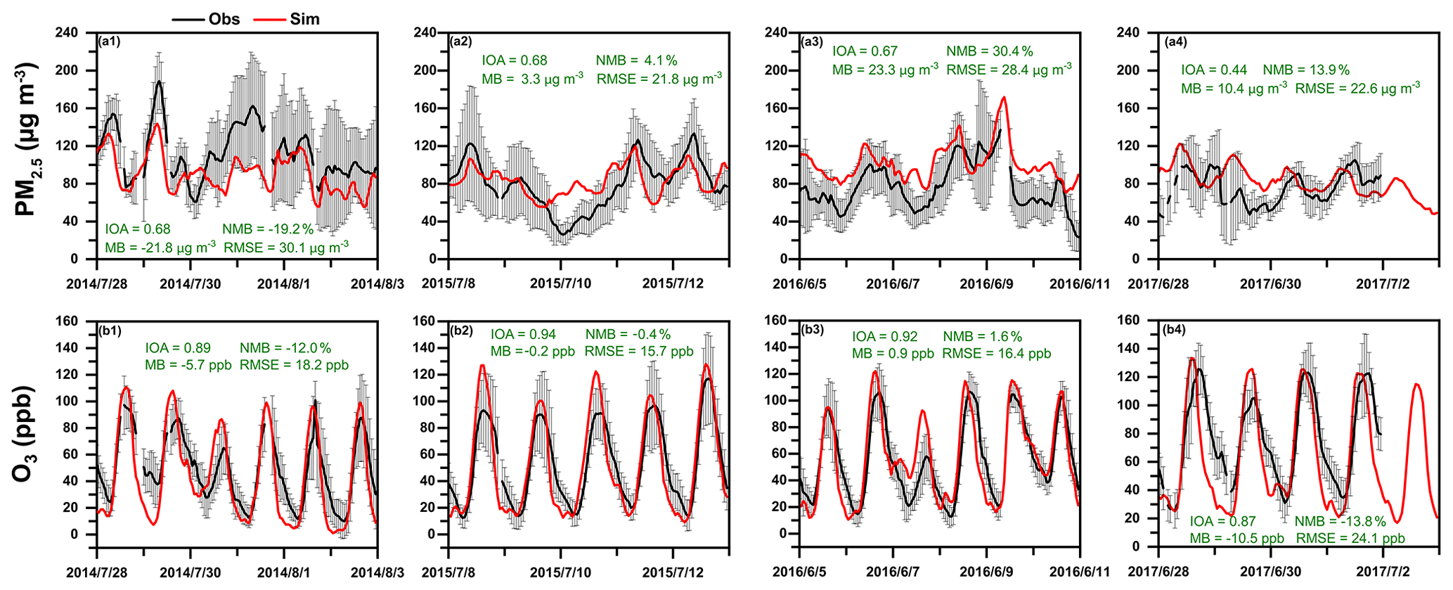
Figure 2Time series of observed (black) and simulated (red) hourly surface (a) PM2.5 and (b) O3 concentrations averaged over the 32 observation sites in Beijing, Tianjin, and Baoding during 28 July to 3 August 2014 (Episode1; a1 and b1), 8–13 July 2015 (Episode2; a2 and b2), 5–11 June 2016 (Episode3; a3 and b3), and 28 June to 3 July 2017 (Episode4; a4 and b4). The error bars represent the standard deviations. The calculated index of agreement (IOA), mean bias (MB), normalized mean bias (NMB), and root mean square error (RMSE) are also shown.
2.4 Integrated process rate analysis
Integrated process rate (IPR) analysis has been widely used to quantify the contributions of different processes to O3 variations (Goncalves et al., 2009; J. Gao et al., 2016; Gao et al., 2018; Tang et al., 2017). In this study, four physical/chemical processes are considered, including vertical mixing (VMIX), net chemical production (CHEM), horizontal advection (ADVH), and vertical advection (ADVZ). VMIX is initiated by turbulent process and closely related to PBL development, which influences O3 vertical gradients. CHEM represents the net O3 chemical production (chemical production minus chemical consumption). ADVH and ADVZ represent transport by winds (J. Gao et al., 2016). In this study, we define ADV as the sum of ADVH and ADVZ.
Reasonable representation of the observed meteorological and chemical variables by the WRF-Chem model can provide the foundation for evaluating the impacts of aerosols on surface-layer ozone concentrations. The model results presented in this section are taken from the BASE cases in the four episodes. The concentrations of air pollutants are averaged over the 32 observation sites in Beijing, Tianjin, and Baoding. To ensure the data quality, the mean value for each time is calculated only when concentrations are available at more than 16 sites, as done in J. D. Li et al. (2019).
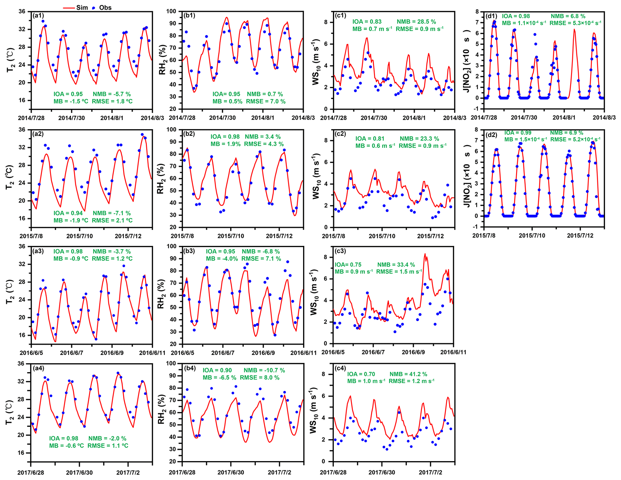
Figure 3Time series of 3 h observed (blue dots) and hourly simulated (red lines) (a) 2 m temperature (T2), (b) 2 m relative humidity (RH2), and (c) wind speed at 10 m (WS10), averaged over 10 meteorological observation stations, and the (d) surface photolysis rate of NO2 (J[NO2]) during 28 July to 3 August 2014 (Episode1; a1–d1), 8–13 July 2015 (Episode2; a2–d2), 5–11 June 2016 (Episode3; a3–c3), and 28 June to 3 July 2017 (Episode4; a4–c4). The calculated index of agreement (IOA), mean bias (MB), normalized mean bias (NMB), and root mean square error (RMSE) are also shown.
3.1 Chemical simulations
Figure 2 shows the temporal variations in observed and simulated PM2.5 and O3 concentrations over North China for the four episodes. As shown in Fig. 2, the temporal variations in observed PM2.5 can be well performed by the model with index of agreement (IOA) of 0.68, 0.68, 0.67, and 0.44 and the normalized mean bias (NMB) of −19.2 %, 4.1 %, 30.4 %, and 13.9 % during Episode1, Episode2, Episode3, and Episode4, respectively. The model also tracks the diurnal variation in O3 over the North China well, with IOA of 0.89, 0.94, 0.92, and 0.87 and NMB of −12.0 %, −0.4 %, 1.6 %, and −13.8 % for Episode1, Episode2, Episode3, and Episode4, respectively.
Figure S2 shows the correlation between observed and simulated AOD at 550 nm in Beijing. In the WRF-Chem model, the AODs at 550 nm are calculated by using the values at 400 and 600 nm, according to the Ångström exponent. Analysing Fig. S2, the model can reproduce the observed AOD with R of 0.7 and NMB of 7.9 %.
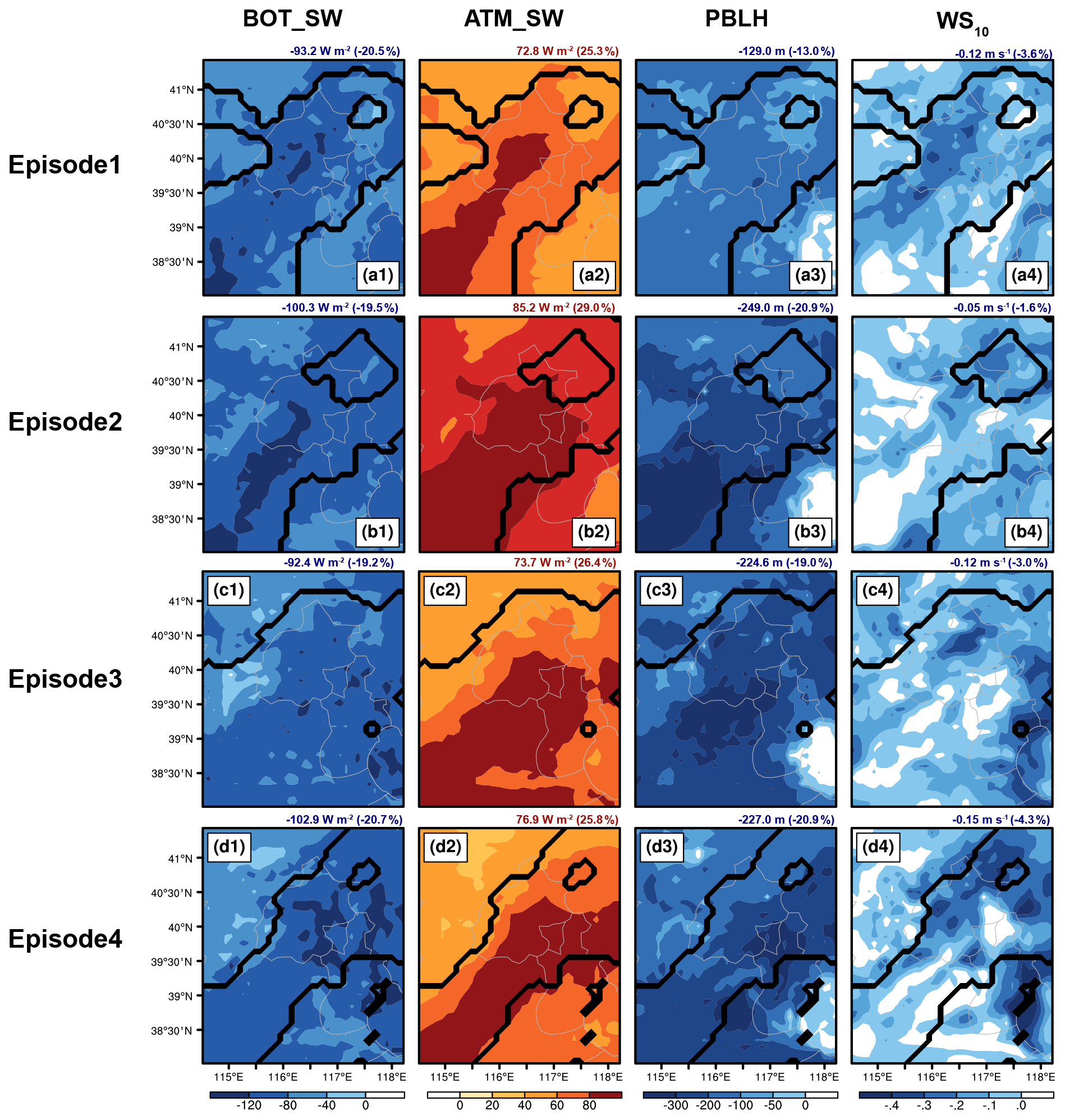
Figure 4The impacts of aerosol–radiation interactions on shortwave radiation at the surface (BOT_SW), shortwave radiation in the atmosphere (ATM_SW), PBL height (PBLH), and 10 m wind speed (WS10) in the daytime (08:00–17:00 LST) during 28 July to 3 August 2014 (Episode1), 8–13 July 2015 (Episode2), 5–11 June 2016 (Episode3), and 28 June to 3 July 2017 (Episode4). The regions sandwiched between two black lines are defined as the complex air pollution areas (CAPAs), where the mean daily PM2.5 and MDA8 O3 concentrations in the BASE case are larger than 75 µg m−3 and 80 ppb. The calculated changes (percentage changes) averaged over CAPAs are also shown at the top of each panel.
3.2 Meteorological simulations
Figure 3 shows the time series of observed and simulated T2, RH2, WS10, and J[NO2] during the four episodes. The observed T2, RH2, and WS10 are averaged over the 10 meteorological observation stations, and the J[NO2] are measured at Peking University. Most of the monitored J[NO2] in Episode3 and Episode4 are unavailable, so the comparison of J[NO2] in Episode3 and Episode4 is not shown. Generally, the model can depict the temporal variations in T2 fairly well, with IOA of 0.94–0.98 and the mean bias (MB) of −1.9 to −0.6 ∘C. For RH2, the IOA and MB are 0.90–0.98 and −6.5 % to 1.9 %, respectively. Although WRF-Chem model overestimates WS10 with the MB of 0.6–1.0 m s−1, the IOA for WS10 is 0.70–0.83, and the root mean square error (RMSE) is 0.9–1.5 m s−1, which is smaller than the threshold of the model performance criteria (2 m s−1) proposed by Emery et al. (2001). The positive bias in wind speed has also been reproduced in other studies (Zhang et al., 2010; Gao et al., 2015; Liao et al., 2015; Qiu et al., 2017). The predicted J[NO2] agrees well with the observations with IOA of 0.98–0.99 and NMB of 6.8 %–6.9 %. We also conduct comparisons of observed and simulated temperature profiles at 08:00 and 20:00 LST in Beijing during the four episodes (Fig. S3). The vertical profiles of observed temperature can be well captured by the model in these four complex air pollution episodes. Generally, the WRF-Chem model can reasonably reproduce the temporal variations in observed meteorological parameters.
We examine the impacts of aerosol–radiation interactions on O3 concentrations with a special focus on the complex air pollution areas (CAPAs; Fig. S4) in the four episodes, where the daily mean simulated PM2.5 and MDA8 (maximum daily 8 h average) O3 concentrations are larger than 75 µg m−3 and 80 ppb, respectively, based on the National Ambient Air Quality Standards (http://www.mee.gov.cn, last access: 24 March 2022).
4.1 Impacts of aerosol–radiation interactions on meteorology
Figure 4 shows the impacts of aerosol–radiation interactions on shortwave radiation at the surface (BOT_SW), shortwave radiation in the atmosphere (ATM_SW), PBLH, and WS10 during the daytime (08:00–17:00 LST) from Episode1 to Episode4. Analysing the results of the interactions between aerosol and radiation (the combined impacts of API and ARF), BOT_SW is decreased over the entire simulated domain in the four episodes with the decreases of 93.2 W m−2 (20.5 %), 100.3 W m−2 (19.5 %), 92.4 W m−2 (19.2 %), and 102.9 W m−2 (20.7 %) over CAPAs, respectively. Contrary to the changes in BOT_SW, ATM_SW is increased significantly in the four episodes, with the increases of 72.8 W m−2 (25.3 %), 85.2 W m−2 (29.0 %), 73.7 W m−2 (26.4 %), and 76.9 W m−2 (25.8 %) over CAPAs, respectively. The decreased BOT_SW perturbs the near-surface energy flux, which weakens convection and suppresses the development of PBL (Z. Li et al., 2017). The mean PBLHs over CAPAs are decreased by 129.0 m (13.0 %), 249.0 m (20.9 %), 224.6 m (19.0 %), and 227.0 m (20.9 %), respectively. WS10 exhibits overall reductions over CAPAs and is calculated to decrease by 0.12 m s−1 (3.6 %), 0.05 m s−1 (1.6 %), 0.12 m s−1 (3.0 %), and 0.15 m s−1 (4.3 %) for the four episodes, respectively. We also examine the changed meteorological variables caused by API and ARF, respectively. As shown in Figs. S5 and S6, API has little impact on meteorological variables, which means the major contributor to the meteorology variability is ARF.

Figure 5Spatial distributions of (a) simulated surface-layer PM2.5 concentrations in BASE cases and the changes in surface (b) J[NO2] and (c) J[O1D] due to aerosol–radiation interactions in the daytime (08:00–17:00 LST) during 28 July to 3 August 2014 (Episode1), 8–13 July 2015 (Episode2), 5–11 June 2016 (Episode3), and 28 June to 3 July 2017 (Episode4). The calculated values (percentage changes) averaged over CAPAs are also shown at the top of each panel.
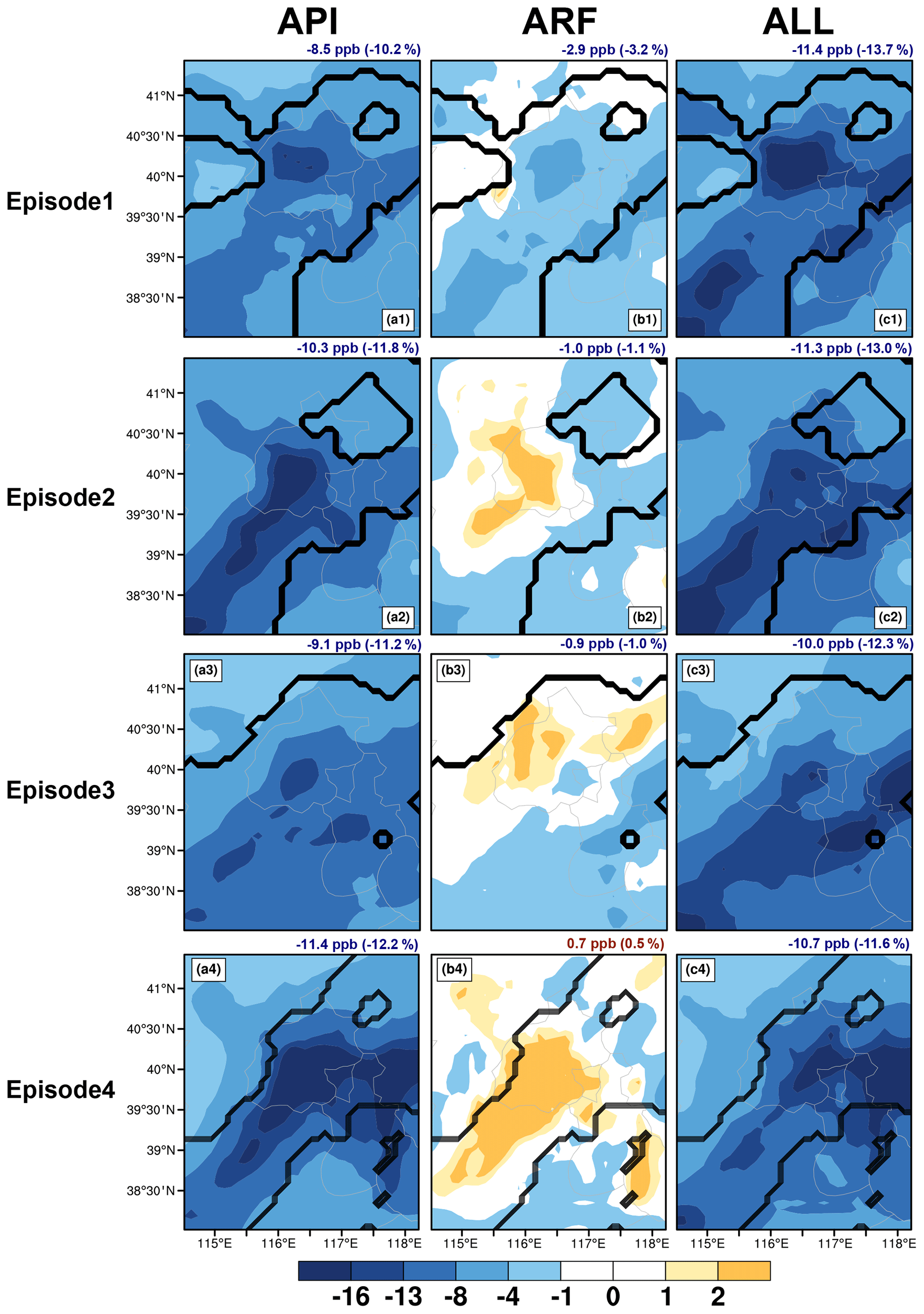
Figure 6The changes in surface-layer ozone due to (a) aerosol–photolysis interaction (API), (b) aerosol–radiation feedback (ARF), and (c) the combined effects (ALL; defined as API+ARF) in the daytime (08:00–17:00 LST) during 28 July to 3 August 2014 (Episode1), 8–13 July 2015 (Episode2), 5–11 June 2016 (Episode3), and 28 June to 3 July 2017 (Episode4). The changes (percentage changes) in O3 concentrations caused by API, ARF, and ALL, averaged over CAPAs, are also shown at the top of each panel.
4.2 Impacts of aerosol–radiation interactions on photolysis
Figure 5 shows the spatial distributions of mean daytime surface-layer PM2.5 concentrations simulated by the BASE cases and the changes in J[NO2] and J[O1D] due to aerosol–radiation interactions from Episode1 to Episode4. When the combined impacts (API and ARF) are considered, J[NO2] and J[O1D] are decreased over the entire domain in the four episodes, and the spatial patterns of changed J[NO2] and J[O1D] are similar to that of simulated PM2.5. Analysing the four simulated episodes, the surface J[NO2] averaged over CAPAs is decreased by 1.8 × 10⁻³ s−1 (40.5 %), 2.0 × 10⁻³ s−1 (36.8 %), 1.8 × 10⁻³ s−1 (36.0 %), and 2.0 × 10⁻³ s−1 (38.0 %), respectively. The decreased surface J[O1D] over CAPAs is 6.1 × 10⁻⁶ s−1 (48.8 %), 6.3 × 10⁻⁶ s−1 (41.4 %), 5.7 × 10⁻⁶ s−1 (44.6 %), and 6.4 × 10⁻⁶ s−1 (46.9 %), respectively. Figure S7 exhibits the impacts of API and ARF on surface J[NO2] and J[O1D]. Conclusions can be summarized that J[NO2] and J[O1D] are significantly modified by API and little affected by ARF.
4.3 Impacts of aerosol–radiation interactions on O3
Figure 6 shows the changes in surface-layer O3 due to API, ARF, and the combined effects (denoted as ALL) from Episode1 to Episode4. As shown in Fig. 6a1–a4, API alone leads to overall surface O3 decreases over the entire domain, with average reductions of 8.5 ppb (10.2 %), 10.3 ppb (11.8 %), 9.1 ppb (11.2 %), and 11.4 ppb (12.2 %) over CAPAs in the four episodes, respectively. The changes can be explained by the substantially diminished UV radiation due to aerosol loading, which significantly weakens the efficiency of photochemical reactions and restrains O3 formation. However, the decreased surface O3 concentrations due to ARF are only 2.9 ppb (3.2 %; Fig. 6b1), 1.0 ppb (1.1 %; Fig. 6b2) and 0.9 ppb (1.0 %; Fig. 6b3) for the Episode1 to Episode3 but ARF increased surface O3 concentrations by 0.7 ppb (0.5 %; Fig. 6b4) during Episode4, which was caused by the enhancement of chemical production (Fig. S10 and Sect. 4.4). All the episodes show same conclusion in that the reduction in O3 by API is larger than that by ARF. Figure 6c1–c4 presents the combined effects of API and ARF. Generally, aerosol–radiation interactions decrease the surface O3 concentrations by 11.4 ppb (13.7 %), 11.3 ppb (13.0 %), 10.0 ppb (12.3 %), and 10.7 ppb (11.6 %) averaged over CAPAs in the four episodes, respectively.
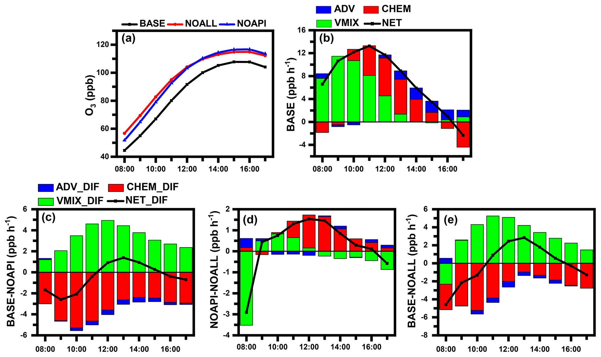
Figure 7Temporal evolution characteristics of aerosol–radiation interactions on O3 averaged over the four episodes. (a) Diurnal variations in simulated surface O3 concentrations in BASE (black dotted line), NOAPI (blue dotted line), and NOALL (red dotted line) cases over CAPAs. (b) The hourly surface O3 changes induced by each physical/chemical process, using the IPR analysis method in BASE case, are shown. (c–e) Changes in hourly surface O3 process contributions caused by API (BASE minus NOAPI), ARF (NOAPI minus NOALL), and ALL (BASE minus NOALL) over CAPAs during the daytime (08:00–17:00 LST) are shown. The black lines with squares denote the net contribution of all processes (NET; defined as VMIX+CHEM+ADV). Differences in each process contribution are denoted as VMIX_DIF, CHEM_DIF, ADV_DIF, and NET_DIF.
4.4 Influencing mechanism of aerosol–radiation interactions on O3
Figure 7a shows mean results of the four episodes (Episode1, Episode2, Episode3, and Episode4) in diurnal variations of simulated daytime surface-layer O3 concentrations from the BASE, NOAPI, and NOALL cases averaged over CAPAs. All of the experiments (BASE, NOAPI, and NOALL) present O3 increases from 08:00 LST. It is shown that the simulated O3 concentrations in the BASE case increase more slowly than that in the NOAPI and NOALL cases. To explain the underlying mechanisms of API and ARF impacts on O3, we quantify the variations in contributions of different processes (ADV, CHEM, and VMIX) to O3 by using the IPR analysis.
Figure 7b shows hourly surface O3 changes induced by each physical/chemical process (i.e. ADV, CHEM, and VMIX) in the BASE case averaged from Episode1 to Episode4. The significant positive contribution to the hourly variation in O3 is contributed by VMIX, and the contribution reaches the maximum at about 09:00 LST, since VMIX increases the surface O3 concentrations by transporting O3 from aloft (where O3 concentrations are high) to the surface layer (Tang et al., 2017; Xing et al., 2017; Gao et al., 2018). The CHEM process makes negative contributions at around 09:00 and 16:00 LST, which means that the chemical consumption of O3 is stronger than the chemical production. At noon, the net chemical contribution turns positive due to stronger solar UV radiation. The contribution from all the processes (NET, which is the sum of VMIX, CHEM, and ADV) to a O3 variation is peaked at noon and then becomes weakened. After sunset (17:00 LST), the NET contribution turns negative over CAPAs, leading to a O3 decrease.
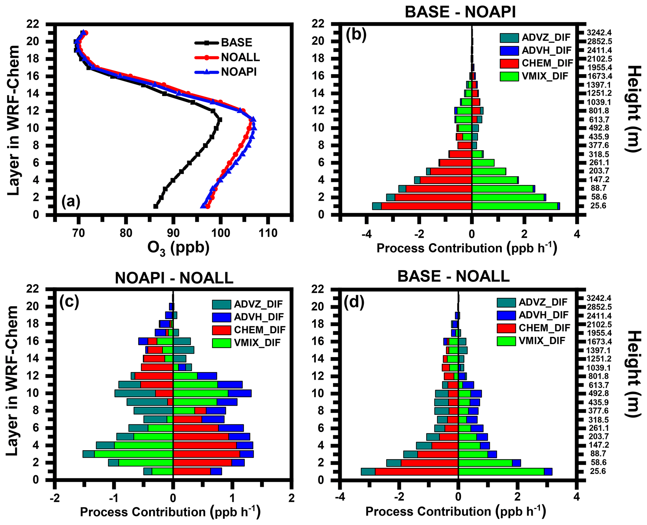
Figure 8The impacts of aerosol–radiation interactions on vertical O3 averaged over the four episodes. (a) Vertical profiles of simulated O3 concentrations in BASE (black dotted line), NOAPI (blue dotted line), and NOALL (red dotted line) cases over CAPAs. (b–d) Changes in O3 budget due to API, ARF, and ALL over CAPAs during the daytime (08:00–17:00 LST). Differences in each process contribution are denoted by ADVZ_DIF, ADVH_DIF, CHEM_DIF, and VMIX_DIF.
Figure 7c shows the changes in the hourly process contributions caused by API averaged from Episode1 to Episode4. The chemical production of O3 is suppressed significantly due to aerosol impacts on photolysis rates. The weakened O3 chemical production decreases the contribution from CHEM and results in a negative value of CHEM_DIF (−3.44 ppb h−1). In contrast to CHEM_DIF, the contribution from changed VMIX (VMIX_DIF) to the O3 concentration due to API is always positive, and the mean value is +3.26 ppb h−1. The positive change in VMIX due to API may be associated with the different vertical gradient of O3 between the BASE and NOAPI cases (Gao et al., 2020), as shown in Fig. 8a. The impact of API on ADV process is relatively small (−0.26 ppb h−1). NET_DIF, namely the sum of VMIX_DIF, CHEM_DIF, and ADV_DIF, indicates the differences in hourly O3 changes caused by API. As shown in Fig. 7c, NET_DIF is almost negative during the daytime over CAPAs, with the mean value of −0.44 ppb h−1. This is because the decreases in CHEM and ADV are larger than the increases in VMIX caused by API; the O3 decrease is mainly attributed to the significantly decreased contribution from CHEM. The maximum difference in O3 between the BASE and NOAPI appears at 11:00 LST, with a value of −12.5 ppb (Fig. 7a).
Figure 7d shows the impacts of ARF on each physical/chemical process contribution to the hourly O3 variation averaged from Episode1 to Episode4. At 08:00 LST, the change in VMIX due to ARF is large, with a value of −3.5 ppb h−1, resulting in a net negative variation with all processes considered. The decrease in O3 reaches the maximum with the value of 5.0 ppb at around 08:00 LST over CAPAs (Fig. 7a). During 09:00 to 16:00 LST, the positive VMIX_DIF (mean value of +0.10 ppb h−1) or the positive CHEM_DIF (mean value of +0.75 ppb h−1) is the major process leading to the positive NET_DIF. The positive VMIX_DIF is related to the evolution in the boundary layer during the daytime. The ratio is calculated to classify sensitivity regimes and to indicate the possible O3 responses to changes in volatile organic compounds (VOCs) and/or NOx concentrations. O3 production is VOC limited if the ratio is less than 4 and is NOx limited if the ratio is larger than 15 (Edson et al., 2017; K. Li et al., 2017). The ratio of ranges around 4–15 and indicates a transitional regime, where ozone is nearly equally sensitive to both species (Sillman, 1999). As shown in Fig. S8a–h, O3 is mainly formed under the VOC limited conditions and the transition regimes in CAPAs. As shown in Fig. S8i–l and m–p, both the surface concentrations of VOCs and NOx are increased when the impacts of ARF are considered. Thus, the contribution of CHEM in NOAPI is larger than that in NOALL.
When both impacts of API and ARF are considered, the variation pattern of the difference in hourly process contribution shown in Fig. 7e is similar to that in Fig. 7c, which indicates that API is the dominant factor to surface-layer O3 reduction.
Figure 8 presents the vertical profiles of simulated daytime O3 concentrations in three cases (BASE, NOAPI, and NOALL), and the differences in contributions from each physical/chemical process to hourly O3 variations caused by API, ARF, and the combined effects averaged over CAPAs from Episode1 to Episode4. As shown in Fig. 8a, the O3 concentration is lower in BASE than that in other two scenarios (NOAPI and NOALL), especially at the lower 12 levels (below 801.8 m), owing to the impacts of aerosols (API and/or ARF).
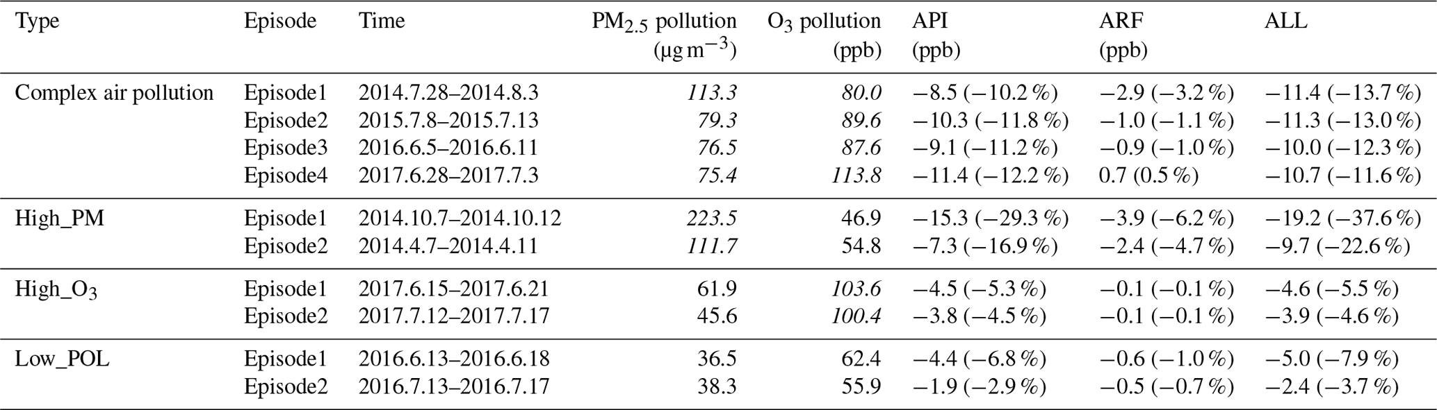
Table 2Detailed information of the analysed episodes, including the impacts of API, ARF, and ALL on O3 concentrations under different air pollution conditions. The numbers in italics indicate the concentrations exceeded the Class II limit of the National Ambient Air Quality Standards of China. The numbers in parentheses indicate the percentage changes in the O3 concentration.
The changes in each process contribution caused by API are presented in Fig. 8b. The contribution from CHEM_DIF is −2.1 ppb h−1 for the first seven layers (from 25.6 to 318.5 m). Conversely, the contribution from VMIX_DIF shows a positive value under the 318.5 m (between the first layer to the seventh layer), with the mean value of +1.8 ppb h−1. The positive variation in VMIX due to API may be associated with the different vertical gradient of O3 between BASE and NOAPI again. The contributions of changed advection (ADVH_DIF and ADVZ_DIF) are relatively small, with mean values of +0.03 and −0.18 ppb h−1 below the first seven layers, which may result from the small impact of API on the wind field (Fig. S6a4 to d4). The net difference is a negative value (−0.45 ppb h−1), and API leads to a O3 reduction not only near the surface but also aloft.
Figure 8c shows the differences in O3 budget due to ARF. When the ARF is considered, the vertical turbulence is weakened and the development of the PBL is inhibited, which makes VMIX_DIF negative at the lower seven layers (below the 318.5 m), with a mean value of −0.69 ppb h−1, but the variation in CHEM caused by ARF is positive, with a mean value of +0.86 ppb h−1. The enhanced O3 precursors due to ARF can promote the chemical production of O3 (Tie et al., 2009; Gao et al., 2018). The changes in ADVZ and ADVH (ADVZ_DIF and ADVH_DIF) caused by ARF are associated with the variations in the wind field. When ARF is considered, the horizontal wind speed is decreased (Fig. S9a), which makes ADVH_DIF positive at the lower 12 layers, with a mean value of +0.30 ppb h−1. However, ADVZ_DIF is negative at these layers, with a mean value of −0.26 ppb h−1, because aerosol radiative effects decrease the transport of O3 from the upper to lower layers (Fig. S9b).
In Fig. 8d, the pattern and magnitude of the differences in process contributions between BASE and NOALL are similar to those caused by API, indicating the dominate contributor of API on O3 changes. The impacts of API on O3 both near the surface and aloft are greater than those of ARF.
Figures S10 and S11 detail the influencing mechanism of aerosol–radiation interactions on O3 in each episode. Similar variation characteristics can be found among the four episodes as the mean situation (discussed above), with the larger impacts of API on O3 both near the surface and aloft than those of ARF, indicating that the role of API is much larger than that of ARF during all the simulated episodes.
4.5 Discussions
We presented above the results from our simulations of multi-pollutant air pollution episodes. In order to make the conclusion more general, we carried out simulations for three additional air pollution conditions, i.e. (1) PM2.5 pollution alone (High_PM, with daily mean PM2.5 concentration larger than 75 µg m−3), (2) O3 pollution alone (High_O3, with the maximum daily 8 h average O3 concentration larger than 80 ppb), and (3) neither PM2.5 nor O3 exceeded air quality standard (Low_POL, with daily mean PM2.5 and the maximum daily 8 h average O3 concentrations smaller than 75 µg m−3 and 80 ppb, respectively). For each condition of air pollution, we examined two episodes.
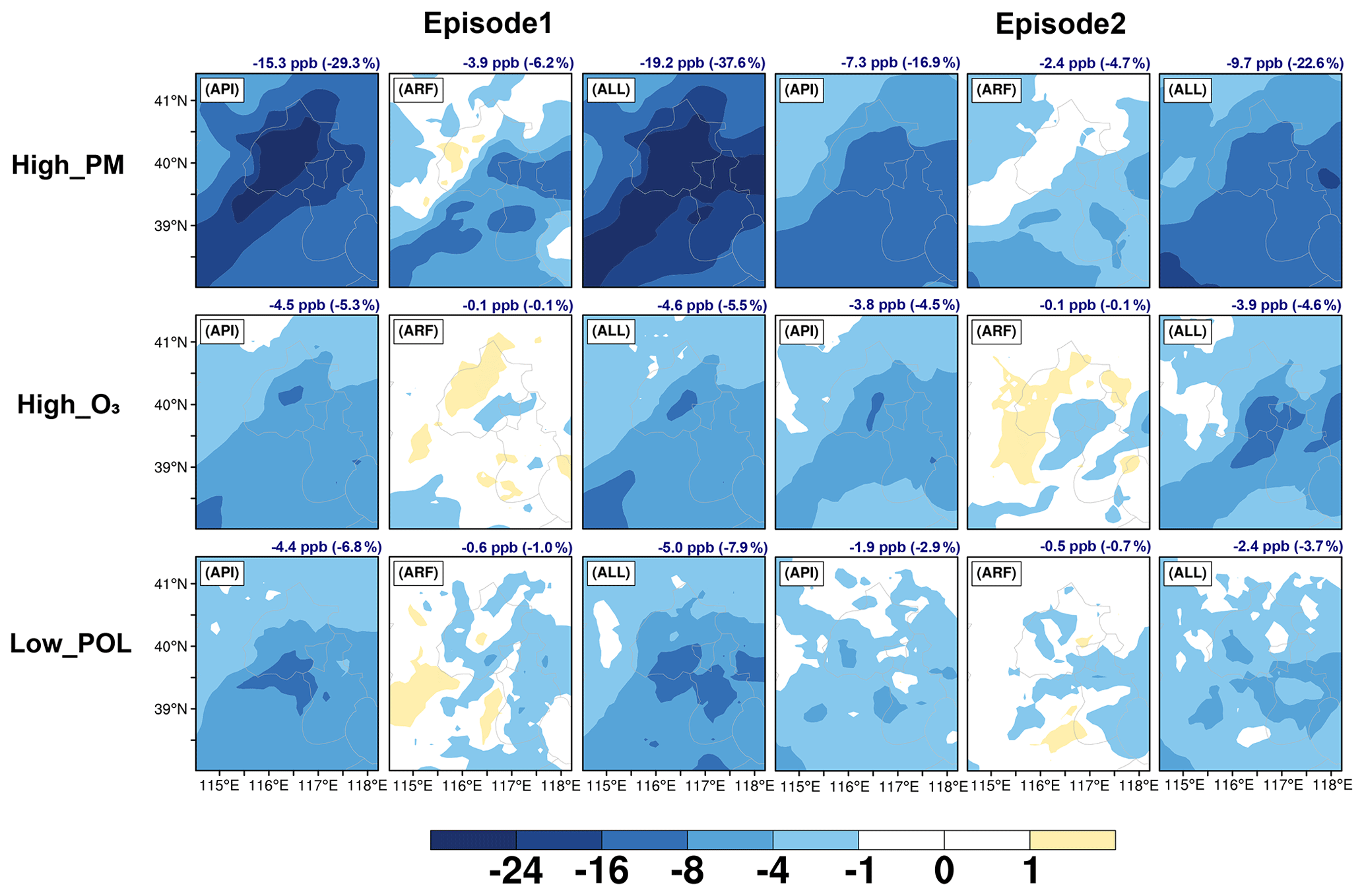
Figure 9The changes in surface-layer O3 due to aerosol–photolysis interaction (API), aerosol–radiation feedback (ARF), and the combined effects (ALL; API+ARF) in the daytime (08:00–17:00 LST) of 7–12 October 2014 (High_PM_Episode1), 7–11 April 2014 (High_PM_Episode2), 13–18 June 2016 (Low_POL_Episode1), 13–17 July 2016 (Low_POL_Episode2), 15–21 June 2017 (High_O3_Episode1), and 12–17 July 2017 (High_O3_Episode2). The changes (percentage changes) in O3 concentrations caused by API, ARF, and ALL, averaged over the entire simulated domain, are also shown at the top of each panel.
Figures S12 and S13 show the temporal variations in observed and simulated PM2.5 and O3 concentrations during 7–12 October 2014 (High_PM_Episode1), 7–11 April 2014 (High_PM_Episode2), 15–21 June 2017 (High_O3_Episode1), 12–17 July 2017 (High_O3_Episode2), 13–18 June 2016 (Low_POL_Episode1), and 13–17 July 2016 (Low_POL_Episode2). The temporal variations in observed PM2.5 can be well captured by the model, with IOAs of 0.63, 0.82, 0.56, 0.42, 0.76, and 0.54 and NMBs of 7.4 %, 20.3 %, −21.7 %, −25.9 %, 14.7 %, and −29.3 % during High_PM_Episode1, High_PM_Episode2, High_O3_Episode1, High_O3_Episode2, Low_POL_Episode1, and Low_POL_Episode2, respectively. The model also simulates the diurnal variation in O3 over the North China well, with IOAs of 0.87, 0.80, 0.87, 0.90, 0.84, and 0.86 and NMBs of −9.4 %, −29.5 %, −15.2 %, −9.4 %, 11.6 %, and 18.0 % in these six episodes, respectively.
Figure 9 shows changes in daytime surface-layer O3 due to API, ARF, and the combined effects (denoted as ALL) of High_PM_Episode1, High_PM_Episode2, High_O3_Episode1, High_O3_Episode2, Low_POL_Episode1, and Low_POL_Episode2. As summarized in Table 2, all the simulations confirm the same conclusion, which is that the reduction in O3 by API is larger than that by ARF. Averaged over the entire domain, the percentage reductions in O3 by API and ARF are, respectively, 29.3 % and 6.2 % in High_PM_Episode1, 16.9 % and 4.7 % in High_PM_Episode2, 5.3 % and 0.1 % in High_O3_Episode1, 4.5 % and 0.1 % in High_O3_Episode2, 6.8 % and 1.0 % in Low_POL_Episode1, and 2.9 % and 0.7 % in Low_POL_Episode2. It is worth noting that the percentage reductions in O3 from both API and ARF in High_PM episodes are 1.6–3.2 times the impacts in the complex episodes, while the impacts in cases of Low_POL and High_O3 are 0.3–0.7 times the impacts of complex episodes.
In this study, the fully coupled regional chemistry transport model WRF-Chem is applied to investigate the impacts of aerosol–radiation interactions, including the impacts of aerosol–photolysis interaction (API) and the impacts of aerosol–radiation feedback (ARF), on O3 during summertime complex air pollution episodes during 28 July to 3 August 2014 (Episode1), 8–13 July 2015 (Episode2), 5–11 June 2016 (Episode3), and 28 June to 3 July 2017 (Episode4). In total, three sensitivity experiments are designed to quantify the respective and combined impacts from API and ARF. Generally, the spatiotemporal distributions of the observed pollutant concentrations and meteorological parameters can be captured fairly well by the model, with an index of agreement of 0.44–0.94 for pollutant concentrations and 0.70–0.99 for meteorological parameters.
Sensitivity experiments show that aerosol–radiation interactions decrease BOT_SW, WS10, PBLH, J[NO2], and J[O1D] by 92.4–102.9 W m−2, 0.05–0.15 m s−1, 129.0–249.0 m, 1.8 × 10⁻³ –2.0 × 10⁻³ s−1, and 5.7 × 10⁻⁶ –6.4 × 10⁻⁶ s−1 over CAPAs and increase ATM_SW by 72.8–85.2 W m−2, respectively. The changed meteorological variables and weakened photochemistry reaction further reduce surface-layer O3 concentrations by 10.0–11.4 ppb, with relative changes of 74.6 %–106.5 % by API and of −6.5 % to 25.4 % by ARF.
We further examine the influencing mechanism of aerosol–radiation interactions on O3 by using integrated process rate analysis. API can directly affect O3 by reducing the photochemistry reactions within the lower several hundred metres and, therefore, amplify the O3 vertical gradient, which promotes the vertical mixing of O3. The reduced photochemistry reactions of O3 weaken the chemical contribution and reduce the surface O3 concentrations, even though the enhanced vertical mixing can partly counteract the reduction. ARF affects O3 concentrations indirectly through the changed meteorological variables, e.g. the decreased PBLH. The suppressed PBL can weaken the vertical mixing of O3 by turbulence. Generally, the impacts of API on O3 both near the surface and aloft are greater than those of ARF, indicating the dominant role of API on O3 reduction related to aerosol–radiation interactions.
This study provides a detailed understanding of aerosol impacts on O3 through aerosol–radiation interactions (including both API and ARF), with the general conclusion summarized as follows: when the impacts of aerosol–radiation interactions are considered, the changed meteorological variables and weakened photochemistry reaction can change surface-layer O3 concentrations during the warm season, and the API is the dominant factor for O3 reduction. The results can also imply that future PM2.5 reductions may lead to O3 increases due to weakened aerosol–radiation interactions. A recent study emphasized the need for controlling VOC emissions to mitigate O3 pollution (K. Li et al., 2019a). Therefore, tighter controls of O3 precursors (especially VOC emissions) are needed to counteract future O3 increases caused by weakened aerosol–radiation interactions.
There are some limitations in this work. (1) In the current Carbon Bond Mechanism Z (CBM-Z) and MOSAIC schemes, the formation of SOA (secondary organic aerosol) is not included (Gao et al., 2015; Chen et al., 2019). The absence of SOA can underestimate the impacts of API and ARF on O3. Meanwhile, the lack of SOA may lead to weaker heterogeneous reactions and result in higher O3 concentrations (K. Li et al., 2019b). The net effect of the two processes will be discussed and quantified in our future study. (2) The CNEMC network was built in 2013. Before 2013, the national observations of PM2.5 and O3 concentrations were not available, which makes it difficult to select the time and location of complex air pollution events and to evaluate the model results. Based on observation data, we were mainly focused on impacts of ARF and API on surface O3 for complex air pollution episodes from 2014 to 2017. Additional simulations of High_PM, High_O3, and Low_POL support the conclusion obtained from the complex air pollution episodes that the reduction in O3 by API is larger than that by ARF.
The observed hourly surface concentrations of air pollutants are derived from the China National Environmental Monitoring Center (https://air.cnemc.cn:18007/, CNEMC, 2022). The observed surface meteorological data are obtained from NOAA's National Climatic Data Center (https://www.ncei.noaa.gov/maps/hourly/, National Centers for Environmental Information, 2022). The radiosonde data are provided by the University of Wyoming (http://weather.uwyo.edu/upperair/sounding.html, University of Wyoming, 2022). The photolysis rates of nitrogen dioxide in Beijing are provided by Xin Li (li_xin@pku.edu.cn). The aerosol optical depth in Beijing is obtained from the AERONET level 2.0 data collection (http://aeronet.gsfc.nasa.gov/; NASA, 2022). The simulation results can be accessed by contacting Lei Chen (chenlei@nuist.edu.cn) and Hong Liao (hongliao@nuist.edu.cn).
The supplement related to this article is available online at: https://doi.org/10.5194/acp-22-4101-2022-supplement.
HY, LC, and HL conceived the study and designed the experiments. HY and LC performed the simulations and carried out the data analysis. JZ, WW, and XL provided useful comments on the paper. HY, LC, and HL prepared the paper, with contributions from all co-authors.
The contact author has declared that neither they nor their co-authors have any competing interests.
Publisher's note: Copernicus Publications remains neutral with regard to jurisdictional claims in published maps and institutional affiliations.
We acknowledge the computing resources from the university–industry collaborative education programme between the Ministry of Education and Huawei.
This research has been supported by National Natural Science Foundation of China (grant nos. 42021004, 91744311, and 42007195), the Meteorological Soft Science Program of China Meteorological Administration (grant no. 2021ZZXM46), and the Postgraduate Research and Practice Innovation Program of Jiangsu Province (grant no. KYCX21_1014).
This paper was edited by Jason West and reviewed by two anonymous referees.
Albrecht, B. A.: Aerosols, cloud microphysics, and fractional cloudiness, Science, 245, 1227–1230, 1989.
Chen, F. and Dudhia, J.: Coupling an Advanced Land Surface – Hydrology Model with the Penn State – NCAR MM5 Modeling System. Part I: Model Implementation and Sensitivity, Mon. Weather Rev., 129, 569–585, 2001.
Chen, L., Zhu, J., Liao, H., Gao, Y., Qiu, Y., Zhang, M., Liu, Z., Li, N., and Wang, Y.: Assessing the formation and evolution mechanisms of severe haze pollution in the Beijing–Tianjin–Hebei region using process analysis, Atmos. Chem. Phys., 19, 10845–10864, https://doi.org/10.5194/acp-19-10845-2019, 2019.
China National Environmental Monitoring Centre (CNEMC): Air pollutants dataset in China, CNEMC [data set], https://air.cnemc.cn:18007/, last access: 25 March 2022.
Dai, H., Zhu, J., Liao, H., Li, J., Liang, M., Yang, Y., and Yue, X.: Co-occurrence of ozone and PM2.5 pollution in the Yangtze River Delta over 2013–2019: Spatiotemporal distribution and meteorological conditions, Atmos. Res., 249, 105363, https://doi.org/10.1016/j.atmosres.2020.105363, 2021.
Dickerson, R. R., Kondragunta, S., Stenchikov, G., Civerolo, K. L., Doddridge, B. G., and Holben, B. N.: The impact of aerosols on solar ultraviolet radiation and photochemical smog, Science, 278, 827–830, https://doi.org/10.1126/science.278.5339.827, 1997.
Edson, C. T., Ivan, H.-P., and Alberto, M.: Use of combined observational- and model-derived photochemical indicators to assess the O3-NOx-VOC System sensitivity in urban areas, Atmosphere, 8, 22, https://doi.org/10.3390/atmos8020022, 2017.
Emery, C., Tai, E., and Yarwood, G.: Enhanced meteorological modeling and performance evaluation for two Texas ozone episodes, in: Prepared for the Texas Natural Resource Conservation Commission, ENVIRON International Corporation, Novato, CA, USA, 2001.
Emmons, L. K., Walters, S., Hess, P. G., Lamarque, J.-F., Pfister, G. G., Fillmore, D., Granier, C., Guenther, A., Kinnison, D., Laepple, T., Orlando, J., Tie, X., Tyndall, G., Wiedinmyer, C., Baughcum, S. L., and Kloster, S.: Description and evaluation of the Model for Ozone and Related chemical Tracers, version 4 (MOZART-4), Geosci. Model Dev., 3, 43–67, https://doi.org/10.5194/gmd-3-43-2010, 2010.
Foken, T.: 50 years of the Monin–Obukhov similarity theory, Bound.-Lay. Meteorol., 119, 431–437, 2006.
Gao, J., Zhu, B., Xiao, H., Kang, H., Hou, X., and Shao, P.: A case study of surface ozone source apportionment during a high concentration episode, under frequent shifting wind conditions over the Yangtze River Delta, China, Sci. Total Environ., 544, 853, https://doi.org/10.1016/j.scitotenv.2015.12.039, 2016.
Gao, J., Zhu, B., Xiao, H., Kang, H., Pan, C., Wang, D., and Wang, H.: Effects of black carbon and boundary layer interaction on surface ozone in Nanjing, China, Atmos. Chem. Phys., 18, 7081–7094, https://doi.org/10.5194/acp-18-7081-2018, 2018.
Gao, J., Li, Y., Zhu, B., Hu, B., Wang, L., and Bao, F.: What have we missed when studying the impact of aerosols on surface ozone via changing photolysis rates?, Atmos. Chem. Phys., 20, 10831–10844, https://doi.org/10.5194/acp-20-10831-2020, 2020.
Gao, M., Carmichael, G. R., Wang, Y., Saide, P. E., Yu, M., Xin, J., Liu, Z., and Wang, Z.: Modeling study of the 2010 regional haze event in the North China Plain, Atmos. Chem. Phys., 16, 1673–1691, https://doi.org/10.5194/acp-16-1673-2016, 2016.
Gao, Y., Zhang, M., Liu, Z., Wang, L., Wang, P., Xia, X., Tao, M., and Zhu, L.: Modeling the feedback between aerosol and meteorological variables in the atmospheric boundary layer during a severe fog–haze event over the North China Plain, Atmos. Chem. Phys., 15, 4279–4295, https://doi.org/10.5194/acp-15-4279-2015, 2015.
Gonçalves, M., Jiménez-Guerrero, P., and Baldasano, J. M.: Contribution of atmospheric processes affecting the dynamics of air pollution in South-Western Europe during a typical summertime photochemical episode, Atmos. Chem. Phys., 9, 849–864, https://doi.org/10.5194/acp-9-849-2009, 2009.
Grell, G. A., Peckham, S. E., Schmitz, R., Mckeen, S. A., Frost, G., Skamarock, K., and Eder, B.: Fully coupled “online” chemistry within the WRF model, Atmos. Environ., 39, 6957–6975, 2005.
Guenther, A., Karl, T., Harley, P., Wiedinmyer, C., Palmer, P. I., and Geron, C.: Estimates of global terrestrial isoprene emissions using MEGAN (Model of Emissions of Gases and Aerosols from Nature), Atmos. Chem. Phys., 6, 3181–3210, https://doi.org/10.5194/acp-6-3181-2006, 2006.
Haywood, J. and Boucher, O.: Estimates of the direct and indirect radiative forcing due to tropospheric aerosols: A review, Rev. Geophys., 38, 513–543, 2000.
Hong, S.-Y., Noh, Y., and Dudhia, J.: A New Vertical Diffusion Package with an Explicit Treatment of Entrainment Processes, Mon. Weather Rev., 134, 2318–2341, 2006.
Iacono, M. J., Delamere, J. S., Mlawer, E. J., Shephard, M. W., Clough, S. A., and Collins, W. D.: Radiative forcing by long-lived greenhouse gases: Calculations with the AER radiative transfer models, J. Geophys. Res., 113, D13103, https://doi.org/10.1029/2008JD009944, 2008.
Li, G., Bei, N., Tie, X., and Molina, L. T.: Aerosol effects on the photochemistry in Mexico City during MCMA-2006/MILAGRO campaign, Atmos. Chem. Phys., 11, 5169–5182, https://doi.org/10.5194/acp-11-5169-2011, 2011.
Li, J. D., Liao, H., Hu, J. L., and Li, N.: Severe particulate pollution days in China during 2013-2018 and the associated typical weather patterns in Beijing–Tianjin–Hebei and the Yangtze River Delta regions, Environ. Pollut., 248, 74–81, 2019.
Li, K., Chen, L., Ying, F., White, S. J., Jang, C., Wu, X., Gao, X., Hong, S., Shen, J., Azzi, M., and Cen, K.: Meteorological and chemical impacts on ozone formation: a case study in Hangzhou, China, Atmos. Res., 196, 40–52, https://doi.org/10.1016/j.atmosres.2017.06.003, 2017.
Li, K., Jacob, D. J., Liao, H., Zhu, J., Shah, V., Shen, L., Bates, K. H., Zhang, Q., and Zhai, S.: A two-pollutant strategy for improving ozone and particulate air quality in China, Nat. Geosci., 12, 906–910, https://doi.org/10.1038/s41561-019-0464-x, 2019a.
Li, K., Jacob, D. J., Liao, H., Shen, L., Zhang, Q., and Bates, K. H.: Anthropogenic drivers of 2013–2017 trends in summer surface ozone in China, P. Natl. Acad. Sci. USA, 116, 422–427, https://doi.org/10.1073/pnas.1812168116, 2019b.
Li, M., Zhang, Q., Kurokawa, J.-I., Woo, J.-H., He, K., Lu, Z., Ohara, T., Song, Y., Streets, D. G., Carmichael, G. R., Cheng, Y., Hong, C., Huo, H., Jiang, X., Kang, S., Liu, F., Su, H., and Zheng, B.: MIX: a mosaic Asian anthropogenic emission inventory under the international collaboration framework of the MICS-Asia and HTAP, Atmos. Chem. Phys., 17, 935–963, https://doi.org/10.5194/acp-17-935-2017, 2017.
Li, Z., Guo, J., Ding, A., Liao, H., Liu, J., Sun, Y., Wang, T., Xue, H., Zhang, H., and Zhu, B.: Aerosol and boundary-layer interactions and impact on air quality, Nat. Sci. Rev., 4, 810–833, https://doi.org/10.1093/nsr/nwx117, 2017.
Liao, H., Yung, Y. L., and Seinfeld, J. H.: Effects of aerosols on tropospheric photolysis rates in clear and cloudy atmospheres, J. Geophys. Res., 104, 23697–23707, 1999.
Liao, L., Lou, S. J., Fu, Y., Chang, W. Y., and Liao, H.: Radiative forcing of aerosols and its impact on surface air temperature on the synoptic scale in eastern China, Chin. J. Atmos. Sci., 39, 68–82, https://doi.org/10.3878/j.issn.1006-9895.1402.13302, 2015 (in Chinese).
Lin, Y.-L., Farley, R. D., and Orville, H. D.: Bulk parameterization of the snow field in a cloud model, J. Clim. Appl. Meteorol., 22, 1065–1092, 1983.
Lo, J. C.-F., Yang, Z. L., and Pielke Sr, R. A.: Assessment of three dynamical climate downscaling methods using the Weather Research and Forecasting (WRF) model, J. Geophys. Res., 113, D09112, https://doi.org/10.1029/2007jd009216, 2008.
Lohmann, U. and Feichter, J.: Global indirect aerosol effects: a review, Atmos. Chem. Phys., 5, 715–737, https://doi.org/10.5194/acp-5-715-2005, 2005.
Lou, S., Liao, H., and Zhu, B.: Impacts of aerosols on surface-layer ozone concentrations in China through heterogeneous reactions and changes in photolysis rates, Atmos. Environ., 85, 123–138, 2014.
NASA: Aeronet, NASA [data set], http://aeronet.gsfc.nasa.gov/, last access: 24 March 2022.
National Centers for Environmental Information: Hourly/Sub-Hourly Observational Data, NCEI [data set], https://www.ncei.noaa.gov/maps/hourly/, last access: 24 March 2022.
Otte, T. L.: The impact of nudging in the meteorological model for retrospective air quality simulations. Part I: Evaluation against national observation networks, J. Appl. Meteorol. Clim., 47, 1853–1867, 2008.
Qin, Y., Li, J., Gong, K., Wu, Z., Chen, M., Qin, M., Huang, L., and Hu, J.: Double high pollution events in the Yangtze River Delta from 2015 to 2019: Characteristics, trends, and meteorological situations, Sci. Total Environ., 792, 148349, https://doi.org/10.1016/j.scitotenv.2021.148349, 2021.
Qiu, Y., Liao, H., Zhang, R., and Hu, J.: Simulated impacts of direct radiative effects of scattering and absorbing aerosols on surface layer aerosol concentrations in China during a heavily polluted event in February 2014, J. Geophys. Res.-Atmos., 122, 5955–5975, https://doi.org/10.1002/2016JD026309, 2017.
Qu, Y., Voulgarakis, A., Wang, T., Kasoar, M., Wells, C., Yuan, C., Varma, S., and Mansfield, L.: A study of the effect of aerosols on surface ozone through meteorology feedbacks over China, Atmos. Chem. Phys., 21, 5705–5718, https://doi.org/10.5194/acp-21-5705-2021, 2021.
Sillman, S.: The relation between ozone, NOx and hydrocarbons in urban and polluted rural environments, Atmos. Environ., 33, 1821–1845, https://doi.org/10.1016/S1352-2310(98)00345-8, 1999.
Skamarock, W. C., Klemp, J. B., Dudhia, J., Gill, D. O., Barker, D. M., Duda, M., Huang, X.-Y., Wang, W., and Powers, J. G.: A description of the Advanced Research WRF version 3, Tech. Rep. NCAR/TN-475+STR, Boulder, Colorado, USA, 113 pp., 2008.
Tang, G. Q., Zhu, X. W., Xin, J. Y., Hu, B., Song, T., Sun, Y., Zhang, J. Q., Wang, L. L., Cheng, M. T., Chao, N., Kong, L. B., Li, X., and Wang, Y. S.: Modelling study of boundary-layer ozone over northern China – Part I: Ozone budget in summer, Atmos. Res., 187, 128–137, 2017.
Tie, X., Geng, F., Li, P., Gao, W., and Zhao, C.: Measurement and modelling of ozone variability in Shanghai, China, Atmos. Environ., 43, 4289–4302, 2009.
University of Wyoming: Upper Air Observations, University of Wyoming [data set], http://weather.uwyo.edu/upperair/sounding.html, last access: 24 March 2022.
Wang, W., Li, X., Shao, M., Hu, M., Zeng, L., Wu, Y., and Tan, T.: The impact of aerosols on photolysis frequencies and ozone production in Beijing during the 4-year period 2012–2015, Atmos. Chem. Phys., 19, 9413–9429, https://doi.org/10.5194/acp-19-9413-2019, 2019.
Wild, O., Zhu, X., and Prather, M. J.: Fast-J: Accurate simulation of in- and below-cloud photolysis in tropospheric chemical models, J. Atmos. Chem., 37, 245–282, https://doi.org/10.1023/A:1006415919030, 2000.
Wu, J., Bei, N., Hu, B., Liu, S., Wang, Y., Shen, Z., Li, X., Liu, L., Wang, R., Liu, Z., Cao, J., Tie, X., Molina, L. T., and Li, G.: Aerosol–photolysis interaction reduces particulate matter during wintertime haze events, P. Natl. Acad. Sci. USA, 117, 9755–9761, 2020.
Xing, J., Wang, J., Mathur, R., Wang, S., Sarwar, G., Pleim, J., Hogrefe, C., Zhang, Y., Jiang, J., Wong, D. C., and Hao, J.: Impacts of aerosol direct effects on tropospheric ozone through changes in atmospheric dynamics and photolysis rates, Atmos. Chem. Phys., 17, 9869–9883, https://doi.org/10.5194/acp-17-9869-2017, 2017.
Zaveri, R. A. and Peters, L. K.: A new lumped structure photochemical mechanism for large-scale applications, J. Geophys. Res., 104, 30387–30415, https://doi.org/10.1029/1999JD900876, 1999.
Zaveri, R. A., Easter, R. C., Fast, J. D., and Peters, L. K.: Model for simulating aerosol interactions and chemistry (MOSAIC), J. Geophys. Res., 113, D13204, https://doi.org/10.1029/2007JD008782, 2008.
Zhang, X., Zhang, Q., Hong, C. P., Zheng, Y. X., Geng, G. N., Tong, D., Zhang, Y. X., and Zhang, X. Y.: Enhancement of PM2.5 concentrations by aerosol-meteorology interactions over China, J. Geophys. Res.-Atmos., 123, 1179–1194, https://doi.org/10.1002/2017JD027524, 2018.
Zhang, Y., Wen, X.-Y., and Jang, C. J.: Simulating chemistry–aerosol–cloud–radiation–climate feedbacks over the continental US using the online-coupled Weather Research Forecasting Model with chemistry (WRF/Chem), Atmos. Environ., 44, 3568–3582, https://doi.org/10.1016/j.atmosenv.2010.05.056, 2010.
Zhao, H., Zheng, Y., and Li, C.: Spatiotemporal distribution of PM2.5 and O3 and their interaction during the summer and winter seasons in Beijing, China, Sustainability, 10, 4519, https://doi.org/10.3390/su10124519, 2018.
Zhu, J., Chen, L., Liao, H., and Dang, R.: Correlations between PM2.5 and Ozone over China and Associated Underlying Reasons, Atmosphere, 352, 1–15, https://doi.org/10.3390/atmos10070352, 2019.
Zhu, J., Chen, L., Liao, H., Yang, H., Yang, Y., and Yue, X.: Enhanced PM2.5 Decreases and O3 Increases in China During COVID-19 Lockdown by Aerosol-Radiation Feedback, Geophys. Res. Lett., 48, e2020GL090260, https://doi.org/10.1029/2020GL090260, 2021.