Climatology and variability of air mass transport from the boundary layer to the Asian monsoon anticyclone

Air masses within the Asian monsoon anticyclone (AMA) show anomalous signatures in various trace gases. In this study, we investigate how air masses are transported from the planetary boundary layer (PBL) to the AMA based on multiannual trajectory analyses. In particular, we focus on the climatological perspective and on the intraseasonal and interannual variability. Further, we also discuss the relation of the interannual east–west displacements of the AMA with the transport from the PBL to the AMA.

To this end we employ backward trajectories, which were computed for 14 northern summer (June–August) seasons using reanalysis data. Further, we backtrack forward trajectories from a free-running chemistry–climate model (CCM) simulation, which includes parametrized Lagrangian convection. The analysis of 30 monsoon seasons of this additional model data set helps us to carve out robust or sensitive features of transport from the PBL to the AMA with respect to the employed model.

Results from both the trajectory model and the Lagrangian CCM emphasize the robustness of the three-dimensional transport pathways from the top of the PBL to the AMA. Air masses are transported upwards on the south-eastern side of the AMA and subsequently recirculate within the full AMA domain, where they are lifted upwards on the eastern side and transported downwards on the western side of the AMA. The contributions of different PBL source regions to AMA air are robust across the two models for the Tibetan Plateau (TP; 17 % vs. 15 %) and the West Pacific (around 12 %). However, the contributions from the Indian subcontinent and Southeast Asia are considerably larger in the Lagrangian CCM data, which might indicate an important role of convective transport in PBL-to-AMA transport for these regions.

The analysis of both model data sets highlights the interannual and intraseasonal variability of the PBL source regions of the AMA. Although there are differences in the transport pathways, the interannual east–west displacement of the AMA – which we find to be related to the monsoon Hadley index – is not connected to considerable differences in the overall transport characteristics.

Our results from the trajectory model data reveal a strong intraseasonal signal in the transport from the PBL over the TP to the AMA: there is a weak contribution of TP air masses in early June (less than 4 % of the AMA air masses), whereas in August the contribution is considerable (roughly 24 %). The evolution of the contribution from the TP is consistent across the two modelling approaches and is related to the northward shift of the subtropical jet and the AMA during this period. This finding may help to reconcile previous results and further highlights the need of taking the subseasonal (and interannual) variability of the AMA and associated transport into account.

1 Introduction

Strong precipitation during local summer is a typical criterion to define/identify monsoon regions (e.g. Wang et al., 2020). In the Asian summer monsoon (ASM) region, the heating related to the monsoon precipitation produces an anticyclone in the upper troposphere and lower stratosphere (UTLS) over Asia (e.g. Hoskins and Rodwell, 1995; Park et al., 2007; Siu and Bowman, 2019, and references therein), which is often referred to as the Asian (summer) monsoon anticyclone (AMA; e.g. Randel and Park, 2006; Park et al., 2007; Siu and Bowman, 2020).

Due to fast uplift of polluted air masses in the ASM region (von Hobe et al., 2021) and confinement within the AMA (Legras and Bucci, 2020), trace gases such as carbon monoxide (CO) show a maximum within the anticyclone (e.g. Santee et al., 2017). Air masses that have reached the AMA or its edge can be further transported to the extratropical UTLS or the tropical stratosphere (e.g. Dethof et al., 1999; Randel et al., 2010; Vogel et al., 2014, 2019; Garny and Randel, 2016; Ploeger et al., 2017; Nützel et al., 2019; Clemens et al., 2022). In the stratosphere, these air masses might cause changes of the chemical and aerosol composition and hence affect the radiation budget (Randel et al., 2010). Thus, it is crucial to understand how trace gas anomalies within the AMA build up and how they are redistributed.

A first step towards answering these questions is to analyse the transport properties of air masses from the top of the planetary boundary layer (PBL) to the AMA. This topic has been investigated in a couple of previous trajectory-based studies, for example, by Bergman et al. (2013), Heath and Fuelberg (2014), Vogel et al. (2015, 2019), Fan et al. (2017), Bucci et al. (2020), and Legras and Bucci (2020), sometimes with a focus on transport to the UTLS in the ASM region in general. All of these studies focus on individual important aspects regarding the transport to the AMA or UTLS in the ASM region.

As an example, Bergman et al. (2013) found a favourable region of upward transport on the south-eastern side of the AMA and coined the term of the so-called conduit. Further, they assessed the sensitivity to the employed meteorological data. Heath and Fuelberg (2014) focused on simulated high-resolution data to investigate the impact of rapid vertical transport to the AMA. Both of these studies highlighted the importance of the Tibetan Plateau for the transport from the PBL to the AMA. During the monsoon season of 2017, comprehensive flight measurements were conducted in the core of the AMA within the StratoClim campaign (Bucci et al., 2020). Related to the flight campaign, two trajectory studies assessed the transport mechanisms and source regions of the air masses within the AMA in 2017: Bucci et al. (2020) analysed the PBL source regions of air masses along the flight tracks to determine the source regions of the air masses that are sampled in situ. Legras and Bucci (2020) studied the transport properties to and within the AMA and came to the conclusion that the conduit is driven by convection, whereas further ascent follows the large-scale anticyclonic circulation. This finding is also in agreement with the upward circling in the UTLS, which follows the first rapid ascent in the AMA region, as diagnosed by Vogel et al. (2019).

Despite these previous efforts, there is still a lack regarding the climatological picture and the description of the interannual and subseasonal variability of PBL-to-AMA transport. The typical short-term or single-season analyses presented in previous studies need to be tested for robustness, in particular if one considers the strong interannual and intraseasonal variability of the AMA (e.g. Randel and Park, 2006; Garny and Randel, 2013; Siu and Bowman, 2020, and references therein) and of the whole monsoon system (e.g. Krishnamurti and Bhalme, 1976; Ding, 2007).

There are previous modelling studies, for example, by Chen et al. (2012) and Fan et al. (2017), that looked into a multiannual analysis in the ASM region. However, these studies did not explicitly focus on transport from the PBL to the AMA but rather to a broad ASM region in the upper troposphere (UT). As observations (apart from otherwise limited satellite data) are still rather scarce in the AMA region (Brunamonti et al., 2018) and cannot directly provide information on the source region contributions, modelling studies are key to provide a climatological perspective of PBL-to-AMA transport without temporal or spatial gaps.

One example of the interannual variability of the AMA is the interannual variation of the east–west displacement of the centre of the AMA (Wei et al., 2014). Wei et al. (2014) found a relation of enhanced Indian summer monsoon precipitation to the westward displacement of the AMA, which is supported by their simplified modelling studies (see also Wei et al., 2015, for further analyses on the interannual variability of the AMA). Anomalous vertical wind fields in the UTLS over the ASM region corresponding to the longitudinal location of the AMA were shown by Nützel et al. (2016, their Fig. 14). This finding points toward a possible relation of the east–west displacement of the AMA with the transport characteristics in the ASM.

Regarding the intraseasonal variability, Vogel et al. (2015) found a strong variability in the source region contributions to the AMA at 380 K during the monsoon season 2012. This result highlights the need to assess the evolution of the source regions of the AMA air masses during the course of the monsoon season in more detail.

With this additional viewpoint, we aim to bring together results of previous analyses and to add to the understanding of the composition of the AMA. The key questions we want to address are as follows:

1. What is the climatological perspective of PBL-to-AMA transport in terms of pathways and PBL source regions? How reliable are previous results?

2. How do the pathways and source regions vary on intraseasonal and interannual timescales?

3. Are the PBL source regions and the transport pathways sensitive to interannual east–west shifts of the AMA?

Our main focus lies on the analysis of backward-trajectories, which start in the core of the AMA, are driven by reanalysis data and are followed backward in time to their first crossing of the top of the PBL (Sect. 3). Further, the results from the trajectory analyses will be discussed, with additional analyses from chemistry–climate model (CCM) simulations with a Lagrangian transport model (Sect. 4). These Lagrangian CCM results are from a free-running simulation and include the impact of parametrized Lagrangian convection. Results from the Lagrangian model will help to assess the sensitivity of the results to the modelling approach as (i) (parametrized Lagrangian) convection, (ii) a different large-scale dynamical background and (iii) forward trajectories (analysed backward in time) are considered. This will help us to carve out key features that are similar or sensitive to the different modelling approaches. Further, the multiannual Lagrangian CCM data allow for additional analyses to complement the findings in the trajectory model data.

2 Data and method

2.1 Trajectory model data

In this study, we mainly focus on the analysis of data from a trajectory model to investigate the transport from the top of the PBL to the AMA. The trajectory model, which was used to calculate the backward trajectories starting in the monsoon region, was described by Garny and Randel (2016). This trajectory model propagates a set of trajectories, which are initialized by the user, using meteorological data, for example, from reanalysis data sets. As for the kinematic calculations presented by Garny and Randel (2016) we have used a time step of 0.5 h and input data from 6-hourly ERA-Interim data (Dee et al., 2011) with a horizontal grid spacing of $\mathrm{1.5}{}^{\circ }\times \mathrm{1.5}{}^{\circ }$ on 37 pressure levels from 1000 hPa (surface) to 1 hPa to calculate the trajectories.

For each day of the trajectory calculations, a set of trajectories with 1^∘ horizontal grid spacing in the region 10–50^∘ N ×0–150^∘ E at 150 hPa was initialized at 00:00 UTC and calculated backwards for 90 d. Output (e.g. trajectory position and surface pressure below the trajectory) was produced every 6 h, and all analyses for the trajectory model data described here were performed offline on the output data. In the following, results from the trajectory model will also be indicated with the abbreviation TRJ (short for TRaJectory).

We chose the 150 hPa level to initialize the trajectories as it roughly corresponds to the 360 K from which trajectories tend to further ascend into the stratosphere (Garny and Randel, 2016). Moreover, the 150 hPa level is a level where there is strong anticyclonic circulation based on the maximum and minimum zonal wind speeds in the UT in the Asian monsoon region (see, for example, Fig. 1 of Garny and Randel, 2016). From the analysis shown in Bergman et al. (2013) for the 100 and 200 hPa level, we expect that our qualitative results are not strongly dependent on the choice of the starting level.

We note here that there is a variety of approaches to calculate trajectories from or to the upper troposphere in the AMA region. For example, Bergman et al. (2013) mainly focused on kinematic trajectories to investigate PBL-to-AMA transport. Similarly, Fan et al. (2017) used kinematic trajectories to calculate the transport from the PBL to the UT in the AMA region. Other studies employed kinematic and/or diabatic trajectories in combination with observed cloud top heights to investigate transport processes in the ASM region (e.g. Bucci et al., 2020; Legras and Bucci, 2020) or hybrid diabatic trajectories (e.g. Vogel et al., 2015, 2019). Based on Lagrangian transport model data from the CCM, we will also address the influence of diabatic versus kinematic trajectories.

2.2 EMAC–ATTILA data

In this study we also exploit Lagrangian model data from two CCM simulations described by Brinkop and Jöckel (2019), which incorporate the effect of parametrized Lagrangian convection. In these simulations, the CCM EMAC (ECHAM/MESSy Atmospheric Chemistry; Jöckel et al., 2016), was run together with the most recent version of the submodel ATTILA (Atmospheric Tracer Transport In a LAgrangian model; Reithmeier and Sausen, 2002; Brinkop and Jöckel, 2019), which calculated the Lagrangian transport of air parcels once with a diabatic and once with a kinematic vertical velocity scheme. For the diabatic scheme, the vertical velocity transitions from a mixed kinematic–diabatic velocity to a pure diabatic vertical velocity in the stratosphere (see Brinkop and Jöckel, 2019, and references therein). This mixed coordinate allows some of the problems to be overcome that are associated with pure diabatic trajectories in the troposphere mentioned by Bergman et al. (2013) and by Honomichl and Pan (2020). The corresponding model results of the diabatic and kinematic simulation will be referred to as LG-D and LG-K, respectively.

Within these two EMAC–ATTILA simulations – which have the same grid point meteorology – about 1.16 million air parcels, which represent the global atmosphere, are initialized once at the beginning of the simulation and are consequently transported online with a model time step of 600 s according to the CCM's meteorological fields (Brinkop and Jöckel, 2019). Since its newest update, ATTILA can also be used with a Lagrangian convection parametrization, which is consistent with the grid point convection scheme: based on the mass fluxes of the grid point convection scheme – as provided by the host model – air parcels within a column have a probability to be vertically displaced due to convection such that there is no net vertical air parcel transport between grid boxes; i.e. the number of air parcels in each grid box remains unchanged (Brinkop and Jöckel, 2019, see in particular their Section 2.2.4).

The underlying EMAC simulations have a grid point spacing of roughly $\sim \mathrm{2.8}{}^{\circ }\times \mathrm{2.8}{}^{\circ }$, and the model top is located roughly at 0.01 hPa (Brinkop and Jöckel, 2019). The meteorology of the grid point model evolves freely (Brinkop and Jöckel, 2019); i.e. it is not restrained by observed meteorology, and is hence described as free-running. The meteorological and Lagrangian data are available only every 10 h, a restriction owing to the large amount of data in the long-term CCM simulations. For further details regarding the simulation setups, see Brinkop and Jöckel (2019).

2.3 Analysis method

To analyse the transport from the top of the PBL to the AMA, we retrace the pathways of individual trajectories or air parcels during Northern Hemisphere (NH) summer (1 June to 31 August) for both the trajectory model and EMAC–ATTILA. This period covers the late ramp-up and the mature phase of the AMA (Mason and Anderson, 1963). For both modelling approaches, the trajectories are followed up to 90 d backward in time. When the pressure at the trajectory position is larger than 0.85 times the surface pressure below the trajectory, we assume that the trajectory has encountered the PBL as described by Bergman et al. (2013). The first location where this happens backward in time will be referred to as the boundary layer source of the trajectory.

Figure 1 shows the definition of the PBL source regions used in this study: the TP (mainly the Tibetan Plateau) and IP (mainly the so-called Iranian Plateau) regions are defined as regions with a surface elevation of more than 2 and 0.5 km in the boxes 75–110^∘ E × 25–45^∘ N and 40–75^∘ E × 25–40^∘ N, respectively. The other source regions are named AF (mainly parts of Africa and the Arabian Peninsula), WIO (Western Indian Ocean), EIO (Eastern Indian Ocean), IND (mainly the Indian subcontinent), SEA (mainly consisting of Southeast Asia and parts of Southeast China) and the WP (West Pacific) region.

For our analyses the focus will lie on trajectories that start within the AMA, unless otherwise noted. We define the AMA boundary using a geopotential height anomaly (GPHA) criterion with respect to the 50^∘ S–50^∘ N mean as proposed by Barret et al. (2016; see details in the Appendix A1). We emphasize that the GPHA criterion is only applied once at the starting point of the trajectories or air parcels to determine whether they are located within the AMA.

For the trajectory model data, the boundary of the AMA was determined via a GPHA threshold of 280 m using ERA-Interim data (see Appendix A1 for details). Consequently, all trajectories that show a GPHA of at least 280 m at their starting level of 150 hPa level were said to be located within the AMA. Sensitivity studies with a GPHA of 260 m for the trajectory model data showed that our qualitative results are not overly sensitive to the choice of the GPHA threshold.

For the EMAC–ATTILA analyses (Sect. 4) a separate threshold (of 295 m) for the boundary of the AMA was determined (see Sect. A1). Using a different threshold was necessary as the EMAC–ATTILA simulation is free-running (as noted before) and thus develops slightly different climatological states, for example, of the temperature (Jöckel et al., 2016). The trajectories in EMAC–ATTILA persist throughout the simulation and are thus distributed freely. Hence, they are hardly ever located at (numerically) exactly 150 hPa, and we had to use a pressure range (140–160 hPa) instead of a single pressure level (150 hPa for TRJ) to trace back air parcels from the AMA to their PBL origin. So, for each analysis time step, all air parcels which were located within 140–160 hPa on the NH in the region 60^∘ W–180^∘ E and fulfilled the GPHA threshold (295 m) were said to start within the AMA.

As the number of trajectories that start within the AMA varies from year to year in our analyses (both in the trajectory model and EMAC–ATTILA), we first calculate the respective distributions before producing the multiannual mean. Hence, each year contributes equally to the presented analyses.

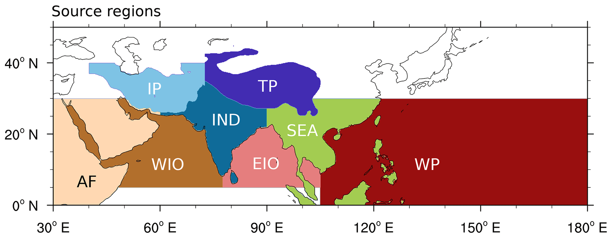
Figure 1 Source regions based on ERA-Interim orography and land–sea mask data at $\mathrm{0.125}{}^{\circ }\times \mathrm{0.125}{}^{\circ }$ grid spacing for the TRJ calculations. See text for details.

2.3.1 TRJ

For the trajectory model, the daily initialized (backward) trajectories are followed backwards in time based on the 6-hourly output of the data. Trajectory model data were calculated and analysed for 14 NH summer seasons (from 1 June to 31 August) out of the period 1979 to 2013, as the anticyclone showed a rather eastward (seven summer seasons) or westward location (seven summer seasons) during these years. Choosing these 14 years was motivated by the finding that anomalies of the vertical velocity in the AMA region are related to the position of the AMA (Nützel et al., 2016, their Fig. 14). For the selection, a modified version of the so-called South Asian High Index (SAHI; Wei et al., 2014), which measures the east–west displacement of the AMA, has been employed. The selected summer seasons are listed in Appendix A2, where also a description of the modified SAHI and of the selection process is presented.

2.3.2 EMAC–ATTILA

For the EMAC–ATTILA simulation, we use each of the 10-hourly output time steps of the model data and perform our analyses for 30 NH summer seasons (again, 1 June–31 August) from 1981 to 2010. Due to a processing error for the LG-K data, the year 2008 had to be removed. Further, all analyses were conducted based on the underlying EMAC model grid. In particular, for the analysis of EMAC–ATTILA data, the boundary layer source regions (see Fig. 1) were defined based on the underlying horizontal resolution of the base model.

2.4 Reanalysis data

ERA-Interim data (Dee et al., 2011; ECMWF, 2011) at $\mathrm{1.5}{}^{\circ }\times \mathrm{1.5}{}^{\circ }$ horizontal grid spacing are used to calculate the TRJ data. Additionally, ERA-Interim data (partly also at different resolutions) are employed for the interpretation of the TRJ data (e.g. to provide corresponding meteorological fields, land–sea masks, and orography) and in complementing analyses.

3 Trajectory model results

The focus of this study lies on the analysis of the trajectory model results (TRJ). Figure 2 shows the starting probabilities of trajectories located within the AMA, i.e. the fraction of days during JJA for which the starting positions of the trajectories are located within the AMA at 150 hPa at a certain grid point for the trajectory model calculations. The corresponding starting probabilities for years with a rather eastward or westward displacement of the AMA (see Appendix A2) are given as solid cyan and dashed magenta contours, respectively.

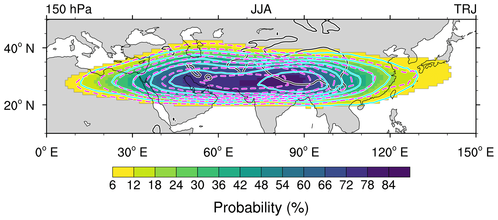
Figure 2 Probabilities (%) of starting locations for trajectories that start within the AMA at 150 hPa during JJA in the TRJ calculations. Trajectories were started daily at each $\mathrm{1}{}^{\circ }\times \mathrm{1}{}^{\circ }$ point within the region 10–50^∘ N ×0–150^∘ E and are said to be located within the AMA if the geopotential height anomaly from ERA-Interim (at 1.5^∘ grid spacing) was higher than 280 m (see text for further details). Again, black contours show the 2 km outline of ERA-Interim orography. Dashed magenta (solid cyan) contours (starting at 12 % in steps of 12 %) show the starting probabilities for the west (east) composites (see Sect. 2.3 for details).

3.1 Climatology and interannual variability

First, we investigate the climatological properties of the transport pathways and the PBL sources of air masses from the AMA in the TRJ data, with additional notes on the interannual variability (Sect. 3.1). For the analysis of the transport pathways, we will only consider trajectories that start within the AMA and reach the PBL within 90 d, whereas in the analyses of the PBL sources we also quantify the fraction of trajectories starting within the AMA that do not reach the PBL within 90 d (roughly 15 %; see Sect. 3.1.2). Besides the strong interannual variability, the AMA is also known for its intraseasonal/subseasonal variability (see, for example, Fig. 5 in Garny and Randel, 2013, showing both interannual and intraseasonal variability). Hence, the intraseasonal variability will be discussed thereafter (Sect. 3.2).

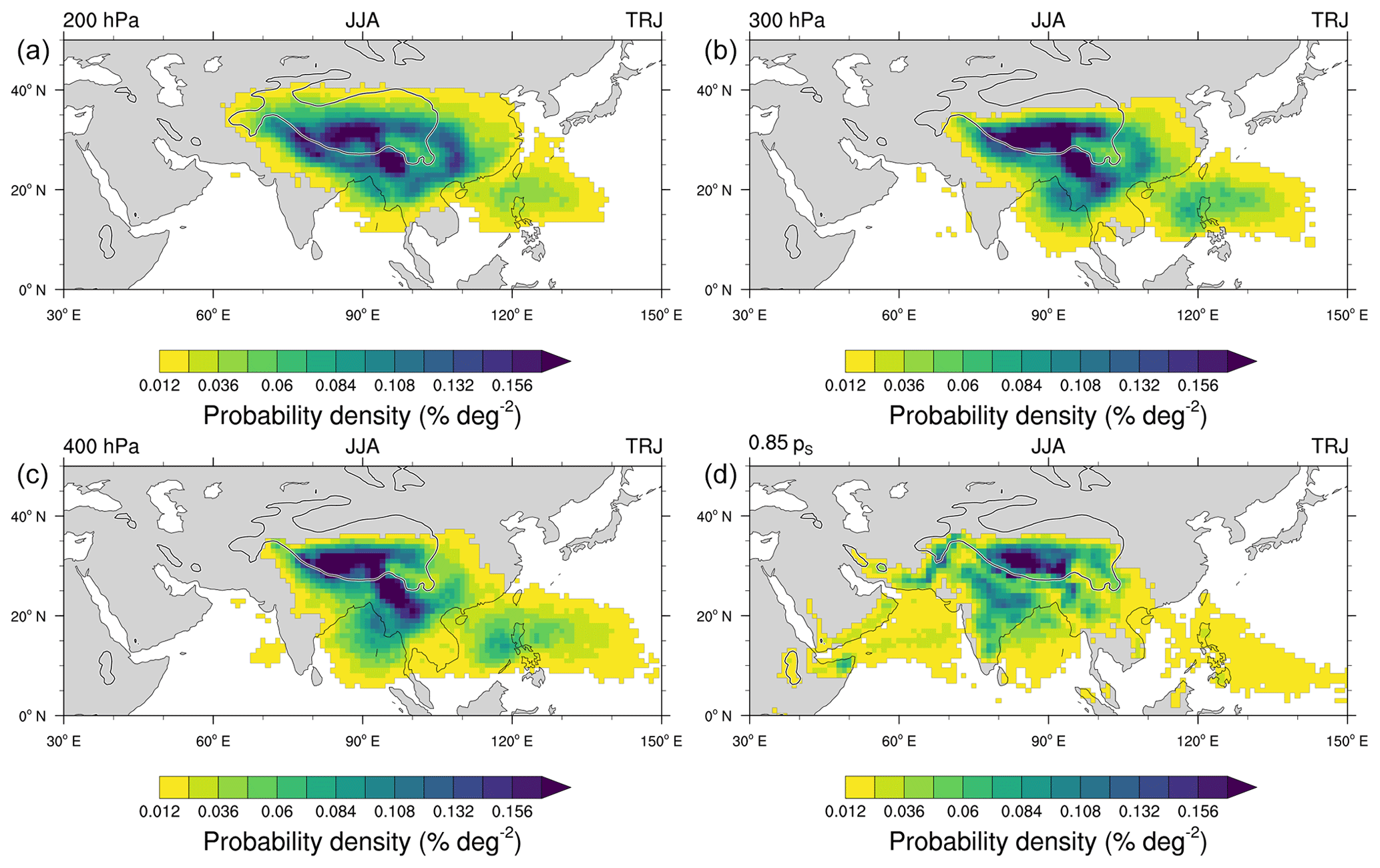
Figure 3 Probability density of upward crossings of trajectories (% deg⁻²) at (a) 200 hPa, (b) 300 hPa, (c) 400 hPa and (d) the PBL (defined as 0.85 times surface pressure) for trajectories that start within the AMA and cross the PBL (as defined before). As noted before, for the 14 years, the individual distributions have been calculated and averaged afterwards; i.e. each year contributes equally to the probability density (also for subsequent analyses). Here and in the following plots, if the last bin of the colour bar is denoted by a triangle, it contains all values up to the maximum of the field which is plotted.

3.1.1 Transport pathways

Figure 3 shows the probability density of final (i.e. first going back in time from the 150 hPa level) upward crossing locations of trajectories for specific height levels, i.e. 200, 300 and 400 hPa and the boundary layer (defined as 0.85 times surface pressure) in the TRJ calculations. This analysis is analogous to the analysis shown, for example, in Fig. 4 of Bergman et al. (2013). In all panels, only trajectories that reach the PBL within 90 d of their release are accounted for. Our results show that during JJA on a climatological basis, AMA air mass sources come from a broad region in the PBL in Asia (Fig. 3d). With increasing height, the upward transport of air masses focuses on (the region below) the south-eastern part of the AMA. Thus, our multiannual trajectory analyses support the findings for August 2011 presented by Bergman et al. (2013) regarding the final crossing points of the PBL of trajectories that ascend to the AMA.

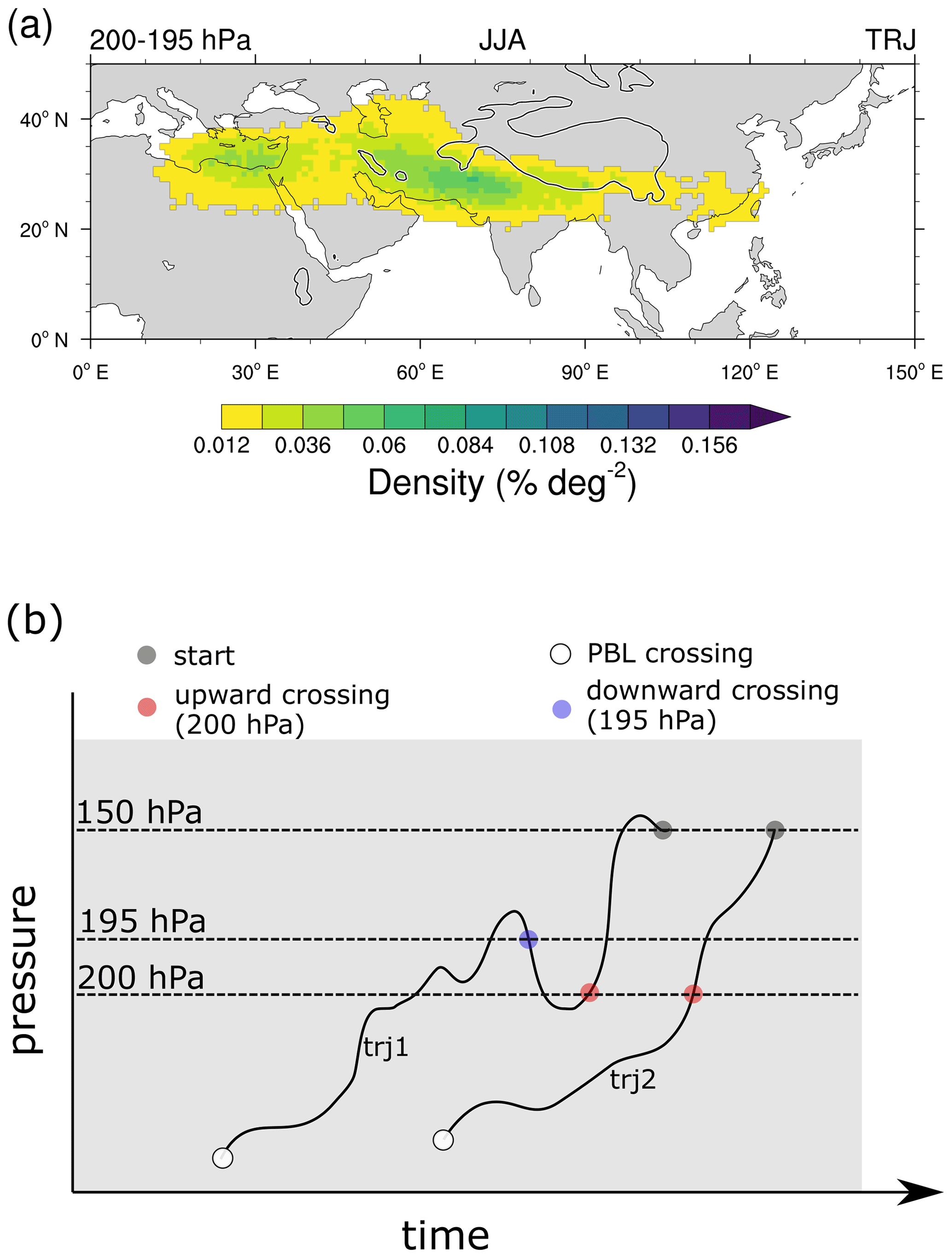
Figure 4 (a) Density of downward crossings of trajectories (% deg⁻²) at 195 hPa for trajectories that start within the AMA and cross the PBL (as defined before) and fall below 200 hPa before they reach the final destination at 150 hPa. Roughly 60 % of the PBL crossing trajectories experience this downward crossing, and the coloured area corresponds to roughly 32 % of the PBL crossing trajectories. (b) Schematic of trajectory crossings described in panel (a) and in Fig. 3. See text for details.

However, we point out that by construction, this analysis only shows the regions where trajectories that reach the 150 hPa level in the AMA experience their final upward transport through the respective level. Hence, it can not be inferred from this analysis that the trajectories are located strictly within these upward transport regions throughout their pathway from the PBL to the 150 hPa level within the AMA. And indeed, this is not the case as can be seen from Fig. 4a, which shows the density distribution of trajectories that have fallen below 200 hPa and have risen again above 195 hPa (backward in time). This analysis points out the locations of downward transport which are located on the western side of the AMA. Approximately half of all PBL crossing trajectories experience this downward motion at the depicted level and hence must traverse this region on their pathway to the 150 hPa level within the AMA.

To simplify the interpretation, a clarifying schematic for two hypothetical PBL-crossing trajectories (trj1 and trj2) is shown in Fig. 4b: the positions of trj1 and trj2 at the red dots would be noted in Fig. 3 – showing regions of upward transport, i.e. the final crossing points of a certain level of the trajectories. In contrast, the position of trj1 at the blue dot would be noted in Fig. 4b – highlighting regions of downward transport.

Figure 5 Longitude versus log-pressure height cross sections of density distributions (% deg⁻¹ km⁻¹, i.e. percent per degree per kilometre) of trajectory positions for PBL crossing trajectories (a) 1 d, (b) 2.5 d, (c) 5 d and (d) 15 d prior to their arrival at 150 hPa within the AMA. The three-dimensional probabilities were integrated over 0–50^∘ N. Please note the different colour bars. Once trajectories reach the PBL, their pathways are not followed back any further. Instead, they are also noted at their first PBL-crossing points for analyses going back further in time. For example, if a trajectory already reaches the PBL after 3 d, it will also be counted at this PBL-crossing position for the analysis 5 and 15 d back in time. Please note – also for upcoming figures – that the maximum in the distribution at 4–6 km, for example, present in panel (d), is related to the TP. Cyan lines indicate potential temperature levels at 30^∘ N starting at 340 to 380 K in steps of 10 and 20 K afterwards (380 to 480 K). Black contours indicate meridional winds at 30^∘ N in steps of 3 m s⁻¹. Negative, i.e. southward, winds are dashed, and the zero wind line is given in orange. Meteorological data based on ERA-Interim are flagged out below the grey line, which indicates the ERA-Interim minimum surface pressure in the region 0–50^∘ N of the time average JJA for the trajectory years.

To get a better picture of the pathways of the trajectories, we show the distributions of PBL crossing trajectories as a longitude vs. log-pressure height cross section in Fig. 5. The log-pressure height was calculated with a scale height of 7 km (see, for example, Abalos et al., 2017) and with the reference pressure of 1013.25 hPa as in the base model of the EMAC–ATTILA simulations (see Roeckner et al., 2003, for details on ECHAM5). The individual panels show the temporal evolution of the trajectories that start within the AMA, 1, 2.5, 5 and 15 d prior to their release (panels a–d, respectively). For orientation purposes, meteorological data from ERA-Interim are overlaid (see figure caption for details).

Obviously, as noted by Bergman et al. (2013), the main upward transport occurs on the south-eastern side below the anticyclone (centred around ∼90^∘ E); however, as already indicated above, the trajectories start to fill the AMA well below the initial release height (150 hPa), and downward transport occurs on the western side of the AMA (Fig. 4a). It is worth noting that 15 d prior to release, a considerable fraction of trajectories has reached the PBL above the TP (maximum in the density around 5 km and 70–100^∘ E in Fig. 5d).

Figure 6 Latitude versus log-pressure height cross sections of density distributions (% deg⁻¹ km⁻¹) of trajectory positions for PBL crossing trajectories 5 and 15 d prior to their arrival at 150 hPa within the AMA. The three-dimensional probabilities were integrated over 60–140^∘ E. Once trajectories reach the PBL they are not tracked further and will also be noted at the crossing point further back in time (as in Fig. 5). Cyan lines indicate potential temperature levels averaged over 0–120^∘ E starting at 340 to 380 K in steps of 10 and 20 K afterwards (380 to 480 K). Black contours indicate zonal winds averaged over 0–120^∘ E in steps of 5 m s⁻¹. Negative, i.e. westward, winds are dashed, and the zero wind line is given in orange. Meteorological data based on ERA-Interim are flagged out below the grey line, which indicates the ERA-Interim minimum surface pressure in the region 0–120^∘ E of the time average JJA for the trajectory years.

The complementing latitude versus log-pressure height cross section of the climatological trajectory positions for JJA is shown in Fig. 6. Here, the trajectory positions (Fig. 6a) 5 and (Fig. 6b) 15 d prior to their arrival at 150 hPa are depicted. Again, meteorological data from ERA-Interim is overlaid to facilitate the interpretation. The trajectory distribution around the AMA height levels is tilted from North to South, in agreement with a tilt of the isentropic levels (see cyan lines in Fig. 6). We note that the distribution shows high values above or around the slopes of the Himalayan mountains (roughly at 30^∘ N) and that over time more and more trajectories reach their PBL source region over the TP (max. around 5 km and 30–35^∘ N) and to its south.

From the presented analyses, the emerging picture of PBL-to-AMA transport, which shows focused regions of upward transport below the south-eastern side of the AMA and recirculation with upward (downward) transport on the eastern (western) side of the AMA, is in agreement with upward circling, which follows the first updraft as described by Vogel et al. (2019) and Legras and Bucci (2020). The diagnosed recirculation within the AMA, well below the release height of the trajectories (see Figs. 4a and 5), refines the original conduit schematic as depicted and discussed by Bergman et al. (2013). The transport pathways further fit with the distribution of mean vertical velocities in the UTLS in the monsoon region (e.g. Nützel et al., 2016, their Fig. 10) as well as tracer transport and distribution in a CCM as discussed by Pan et al. (2016; see also their discussion on the large-scale circulation in the AMA region). Additionally, CO distributions from chemistry transport model data presented by Barret et al. (2016) support this view on PBL-to-AMA transport, while in their climatological analysis of IASI satellite data, the structure was not as conclusive. Using data from the same satellite instrument, but performing transient analyses, Luo et al. (2018) came to the conclusion that this transport behaviour is also present in the satellite data. Similarly, Vogel et al. (2019) noted that the CO transport described by Pan et al. (2016) is in agreement with their results from a trajectory model and MIPAS satellite data. We stress here that the trace-gas-based results (e.g. in modelling or satellite data) also strongly depend on the strength and location of emissions, whereas the idealized trajectory studies simply track air mass transport.

We will now address the sensitivity of the presented results to east–west shifts of the AMA on interannual timescales. Therefore, Fig. 7 shows the differences in the upward transport regions for west minus east years. Differences are clear in the upper level (200 hPa) and fit to the corresponding differences of the vertical wind fields at 150 hPa (not shown). The differences are less pronounced at the top of the PBL (defined as 0.85 times surface pressure).

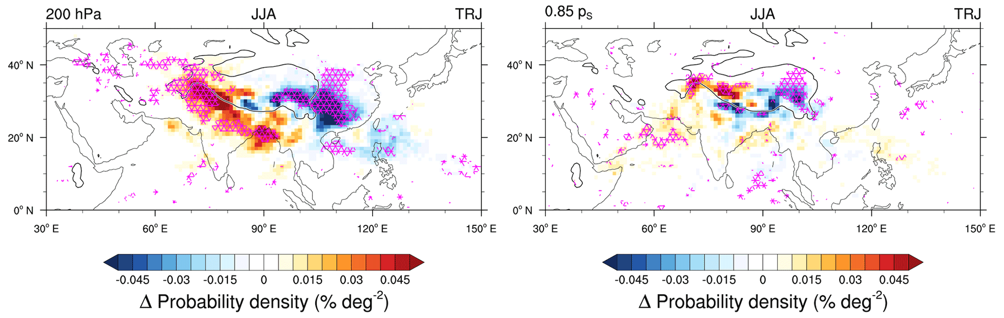
Figure 7 Difference (west minus east years) of probability densities of trajectory upward crossings (% deg⁻²) at 200 hPa and the PBL (defined as 0.85 times surface pressure) for trajectories that start within the AMA and cross the PBL (as defined before). The underlying fields have been horizontally smoothed, and the significance level of 0.1 is noted via magenta hatching.

To capture the differences of the trajectory pathways between years with a rather western and rather eastern position of the AMA, Fig. 8 shows the corresponding composite differences (west minus east) of the analyses in Fig. 5. Whereas differences are pronounced and significant shortly after the release of the trajectories in the UT, they get less pronounced and clearly less significant at lower levels. Overall, there are no qualitative differences in the transport pathways between years with a rather eastward location of the AMA and years with a rather westward location of the AMA.

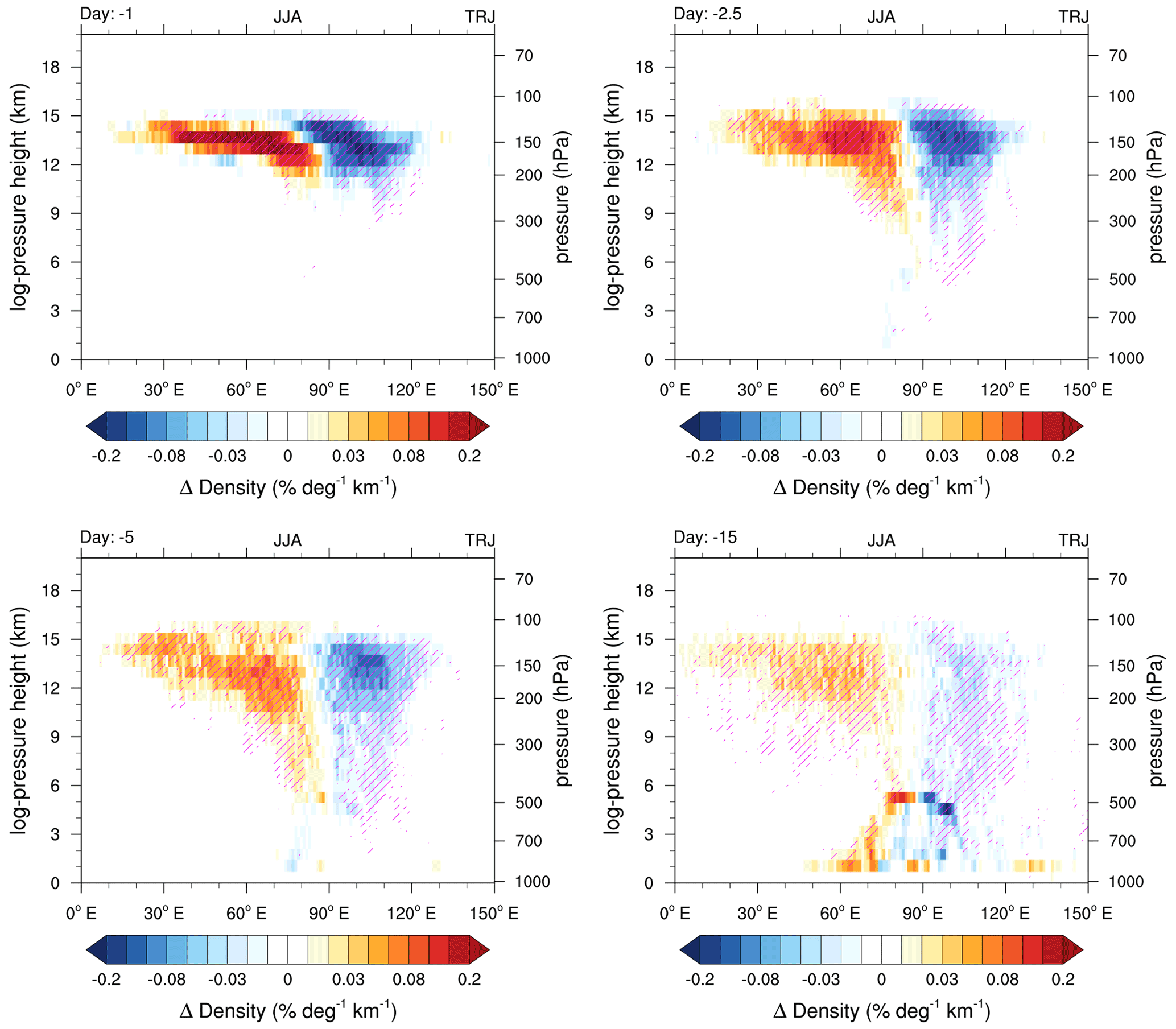
Figure 8 Longitude versus log-pressure height cross sections of the difference (west minus east years) of the density distributions (% deg⁻¹ km⁻¹) of trajectory positions for PBL crossing trajectories 1, 2.5, 5 and 15 d prior to their arrival at 150 hPa within the AMA. The three-dimensional probabilities were integrated over 0–50^∘ N. Once trajectories reach the PBL, they are not tracked further and will also be noted at the crossing point further back in time (as in Fig. 5). Magenta hatching indicates the 0.1 significance level.

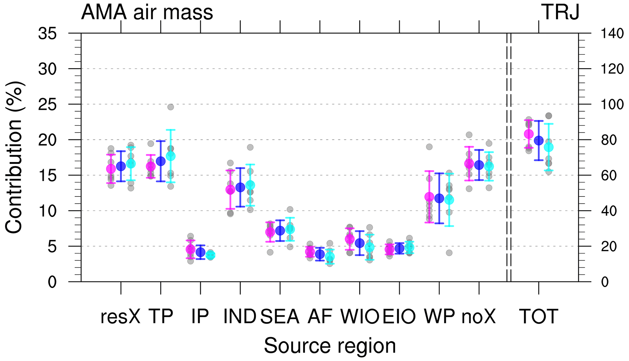
Figure 9 Contributions from different source regions to AMA air masses at 150 hPa during JJA. The categories resX and noX correspond to the trajectories that reached the PBL outside the defined source regions (see Fig. 1) or did not reach the PBL within 90 d prior to their start, respectively. TOT corresponds to the total numbers of trajectories released within the AMA and is given in units of 10³ trajectories. The mean values are given by blue dots with blue whiskers for the interannual standard deviation. The mean values and interannual standard deviation split according to the east (west) location of the AMA are given as cyan (magenta) dots and whiskers, and the individual years are shown as grey dots.

3.1.2 Boundary layer source regions

In the following, we want to further analyse from which PBL source regions (see Fig. 1) air masses within the AMA originate. For these analyses, the fraction of the trajectories which start within the AMA but do not reach the PBL within 90 d is also accounted for. The mean contributions of individual source regions (blue dots) in the TRJ simulation and their interannual variations (translucent grey dots and blue whiskers) are shown in Fig. 9. The largest contributions from the named source regions are found from the TP region (around 17 %), the IND region (around 13 %) and the WP region (around 12 %). However, we note that the densities of PBL crossings are larger for the TP and IND region than for the WP region (see Fig. 3). There is also a considerable fraction of trajectories of around 16 % that encounter the PBL outside the named source regions (resX) or do not encounter the PBL within 90 d prior to release (noX).

There is strong interannual variability regarding the sources of the AMA, as indicated by relatively large whiskers and a considerable spread of the contributions in individual monsoon seasons. Nevertheless, the aforementioned regions, namely TP, IND and WP, are more important for the AMA composition in the TRJ simulation in almost all years than the other source regions. The intraseasonal variability of these source regions will be discussed along with the variability of the transport pathways in the next section (Sect. 3.2).

Concerning the interannual east–west shifts of the AMA, there are no substantial differences of the PBL source regions and of the fraction of non-crossing trajectories (cyan and magenta dots in Fig. 9). This is in agreement with the previous finding that the main transport pathways did not change qualitatively (see Fig. 8) and that the boundary layer source changes are relatively small or partly compensated for within the different source regions as for instance for the TP region (see Fig. 7). Slightly more trajectories are located within the AMA for years in which the AMA is displaced to the west (in agreement with the higher maximum in the contour lines for westward location of the AMA in Fig. 2). However, the large interannual variability (whiskers in Fig. 9) renders this and other small differences between the two composites insignificant.

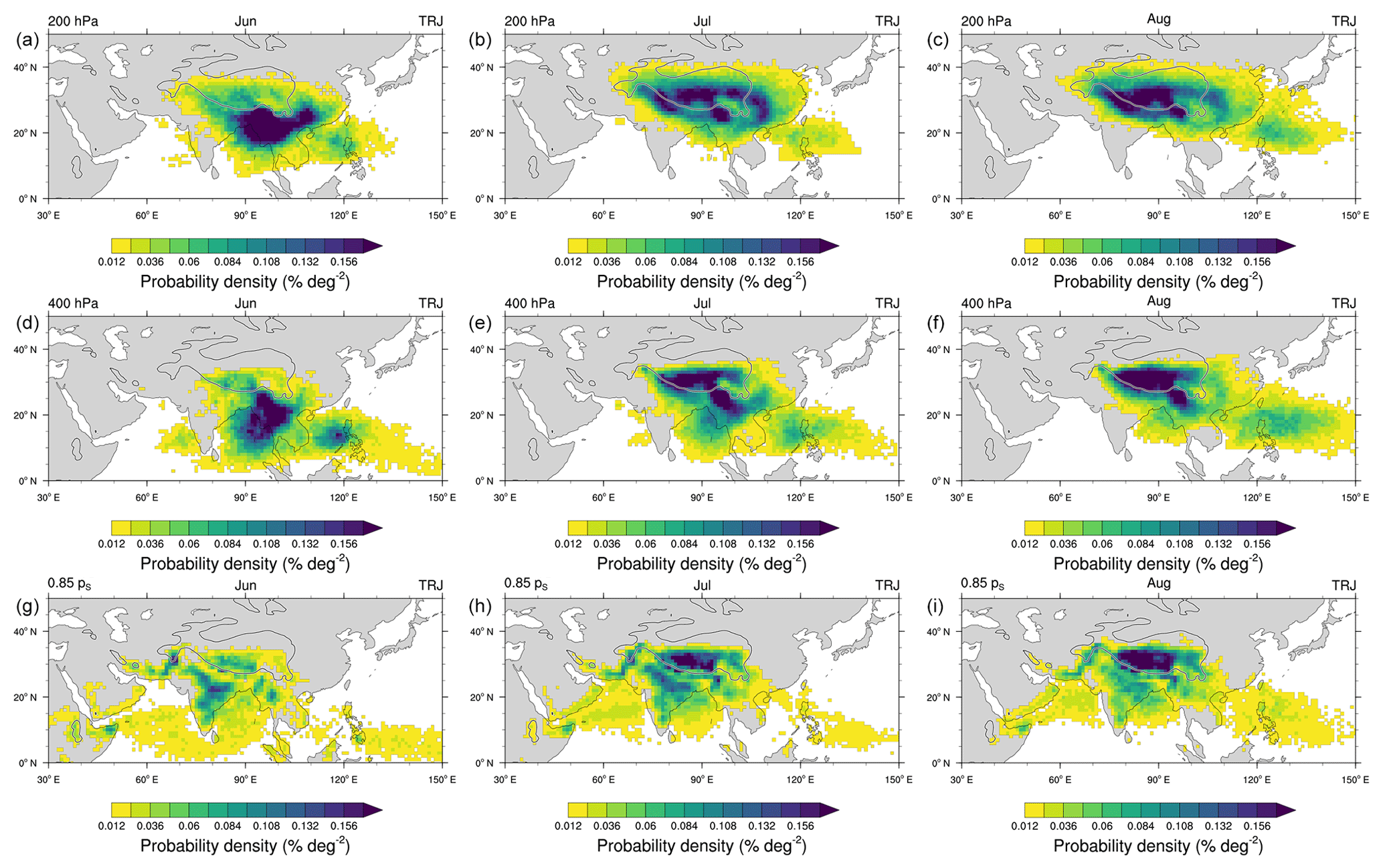
Figure 10 Probability density (% deg⁻²) of trajectory (upward) crossings at (a, b, c) 200 hPa, (d, e, f) 400 hPa and (g, h, i) the PBL as in Fig. 3 but split according to (a, d, g) June, (b, e, h) July and (c, f, i) August.

3.2 Intraseasonal variability

3.2.1 Transport pathways

To further analyse the subseasonal variability of the PBL source regions and the transport pathways of the PBL-crossing AMA trajectories, Fig. 10 (analogous to Fig. 3) shows maps of final boundary layer and pressure level crossings split according to June, July and August, respectively. As can be seen from these plots, the PBL crossings shift over continental Asia over the course of the monsoon season from June to August. Furthermore, the regions of upward transport, which are mainly centred over the eastern Indian Ocean (Bay of Bengal), and adjacent continental regions at 200 and 400 hPa in June shift northwards towards the TP in July and August.

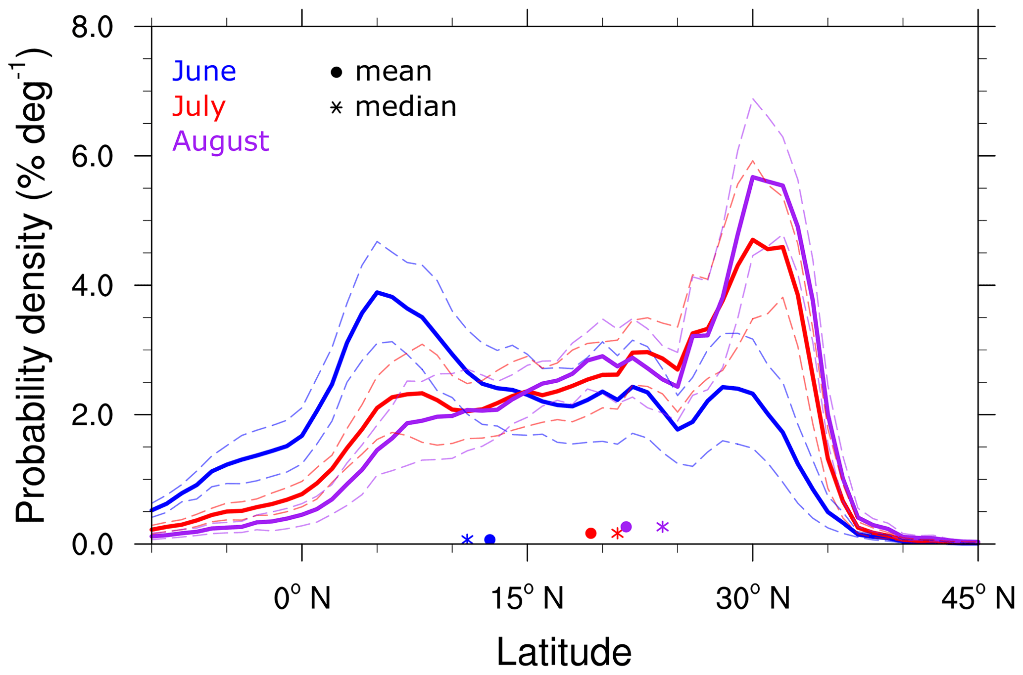
Figure 11 Probability density (% deg⁻¹) with respect to latitude of trajectory intersections with the PBL split according to June (blue), July (red) and August (purple). Mean (dots) and median (crosses) are given as well. Dashed lines mark the interannual standard deviation.

A more quantitative view of this northward shift is presented in Fig. 11, which shows the distributions of the latitudinal position of PBL crossings for June (blue), July (red) and August (purple) of trajectories starting in the AMA. In particular, the modal value in June at 5^∘ N is clearly reduced in July (and August), and the contributions around 30^∘ N roughly double from June to July. The interannual variability depicted as dashed lines in Fig. 11 allows the conclusion to be drawn that this is a typical behaviour throughout the monsoon season.

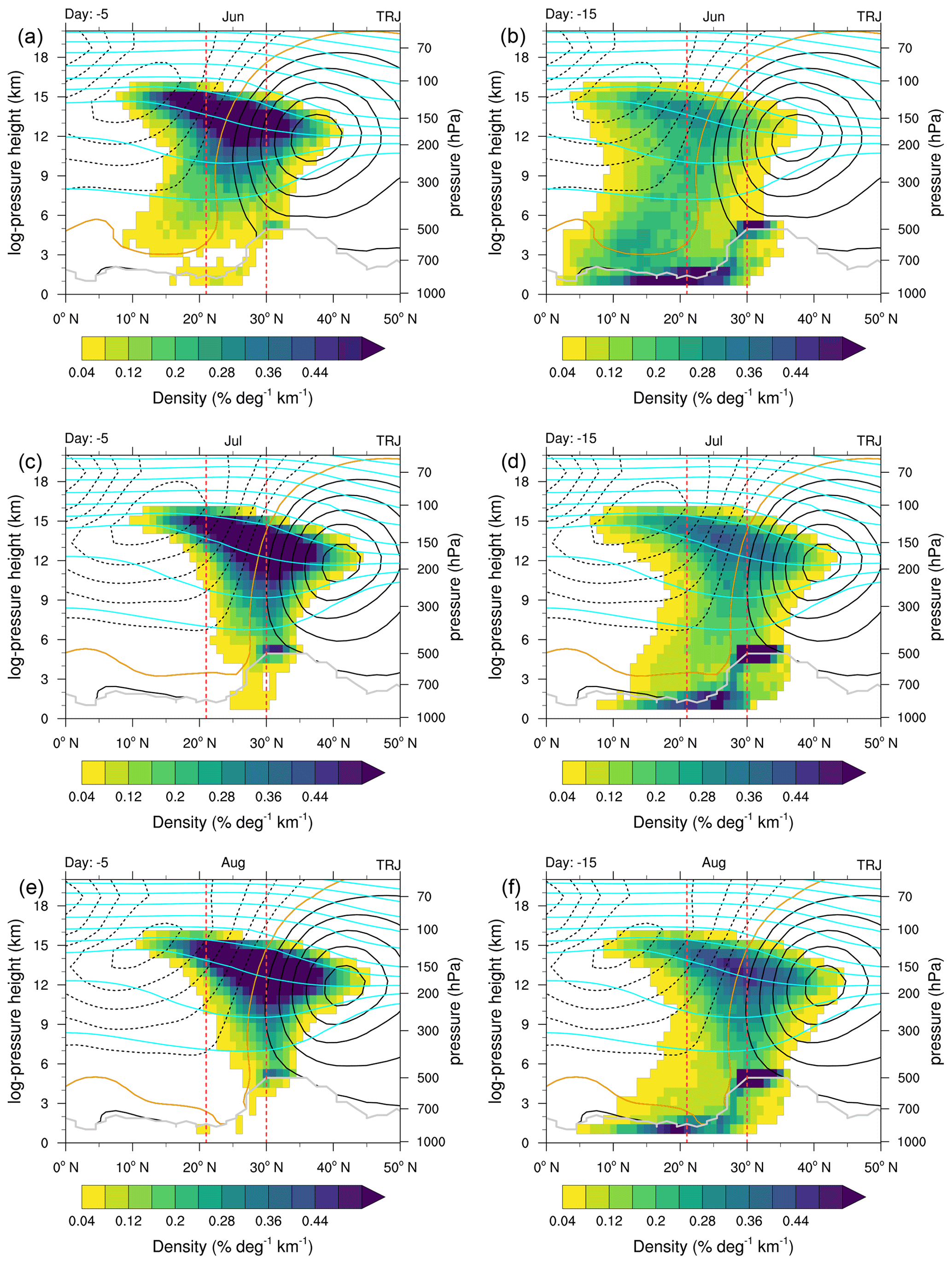
Figure 12 As in Fig. 6 for (a, c, e) 5 and (b, d, f) 15 d prior to their final position at 150 hPa, split according to (a, b) June, (c, d) July and (e, f) August. Again the three-dimensional probabilities were integrated over 60–140^∘ E. For orientation purposes, dashed vertical red lines at 21 and 30^∘ N roughly indicate the maxima in the distributions between 6 and 12 km for June and August for the trajectories 15 d prior to their arrival at 150 hPa, respectively. Meteorological data from ERA-Interim are presented as in Fig. 6 but separated for June, July and August, respectively. At the bottom, data were flagged with the same criterion as in Fig. 6.

For a complementing view of the transport pathways during June to August, Fig. 12 shows the distributions of the trajectories in a latitude versus log-pressure height cross section 5 and 15 d before the trajectories encounter their starting position at 150 hPa. It is shown that the trajectory locations shift from south to north during the evolution of the ASM from June to August. In August, the AMA is located above the TP, and air masses from the TP can directly feed into the core of the AMA. We emphasize the clear shift of the maximum density at about 6 to 10 km from approximately 20^∘ N in June to 30^∘ N in August.

Figure 13 (a) Temporal evolution of source region contribution to the AMA air masses at 150 hPa in the TRJ calculation. To fit the scale, the resX category was scaled by 0.5. All contributions have been smoothed using 5 d running means (weights of $\left[\frac{\mathrm{1}}{\mathrm{9}},\frac{\mathrm{2}}{\mathrm{9}},\frac{\mathrm{3}}{\mathrm{9}},\frac{\mathrm{2}}{\mathrm{9}},\frac{\mathrm{1}}{\mathrm{9}}\right]$). (b) Contributions of PBL sources to the AMA at 150 hPa for the TRJ calculation over 14 years split according to June (blue), July (red) and August (purple). The interannual standard deviation is given as whiskers, and the individual years are included as grey dots. For TOT the total number of trajectories is given in units of 10³ trajectories.

3.2.2 Boundary layer sources

Figure 13a shows the temporal evolution of the source region contributions to the AMA air masses in the TRJ simulation. To provide the full budget, the fraction of the non-crossing trajectories (noX) is also shown. The most prominent change is the increase of the TP contribution from below 4 % in early June to more than 24 % for most of August. Also, it is obvious that the fraction of non-crossing (noX) trajectories clearly decreases over time. This implies that over the monsoon season, the fraction of air masses within the AMA that have recently (within the last 90 d) come from the PBL increases. Further, over the course of the monsoon season, the contributions of trajectories that cross the PBL outside the monsoon region (resX) declines noticeably. This indicates that the PBL sources focus more toward the Asian monsoon region and is in accordance with the impression from Fig. 10. The WP region shows a minimum contribution at the beginning of July (below 10 %), whereas the contributions in early June (around 16 %) and the end of August (around 20 %) are clearly higher. For the IND region, the evolution is reversed, with a peak contribution in July (∼16 %) and lower contributions in early June and end of August (about 8 % and 12 %, respectively). Apart from a small dip in early June, the contribution of the SEA region increases steadily from around 5 % in mid-June to approximately 9 % end of August. For the AF region, this behaviour seems to be reversed (from around 5 % to 3 %). All other source regions (WIO, EIO and IP) show some variation in June but have relatively stable contributions (between about 4 %–6 %) during July and August.

Figure 13b shows the source region contributions split according to June, July and August. The increase in the contribution of the TP from June to August is pronounced and present in every single year. Thus it is a robust feature of the intraseasonal variability of AMA air mass contributions. Further, except for 1 year, the TP is the most important source region for air masses within the AMA in August in our analysis. Also, as the resX contribution significantly declines from June to July/August, it is shown that the PBL source regions focus more on the ASM region. More trajectories are located within the AMA in July than in June and August, which is in agreement with the seasonal cycle of the AMA (e.g. Garny and Randel, 2013; Nützel et al., 2016, Figs. 5 and 12, respectively), as already described by Mason and Anderson (1963). For the other source regions, the intraseasonal variations are overruled by the strong interannual variability, and more years would be needed to carve out robust differences.

4 EMAC–ATTILA results: a complementary view

To corroborate our results and to point out sensitivities and uncertainties, we also show the results of free-running Lagrangian CCM simulations. As already noted in Sect. 1, the Lagrangian data from these simulations can provide a complementary view because the modelling approach differs largely from the reanalysis-driven trajectory data presented in Sect. 3. The EMAC–ATTILA data contain the effect of parametrized convection and stem from two free-running simulations, in which the vertical velocity is described either by a kinematic (LG-K) or a diabatic (LG-D) scheme (see Sect. 2).

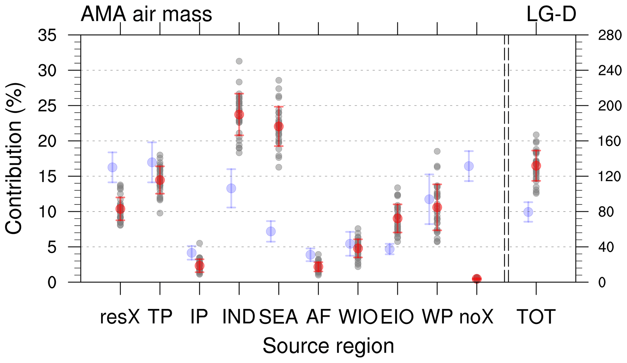
Figure 14 Contributions of PBL sources to the AMA around 150 hPa for 1981–2010 from the free-running LG-D simulation. Mean values are given as red dots, red whiskers denote the interannual standard deviation and individual years are indicated as grey dots. For TOT the right axis denotes the total number of trajectories in units of 10³ trajectories. For comparison, faint blue dots and whiskers denote the values from the TRJ data.

First, we want to focus on features where the LG-D simulation support the results of the TRJ calculations. Secondly, we show which results differ and where (a parametrization of) Lagrangian convection might be of importance. Finally, we also address the impact of the vertical velocity scheme by comparing the model results of the LG-D and LG-K.

We have found that the pathways of the LG-D data (see Appendix Fig. B2) look similar to the pathways shown in Fig. 5. Moreover, the LG-D data also show strong interannual variability in the source region contributions (see Fig. 14).

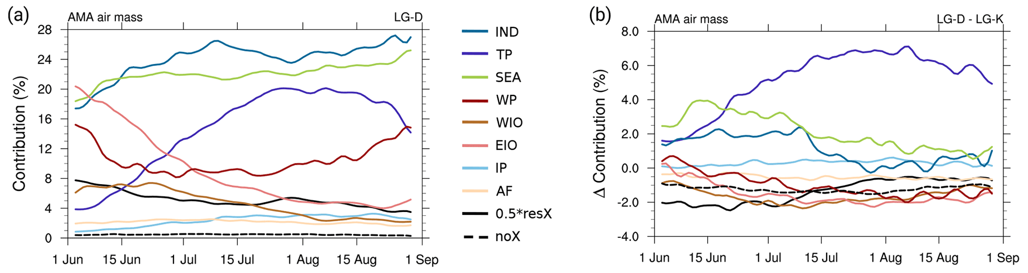
Figure 15 (a) PBL source contribution evolution in the LG-D data. resX data have been scaled by 0.5. All contributions have been temporally smoothed using 5 d running means (weights of $\left[\frac{\mathrm{1}}{\mathrm{9}},\frac{\mathrm{2}}{\mathrm{9}},\frac{\mathrm{3}}{\mathrm{9}},\frac{\mathrm{2}}{\mathrm{9}},\frac{\mathrm{1}}{\mathrm{9}}\right]$), while daily data were produced from summing up the 10-hourly data for each day. Panel (b) is as in (a) but for the difference of the source contributions for LG-D minus LG-K. As in the LG-K data the year 2008 is missing (see Sect. 2.3), it was also removed in the LG-D data for this analysis. Colour coding as in (a).

Further commonalities in the TRJ and LG-D model data results can be seen when it comes to the evolution of PBL contributions to the AMA air masses. Both model data show an increase of the TP contribution from June to August (Figs. 13 and 15a). Also, the qualitative evolution of the contribution of the WP and SEA regions – minimum contribution during July for WP and slight increase over the monsoon period for SEA – is similar in the two model data sets.

However, we have to note that quantitatively, the contributions differ between the two model data sets (see also Fig. 14). As an example, the contribution of the TP in August is not as dominant in LG-D as in TRJ. Further, around 11 % of the trajectories come from a region outside the defined sources in the LG-D, which is similar to roughly 16 % in the TRJ data. However, in the TRJ data, this contribution drops considerably from June to August, whereas in the LG-D data, the decline is more moderate.

The differences between the TRJ and EMAC–ATTILA data are likely to also be related to the faster vertical transport in the LG-D data due to the effect of parametrized convection. As an example, the air masses that do not reach the PBL within 90 d account for more than 15 % in the TRJ calculation during JJA, whereas in LG-D this value is below 1 %. The differences in this fraction might also be related to the quantitative differences in the contributions of IND and SEA in the TRJ and LG-D data, namely clearly higher contributions in the LG-D data than in the TRJ calculations. An intermediate region is the EIO showing slightly higher contributions in LG-D data, which might hint towards the importance of convective transport from this region, which is located beneath the south-eastern part of the AMA. As the contributions of IP, AF and WIO are relatively small in all model data sets, this indicates that transport from these regions to the AMA might not be overly important.

We stress that the above results also hold qualitatively for the LG-K data. Figure 15b shows the differences in the contribution of source regions to the AMA air masses for LG-D minus LG-K data. Major differences are that the contribution of the TP is not as large as in the LG-D data and that the increase over the monsoon period is less pronounced (absolute values for LG-K are shown in Fig. B4 in the Appendix B). Throughout the monsoon season, the LG-D data show overall higher contributions for TP, IND and SEA compared to the LG-K data. Almost no differences are found for the contribution of the IP, whereas lower contributions are found for the other source regions.

As we have found a strong increase of the TP contribution to the AMA air masses over the monsoon season in the TRJ and LG-D (less so in LG-K) data, for the LG-D data we further analysed the change of transport properties from the TP to the UT for June and August. Therefore, Fig. 16 shows the differences (August minus June) in the longitudinal distributions of trajectories that stem from the TP for multiple pressure levels (300–150 hPa in steps of 50 hPa). In August compared to June, the trajectories are more likely located in the ASM region (60–100^∘ E), whereas in June compared to August, the probability is larger east of the ASM region (and in particular the North American monsoon region sticks out). Further, the fraction of trajectories from the TP at the different levels (June divided by August) also decreases with height (from about 90 % at 300 hPa to about 70 % at 150 hPa), which indicates that transport from the TP to the UT is stronger in August than in June. These results are consistent with stronger advection to the east of air masses from the TP in June compared to August due to the location of the subtropical jet.

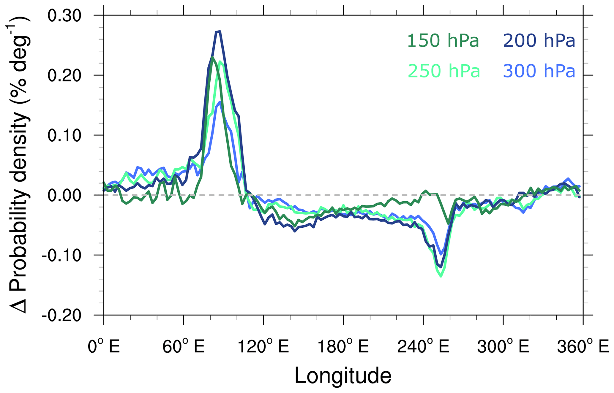
Figure 16 Difference (August minus June) of longitudinal probability densities of parcels that originate from the TP at various pressure levels in the UT based on 1981–2010 for the LG-D data.

We want to point out that the results of EMAC–ATTILA (in particular as they come from a free-running simulation) should not be seen as validation data but rather as a help to assess which key transport characteristics are present in these data as well. This might help to discern which processes/source regions are not heavily dependent on the inclusion of convection through a parametrization and the detailed meteorology (free-running CCM versus TRJ calculations driven by reanalysis data). As an example, the contributions from the source regions TP, WP and SEA show similar developments over the course of the monsoon period, although the quantitative contributions partly differ. Further, the fact that the LG-D and LG-K simulations show discrepancies in parts, for example, with respect to the mean contributions of the TP of slightly above 14 % and 9 % (see Figs. 14 and B3), despite being driven by identical meteorological states of the host model, highlights the influence of the vertical velocity scheme to parts of the analyses. Here, we note that this might be partly already caused by the different distributions of the air parcels in LG-D vs. LG-K data: as the air parcels persist throughout the simulation and are transported with different vertical velocities, the distribution of air parcels within the AMA differs between the two model data sets (see Appendix Fig. B1), even though the same dynamical constraints are used to define the AMA. We are currently planning future work to further carve out the transport properties in the ASM region based on additional Lagrangian CCM simulations.

5 Discussion

5.1 Relation to previous modelling results and observational data

In Sect. 3 we have presented results regarding the transport from the PBL to the AMA based on our trajectory calculation (TRJ). We have found that the boundary layer source distribution (Figs. 3 and 10) focuses over the ASM region (in particular over the Indian subcontinent and the TP). Further, these distributions support previous results regarding the PBL sources of the air masses of the AMA and its surroundings, for example, by Bergman et al. (2013) and Fan et al. (2017). Similarly, the boundary layer crossing distributions are in agreement with convective source maps of the AMA as presented by Legras and Bucci (2020).

Moreover, we found similar regions of upward transport as Bergman et al. (2013), which are located on the south-eastern side of the AMA. However, we also complemented the view about the transport pathways, i.e. the conduit proposed by Bergman et al. (2013), by showing that air masses spread earlier in the AMA volume – in agreement with the transport pathways described by Vogel et al. (2019) and Legras and Bucci (2020). Combining our results with previous studies shows that the transport pathways as diagnosed by (i) a trajectory model including mixing effects (Vogel et al., 2019), (ii) a trajectory model including the effect of observed convection (Legras and Bucci, 2020), (iii) more puristic trajectory models (Bergman et al., 2013, and this study) and (iv) forward trajectories (analysed backwards in time) from a Lagrangian model with parametrized convection driven by a free-running CCM (this study) are in agreement. Further, the transport pathway is also supported by (v) analyses of CO transport within a CCM and a chemistry transport model as shown by Pan et al. (2016) and Barret et al. (2016) and (vi) analyses of satellite data (Luo et al., 2018; Vogel et al., 2019). In particular, our results also show that, although there is interannual and strong intraseasonal variability, the main transport characteristics are robust.

As noted by Legras and Bucci (2020; see end of their Sect. 3.1), there is a discrepancy between precipitation maps and source maps of the AMA air masses. Similarly, Bergman et al. (2013) have discussed the relation of the position of strong vertical winds and their so-called conduit, i.e. the region of upward transport for trajectories that reach the AMA (see their Fig. 7 and Sect. 5). We note that precipitation maps from observations (e.g. Xie et al., 2006, their Fig. 1) also do not directly correspond to high cloud distributions in the Asian monsoon region, as shown by Devasthale and Fueglistaler (2010). Further, it is noted by Shige and Kummerow (2016) that orographic precipitation over west India is often related to low clouds. Based on these previous studies and our analyses, our understanding is as follows: low- to mid-level convection might be important for the precipitation patterns, but air parcels that are transported upwards in this convection need to find a region of onward transport to the AMA. Seemingly, for some of the regions with heavy precipitation, this rarely happens.

Regarding the source regions, our results are in agreement with some of the results found in previous studies, while keeping in mind that there are (sometimes subtle) differences in the study design: as an example, Bergman et al. (2013) found that roughly 27 % of the all trajectories located in the AMA at 200 hPa come from the TP¹, which is similar to the mean contribution of the TP in August in the TRJ data of this study (slightly more than 24 %; about 25 % for August 2011). The combined area and contribution (again roughly 25 % in August; about 26 % in August 2011 in the TRJ data) of the regions IND, IP and SEA is comparable to the area and contributions (roughly 32 %)² of the Asian land masses excluding the TP, as analysed by Bergman et al. (2013). Further, Vogel et al. (2015) showed contributions of PBL sources to the AMA at 380 K. Although the TP was not explicitly resolved in their study, the contributions of the source regions used in their study, which cover the TP (red and green lines in their Fig. 8), show a strong increase from June to late July. This increase is in agreement with the increase of the TP contribution found in our study. The dependence of the TP contribution to AMA air masses on the position of the AMA is in analogy to the relation of typhoon–AMA transport discussed by Li et al. (2017); i.e. for the TP or typhoons, entrainment of air masses uplifted from these sources into the core of the AMA depends on the co-location of the AMA and the TP or typhoon, respectively.

Further, the northward shift of the PBL source regions and the transport pathways is consistent with the northward shift of the region of low outgoing longwave radiation and the AMA (Nützel et al., 2016, their Fig. 12; see also the related discussion) and the monsoon (precipitation) itself (e.g. Wang and LinHo, 2002; Yihui and Chan, 2005). This northward propagation can also be seen in deep convective activity as monitored by satellite measurements, where deep convection (up to 150 hPa) over the TP is rare in June and becomes more prominent in July and August (Devasthale and Fueglistaler, 2010).

Goswami et al. (1999) defined an index for the interannual Indian monsoon variability, the so-called monsoon Hadley index (MHI), as meridional wind shear between the UT (200 hPa) and the 850 hPa level over a reference region and motivate their definition by the relation to heating released due to precipitation in the respective region. Here we calculate the MHI from ERA-Interim data based on JJA data. We find that the detrended MHI and (modified) SAHI are strongly anti-correlated (−0.68) over the period 1979–2013, and in particular the anti-correlation for the years where the SAHI is anomalous (i.e. the 14 monsoon seasons for which the backward trajectories have been calculated) is even higher (−0.83). This hints that by analysing years with rather strong displacements of the AMA to the east or the west, we have implicitly analysed the impact of the detrended MHI on the transport properties from the PBL to the AMA.

5.2 Uncertainties in the presented results

The representation of convective transport in the trajectory analyses forms the leading uncertainty in our results. This uncertainty can be addressed with two related questions: (1) how well is convective transport represented in trajectory analysis, which uses the resolved winds of analysis products? (2) What is the sensitivity of the calculations to the analysis products used? In particular, what is the influence of the relatively coarse spatial and temporal resolution of the ERA-Interim data employed in this study (here 1.5^∘ and 6 h) on the presented results versus that of the newer generation reanalysis ERA5 (Hersbach et al., 2020) at high horizontal resolution ($\sim \mathrm{0.25}{}^{\circ }$), provided in hourly intervals?

These questions are examined in a recent work by Smith et al. (2021), in which convective transport timescales were quantitatively characterized using transit time distributions (TTDs), analogous to the age spectra, or distributions of the age of air, in stratospheric transport studies (e.g.  Hall and Plumb, 1994). The work uses a set of diagnostics to quantify the representation of convective transport in trajectory calculations, specifically by comparing TTDs from trajectory model results with the chemical-lifetime-based TTDs derived from airborne in situ measurements over the convection-dominated West Pacific. Four sets of wind products from commonly used operational analyses and reanalyses are examined in this study, including ERA-Interim and ERA5. The results of the study indicate that the trajectory-based TTD from ERA5 has a comparable mode and mean to that of the chemical-lifetime-based TTD. The ERA-Interim-based TTD, on the other hand, shows considerably slower transport, although it shows a qualitatively similar distribution in transport origins at the boundary layer. Using the TTD diagnostic, the ERA-Interim-based calculation misses approximately 30 % of the convective transport (Smith et al., 2021, Table 2).

Based on this diagnosis, we expect that if the higher spatial and temporal resolution products from ERA5 were used, the result of this study would show enhanced convective transport, which should lead to a higher percentage of back-trajectories that reach the top of the PBL within the season. This assessment is also in agreement with the presented EMAC–ATTILA data, which contain the effect of parametrized convection and show a higher fraction of young (<90 d) air masses in the AMA than the TRJ data (Fig. 14). Further, the EMAC–ATTILA data also support key characteristics of the transport pathways and the increasing contribution of the TP to AMA air masses over the course of the monsoon season. For the distribution of PBL source regions, although we expect changes in detail, the overall conclusions in the large-scale perspective are not expected to change. The latter is also supported by Legras and Bucci (2020), who show similar source regions based on ERA5 (and ERA-Interim data) with an entirely different modelling approach (i.e. a combination of reanalysis and observational data).

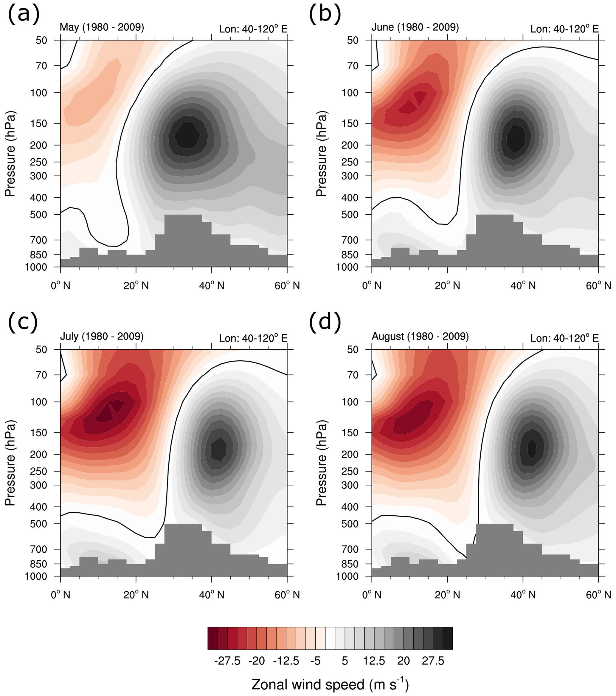
Figure 17 Zonal winds from ERA-Interim for (a) May to (d) August averaged over 1980 to 2009 and 40–120^∘ E. Red (grey) colours indicate westward (eastward) winds, and black contours indicate the zero wind line. Grey shadings mark orography.

5.3 Contribution of the TP

In this study we investigated transport from the top of the PBL to the AMA; i.e. our analyses end at the top of the PBL. Convergence of surface winds at the southern flank of the TP (Pan et al., 2016, their Fig. 8) might cause low-level transport of emissions from their source regions to the final exit and uplift region from the PBL to the AMA. As an example, emissions, for example, of CO are low over the TP (Park et al., 2009; Barret et al., 2016, their Figs. 9 and 10, respectively); nevertheless air masses transported from the PBL over the TP to the AMA can carry considerable CO signatures (Pan et al., 2016, their Figs. 2b and 7).

Independently of potential limitations in the TRJ or EMAC–ATTILA data, the increase of TP air masses to the AMA composition is also backed up by ERA-Interim data, which is shown in Fig. 17: in May the core of the subtropical jet is located right above the TP. During the course of the monsoon season, the tropical easterly jet, which is located on the southern boundary of the AMA (Dethof et al., 1999), strengthens. This indicates an increase of the anticyclonic circulation of the AMA. Further, the subtropical jet – which is located on the northern boundary of the AMA (Dethof et al., 1999) – as well as the zero wind line moves northward. Consequently, air masses that are transported upward from the TP are likely to be advected by the subtropical westerly jet during the early phase of the monsoon season (June), while they can feed into the core of the AMA during August.

Finally, as Bergman et al. (2013) found a relatively large contribution of air masses from the TP to the AMA, they discuss their results in relation to other studies that either do or do not find important contributions of the TP to the air masses (or tracer fields) in the AMA or UTLS. While they correctly argue that the results strongly depend on the chosen analysis method, we want to add that the strong intraseasonal variability might be a reason for the differences in the assessment of the TP contribution: most of the studies that find strong contributions of the TP to the AMA or UTLS focus on August conditions, for example, Fu et al. (2006), Bergman et al. (2013) and Jensen et al. (2015). In contrast, Park et al. (2009) investigated the source region contribution and transport budget of CO to the AMA and came to the conclusion that the TP has a relatively low impact on the CO maximum in the AMA region. For the source region contribution, i.e. the contribution of CO emitted from the TP, they showed that the lack of surface emissions from the TP leads to this minor impact. In a vertically resolved CO budget analysis for the TP region, they found that convection leads to a small maximum around 400 hPa, while advection leads to a negative tendency in the middle troposphere, and thus they argued that the TP does not play an important role in transport of CO to the AMA. The negative advection tendency found in their analysis is most likely related to the location of the subtropical jet over the TP in June 2005, which might have caused air masses to be transported out of the TP region. In our analyses, the contribution from the TP to air masses within the AMA increases as the subtropical jet shifts northwards from June to August, and we find that the transport of TP boundary layer air out of the AMA region decreases accordingly (see Fig. 16). Further, Devasthale and Fueglistaler (2010) put the importance of TP convection into perspective; however, they also showed that deep convective activity over the TP increases from June to August (see their Fig. 3). Similarly, from the convective upward mass flux in the EMAC–ATTILA data, we find that in July and August, the mass flux into the upper troposphere (above ∼350 hPa) over the TP is larger than in June (not shown).

6 Summary and conclusion

In this study we have analysed the transport pathways and source regions from the PBL to the AMA. This was achieved by calculating trajectories for 14 monsoon seasons using reanalysis wind fields. Additional results from 30 monsoon seasons from a Lagrangian transport model, which was run within a free-running CCM, were used to confirm these results. The presented analyses (Sects. 3 and 4) and the discussion in the previous section (Sect. 5) allow us to answer the following questions regarding the transport characteristics of air masses from the PBL to the AMA.

1. What is the climatological perspective of PBL-to-AMA transport in terms of pathways and PBL source regions? How reliable are previous results?

   • Our results show that during JJA on a climatological basis, AMA air masses come from a broad region in the PBL in Asia. With increasing height, the upward transport of air masses focuses on (the region below) the south-eastern part of the AMA. However, we found that approximately half of the PBL crossing trajectories already recirculate within the AMA considerably below 150 hPa. The attribution of the PBL source regions, however, is less clear as it is more sensitive to the modelling approach: in TRJ, the largest contributions from the named source regions are found from the TP region (around 17 %), the IND region (around 13 %) and the WP region (around 12 %). In LG-D, we find almost the same contribution from the TP (15 %) and the WP (12 %); however the contributions from IND and SEA are the largest.

2. How do the pathways and source regions vary on intraseasonal and interannual timescales?

   • We find that the qualitative behaviour of the transport pathways is similar throughout the monsoon season and between different monsoon seasons, i.e. upward transport on the south-eastern side below the AMA and subsequent transport within the AMA. Nevertheless, in particular concerning the intraseasonal variation, the transport pathways shift considerably northwards over the course of the monsoon season in accordance with the shift of the monsoon system. Further, we also find strong interannual and intraseasonal variability of the PBL source region contributions. For the latter, the contribution from the TP, which strongly increases from around 2 % (4 %) in TRJ (LG-D) in early June to around 24 % (20 %) in TRJ (LG-D) in early August, sticks out. This increase is (partly) related to the relative position of the AMA and the subtropical jet. We show that taking the strong intraseasonal variability into account can help to reconcile differences in previous studies concerning PBL-to-AMA transport, in particular concerning the contribution of the TP.

3. Are the PBL source regions and the transport pathways sensitive to interannual east–west shifts of the AMA?

   • We identify shifts in the transport pathways between east and west years, although the main characteristics are qualitatively unchanged. Further, we show that the longitudinal shifts of the AMA are related to the so-called monsoon Hadley index. For the PBL sources, we find no considerable differences between east and west years for the defined source regions, while a map shows that there are (small) regional shifts in the contribution of the PBL sources.

From our results, we find that the three-dimensional pathways of trajectories give a conclusive picture of transport from the PBL to the AMA. However, the relative contribution from the PBL source regions are (except for TP and WP) less robust. In our analysis we could not distinguish whether the differences in source region contribution are a result of the different synoptic conditions in the free-running EMAC–ATTILA simulation compared to the reanalysis-driven TRJ calculations or actually a result of the consideration of Lagrangian convection in the EMAC–ATTILA data. A first indication of faster vertical transport due to parametrized convection in the LG data comes from the observation that a lower fraction of trajectories do not encounter the PBL in the LG simulations compared to the TRJ data.

To allow for a more robust picture of the transport from the PBL to the AMA in the monsoon region, further investigations with various model setups would be beneficial. In particular, a set of tailored simulations with and without convective transport would be valuable to assess the impact of convective transport on the individual source region contributions to AMA air masses.

Appendix A

A1 AMA boundary determination

In this study, mostly trajectories starting within the core of the AMA have been analysed. The determination of the boundary of the AMA is difficult, and many studies have used various quantities and thresholds to determine the boundary of the AMA (e.g. Park et al., 2007; Garny and Randel, 2013; Ploeger et al., 2015; Santee et al., 2017). Here, the boundary determination is based on a geopotential height anomaly (GPHA) threshold, as proposed by Barret et al. (2016). They calculated GPHAs with respect to the 50^∘ S–50^∘ N mean and used a threshold of 270 m for the pressure levels 100, 150 and 200 hPa based on previously used boundaries. For our data, we have derived thresholds explicitly for the trajectory model calculations using ERA-Interim data at 2.5^∘ grid spacing and for the EMAC–ATTILA simulations using the CCM grid point data. In principal, we have determined suitable threshold candidates by deriving a single GPHA value, which on average represents the strongest anticyclonic circulation. This was done by calculating the mean of the GPHA values associated with the strongest meridional winds (southward and northward) along the ridge line (see Zhang et al., 2002, for the ridge line). For EMAC–ATTILA, we further required the maximum wind speed to be located at a grid point with GPHA of at least 100 m to avoid noise from unrealistically low values. Using this technique, we determined anomaly thresholds of 280 and 295 m for ERA-Interim and EMAC–ATTILA data, respectively. The value of 280 m for ERA-Interim is in good agreement with the threshold of 270 m used by Barret et al. (2016).

A2 Selection of summer seasons for the TRJ calculations

The trajectory model calculations described in Sect. 2 have been performed for 14 NH summer seasons in the period 1979–2013. These NH summers have been selected as the mean position of the AMA was rather displaced to the east or west. For the selection a modified version of the South Asian High Index (SAHI), which was originally defined by Wei et al. (2014), has been used. Wei et al. (2014) calculated the SAHI by standardizing the time series of differences of geopotential height over a box in the east of the AMA (22.5–32.5^∘ N ×85–105^∘ E) minus that over a box in the west of the AMA (22.5–32.5^∘ N ×55–75^∘ E) at a single pressure level. Compared to the definition by Wei et al. (2014), we use a modified version, which standardizes the sums of these differences over three pressure levels (100, 150 and 200 hPa) to better capture the 3D structure of the AMA. Further, we use these pressure levels as they are centred around the starting level of the trajectories (150 hPa). ERA-Interim data with a grid spacing of $\mathrm{2.5}{}^{\circ }\times \mathrm{2.5}{}^{\circ }$ have been used to determine the modified SAHI, and using a threshold of $\pm \mathrm{0}.$7 deviation from the mean, we found 14 years with a rather eastward or westward displaced AMA (7 years each³). The corresponding starting probabilities for the east (cyan) and west (magenta) composites are shown in Fig. 2.

Appendix B: Supporting figures

Figure B1 Starting frequency of trajectories for LG-D (a) and LG-K (b) over the years 1981–2010. For LG-K, data for 2008 were removed; see text for details.

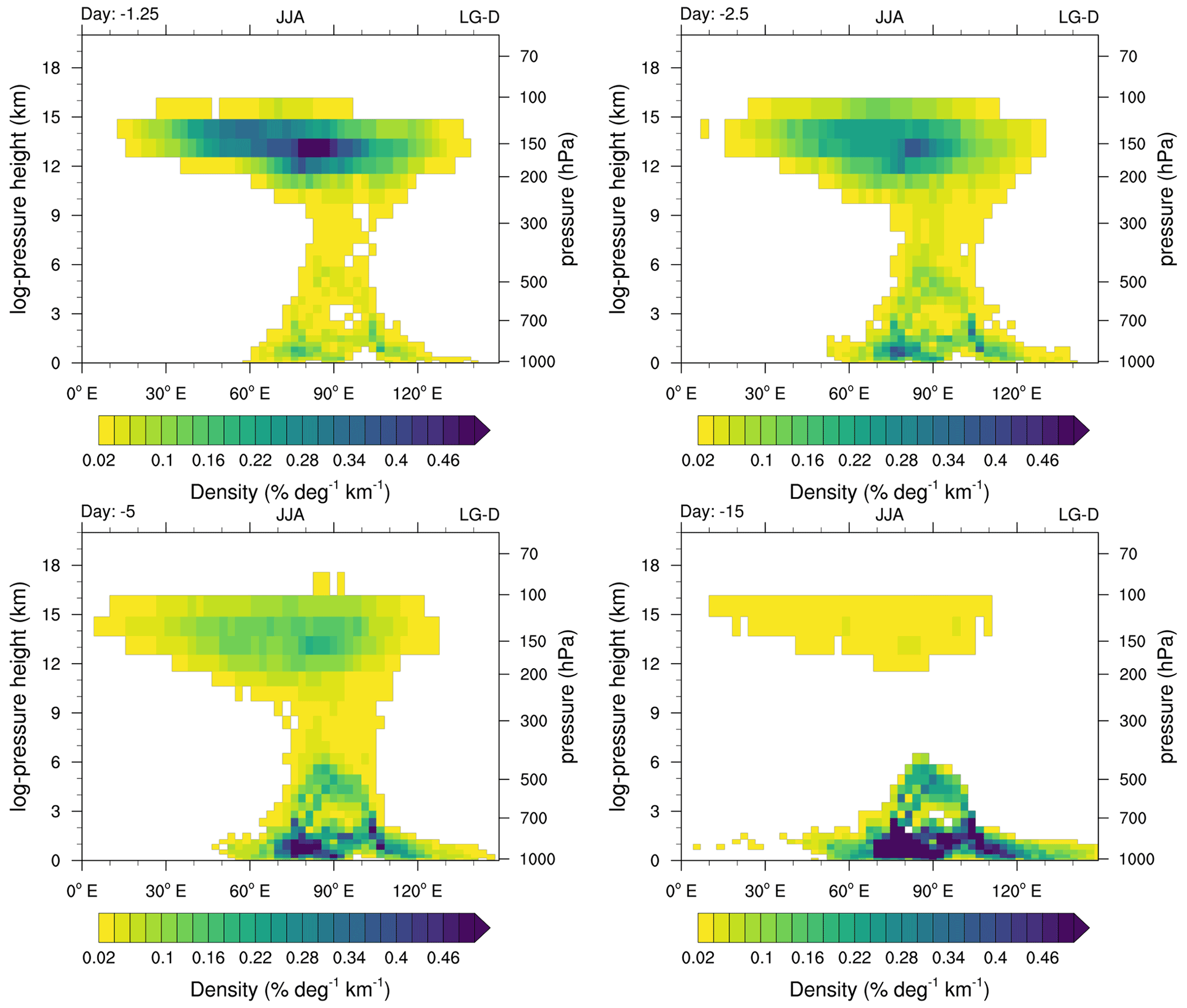
Figure B2 Density of trajectory distributions integrated over 0–50^∘ N as in Fig. 5 but for the LG-D data from 1981–2010 for 1.25, 2.5, 5 and 15 d prior to the arrival of the trajectories in the AMA at approximately 150 hPa.

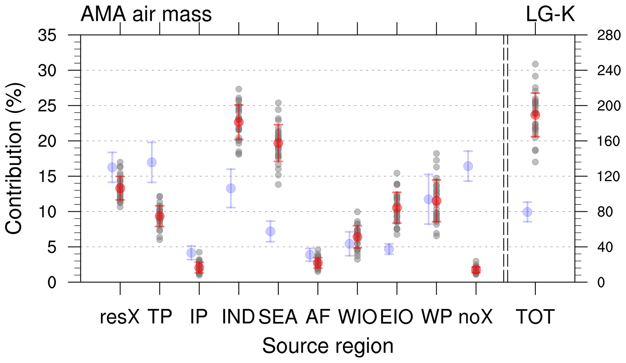
Figure B3 Contributions of PBL sources to the AMA around 150 hPa for the LG-K simulation for 1981–2010 (with 2008 removed; see text for details). Mean values are given as red dots, red whiskers denote the interannual standard deviation and individual years are indicated as grey dots. For TOT the right axis denotes the total number of trajectories in units of 10³ trajectories. For comparison, faint blue dots and whiskers denote the values from the TRJ data.

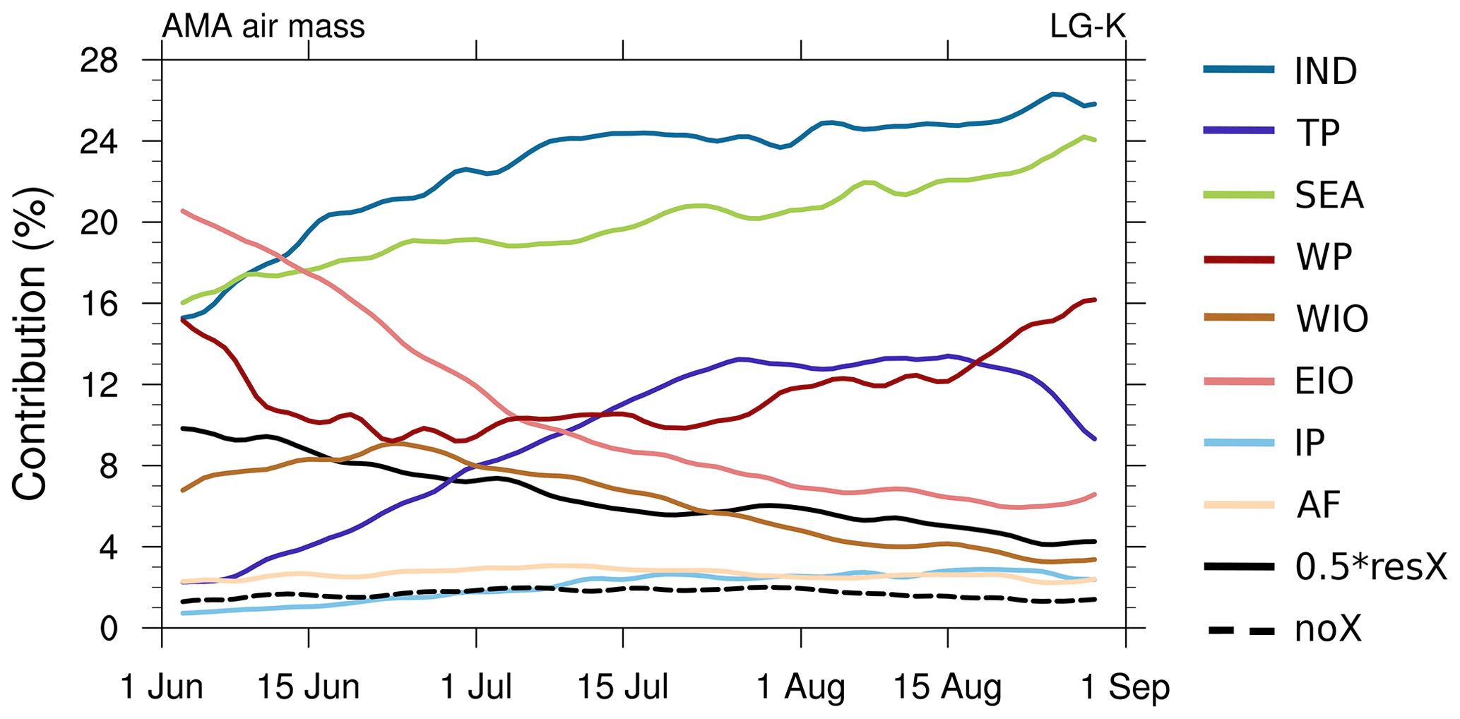
Figure B4 Source evolution in the LG-K data during 1981 to 2010 (with 2008 removed; see text for details). resX data have been scaled by 0.5. All contributions have been smoothed using 5 d running means (weights of $\left[\frac{\mathrm{1}}{\mathrm{9}},\frac{\mathrm{2}}{\mathrm{9}},\frac{\mathrm{3}}{\mathrm{9}},\frac{\mathrm{2}}{\mathrm{9}},\frac{\mathrm{1}}{\mathrm{9}}\right]$), while daily data were produced from summing up the 10-hourly data for each day.