The climate impact of hydrogen-powered hypersonic transport

Hypersonic aircraft flying at Mach 5 to 8 are a means for traveling very long distances in extremely short times and are even significantly faster than supersonic transport (Mach 1.5 to 2.5). Fueled with liquid hydrogen (LH2), their emissions consist of water vapor (H₂O), nitrogen oxides (NO_x), and unburned hydrogen. If LH2 is produced in a climate- and carbon-neutral manner, carbon dioxide does not have to be included when calculating the climate footprint. H₂O that is emitted near the surface has a very short residence time (hours) and thereby no considerable climate impact. Super- and hypersonic aviation emit at very high altitudes (15 to 35 km), and H₂O residence times increase with altitude from months to several years, with large latitudinal variations. Therefore, emitted H₂O has a substantial impact on climate via high altitude H₂O changes. Since the (photo-)chemical lifetime of H₂O largely decreases at altitudes above 30 km via the reaction with O(¹D) and via photolysis, the question is whether the H₂O climate impact from hypersonics flying above 30 km becomes smaller with higher cruise altitude. Here, we use two state-of-the-art chemistry–climate models and a climate response model to investigate atmospheric changes and respective climate impacts as a result of two potential hypersonic fleets flying at 26 and 35 km, respectively. We show, for the first time, that the (photo-)chemical H₂O depletion of H₂O emissions at these altitudes is overcompensated by a recombination of hydroxyl radicals to H₂O and an enhanced methane and nitric acid depletion. These processes lead to an increase in H₂O concentrations compared to a case with no emissions from hypersonic aircraft. This results in a steady increase with altitude of the H₂O perturbation lifetime of up to 4.4±0.2 years at 35 km. We find a 18.2±2.8 and 36.9±3.4 mW m⁻² increase in stratosphere-adjusted radiative forcing due to the two hypersonic fleets flying at 26 and 35 km, respectively. On average, ozone changes contribute 8 %–22 %, and water vapor changes contribute 78 %–92 % to the warming. Our calculations show that the climate impact, i.e., mean surface temperature change derived from the stratosphere-adjusted radiative forcing, of hypersonic transport is estimated to be roughly 8–20 times larger than a subsonic reference aircraft with the same transport volume (revenue passenger kilometers) and that the main contribution stems from H₂O.

1 Introduction

The climate impact of aircraft emissions has been studied for decades and becomes more and more important. Estimated aviation growth rates will increase aviation's contribution to climate change and, by that, challenge the support of the Paris Climate Agreement (UN, 2015; Terrenoire et al., 2019; Grewe et al., 2021; Planès et al., 2021). A recent study estimates the contribution of aircraft activity to human-made climate change to be 3.5 (3.4, 4.0) %, which is an estimate based on effective radiative forcing and aviation fuel use (2011) (Lee et al., 2021). Furthermore, while carbon dioxide (CO₂) effects contribute one-third to the effective radiative forcing, non-CO₂ effects contribute two-thirds. This estimate is based on current aircraft fleets that are powered with kerosene and fly at altitudes from 10 to 12 km. With these aircraft, it takes travelers approximately one day to fly around the world.

Two development goals for future aircraft fleets are, on the one hand, to reduce climate impact and, on the other hand, to reduce travel time. As an example, roadmaps for a more climate-friendly, liquid-hydrogen-based aviation industry have been developed in agreement with existing research, estimating the potential reduction in climate impact to be 50 %–75 % (Fuel Cells and Hydrogen: Joint Undertaking, 2020). However, this mainly addresses the concept of subsonic aircraft flying at altitudes of 10–12 km. Higher altitudes are especially interesting for high-speed aircraft concepts that promise to save a considerable amount of travel time for customers, especially on middle- and long-range flights. Aircraft designs in that category are super- and hypersonic aircraft. These aircraft are designed to travel at higher speeds and higher altitudes compared to conventional subsonic aircraft and could reduce travel time around the globe to some hours. In turn, however, flight altitude and fuel type, which depend on aircraft design, can have a strong influence on atmospheric composition and thus on climate impact. The climate impact of high-speed aircraft designs has been addressed for supersonic aircraft flying with kerosene as well as with cryogenic fuels in the lower stratosphere (IPCC, 1999; Gauss et al., 2003; Grewe et al., 2007, 2010).

The impact of supersonic aircraft at stratospheric altitudes is often discussed in terms of ozone concentration changes and ultraviolet radiation, and extensive overviews on these topics have recently been published (Zhang et al., 2021; Tuck, 2021; Matthes et al., 2022). The first notes indicating that NO_x from supersonics might significantly affect the ozone layer were published in the 1970s (Crutzen, 1970, 1972; Johnston, 1971). Additionally, there are multiple publications on the quantitative climate impact of supersonic aircraft fleets. A review of a selection of research programs, including a direct comparison of radiative forcings (RF), was given by Grewe et al. (2010), who estimated the ratio of RF from supersonic to subsonic aircraft to be 3 (S4TA fleet, eight passengers), 6 (Airbus fleet, 250 passengers, Grewe et al., 2007), and 14 (Boeing fleet, 309 passengers, IPCC, 1999). While these numbers initially appear to differ greatly, the authors present a correlation of flight altitude (range from 15–20 km) and RF of non-CO₂ effects and additionally state that supersonic climate impact can be scaled approximately with fuel consumption. Hence, cruise altitude (i.e., speed, which in turn influences fuel consumption) is clearly a crucial factor for climate impact.

At even higher altitudes, in the middle to upper stratosphere, hypersonic aircraft travel at Mach 4 or more, and the emitted trace gases react in another atmospheric environment compared to sub- and supersonic aircraft. Depending on the cruise altitude and latitude of potential routes, hypersonic aircraft could fly in the upper parts of or above the ozone layer. As reference, the ozone (O₃) mixing ratio is largest at around 31 km at tropical regions and has no clear peak at polar regions (Tegtmeier et al., 2013). The middle atmospheric balance of water vapor is determined by methane oxidation, photochemical lifetimes of HO_x compounds, and upward transport through the tropical upper troposphere–lower stratosphere (UTLS), which is limited by the cold temperatures (Brasseur and Solomon, 2005; Frank et al., 2018; le Texier et al., 1988). Polar dehydration caused by the sedimentation of polar stratospheric cloud particles contributes to the balance. The climate impact of hypersonic aircraft emissions largely depends on their atmospheric residence time. More specifically, the residence time of species emitted by aircraft in the stratosphere is mainly controlled by the large-scale circulation of air (Brewer–Dobson circulation), their chemical interaction with stratospheric air constituents, and photolysis. All three processes are highly dependent on altitude. The amount of emitted species is determined by aircraft and engine design, fuel type, and trajectory layout. Kerosene, as the conventional fuel, is a technical option for hypersonic aircraft, but the initial focus in hypersonic studies is often on cryogenic aircraft. In general, cryogenic aircraft can be powered by pure gases, such as methane (CH₄) or hydrogen (H₂), that are cooled to the liquid phase with the goal of reducing volume – i.e., increasing range per tank fill – and for other technical advantages (Peschka, 1998). Hence, compared to kerosene, cryogenic fuel could, in theory, be particle free and would not have an indirect aerosol effect (Ponater et al., 2006). One of the few potential cryogenic fuels is liquid natural gas (LNG), which consists mostly of CH₄. Similar to kerosene-fueled aircraft, LNG ultimately increases atmospheric CO₂ concentrations. In comparison to H₂ fuel, LNG's direct climate impact could be slightly lower at specific altitudes (cruise altitude of approximately 13 km; Grewe et al., 2017). However, the CO₂ perturbation originating from fossil fuels is subject to a large variety of sinks with different lifetimes. In general, the range is approximated to be 2–20 centuries, where most of the CO₂ is taken up by ocean and biosphere sinks, with 20 %–35 % remaining in the atmosphere for a longer time. Hence, released CO₂ will affect climate for tens of thousands to hundreds of thousands of years (Archer and Brovkin, 2008; Archer et al., 2009). On the other hand, H₂-fueled aircraft mainly emit water vapor (H₂O), whereas nitrogen oxides (NO_x) and H₂ are byproducts, with the latter depending on combustion efficiency. Their lifetimes are hours to years for H₂O and years for NO_x and H₂ (Brasseur and Solomon, 2005; Johnston et al., 1989; Grewe and Stenke, 2008; Ehhalt and Rohrer, 2009), which is substantially lower than for CO₂. Hence, a lifetime at least 1 order of magnitude shorter is a reason why, currently, H₂ fuel is often the preferred climate-friendly option for hypersonic aircraft designs. Another reason is the potentially more efficient (photo-)chemical destruction of H₂O at high altitudes, reducing the residence time and thus climate impact of emitted H₂O. More specifically, several studies suggest that the chemical reaction of H₂O with O(¹D) and photolysis could efficiently remove emitted H₂O at upper stratospheric altitudes and higher (Brasseur and Solomon, 2005; Steelant et al., 2015). This could potentially create a synergy of aircraft flying at these altitudes and H₂ propulsion aimed at reducing climate impacts. Thus, hypersonic aircraft with H₂ propulsion are seen as a potentially more climate-friendly alternative to supersonic aircraft. For completeness, it is important to mention that the choice of fuel type does not only include climate impact but is also a trade-off between, for example, energy content – i.e., best range of aircraft – or cooling properties for thermal regulation (Blanvillain and Gallic, 2015).

However, the quantitative climate impact of hypersonic aircraft, regardless of fuel type, has not yet been assessed with a global atmospheric model, and how it compares to supersonic aircraft still remains to be answered. In particular, H₂-fueled aircraft are important to look at due to the broad discussions about global H₂ infrastructure and in consideration of the fact that H₂O is a potent greenhouse gas that affects the ozone at stratospheric altitudes (Stenke and Grewe, 2005). Recent publications on the impact on atmospheric composition by hypersonic aircraft are few and focus on H₂-fueled aircraft. Ingenito (2018) published an estimate based on a fleet of 200 aircraft of type LAPCAT II MR2.4 (Steelant and Langener, 2014, Long-Term Advanced Propulsion Concepts and Technologies) flying at 30 km altitude, quantifying the reduction of atmospheric ozone with $\mathrm{3.6}\times {\mathrm{10}}^{-\mathrm{4}}$ % and a temperature increase due to H₂O to 142 mK in one year. Another study by Kinnison et al. (2020) was done with a global atmospheric model to assess the impact of hypersonic fleet emissions on the ozone layer at altitudes of 30 and 40 km. They focus on the sensitivity of stratospheric ozone to local perturbations of NO_x and H₂O. Their estimate for a reduction of atmospheric ozone with the same amount of fuel is 4.0 % and 2.2 % at 30 and 40 km, respectively.

In this study, we evaluate the climate impact of non-CO₂ effects from hypersonic aircraft and its altitude dependency with the metric of stratosphere-adjusted RF. In particular, we present the impact of H₂O, NO_x, and H₂ emissions from hypersonic aircraft driven with H₂ fuel on atmospheric composition and briefly discuss the change in UV radiation. The results are based on the comparison of simulations with two chemistry–climate models. The hypersonic emission data this study uses were developed in the “HIgh speed Key technologies for future Air transport – Research & Innovation cooperation scheme” project (HIKARI, Blanvillain and Gallic, 2015), whose authors recommend H₂ fuel as a first choice. The economic and technical requirements of two fleets of hypersonic aircraft considered there will provide the estimate of the altitude dependency of the climate impact of hypersonic aircraft emissions. Two advanced hypersonic fleet scenarios (Technology Readiness Level 1–3) – differing in cruise altitude, cruise speed, and thus fuel consumption – will allow the comparison of the climate impacts of technically viable hypersonic aircraft concepts. The two hypersonic aircraft designs considered here are the models ZEHST (Zero Emission High-Speed Transport) and LAPCAT PREPHA (Programme de REcherche et de technologie sur la Propulsion Hypersonique Avancée, Falempin et al., 1998; Scherrer et al., 2016), with cruise altitudes at approximately 26 and 35 km, respectively. The paper is structured as follows. After the introduction, we present the two chemistry–climate models EMAC (ECHAM/MESSy; European Centre HAMburg general circulation model; Modular Earth Submodel System) and LMDZ-INCA (Laboratoire de Météorologie Dynamique; INteraction with Chemistry and Aerosols) and their setups. In Sect. 3 we present the HIKARI emission inventory and the temporal evolution of aircraft emissions. After a model evaluation with aircraft measurements in Sect. 4, we show the atmospheric composition changes in Sect. 5. The climate impact is part of Sect. 6, “Radiation and climate”. In the end, a discussion and summary is included.

2 Methods and simulations

We have performed simulations of atmospheric changes caused by emissions from hypersonic transport with the two atmospheric chemistry general circulation models (AC-GCMs) EMAC and LMDZ-INCA in order to address model dependencies of the results. The differences and conformity between model setups that were used in this study are presented in Table 1. It lists the key properties of both models. EMAC consists of the spectral dynamical core of the GCM ECHAM5 by the Max Planck Institute for Meteorology (version five, Roeckner et al., 2006) and MESSy, able to combine all components relevant for Earth System Models, as published by Jöckel et al. (2005, 2010, 2016).

The LMDZ-INCA global chemistry–aerosol–climate model couples on-line the LMDZ general circulation model (version six, Hourdin et al., 2020) and the INCA model (version five, Hauglustaine et al., 2004, 2014). The interaction between the atmosphere and the land surface is ensured through the coupling of LMDZ with the ORCHIDEE (Organizing Carbon and Hydrology In Dynamic Ecosystems, version 1.9) dynamical vegetation model (Krinner et al., 2005). More information on the model setups are presented in the following sub-chapters.

Table 1 Table stating the key properties of the model setups for EMAC and LMDZ-INCA, as applied for this study.

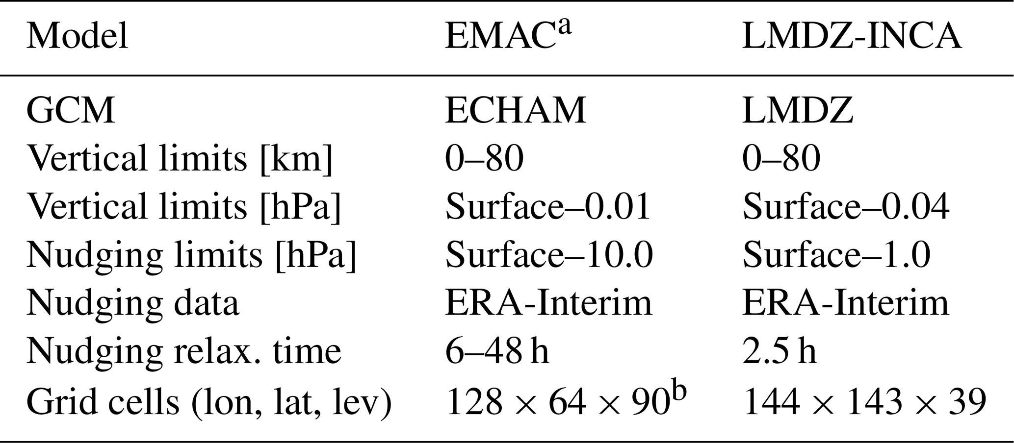
^a ECHAM5 v5.3.02, MESSy v2.54.0, Jöckel et al. (2010). ^b Named T42L90MA, where T42 refers to a triangular truncation at wave number 42, corresponding to a quadratic Gaussian grid of approximately 2.8^∘ by 2.8^∘ in latitude and longitude; L90 refers to 90 vertical hybrid pressure levels and MA to “middle atmosphere”.

While the model setups of EMAC and LMDZ-INCA are consistent with respect to the model domain and nudging data, there are differences with respect to the vertical resolution, the nudging relaxation time, and the model domain where nudging is applied. Both models were intensively validated, e.g., the dynamics at stratospheric altitudes by the model's stratospheric age of air and by tropical upward mass flux. Further details on the respective models are given in the following subsections.

2.1 EMAC model setup

The EMAC model setup is based on that of simulation RC1SD-base-10, recommended due to its affirmative agreement with observations, especially ozone, and described in detail by Jöckel et al. (2016). The vertical resolution of the 90 hybrid model layers in EMAC is approximately 550 m in the UTLS region, reaches 1200 m at the stratopause, and increases to 3200 m in the middle atmosphere The model results were compared extensively with ERA-Interim. Deviations from model to observations are a cold bias, with a vertical maximum at 200 hPa and values of ±4 K (Fig. 12, Jöckel et al., 2016). A comparison with satellite data shows that, over the annual cycle, ozone volume mixing ratios are well reproduced in the stratosphere, apart from southern polar regions, and with larger differences at tropospheric altitudes. The stratospheric southern polar bias is larger in free-running EMAC simulations and are especially low in simulations with specified dynamics (without mean temperature nudging). Hence, our chosen EMAC model setup is especially well suited for our application of modeling stratospheric ozone. An IAGOS-CARIBIC (In-service Aircraft for a Global Observing System; Civil Aircraft for the Regular Investigation of the atmosphere Based on an Instrument Container: Petzold et al., 2015) data comparison for the UTLS shows deviations around 5 % and larger values up to 30 % in June–September for regions above the tropopause and an overestimate of up to 40 % in the troposphere. Methane, carbon monoxide, and acetone concentrations are underestimated by the model, specifically at tropospheric altitudes. Transport by the Brewer–Dobson circulation was tested by comparing the model tropical upward mass flux to ERA-Interim and the mean age of stratospheric air (AoA) to MIPAS (Michelson Interferometer for Passive Atmospheric Sounding) observations. While the largest differences for AoA are at polar latitudes and the upper stratosphere, the model still shows a reasonable agreement overall, especially for the lower stratosphere and extratropics, and the tropical upward mass flux shows the best agreement for setups with specified dynamics (nudging) and without global mean temperature nudging (Jöckel et al., 2016). In summary, while there are deviations, the setup including nudging is, amongst others, especially well suited for stratospheric sensitivity studies.

As this study assesses the impact of emitted H₂O (as well as NO_x and H₂), a decoupling of atmospheric dynamic chemistry and radiation was technically not possible when adding H₂O to the model's hydrological cycle. However, we achieved a sufficiently large signal-to-noise ratio by Newtonian relaxation (nudging) towards ERA-Interim reanalysis data for the years 2000–2014. EMAC is based on the spectral transform dynamical core of ECHAM. The nudging is applied by Newtonian relaxation of the prognostic variables of divergence, vorticity, and temperature as well as the logarithm of the surface pressure in the spectral representation (spherical harmonics) of these variables towards the ECMWF (European Centre for Medium-Range Weather Forecasts) ERA-5 reanalysis data (Dee et al., 2011). u and v wind are derived variables calculated through derivation and spectral transformation. The wave 0 of temperature (global mean) is omitted; furthermore, there is no nudging applied on the sub-synoptic scale, aiming at an optimal compromise between observed (i.e., reanalyzed) and simulated meteorology. Moreover, the nudging is applied in a vertical direction only between the fourth model layer above the ground and approximately 200 hPa in order to avoid inconsistencies in the planetary boundary layer and to let the stratosphere develop freely, driven by the tropospheric wave activity. This nudging setup is identical to that of the RC1SD-base-10 simulation described by Jöckel et al. (2016). The ECMWF ERA-5 reanalysis data are preprocessed by spectral transformation and truncation for the applied model resolution. The respective relaxation times are listed in Table 1. Further information on the very similar nudging process, apart from different relaxation times, is described in the next subsection about LMDZ-INCA. Prognostic variables were accounted for by the MESSy submodel TENDENCY to tag submodel contributions – such as cloud, advection, or emission processes – to specific humidity (Eichinger and Jöckel, 2014). Additionally, H₂O emissions were added to the model's hydrological cycle with a new MESSy submodel (H2OEMIS), which uses either TENDENCY (in this study) or directly adds water vapor perturbations to the specific humidity tracer. An overview of all active submodels can be found in the Appendix.

2.1.1 ECHAM5/MESSy submodel H2OEMIS

H₂O and the associated hydrological cycle play an important role in atmospheric radiation and dynamics and, thereby, the general circulation. As it is a precursor of the atmospheric hydroxyl radical (OH), it also largely controls atmospheric chemistry. For earlier versions of the model, the chemistry calculations were operated with an H₂O tracer that had to be kept synchronous with the prognostic specific humidity of the underlying GCM. In recent versions, the chemistry feedback on the hydrological cycle now directly alters the specific humidity. Due to this, it was not possible to include offline H₂O to alter the prognostic specific humidity directly. But the modular structure easily allowed the development of the new submodel H2OEMIS to include the possibility of directly emitting H₂O into the atmosphere and altering specific humidity. Briefly summarized, gridded H₂O emission flux data is imported into the model via the IMPORT submodel (Kerkweg and Jöckel, 2015); then H2OEMIS converts the flux into a tendency of the specific humidity and applies this tendency to the prognostic variable qm1, i.e., specific humidity in MESSy. The submodel and further information are available with the MESSy release version 2.55.0 (https://www.messy-interface.org/, last access: 31 August 2022). Two short movies can be found in the video supplements showing H₂O emitted by hypersonic aircraft and its addition to the specific humidity (zonal mean representation and world map view, respectively).

2.1.2 Additional diagnosis of chemical destruction and production of H₂O with MECCA

The net amount of chemical production and destruction of H₂O is significant for the concentration of H₂O in the stratosphere. Above 20 km, the largest contribution comes from transport through the tropical tropopause layer via the deep branch of the Brewer–Dobson circulation and oxidation of CH₄, which was recently reconfirmed with EMAC model studies by Eichinger et al. (2015a, b) and Frank et al. (2018) and through satellite studies by Noël et al. (2018). In EMAC, the chemical mechanism is applied, among others, via the MESSy submodel MECCA (Module Efficiently Calculating the Chemistry of the Atmosphere), developed by Sander et al. (2005, 2011). This specific submodel is able to include tracers that keep track of the production as well as the destruction of chemical reactants. Thus, we included five tracers for the chemical destruction of H₂O and 45 tracers for the chemical production of H₂O for a deeper understanding of the underlying processes. Further information on the H₂O-specific reaction rates and all other reaction rates are given in the supplement of this study (file meccanism.pdf, scavinism.pdf) and beyond that in the supplement of Jöckel et al. (2016). While MECCA considers gas- and heterogeneous-phase reactions in the tropo- and stratosphere, the submodel SCAV (SCAVenging) includes aqueous phase reactions in clouds and precipitation and the corresponding induced removal of trace gases and aerosols by wet deposition (Tost et al., 2006); CH₄ (Winterstein and Jöckel, 2021) issues CH₄ oxidation (while MECCA accounts for the resulting water vapour from methane oxidation and feeds it back to specific humidity); MSBM (multiphase stratospheric box model) calculates the polar stratospheric cloud chemistry (Jöckel et al., 2010); DDEP (dry deposition) and SEDI (SEDImentation) are responsible for dry deposition and sedimentation of aerosols, respectively (Kerkweg et al., 2006a); AIRSEA addresses air and ocean surface interaction (Pozzer et al., 2006); OFFEMIS (offline emissions) and ONEMIS (online emissions) add prescribed and online-calculated emissions (Kerkweg et al., 2006b); and LNOX (lightning nitrogen oxides) includes NO_x production by lightning, where we used the “Grewe” coupling parameterization, as described in Tost et al. (2007) and Grewe et al. (2001), which is based on convective mass flux. The resulting total lightning NO_x for the baseline simulation is 5.0 TgN yr⁻¹.

2.2 LMDZ-INCA model setup

In the present LMDZ-INCA configuration, we use the “standard physics” parameterization of the GCM (Boucher et al., 2020). The model includes 39 hybrid vertical levels extending from the surface up to 80 km. The vertical resolution of LMDZ-INCA in the applied resolution is approximately 1000–1300 m in the UTLS region, reaches 5000 m at the stratopause, and increases to 8700 m in the mesosphere. The horizontal resolution is 1.9^∘ in latitude and 3.75^∘ in longitude. The primitive equations in the GCM are solved with a 3 min time step, large-scale transport of tracers is carried out every 15 min, and physical and chemical processes are calculated at a 30 min time interval. For a more detailed description and an extended evaluation of the GCM, we refer to Hourdin et al. (2020). The large-scale advection of tracers is calculated based on a monotonic, finite-volume second-order scheme (Hourdin and Armengaud, 1999). Deep convection is parameterized according to the scheme of Emanuel (1991). The turbulent mixing in the planetary boundary layer is based on a local second-order closure formalism. The transport and mixing of tracers in the LMDZ-GCM have been investigated and evaluated against observations for both inert tracers and radioactive tracers (e.g., Hourdin and Issartel, 2000; Hauglustaine et al., 2004) and in the framework of inverse modeling studies (e.g., Bousquet et al., 2010; Zhao et al., 2019).

INCA initially included a state-of-the-art CH₄–NO_x–CO–NMHC–O₃ tropospheric photochemistry (Hauglustaine et al., 2004; Folberth et al., 2006). The tropospheric photochemistry and aerosols scheme used in this model version is described through a total of 123 tracers, including 22 tracers to represent aerosols. The model includes 234 homogeneous chemical reactions, 43 photolytic reactions, and 30 heterogeneous reactions. Please refer to Hauglustaine et al. (2004) and Folberth et al. (2006) for the list of reactions included in the tropospheric chemistry scheme. The gas-phase version of the model has been extensively compared to observations in the lower troposphere and in the upper troposphere. For aerosols, the INCA model simulates the distribution of aerosols with anthropogenic sources, such as sulfates, nitrates, black carbon (BC), and organic carbon (OC) as well as natural aerosols such as sea salt and dust. The aerosol component of the LMDZ-INCA model has been extensively evaluated during the various phases of AEROCOM (e.g., Gliss et al., 2021; Bian et al., 2017).

Earlier versions of the LMDZ-INCA, model including gas-phase tropospheric chemistry, have only been used previously to assess the impact of subsonic aircraft on tropospheric ozone (Koffi et al., 2010; Hauglustaine and Koffi, 2012). This version of the model has been extended to include an interactive chemistry in the stratosphere and mesosphere (Terrenoire et al., 2022). Chemical species and reactions specific to the middle atmosphere have been included in the model. A total of 31 species – mostly belonging to the chlorine and bromine chemistry – as well as 66 gas phase reactions and 26 photolytic reactions were added to the standard chemical scheme. Water vapor is now affected by both physical and chemical processes in LMDZ. In the stratosphere, an additional tracer is introduced in order to account for photochemical production and destruction in INCA. In addition, heterogeneous processes on polar stratospheric clouds (PSCs) and stratospheric aerosols are parameterized in INCA following the scheme implemented by Lefevre et al. (1994). The excess of H₂O and HNO₃ is removed from the gas phase when saturation occurs and is used to compute the surface area concentration in the PSC region. Heterogeneous reaction rates are calculated explicitly as a function of the surface area available, mean molecular velocity, and the reaction probabilities. The model does distinguish between liquid nitric acid trihydrate (NAT, HNO₃ ⋅ 3 H₂O), liquid supercooled ternary solutions (STS, HNO₃ ⋅ H₂SO₄ ⋅ H₂O), and solid ice PSCs. Furthermore, the PSC scheme includes sedimentation of the PSC particles, which affects the vertical distribution H₂O, HNO₃, and HCl. Condensed species are returned to the gas phase when clouds evaporate. In the presence of PSCs, the heterogeneous reactions convert bromine and chlorine reservoirs (HCl, HBr, ClONO₂, BrONO₂) into reactive species (Cl₂, ClNO₂, HOCl, Br₂, BrNO₂, HOBr) based on nine additional heterogeneous reactions introduced in the chemical scheme. The distribution of stratospheric aerosols is prescribed according to the CCMI exercise (Chemistry–Climate Model Initiative; Thomason et al., 2018).

In this study, meteorological data from the European Center for Medium-Range Weather Forecasts (ECMWF) ERA-Interim reanalysis have been used to nudge the GCM winds from 1000 to 1 hPa. These GCM winds are interpolated on the horizontal grid before the simulation runs and are interpolated on the model pressure levels at each time step. The relaxation of the GCM winds towards ECMWF meteorology is performed by applying a correction term to the GCM u and v wind components at each time step, with a relaxation time of 2.5 h (Hourdin and Issartel, 2000; Hauglustaine et al., 2004). The ECMWF fields are provided every 6 h and are interpolated onto the LMDZ grid.

The anthropogenic emissions from the Shared Socioeconomic Pathways scenarios (SSPs) (scenario SSP3-7.0) prepared by Gidden et al. (2019) are used and added to the natural fluxes used in the INCA model. The ORCHIDEE vegetation model has been used to calculate offline the biogenic surface fluxes of isoprene, terpenes, acetone, and methanol as well as NO soil emissions, as described by Lathière et al. (2006). The lightning NO_x emissions are parameterized in the model based on convective cloud heights, as described in Jourdain et al. (2001). Based on this parameterization, the total lightning NO_x emissions for the baseline simulation are 5.5 TgN yr⁻¹.

2.3 Simulations

Both models simulate a time period of 15 years. This includes a 10 to 12 year spin-up phase to achieve a chemical and dynamic equilibrium that takes into account the long lifetimes of trace gases in the stratosphere. Lower boundary conditions as well as direct and traffic emissions of simulations are based on IPCC's (Intergovernmental Panel on Climate Change) RCP6.0 (Relative Concentration Pathway) scenario (CCMI) for EMAC and the SSP3-7.0 (Shared Socioeconomic Pathways) scenario for LMDZ-INCA. This includes the surface mixing ratios for methane and nitrous oxide as well as for chlorine- and bromine-containing species and excludes air traffic, where we used an emission inventory from the HIKARI project. The RCP6.0 and SSP3-7.0 scenarios are very similar, and the latter can be treated as an updated version (from the Coupled Model Intercomparison Project (CMIP) Phase 6) of the former (from CMIP Phase 5). The beginning of the air fleet operation including hypersonic aircraft was set to 2050. Therefore, the assumptions of the RCP scenario for other emissions are the 15 year period 2050–2064. The assumptions of SSP are fixed on their 2050 values. In summary, on the one hand, the simulations were carried out with nudged dynamics, allowing a reduction of the signal-to-noise ratio for the time period 2000–2014; on the other hand, the atmosphere's chemical composition of simulations is based on assumptions from 2050 (and onwards), i.e., when hypersonic aircraft technology is potentially ready for commercial use.

3 The HIKARI emission inventory and spin up

3.1 Emission

HIKARI was an international project of Europe and Japan for high-speed transport, resulting in a potential timeline for further development of high-speed transportation up to commercial operation (hikari means “light” in Japanese, CORDIS: EU research results, 2015). Blanvillain and Gallic (2015) published the roadmap study in 2015, which combines economic viability, environmental constraints, and technological requirements. We use the formerly unpublished trade-off emission scenarios by HIKARI. These include two hypersonic scenarios with the aircraft ZEHST and LAPCAT:

• ZEHST, short for Zero Emission High-Speed Transport, is a high-speed aircraft project, which includes a strategy to reduce environmental impact with a zero CO₂ emission policy. The aircraft is based on a ramjet engine for cruise phase, and its traveling speed is at Mach 4–5. This aircraft is developed for 60 passengers and an intermediate transport range of approximately 9000 km (e.g., Paris–Tokyo; Defoort et al., 2012).

• LAPCAT is short for Long-Term Advanced Propulsion Concepts and Technologies. It is the joint effort of many European institutes, resulting – amongst others – in an aircraft model meant to travel at Mach 8 with scramjet technology, to carry up to 300 passengers, and for long-range flights of approximately 18 000 km (e.g., Brussels–Sydney; Steelant and Langener, 2014; Steelant et al., 2015). The LAPCAT version is based on the technology level developed in the French high-speed propulsion program PREPHA.

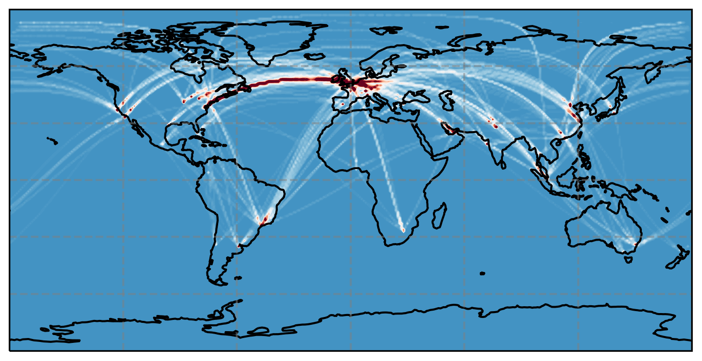
Figure 1 World map of H₂O emission locations (white to red) by LAPCAT aircraft, summed over all vertical levels. A color bar is not included, because the motivation is to depict specifically the emission location. Only one plot representative for all HIKARI emission scenarios is shown, because hypersonic features of emission are dominant in the vertical sum, and ZEHST and LAPCAT scenarios show quite a similar horizontal distribution on the world map. A vertical distribution is shown in Fig. 2.

While we focus on H₂-driven aircraft in this study, the HIKARI emission inventory includes carbon-based emission data as well. In general, H₂-driven aircraft with air-breathing engines emit H₂O and NO_x but potentially include unburned H₂ fuel. For the HIKARI emission inventory, 10 % of unburned H₂ is assumed.

In total, the HIKARI emission inventory contains three scenarios. In addition to the subsonic reference scenario based on an Airbus A350, a mixed-fleet scenario with ZEHST-type hypersonic aircraft and a mixed-fleet scenario with LAPCAT-type hypersonic aircraft are part of this inventory (Fig. 2). The respective cruise altitudes are approximately 12, 26, and 35 km. All aircraft designs travel from and to the same city pairs. The horizontal resolution is 1^∘ × 1^∘, and the vertical resolution is 304.8 m.

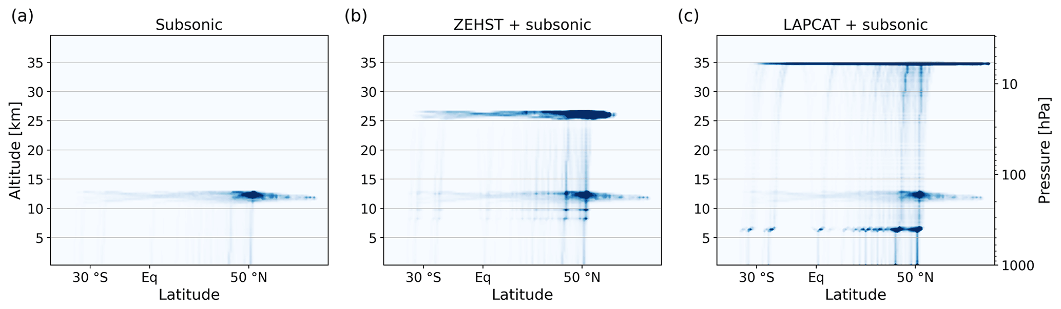
Figure 2 Zonal sum of trace gas emission location; (a) depicts the subsonic reference scenario, (b) depicts the ZEHST scenario, with a hypersonic market penetration of 9.8 %, and (c) depicts the LAPCAT scenario, with a hypersonic market penetration of 26.0 %. A color bar with units is not shown, since the location (altitude, latitude) is the interesting piece of information here. For annual amounts of emissions, see Table 2. The data is taken from the HIKARI project's emission inventory.

The collection of annual emissions of trace gases for the three scenarios are listed in Table 2. This includes the global emissions as well as the proportion emitted at stratospheric altitudes; the latter mostly consists of trace gases emitted at the cruise phase of hypersonic aircraft. For both the ZEHST and LAPCAT scenarios, approximately two-thirds of H₂O are emitted at stratospheric altitudes and one-third in the troposphere. The main part of NO_x is emitted at tropospheric altitudes, and H₂ is emitted to 76 % and more at stratospheric altitudes. Another property shown in the same table, market penetration, is a measure of how many of the global flight routes are suited for the specific hypersonic aircraft compared to subsonic aircraft. Hence, there is a smaller market for the aircraft LAPCAT, whose design is able to travel extremely large distances (approximately 18 000 km) due to the limited selection of appropriate city pairs like Brussels–Sydney. In comparison, ZEHST is a potentially faster alternative for 25 % of the subsonic aviation market with a smaller range (approximately 9 000 km). The aircraft designs differ in terms of passenger seats, with 60 for ZEHST and 300 for LAPCAT. In Fig. 2b and c, emission features at altitudes 6–11 km are visible. This originates from acceleration and climb to cruise altitude by the hypersonic aircraft of ZEHST and LAPCAT.

Table 2 HIKARI emission inventory. Annual emission of trace gas species H₂O, NO_x, and H₂. The upper three rows contain amounts of trace gases emitted in the whole atmosphere, while the lower three rows contain amounts of trace gases emitted at stratospheric altitudes only (above 100 hPa). Note that for ZEHST and LAPCAT, a part of the subsonic aviation is replaced by hypersonic transport; hence, the numbers depict whole air traffic scenarios.

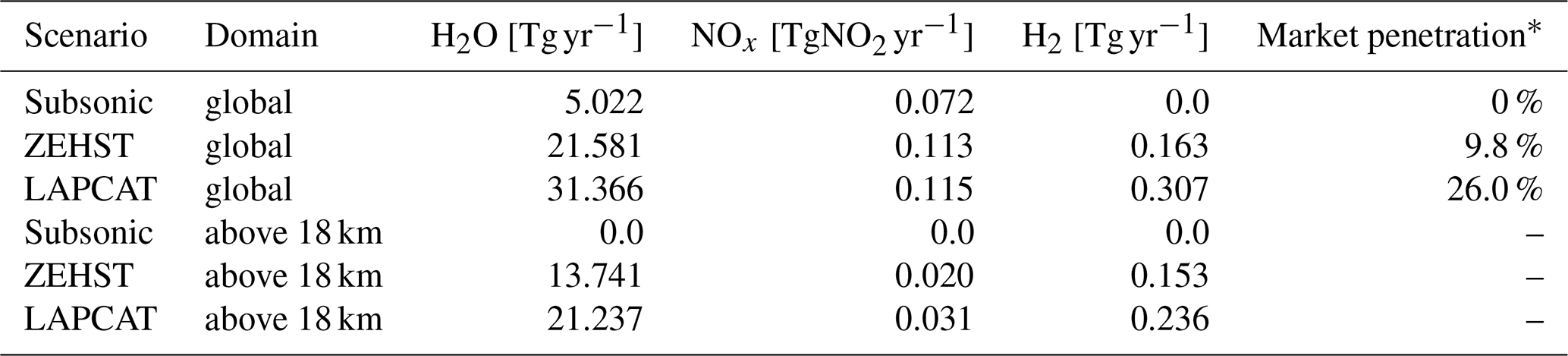
^* Market penetration depicts the ratio of subsonic-to-hypersonic aviation market, where hypersonic aircraft take over some of the subsonic market.

3.2 Spin up and temporal evolution

The respective full aircraft fleet is in operation for the total simulated time of 15 years. Annual emissions accumulate over the years, and perturbation of emitted trace gas concentration eventually reaches equilibrium at the multi-annual mean after 8–10 years. The emissions are balanced by transport and by loss to tropospheric altitudes as well as (photo-)chemical losses and production. Five years of simulation in equilibrium remain for average values and significance tests. The monthly mean mass perturbation above the tropopause (WMO, 1957) is shown in Fig. 3 over the simulation timeline from 2000 to 2015. EMAC and LMDZ-INCA show similar patterns of monthly oscillations. The oscillations of the latter are smoother, which is potentially related to the lower vertical resolution or the feedback between atmospheric composition and radiation in EMAC.

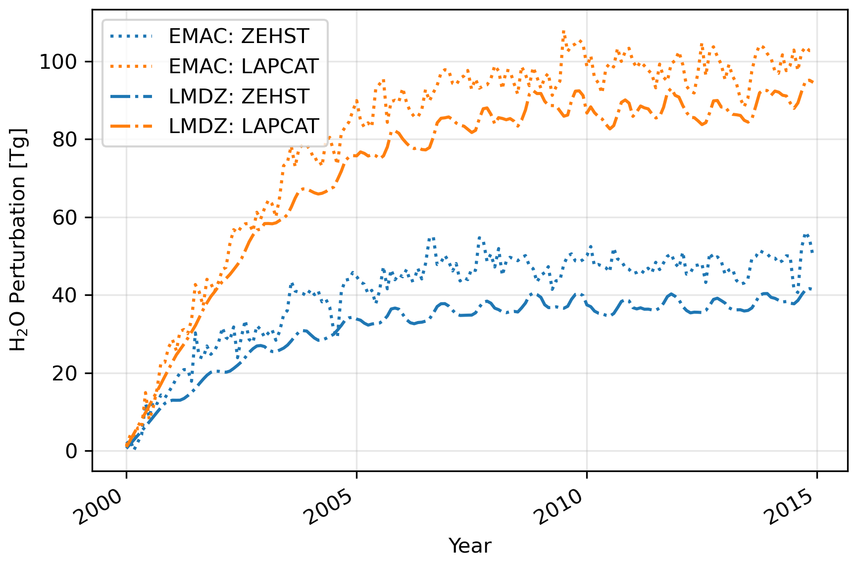
Figure 3 Temporal evolution of mass perturbation of H₂O in Tg above the tropopause. Blue and orange lines represent the ZEHST and LAPCAT scenarios, respectively. The annual amount of emitted trace gases is listed in Table 2.

After 15 years of the continuous operation of hypersonic fleets, the total emission of trace gases for ZEHST and LAPCAT scenarios at stratospheric altitudes are 206 and 319 Tg of H₂O, 0.3 Tg and 0.5 TgNO₂ of NO_x, and 2.3 and 3.5 Tg of H₂, respectively. During the 15 years, the emitted trace gases, while being chemically converted, are continuously transported to tropospheric altitudes, and only parts of the total emitted trace gases remain as perturbation. More information on the equilibrium perturbation is presented in Sect. 5.

4 Model evaluation

In this chapter, we evaluate the model results with observations from commercial aircraft. It is important to verify the model's performance in the upper troposphere–lower stratosphere region, especially in the northern extratropics, where most of the trace gases are emitted and the downward stratosphere-to-troposphere transport (SST) occurs. The SST, including the trace gases emitted at stratospheric altitudes, is a very important step in the continuous process that eventually removes these trace gases from the atmosphere – a fact that is further emphasized by the results of this publication. IAGOS offers data particularly fit for this region of interest. In a forthcoming publication, we extend the evaluation to higher altitudes and compare EMAC model results to satellite data (Pletzer and Grewe, 2022). In addition, a comparison between LMDZ-INCA and ozone sounding measurements has also been presented in Terrenoire et al. (2022).

4.1 Observation dataset

The research infrastructure IAGOS provides in situ measurements onboard a fleet of commercial aircraft. Observations of ozone and water vapor started in August 1994 and are still being collected to date. IAGOS mostly samples the UTLS in the northern extratropics, with cruise data spreading between 9 and 12 km above sea level. The ozone instruments are based on UV-absorption spectrometry, and their accuracy, precision, and time response are 2 ppb, 2 %, and 4 s, respectively. H₂O is measured using a capacitive hygrometer. The latter's precision and time response are generally 5 % – or 6 % in the thermal tropopause at midlatitudes (Smit et al., 2014) – for relative humidity and 5–300 s for H₂O, respectively, with regard to ice (Helten et al., 1998; Neis et al., 2015).

In order to allow a direct comparison between simulation outputs and the IAGOS data, the Interpol-IAGOS software (Cohen et al., 2021a) used here first projects observations onto model grids and then derives monthly means. The subsequent products are called IAGOS-DM-INCA and IAGOS-DM-EMAC. The -DM suffix refers to the distribution onto the model grid. Since the outputs from the models have a daily resolution, a mask is applied with respect to the IAGOS sampling. The subsequent products are called INCA-M and EMAC-M. The -M suffix refers to the mask. In this way, the monthly means derived from both the IAGOS and the simulations datasets represent the same days for each grid cell.

Seasonal and annual climatologies are then calculated on the 3D model grids. As in Cohen et al. (2021a), a grid point is filtered out if the total amount of IAGOS data are below a minimum threshold, the latter decreasing with latitude in order to account for the grid cell area. The validated grid points are then averaged together as partial columns, with a 400 hPa lower bound in order to exclude the IAGOS data recorded during ascent and descent phases near airports. In order to ensure a correct vertical representation, we select only the columns derived from at least two grid cells. Our assessment focuses on the northern midlatitudes, since, firstly, the UTLS is far more influenced by the stratosphere in the extratropics than in the tropics, and, secondly, only the UT is sampled in the tropics. The seasons defined in the northern midlatitudes are thus typically extratropical.

The scores used for the evaluation are the modified normalized mean bias (MNMB) and the Pearson correlation coefficient. For a set of N grid cells with an observed value o_i and a simulated value m_i, the MNMB is defined as follows:

$$\begin{array}{}\text{(1)}& \mathrm{MNMB}={\displaystyle \frac{\mathrm{2}}{N}}\sum _{i=\mathrm{1}}^N{\displaystyle \frac{m_i-o_i}{m_i+o_i}}.\end{array}$$

In contrast to the classical mean bias, which is sensitive to larger values, the MNMB treats large and small values with a similar sensitivity. Thus, it is very valuable for an assessment in the UTLS without separating tropospheric and stratospheric air masses. Indeed, since the tropopause altitude varies geographically, the aircraft fleet will record an important geographical variability in both ozone and water vapor.

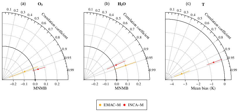
Figure 4 Taylor diagrams showing the assessment of the simulations against IAGOS in the northern extratropical UTLS. From (a) to (c), ozone, water vapor, and temperature are represented. For ozone and water vapor, the radial axis shows the modified normalized mean bias and the mean bias for the temperature. The error bars represent the interquartile interval. The orthoradial axis displays the Pearson correlation coefficient.

4.2 Model comparison to IAGOS observations

The evaluation of the simulations from EMAC and LMDZ-INCA against IAGOS in the northern extratropics are synthesized in the Taylor diagrams shown in Fig. 4 and in Figs. A6 and A7 in the Appendix for the seasonal scale. They are derived from the mean climatologies shown in Figs. A8–A12. Both model products are well correlated with the observations, with r∼0.90 for water vapor in INCA-M and r∼0.95 in the other cases. Independent of the magnitude, the models capture the geographical variations well for ozone, water vapor, and temperature. On annual average, the INCA-M product is characterized by a relatively weak mean bias in ozone, water vapor, and temperature. The EMAC-M product has a systematic cold bias in the extra-tropics, with half of the grid cells ranging between −3.8 and −2.5 K. It leads to an upward shift of the tropopause and thereby underestimates ozone and overestimates water vapor volume mixing ratios. These two features are visible in Fig. A8, where it is shown to be more representative of the higher latitudes. Lastly, according to Figs. A6 and A7, the ozone and water vapor biases keep the same sign through the seasons for EMAC-M, contrary to INCA-M. The ozone (respectively, water vapor) MNMB are particularly negative (respectively, positive) in both models during summer, possibly suggesting an increased underestimation of the stratospheric influence on the UTLS during this season.

5 Atmospheric composition changes

5.1 Water vapor

Stratospheric water vapor (SWV) stems mostly from upward transport at tropical latitudes and from oxidation of CH₄. The main factors for the loss of SWV are the reaction with O(¹D), photolysis, and the transport into the troposphere at the subtropical tropopause breaks. Additionally, polar stratospheric clouds cause dehydration through sedimentation of particles. Note that these processes are considered in our model simulations. Figure 5 shows the volume mixing ratio in equilibrium for the respective model and aircraft as a 5-year average (2010–2014). The SWV perturbation is clearly visible in both models, especially at the northern hemisphere, with the maximum located at around 50–60^∘ N, which overlaps with the maximum trace-gas emission location. Overall, the perturbation patterns agree well between the models, especially for altitudes from 16 to 37 km (approximately 100–4 hPa) and with differences at higher altitudes of 37 to 79 km (approximately 4–0.01 hPa). The latter altitude range contains only a small amount of the mass perturbation in the models, since the largest mass perturbation accumulates in the middle and lower stratospheres, where air density is larger (Figs. A2, A3). A t test shows that all zonal mean H₂O perturbations are statistically significant at a 99.9 % level and that only parts in the tropical UTLS (EMAC: ZEHST, LMDZ-INCA: ZEHST, LAPCAT) do not reach that value.

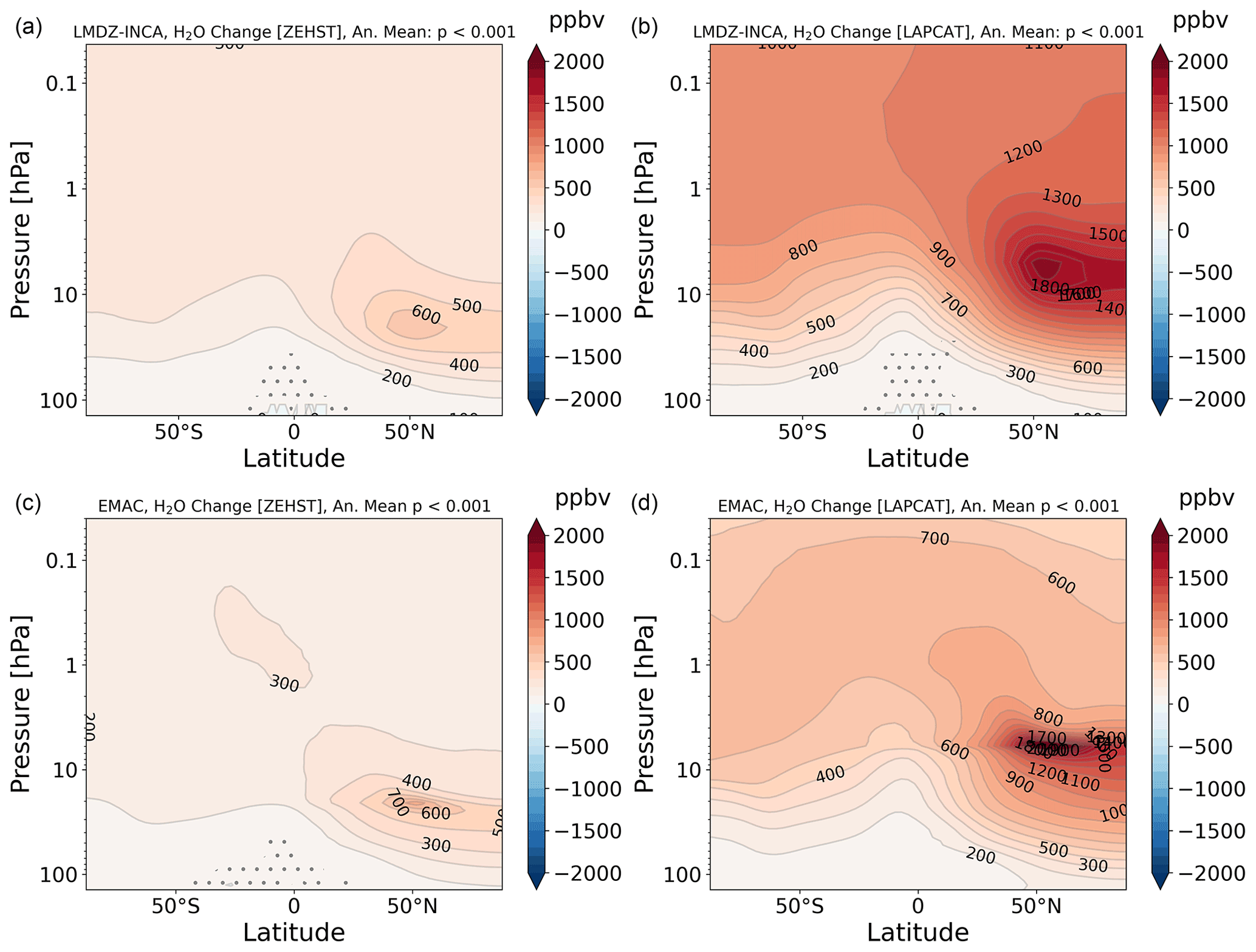
Figure 5 Multi-annual mean (2010–2014) of H₂O perturbations (ppbv) for the ZEHST scenario (a, c) and the LAPCAT scenario (b, d) for both models LMDZ-INCA (a, b) and EMAC (c, d) after approximately 13 years of continuous emission. Cruise altitudes are approximately at the respective perturbation maxima. The dotted region corresponds to the grid points where the mean perturbations are not significant at a 99.9 % level.

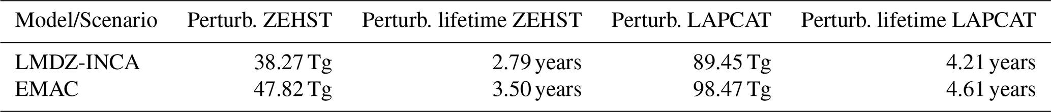
Absolute values of the mass perturbation and the respective perturbation lifetime of water vapor are listed in Table 3. Values were calculated for the perturbation above the tropopause (WMO, 1957). The total H₂O mass perturbation for each model is approximately twice as large for the higher flying aircraft compared to the lower flying aircraft due to the longer transport to the troposphere and due to the larger emission. The perturbation lifetime clearly increases with cruise altitude from 2.8–3.5 to 4.2–4.6 years. Due to the difference in annual H₂O emissions of both aircraft, the perturbation lifetime scales differently compared to the mass perturbation.

Table 3 Perturbation and perturbation lifetime of H₂O in teragram and years, respectively, for the ZEHST and the LAPCAT scenario and for each of the two models.

Mass perturbation and perturbation lifetime are affected by the (photo-)chemical removal of emitted water vapor. The key processes are photolysis and reaction with O(¹D). The combined average lifetime is shown in Fig. 6 for LMDZ-INCA (panel a) and EMAC (panel b). Photolysis clearly increases with altitude, resulting in the shortest lifetime at the upper end of the simulated altitude range and at the Equator region, where incident sunlight is strongest on average. The reaction with O(¹D) has a maximum at around 45–50 km, where the loss of O₃ due to photolysis and thus concentrations of excited atomic oxygen O(¹D) are generally larger. The combination mainly shows the features of H₂O+O(¹D), with contributions of photolysis at altitudes above 50 km.

Figure 6 Zonal mean (photo-)chemical H₂O lifetime in days dependent on photolysis and reaction with O(¹D) for LMDZ-INCA (a) and EMAC (b). Figure A5, showing both reactions independently, can be found in the Appendix.

Clearly, the (photo-)chemical destruction increases with altitude. However, our results show that the perturbation does not decrease with altitude. To verify the chemical loss and production of water vapor, we introduced an additional diagnosis within EMAC. It is a budget calculation for all chemical loss and production terms with respect to water vapor. Further information on our setup can be found in the supplementary files meccanism.pdf and scavinism.pdf and the general explanation in the supplement of Sander et al. (2005). We find that 29 % and 60 % of the annual emitted water vapor (Table 2) is destroyed for ZEHST and LAPCAT, respectively, which is generally in agreement with Fig. 6, which indicates larger (photo-)chemical H₂O losses at higher altitudes. The absolute values of H₂O loss are shown as dark blue bars in Fig. 7.

$$\begin{array}{}\text{(R1)}& {\displaystyle }{\mathrm{H}}_{\mathrm{2}}\mathrm{O}+hv\to \mathrm{H}+\mathrm{OH}\text{(R2)}& {\displaystyle }{\mathrm{H}}_{\mathrm{2}}\mathrm{O}+\mathrm{O}{(}^{\mathrm{1}}\mathrm{D})\to \mathrm{2}\mathrm{OH}\text{(R3)}& {\displaystyle }{\mathrm{HO}}_{\mathrm{2}}+\mathrm{OH}\to {\mathrm{H}}_{\mathrm{2}}\mathrm{O}+{\mathrm{O}}_{\mathrm{2}}\end{array}$$

The main drivers are photolysis and the reaction with O(¹D) (Reactions R1 and R2, Fig. 7 upper blue bars), where the reaction with O(¹D) dominates for both aircraft scenarios. The other reactants responsible for H₂O destruction – N₂O₅, ClNO₃, and BrNO₃ – do not contribute significantly.

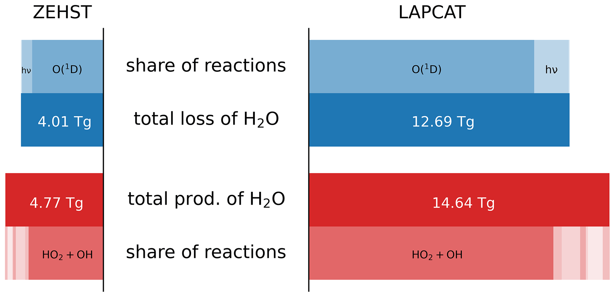
Figure 7 Bar plot of annual chemical loss and production perturbation of H₂O at stratospheric altitudes (100–0.1 hPa) for the ZEHST (left) and the LAPCAT (right) scenarios due to emitted trace gases (scenario–reference). This diagnosis includes a total of five H₂O-destroying and 45 H₂O-producing chemical reactions. The most relevant reactions of loss and production are shown as bright red and blue bars. Additionally, all dominant reactions of production are presented in detail in Fig. 8.

However, there is not only loss but also production of water vapor, which even overcompensates for the loss by 0.76 and 1.95 Tg in the cases of ZEHST and LAPCAT, respectively (dark red bars). This equals an increase in the initial annual perturbation above 18 km by 5.53 % for the former and 9.32 % for the latter. The resulting change from emissions and (photo-)chemistry is balanced by transport to the troposphere. The most important reaction for water vapor production is Reaction (R3), which, on the one hand, destroys hydroxyl and hydroperoxyl, and on the other hand, produces water vapor.

$$\begin{array}{}\text{(R4)}& {\displaystyle }{\mathrm{CH}}_{\mathrm{4}}+\mathrm{OH}\to {\mathrm{H}}_{\mathrm{2}}\mathrm{O}+{\mathrm{CH}}_{\mathrm{3}}{\mathrm{O}}_{\mathrm{2}}\text{(R5)}& {\displaystyle }\mathrm{HCHO}+\mathrm{OH}\to \mathrm{CO}+{\mathrm{H}}_{\mathrm{2}}\mathrm{O}+{\mathrm{HO}}_{\mathrm{2}}\text{(R6)}& {\displaystyle }{\mathrm{HNO}}_{\mathrm{3}}+\mathrm{OH}\to {\mathrm{H}}_{\mathrm{2}}\mathrm{O}+{\mathrm{NO}}_{\mathrm{3}}\text{(R7)}& {\displaystyle }{\mathrm{HNO}}_{\mathrm{4}}+\mathrm{OH}\to {\mathrm{H}}_{\mathrm{2}}\mathrm{O}+{\mathrm{NO}}_{\mathrm{2}}\end{array}$$

We call the surplus of production over destruction net-recombination. This net-recombination originates from different sources, and the significant reactions for production are shown in Fig. 8. Absolute values of production – 4.77 and 14.6 Tg yr⁻¹ for ZEHST and LAPCAT, originally from Fig. 7 – are shown here with additional information. In total, 45 reactions contribute to H₂O production; we grouped the reactions into four different categories, which are reactions with C–, N–, Cl–, and H–O compounds. The main contributors by far are the HO_x cycle (green) followed by either the more efficient methane oxidation for LAPCAT (red) or the contributions of nitric acids HNO₃ and HNO₄ for ZEHST (blue). The ratio of the categories is different for the two altitudes. H–O compounds contribute more to emission at the higher altitude.

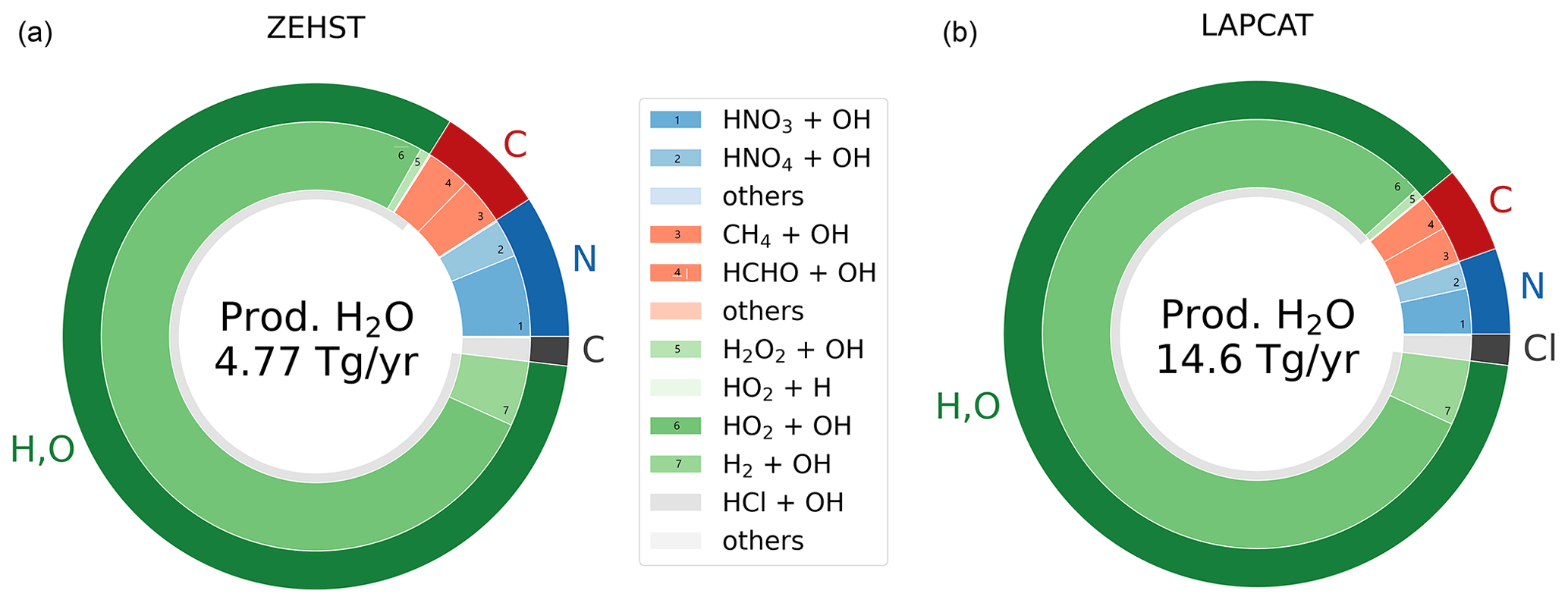
Figure 8 Pie plots on chemical reactions responsible for H₂O production derived from the EMAC simulation results (scenario–reference). (a) ZEHST scenario. (b) LAPCAT scenario. The darker outer ring shows the molecular category the reactions belong to (carbon-, nitrogen-, chlorine-, or hydrogen-based). The total sum of H₂O production is written in the center. The colored inner ring shows the proportion of different reactions within each category. We added black numbers in the legend and in the bright inner ring to represent the relation in addition to colors.

The photochemical depletion of H₂O and the shift to H₂ concentrations (e.g., Fig. 5.23, p. 312, Brasseur and Solomon, 2005) clearly does not limit the water vapor perturbation lifetime at these emission altitudes. So in contrast to the expected removal of emitted H₂O by photochemical depletion, we found a previously unknown importance of water vapor recombination for hypersonic emissions. Several reactions, including the hydroxyl radical, actually overcompensate for the photochemical depletion of H₂O perturbations. The overcompensation results in a net-recombination (recombination–depletion > 0) that is driven by HO_x recombination (mainly Reaction R3) as well as increased methane (Reactions R4 and R5) and nitric acid oxidation (Reactions R6 and R7). Both models show an increase in H₂O perturbation lifetime and H₂O perturbation at higher altitudes, which is further increased by the net-recombination. Our finding is robust, with good agreement between the two models.

5.2 Nitrogen oxides NO_x and ozone O₃

Continuous emission of NO_x (NO+NO₂) by hypersonic aircraft has a significant impact on ozone chemistry. The family of perturbed NO compounds is collectively described as NO_y (NO_x + and their nitrogen reservoir species). While NO_x is very reactive in catalytic cycles of ozone chemistry, NO_y additionally includes more stable molecules, like nitric acid (HNO₃), that act as a sink and remove NO compounds from catalytic ozone cycles for a longer time compared to NO_x. Figure A4 shows the perturbation of NO_x for each model and each aircraft fleet. In general, the perturbation patterns are similar, but EMAC results show a more detailed perturbation pattern. For LMDZ-INCA, we see a general NO_x increase, whereas in EMAC, additionally, we see that a decrease is visible at approximately 1 hPa upwards, ranging from equatorial regions to midlatitude regions for LAPCAT. In comparison, LMDZ-INCA shows one cluster of NO_x perturbation originating from the emission location (purple bar), while EMAC shows several (some not significant) clusters. The cluster locations seem to overlap, but the larger emission of LAPCAT makes it difficult to distinguish the clusters, as it covers the clusters interspace. The clusters appear at two levels, i.e., at cruise altitudes and at higher altitudes, just below 1 hPa. Results for the lower flying aircraft are more often outside of the 5 % uncertainty margin in comparison to the higher flying aircraft. This may be related to the larger emission of the latter, resulting in a larger perturbation, which differs from zero perturbation with higher confidence.

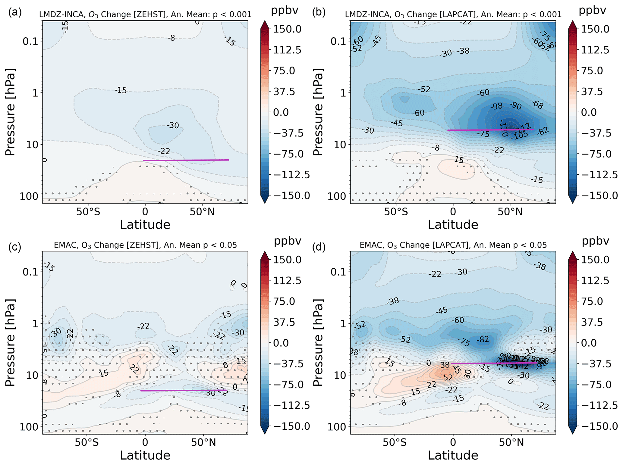
Figure 9 Multi-annual mean (2010–2014) of ozone perturbation (ppbv) for the ZEHST scenario (a, c) and the LAPCAT scenario (b, d) for both models LMDZ-INCA (a, b) and EMAC (c, d). Purple lines represent respective cruise altitudes. Hatched areas are characterized by a p value higher than the threshold indicated in the title of each plot.

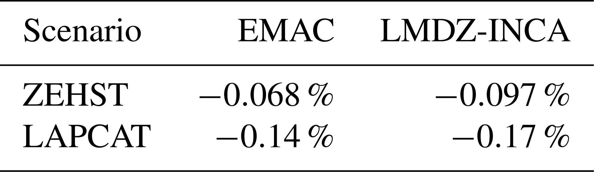
As mentioned before, NO_x are very reactive in catalytic cycles of ozone chemistry. The perturbation of ozone mainly resulting from H₂O and NO₂ emissions is shown in Fig. 9. The correlation between the increase of NO_x and the decrease of O₃ is clearly visible in the patterns at mid-stratospheric altitudes and especially at the cruise altitudes. LMDZ-INCA shows a slight increase originating from the tropical UTLS and a decrease with multiple clusters everywhere else, apart from no perturbation at lower latitudes at the highest altitude. EMAC results show a higher vertical resolution pattern, with clusters of O₃ increasing and decreasing, which may be due to the higher vertical resolution of EMAC (90 vertical grid levels) compared to LMDZ-INCA (39 vertical grid levels) in this study. The O₃ increase in areas below an O₃ decrease has already been reported by Solomon et al. (1985), and they expect a larger effect for lower latitudes, which would agree with our results. Worthy of note is that the area of O₃ increase overlaps with the area where NO_x perturbations are close to zero. Additionally, more of the high-energy radiation should reach lower altitudes due to the decrease above the area of O₃ increase. To conclude, the uncertainties due to the annual variability are lower in LMDZ-INCA compared to EMAC for both O₃ and NO_x, highlighting the significance of LMDZ-INCA results. The larger vertical resolution in EMAC could explain the different uncertainty value (p<0.05 for EMAC, p<0.001 for LMDZ-INCA), since it allows more detailed perturbation patterns, which is not model-specific but rather resolution-specific. If this is the case, this originates from the difference in vertical resolutions and not from the models themselves. The total reduction of O₃ is listed in Table 4. In general, results are of the same order of magnitude. Both models show the same trend that the higher flying aircraft fleet has a larger impact on O₃, and for both aircraft, the perturbation is slightly larger in LMDZ-INCA results.

Table 4 Relative total ozone mass change for each model and each aircraft fleet.

6 Radiation and climate

The radiative forcing (RF) caused by atmospheric composition changes depends very much on location (Lacis et al., 1990; Riese et al., 2012). In our results, the largest water vapor concentration change appears at lower stratospheric altitudes and increases poleward (Figs. A2, A3). The differences between the ZEHST and LAPCAT scenarios, except for magnitude, are small. Additionally, we described the ozone increase in the lower tropical stratosphere, where the RF sensitivity and air density are larger (concentration changes not shown). Hence, according to Lacis et al. (1990) and Riese et al. (2012), we expect a warming for both ozone and water vapor changes.

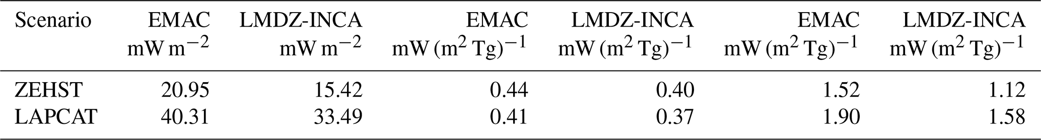
The annual radiative impact was calculated with the metric of stratosphere-adjusted radiative forcing at tropopause level using the equilibrium perturbation of H₂O, O₃, and CH₄. Atmospheric composition changes were used to calculate the RF with both models. The spin-up phase was three months, and the averaged result is based on 12 monthly means. The resulting RF for both models and both aircraft fleets are listed in Table 5, with the LAPCAT scenario showing larger values, which is mainly due to the larger water vapor perturbation. The normalized RF per teragram of water vapor perturbation is in good agreement with an average and standard deviation of 0.43±0.02 and 0.39±0.02 mW (m² Tg)⁻¹ for EMAC and LMDZ-INCA, respectively. Another measure, the RF per teragram of annual water vapor emission, shows that the normalized RF correlates with altitude; the values are 25 %–41 % larger for LAPCAT in both model results.

Table 5 Radiative forcing per year in mW m⁻² per teragram of H₂O perturbation and per teragram of annual water vapor emission (from Table 2), both in mW (m² Tg)⁻¹, for each scenario and model, calculated with atmospheric composition changes of H₂O, O₃, and CH₄.

The perturbations of H₂O, O₃, and CH₄ above the meteorological tropopause were used to calculate the RF (approximately 100 hPa at tropical and 300 hPa at polar latitudes). The direct impact of hydrogen perturbation on RF is not significant, and their indirect effect – i.e., on O₃ and H₂O mixing ratios – is included and will be reported in a separate publication in more detail (Pletzer and Grewe, 2022). In comparison, the contribution to RF of H₂O is largest, followed by O₃ and a negative RF due to CH₄ reduction. The negative RF of the latter is due to the enhanced methane oxidation and is larger for the LAPCAT scenario, where hydroxyl radicals are clearly more active (Fig. 7). The detailed values with short- and longwave contributions are listed in Table 6.

Table 6 Short- and longwave contributions (respectively, SW and LW) to radiative forcing (RF) in mW m⁻².

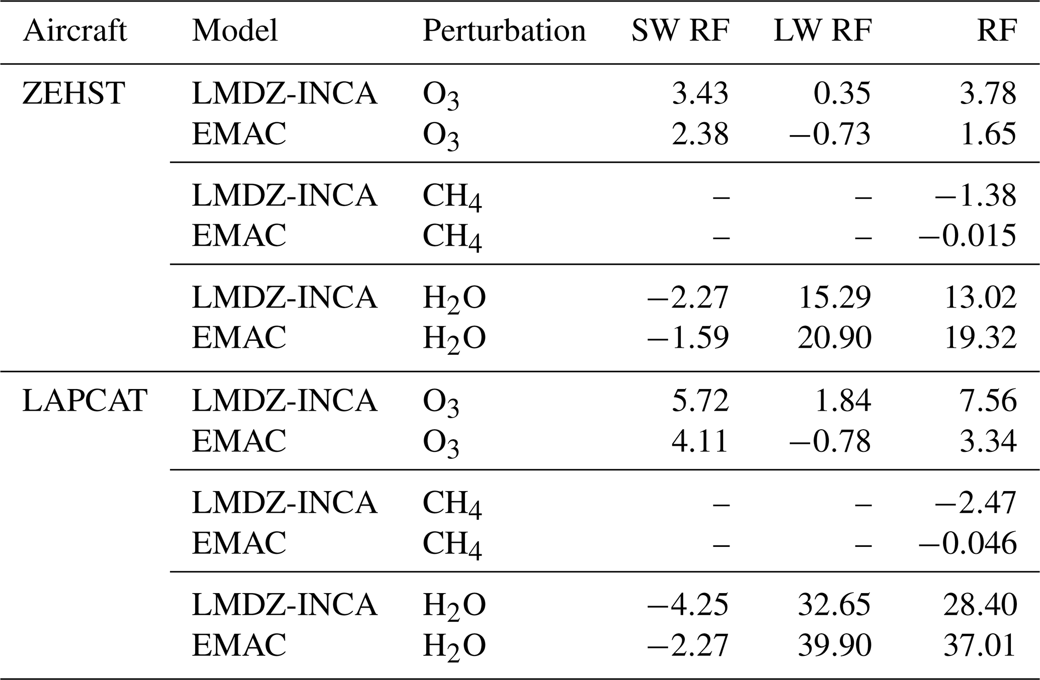
LMDZ-INCA shows a smaller longwave RF (LW RF) and a larger negative shortwave RF (SW RF) for H₂O compared to EMAC. Ozone longwave RF has a negative sign for EMAC and a positive sign for LMDZ-INCA. The differences in magnitude and sign of O₃ longwave RF may originate from the varying atmospheric composition changes in EMAC, with areas of ozone increase and decrease. This altitude dependency very much affects the contribution to RF, as has been shown by Lacis et al. (1990) and Hansen et al. (1997). An additional test shows that the ozone increase in the UTLS compensates for the negative longwave forcing due to the high sensitivity to ozone changes and explains the positive longwave value for LMDZ-INCA. Ozone shortwave RF is generally larger by 40 %–44 % for LMDZ-INCA compared to EMAC. Methane net RF is 1–2 orders of magnitude smaller for EMAC compared to LMDZ-INCA. A comparison of the change in global methane lifetimes is shown in the Appendix. There, methane lifetime change is larger for the LAPCAT compared to the ZEHST scenario for both models, and the methane lifetime is, in general, less by a factor of three and two for EMAC compared to LMDZ-INCA for both ZEHST and LAPCAT scenarios, respectively. To conclude, the reason for the different magnitude in methane net RF is not fully clear and should originate from the RF calculation. However, the contribution of methane to RF is small in both models compared to H₂O and O₃ and should not affect our results.

For the largest contributor to RF, the H₂O perturbation, we have performed a comparison to other radiation calculations. The performance test was done like in Myhre et al. (2009). That means we calculated the impact on RF by increasing the water vapor mixing ratio from 3.0 to 3.7 ppmv above the tropopause. The LMDZ-INCA result is 0.18 W m⁻², which is below the mean of Myhre et al. (2009) (mean 0.25 W m⁻², range 0.16–0.38 W m⁻²), while the EMAC result is larger than the mean, with 0.28 W m⁻². Both models are in the range of different models presented by Myhre et al. (2009), with LMDZ-INCA at the lower and EMAC in the mid-upper range.

Perturbations at tropospheric altitudes were neglected, mainly due to the large variability of water vapor, either with a reset to reference water vapor during the perturbation simulations (LMDZ-INCA) or due to exclusion in the RF calculations (EMAC). Hence, for EMAC, the H₂O perturbations at tropospheric altitudes are not zero and therefore will contribute to the RF calculations. However, the upper tropospheric water vapor perturbations have a very large variability, since the 5 % confidence intervals for the mean are ±106 % and ±33 % for the ZEHST and LAPCAT scenarios, respectively. In comparison, for H₂O perturbations above the tropopause, variability is significantly smaller, with ±3.1 % and ±1.8 % for the ZEHST and LAPCAT scenarios, respectively. Hence, water vapor perturbation in the upper troposphere could contribute significantly to RF, but the associated error due to the large variability is significantly larger. Nonetheless, we calculated the RF with EMAC, including the tropospheric perturbations for comparison (see Table A1 in the Appendix). We found that the RF increases by approximately 51 % to 63 % when the upper tropospheric perturbations are included.

7 Discussion

7.1 Limitations of the model simulations

7.1.1 Aerosol and water vapor from volcanic origin

In our model simulations, we assume an atmosphere without volcanic eruptions. However, volcanic eruptions could occur during the decades of operation of new aircraft. Volcanic emissions, like water vapor or sulfate aerosols, affect the atmospheric composition in the stratosphere, especially through heterogeneous chemistry, and these changes are strongly dependent on latitude and season. The changes of lower stratospheric water vapor changes due to volcanic eruptions are on the order of two years and affect ozone concentrations (Stenke and Grewe, 2005). Sulfate aerosols are known to increase temperatures in the tropics and could, in turn, enhance the Brewer–Dobson circulation, eventually reducing the climate impact of hypersonic transport slightly. Overall, the topic is very complex in itself, and how hypersonic emissions and volcanic emissions influence each other remains to be answered with robust and topic specific simulations.

7.1.2 Strengthening of the Brewer–Dobson circulation

In our model simulations, we use atmospheric composition projections for the years 2050–2064 combined with present day meteorology (2000–2014). Hence, projections of the dynamic component are not included in our simulations. The main reason is that reanalysis data from the future are simply not available for nudging. Using another method was not an option, since we rely on nudging to have the same meteorology in both models for a high signal-to-noise ratio. However, the changes of dynamic processes like the Brewer–Dobson circulation due to climate change are very likely to be significant, and we therefore discuss the topic briefly (Butchart et al., 2006; Shepherd and McLandress, 2011). The associated transport is the dominant factor of water vapor perturbation lifetime and therefore of the climate impact of hypersonic aircraft. An increase in the strength of the stratospheric and mesospheric circulation would most likely reduce the climate impact of hypersonic aircraft. Butchart et al. (2006) estimate the troposphere–stratosphere mean mass exchange rate to increase by 2 % per decade (with considerable differences between the models). That would result in an approximately 8 %–10 % stronger circulation from 2050–2064, and in turn – if the effect can really be directly translated to perturbation lifetime – the climate impact of hypersonic aircraft would be reduced by approximately the same percentage.

7.2 Atmospheric composition changes

Here, we focus on the comparison to the publication by Kinnison et al. (2020). Using the coupled chemistry–climate model WACCM (Whole Atmosphere Community Climate Model), they estimate the ozone, water vapor, NO_x, and HO_x perturbations by a fleet of hypersonic aircraft in independent scenarios where aircraft, powered with conventional fuel, fly at 30 and 40 km. Similar to our model setups, WACCM simulates atmospheric chemistry and dynamics. For more detailed information, please refer to their publication. Similar to our setup, they look at atmospheric conditions for the year 2050; however, the averaged annual results are based on one year, while ours represent the mean over five years. In turn, a larger deviation from the long-term mean could be expected for their results. The total annual emission in their setup amounts to 58.3 Tg of H₂O and 0.94 Tg of NO₂, which is approximately 3 to 4 times larger for the former and 30 to 47 times larger for the latter compared to the annual values of the HIKARI data.

In agreement with our result, the H₂O perturbation for the higher flying aircraft fleet is significantly larger, and the perturbation patterns agree very well with the maximum perturbation being at midlatitudes in the northern hemisphere and at the cruise altitude. In their case, the total emission per trace gas is the same for both altitudes, which is not the case in our study, since the emissions in HIKARI are based on two different aircraft designs. Total values of mass perturbation were not published for H₂O and thus cannot be compared with ours. We presented the (photo-)chemical lifetime in Fig. 6. Here, the agreement of latitudinal and altitude features with Kinnison et al. (2020, Fig. 3) is very good in general. There are differences in magnitude from 50 km upward, increasing with altitude, where photolysis is dominant. If this originates from WACCM covering more of the atmosphere compared to our models – and thus being more accurate at 50 km upwards – is an open question. However, the stratosphere is well represented in the models used here, which is most important for the topic of our study, and the equilibrium mass perturbation at mesospheric altitudes is insignificant in comparison to stratospheric altitudes.

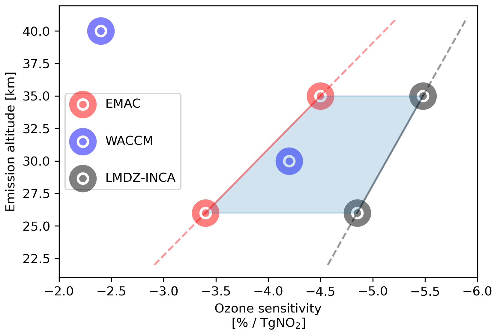
Figure 10 Ozone sensitivity, dependent on altitude of emission, from three different models WACCM, EMAC and LMDZ-INCA. Results from this work were calculated using values from Tables 2 and 4. Results for WACCM were published by Kinnison et al. (2020, Table 2). The shaded area highlights the good agreement of LMDZ-INCA and EMAC results with WACCM results for the region from approximately 26–35 km altitude.

7.2.1 Ozone sensitivity

The calculated ozone sensitivity with −4.2 % (Tg NO₂)⁻¹ and −2.4 % (Tg NO₂)⁻¹ for 30 and 40 km altitude (Kinnison et al., 2020, Table 2) is of the same order of magnitude compared to our results with −3.4 % (Tg NO₂)⁻¹ and −4.5 % (Tg NO₂)⁻¹ for EMAC and −4.9 % (Tg NO₂)⁻¹ and −5.5 % (Tg NO₂)⁻¹ for LMDZ-INCA at 26 and 35 km altitude, respectively. Figure 10 shows both results from our study and their study. Our results have a positive correlation between ozone sensitivity and altitude. This might point to a maximum of absolute ozone sensitivity at around 35 km altitude, since the absolute value for WACCM at 40 km altitude is already much smaller and since the models seem to agree very well for the region between 26 and 35  km. The assumed tropical maximum of the ozone mixing ratio of 31 km overlaps with this region and is very close to the maximum value. However, the altitude of emission often does differ from perturbation maxima of NO_x and O₃. Be aware that we are only presenting two data points per model, and to come to conclusions regarding the largest value of ozone sensitivity might be inaccurate. Additionally, there are some differences between the setups, e.g., Kinnison et al. (2020) estimate ozone sensitivity based on NO_x perturbations only and with a larger amount, while we look at the combined effects of NO_x, H₂O, and H₂ emission. Furthermore, the HIKARI data include a vertical distribution of emissions, in which take off and landing are present, and the fleet comprises not only hypersonic but subsonic aircraft as well, while they inject the emission in a single layer. The effect of tropospheric water vapor emission on SWV is negligible due to the tropical tropopause cold point, but NO_x emitted in the tropical troposphere may be transported to stratospheric altitudes and increase the uncertainty of the comparison. Note that, in another set of EMAC simulations from a forthcoming publication (Pletzer and Grewe, 2022) where NO_x is emitted in a single layer, we see an approximately equal ozone sensitivity at 30 and 38 km for tropical and midlatitudinal regions, while for northern polar regions the lower altitude has a sensitivity nearly twice as much as that of the higher altitude and shows a negative correlation very similar to Kinnison et al. (2020).

7.2.2 Contrail formation

Another type of atmospheric composition change that affects climate is the formation of contrails. A study from Stenke et al. (2008) estimates the change in contrail formation and the change of contrail radiative forcing for subsonic and supersonic aircraft by replacing parts of the subsonic fleet with supersonic aircraft. According to the authors, the change in contrail radiative forcing and the change in total contrail cover is very small. However, they report a shift of contrail cover from mid latitudes (200 hPa) to low latitudes (supersonic cruise altitude). For hypersonic aircraft, this relation might be changed. Hypersonic aircraft fly above the tropical tropopause, where temperatures are warmer, and hence do not form contrails in the tropics. Therefore, the replacement of subsonic with hypersonic aircraft would probably lead to a reduction of contrail radiative forcing.

7.3 Comparison to emissions at lower altitudes

Zhang et al. (2021, Fig. 11) published an altitude-dependent comparison of ozone and water vapor RF normalized to fuel use. To compare their results on climate impact, we used their emission index (EI(H₂O) = 1237 g (H₂O) kg fuel⁻¹) and fuel use (47.18 Tg) to recalculate their results to RF per emitted water vapor in teragram. With the above values, we extracted the linear relation of 0.1 mW m⁻²/2 km for an increase of RF with altitude. The extrapolation to ZEHST and LAPCAT cruise altitudes resulted in 0.93 and 1.56 mW m⁻² for ZEHST and LAPCAT, respectively. Compared to our results (1.1–1.5 and 1.6–1.9 mW m⁻² for ZEHST and LAPCAT, respectively), presented in Table 5, the values calculated here are generally lower than the EMAC results, especially compared to ZEHST. LMDZ-INCA results are lower for ZEHST compared to the extrapolation, though they agree astonishingly well for LAPCAT. Clearly, the linear relation is not a perfect fit; however, it shows the same trend, and the order of magnitude agrees very well.

7.4 Comparison to the climate impact of other aircraft designs

For a better comparison of hypersonic to sub- and supersonic aircraft, we included Fig. 11. It shows an enhancement factor, i.e., the ratio of the climate impact of a specific aircraft compared to a conventional subsonic aircraft, depending on altitude. The numbers shown there were calculated using the climate response model AirClim (Grewe and Stenke, 2008; Dahlmann et al., 2016). The subsonic estimate is based on contrail formation, CO₂, H₂O, and NO_x (short-lived ozone, primary mode ozone, methane) effects. The comparison is based on results from this study, Grewe et al. (2007, 2010), and Grewe (2021, available from ls@vki.ac.be or secretariat@vki.ac.be). While subsonic is the reference case with a value of 1, supersonic aircraft show a climate impact that increases with altitude. The hypersonic aircraft ZEHST follows that trend, with an enhancement factor of approximately 20 (near-surface temperature change or RF normalized to revenue passenger kilometers). However, the enhancement factor of the second hypersonic aircraft LAPCAT (PREPHA) is less than 10 due to its higher passenger capacity. Hence, a larger aircraft size, i.e., larger passenger number, is clearly a promising design option to reduce the climate impact per passenger and can compensate for the climate impact due to higher cruise altitudes. The error estimate (blue shaded area) includes the tropospheric region, with its very large variability (see Sect. 6). Blue squares represent an aircraft of type LAPCAT MR3, developed in the STRATOFLY project, for four different altitudes and based on a single trajectory (Viola et al., 2021a, b). There, the increasing climate impact with altitude is clearly visible.

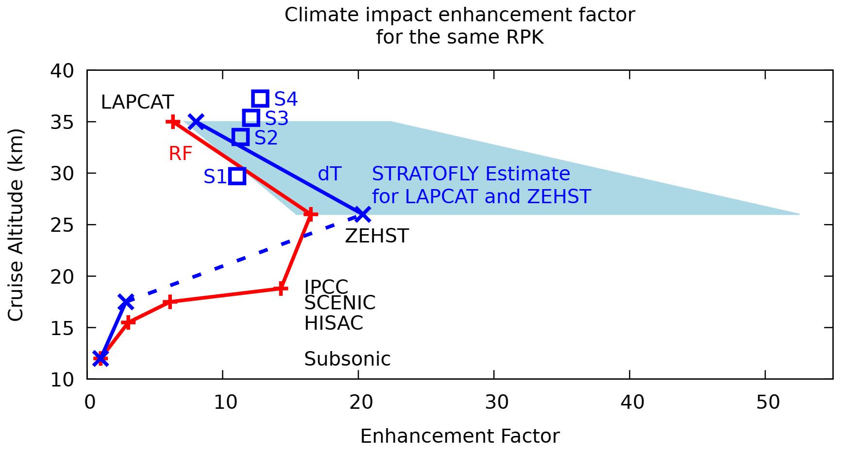
Figure 11 Radiative forcing (red) of a fleet of the respective aircraft 50 years after entry into service (EIS) and the near-surface temperature change (blue) based on the HIKARI project results. RPK (unit pax-km) refers to the revenue passenger kilometers, i.e., total kilometers traveled by all passengers on an aircraft or on a fleet of aircraft. The shaded area shows an uncertainty range from this work. This figure is taken from Grewe (2021) and includes the values of four STRATOFLY MR3 versions for different altitudes (S1 to S4) based on data published by Viola et al. (2021a, Table 2).

7.5 Climate impact of hypersonic aircraft

Estimates on the climate impact of hypersonic aircraft barely exist. A recent estimate was published by Ingenito (2018). He approximates the climate impact by a fleet of hypersonic aircraft (type LAPCAT II MR2.4, ESA, 2015) based on water vapor perturbation only. In his study, a fleet of 200 hypersonic aircraft fly from Brussels to Sydney 365 d a year and emit 376 Tg of water vapor, which results in a water vapor perturbation that increases surface temperature by 100 mK. We want to mention that the estimate is based on the correlation of an increase in global atmospheric water vapor and near-surface temperature from a third publication, and the whole calculation can be described as a 1D box model. For comparison to our results in Fig. 11, we normalize the change in surface temperature with passenger kilometers (pax-km). Therefore, we assume a distance of 16 367 km between Brussels and Sydney and a passenger capacity of 300 (LAPCAT II) and obtain a normalized near-surface temperature change of $\mathrm{396}\times {\mathrm{10}}^{-\mathrm{12}}$ mK (pax-km)⁻¹. This equals an enhancement factor of 61; hence, their estimate of the climate impact of hypersonic aircraft is 61, as much as subsonic aircraft. Compared to the enhancement factors in Fig. 11, this value is outside of the uncertainty range of our study. The upper limit of the uncertainty range is equal to RF calculations with composition changes, including upper tropospheric water vapor. These were neglected in the main calculations due to the large variability and the focus on stratospheric perturbation of trace gases.

We mentioned the significant contribution of upper tropospheric water vapor to RF in our model simulations with EMAC and want to elaborate some more, as this is important for comparison. In general, the lifetime of water vapor is comparably short at tropospheric altitudes (spreading from hours to approximately six months; Fig. 6a in Grewe and Stenke, 2008). However, in our study, the main emission is at midlatitudes, where water vapor lifetime is between 7 d and one month according to the reference. We did not test how well the tropospheric perturbation is represented in our model, since we focused on stratospheric perturbations in the EMAC setup. In EMAC simulations, the tropospheric water vapor was not reset nor nudged to ECMWF data in contrast to the LMDZ-INCA simulations. Therefore, the variability introduces a large error range in the upper tropospheric water vapor results compared to the results for the stratosphere in EMAC.

8 Summary

In this study, we calculated the radiative forcing and the climate impact of two different hypersonic aircraft designs, both fueled with liquid hydrogen. The difference in cruise altitude (26 and 35 km) results in significant differences in atmospheric perturbations, perturbation lifetime, and in turn, climate impact. Clearly, water vapor is the largest contributor to the latter. We find an efficient (photo-)chemical destruction of H₂O at higher altitudes, as expected based on theory (e.g., Fig. 5.23, p. 312, Brasseur and Solomon, 2005). However, we did not see a smaller H₂O perturbation at the higher emission altitude, which agrees with the tendency in the study by Kinnison et al. (2020). Our analysis shows, for the first time, that the recombination to H₂O overcompensates for the (photo-)chemical destruction of emitted H₂O, which results in a longer H₂O perturbation lifetime at the higher altitude (35 km). The overcompensation originates from an increased CH₄ and HNO₃ oxidation in addition to the HO_x recombination. This trend may change at even higher altitudes, where water vapor lifetime decreases and, more importantly, the lifetime of HO_x and H₂ increases substantially. Whether the recombination of emitted water vapor is affected has not been tested at these altitudes. The finding of longer H₂O perturbation lifetime and recombination contributes to the understanding of chemistry at stratospheric and lower mesospheric altitudes. For ozone, we report an overall depletion of the ozone layer, with a decrease at middle-to-upper stratospheric altitudes and an increase at lower stratospheric altitudes. This results in radiative warming for both aircraft, with a larger effect for the higher flying aircraft. The radiative impact of increased hydrogen is not significant compared to the other contributors and has a comparably small, indirect effect by contributing to atmospheric perturbations of CH₄, H₂O, and O₃. This will be addressed in more detail in a follow-up publication. The results can be deemed robust due to the usage of two high-end chemistry–climate models and the performance validation of radiative forcing due to stratospheric water vapor perturbation. To conclude briefly, the impact on climate of aircraft emitting water vapor and flying above the tropopause increases very much with altitude, since water vapor radiative forcing is significantly larger than ozone radiative forcing, which has a more complex altitude dependency. This is clearly shown by the increase of water vapor perturbation lifetime and normalized radiative forcing with altitude. Due to larger fuel consumption with higher speeds at high cruise altitudes on the one hand and the atmospheric conditions at these cruise altitudes (recombination, lifetime of H₂O) on the other, hypersonic aircraft have a considerable larger climate impact than subsonic and supersonic aircraft.

Appendix A

The applied EMAC model setup comprised the submodels AEROPT (AERosol OPTical properties), AIRSEA, CH4, CLOUD, CLOUDOPT (CLOUD OPTical properties), CONTRAIL, CONVECT (CONVECTion), CVTRANS (Convective Tracer TRANSport), DRADON (Decay RADioactive ONline), DDEP, E5VDIFF (ECHAM5 Vertical DIFFusion), GWAVE (Gravity WAVE), H2OEMIS, JVAL (J VALues), LNOX, MECCA, MSBM, O3ORIG (O3 ORIGin), OFFEMIS, ONEMIS, ORBIT, OROGW (OROgraphic Gravity Waves), PTRAC (Passive TRACers), QBO (Quasi Biannual Oscillation), RAD (RADiation), S4D (Sampling in 4 Dimensions), SATSIMS (Satellites Simulator), SCALC (Simple CALCulations), SCAV, SCOUT (Stationary Column OUTput), SEDI, SORBIT (Satellite ORBITs), SURFACE, TBUDGET, TENDENCY, TNUDGE (Tracer NUDG(E)ing), TREXP (Tracer Release EXperiments from Point sources), TROPOP (TROPOPause), and VISO (Vertically layered iso-surfaces and maps) (Jöckel et al., 2006, 2010; Roeckner et al., 2006). Further information is available on the MESSy homepage https://www.messy-interface.org/ (last access: 31 August 2022).

Table A1 Short- and longwave contributions to radiative forcing in mW m⁻² for EMAC, including upper tropospheric perturbation of water vapor, ozone, and methane, and the related error potential of approximately 51 % to 63 % due to the integration of tropospheric perturbations.

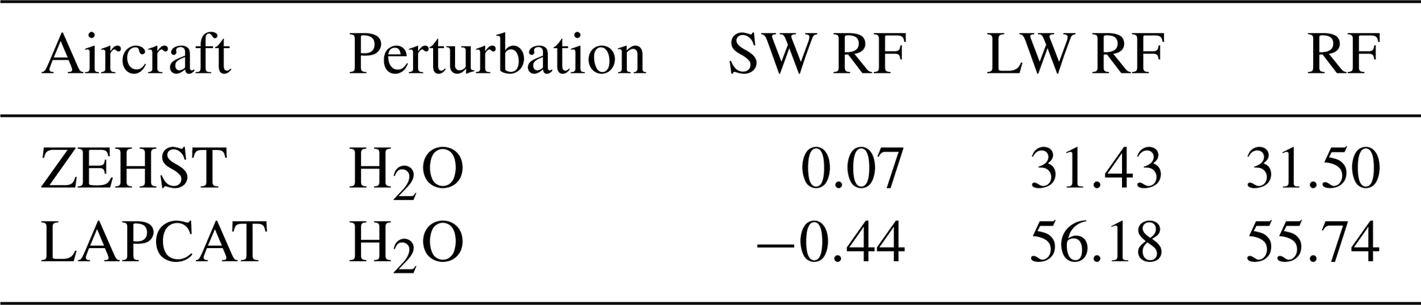
Table A2 Change in global methane lifetime for LMDZ-INCA and EMAC and the ZEHST and LAPCAT scenarios.

Figure A1 Vertical distribution of annual H₂O emission for ZEHST and LAPCAT. The peak at 6 km altitude comes from the hypersonic boost of the LAPCAT aircraft. The vertical distribution was aggregated for a better comparability (with a 2 km bin size). For the total amount of emissions, see Table 2.

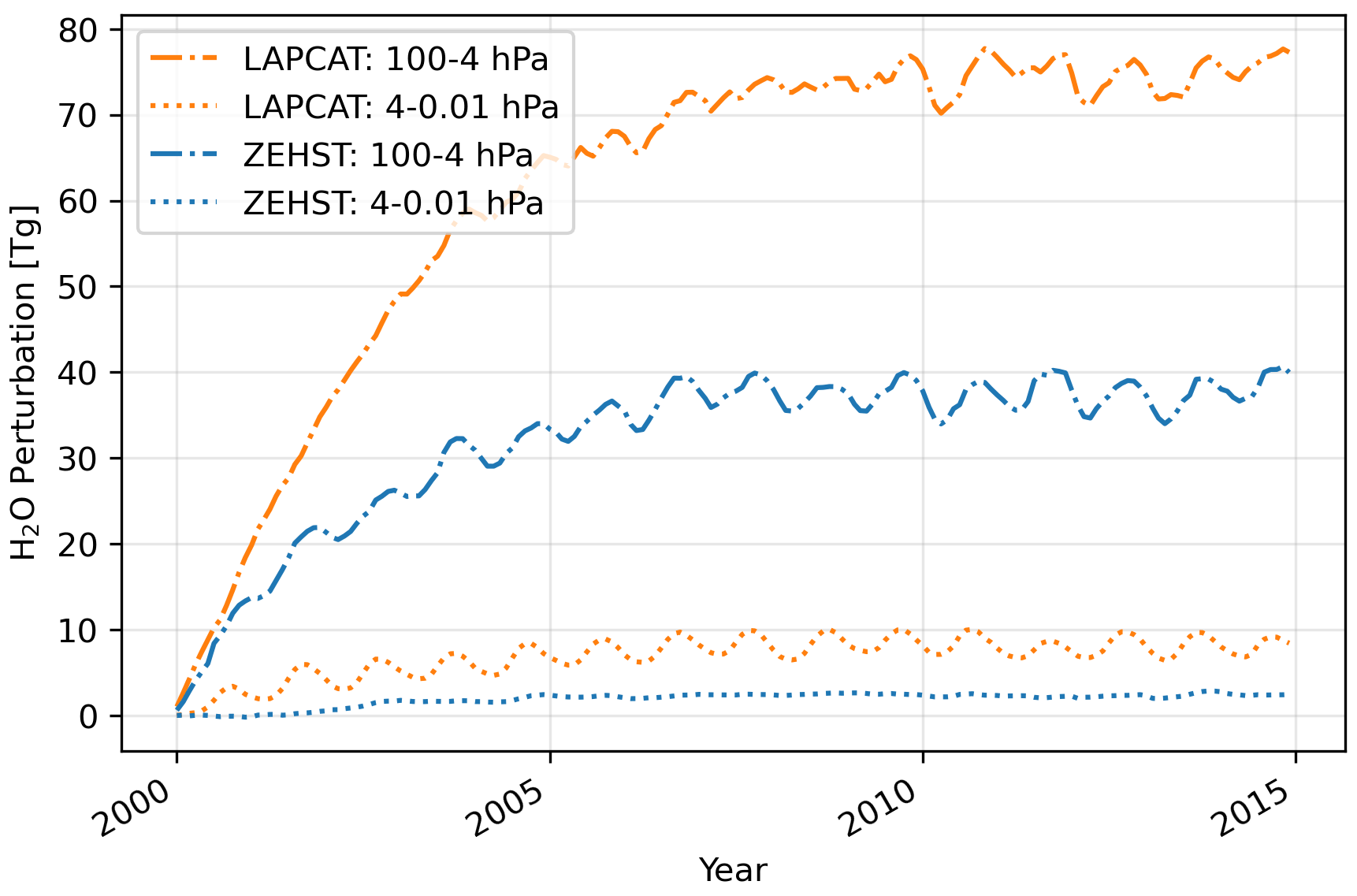
Figure A2 Timeline plot of accumulated trace gas H₂O in teragram, based on monthly mean values. Blue lines represent scenario ZEHST and orange lines represent scenario LAPCAT. Shown is the H₂O perturbation over time above 4 hPa (dotted) and from 4–100 hPa (solid-dotted).

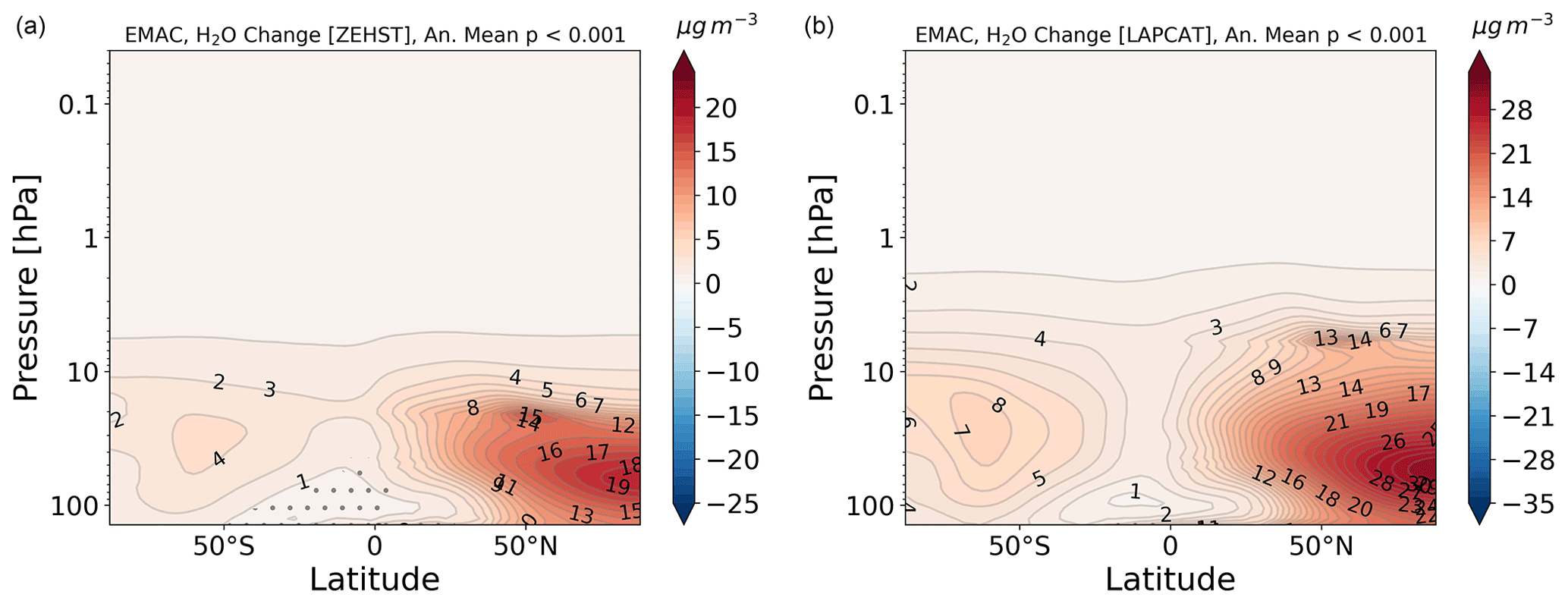
Figure A3 Multi-annual mean (2010–2014) of H₂O-perturbation [µg m⁻³] for the ZEHST scenario (a) and the LAPCAT scenario (b). Dotted areas represent probabilities larger than 0.1 % for data not to be significant (standard t test). Horizontal lines represent respective cruise altitudes.

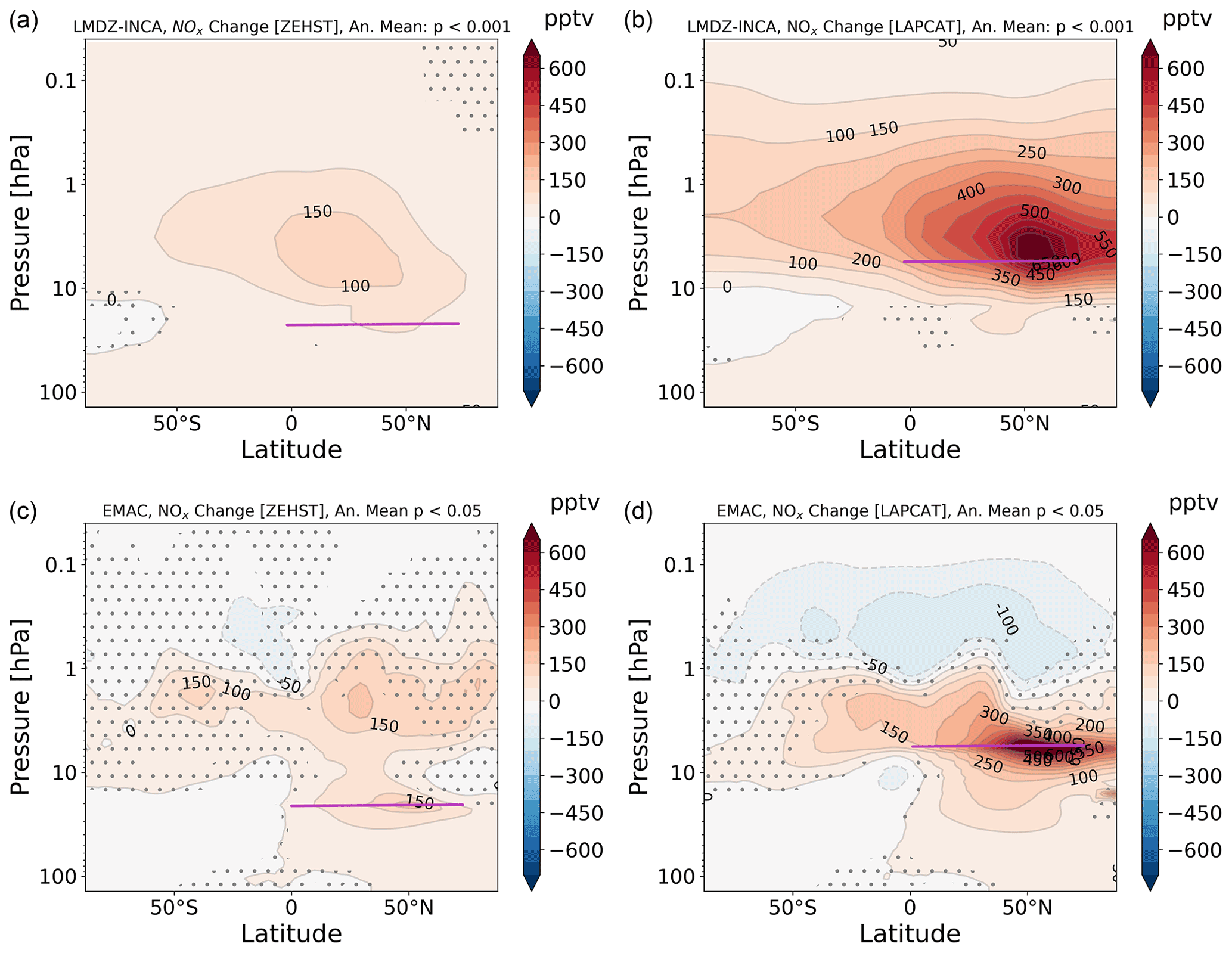
Figure A4 Annual mean (2010–2014) of NO_x perturbation (pptv) for the ZEHST scenario (a, c) and the LAPCAT scenario (b, d) for both models LMDZ-INCA (a, b) and EMAC (c, d). Purple lines represent respective cruise altitudes. Hatched areas are characterized by a p value higher than the threshold indicated in the title of each plot.

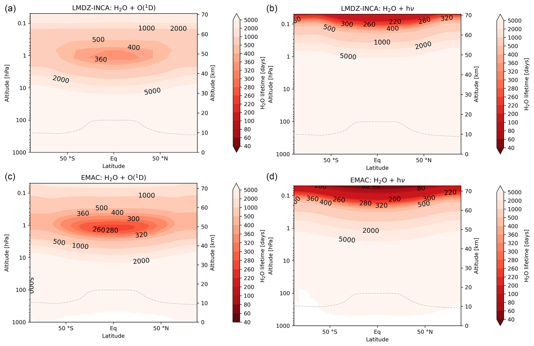
Figure A5 Zonal mean (photo-)chemical H₂O lifetime in days for photolysis (b, d) and reaction with O(¹D) (a, c) for LMDZ-INCA (a, b) and EMAC (c, d).

Figure A6 Same as Fig. 4 for winter (a–c) and spring (d–f).

Figure A7 Same as Fig. 4 for summer (a–c) and autumn (d–f).

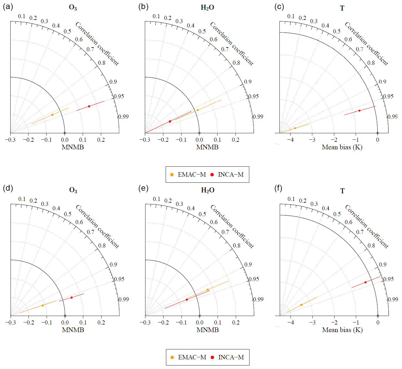
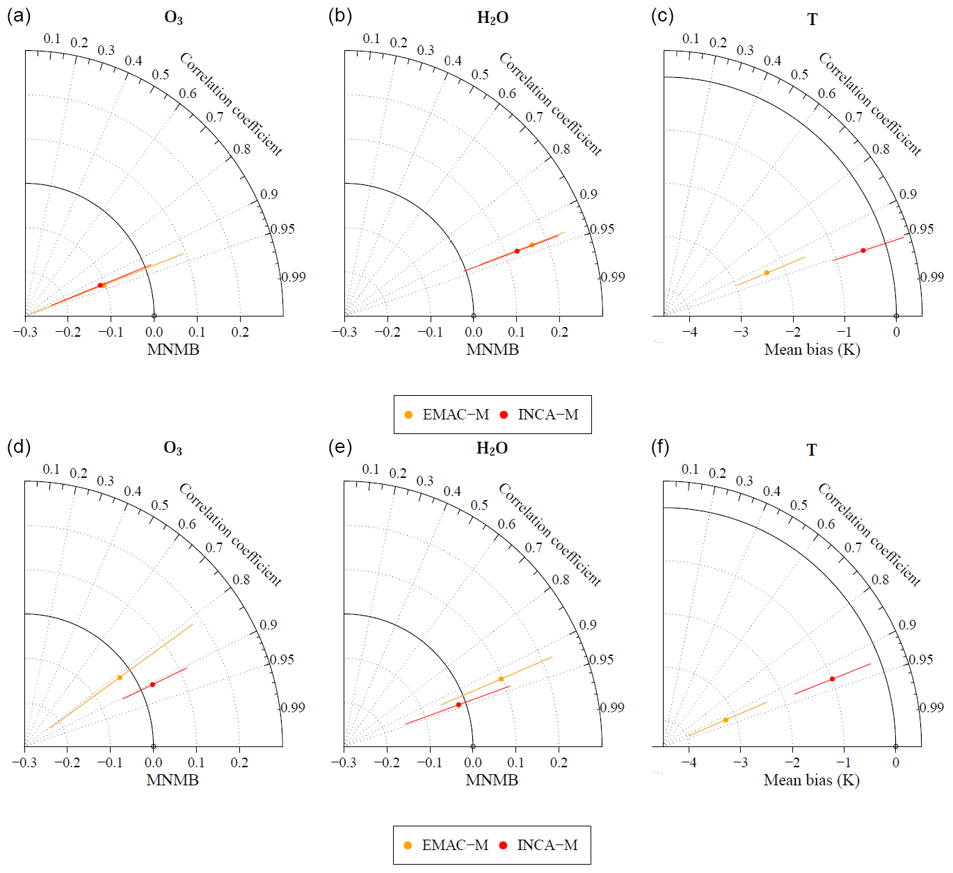
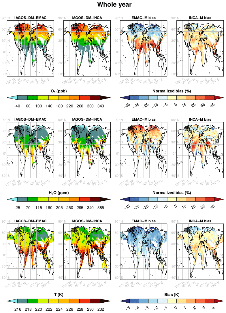
Figure A8 Annual mean climatologies for ozone, water vapor, and temperature (from top to bottom) averaged over 2000–2014 and vertically through the cruise levels. The first and second columns represent the climatologies seen by the IAGOS observations, projected onto the EMAC grid and onto the INCA grid, respectively, the latter being interpolated onto the EMAC grid afterward. The third and fourth columns show the biases between the reference simulation for each model and its corresponding gridded IAGOS product. For each grid cell, the normalized bias for the mixing ratios is calculated relatively to the average between observations and the model simulation.

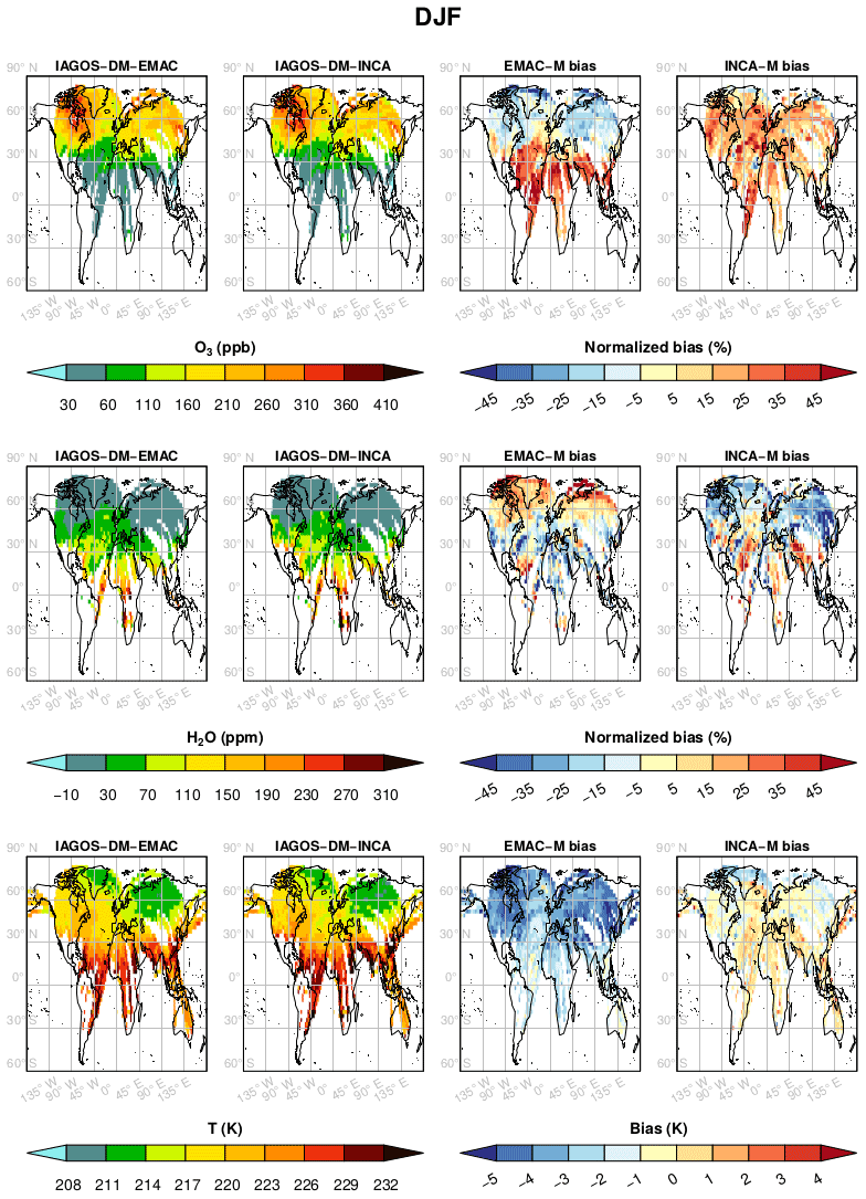
Figure A9 Same as Fig. A8 for boreal winter.

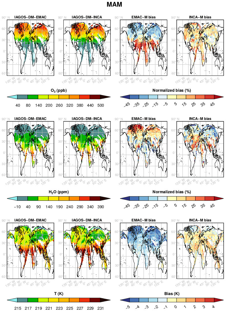
Figure A10 Same as Fig. A8 for boreal spring.

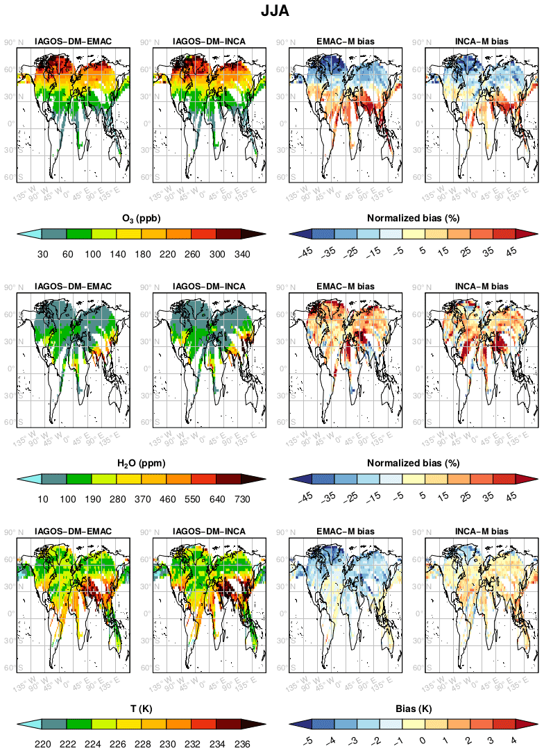
Figure A11 Same as Fig. A8 for boreal summer.

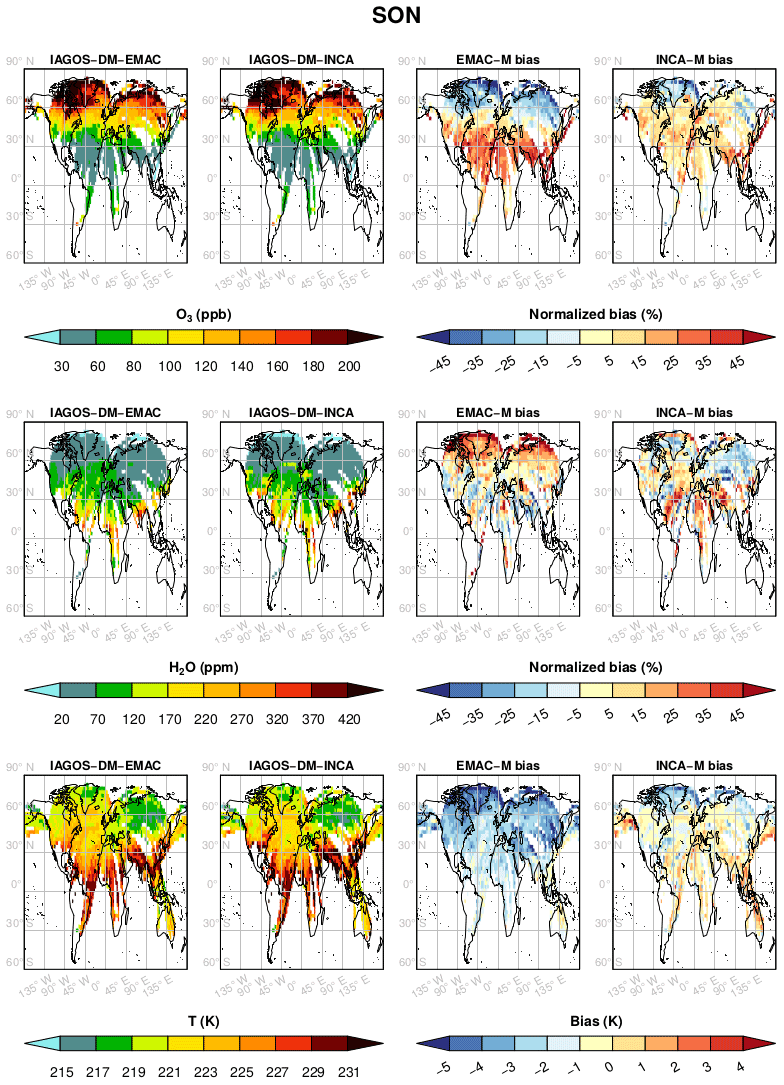
Figure A12 Same as Fig. A8 for boreal autumn.