Sensitivities of atmospheric composition and climate to altitude and latitude of hypersonic aircraft emissions

Hydrogen-powered hypersonic aircraft are designed to travel in the middle stratosphere at approximately 30–40 km. These aircraft can have a considerable impact on climate-relevant species like stratospheric water vapor, ozone, and methane and thus would contribute to climate warming. The impact of hypersonic aircraft emissions on atmospheric composition and, in turn, on radiation fluxes differs strongly depending on cruise altitude. However, in contrast to variations in the altitude of emission, differences from variations in the latitude of emission are currently unknown. Using an atmospheric chemistry general circulation model, we show that a variation in the latitude of emission can have a larger effect on perturbations and stratospheric-adjusted radiative forcing than a variation in the altitude of emission. Our results include the individual impacts of water vapor and nitrogen oxide emissions, as well as unburned hydrogen, on middle-atmospheric water vapor, ozone, and methane and the resulting radiative forcing. Water vapor perturbation lifetime continues the known tropospheric increase with altitude and reaches almost 6 years in the middle stratosphere. Our results demonstrate how atmospheric composition changes caused by emissions of hypersonic aircraft are controlled by large-scale processes like the Brewer–Dobson circulation and, depending on the latitude of emission, local phenomena like polar stratospheric clouds.

The analysis includes a model evaluation of ozone and water vapor with satellite data and a novel approach to reduce simulated years by one-third. A prospect for future hypersonic research is the analysis of seasonal sensitivities and simulations with emissions from combustion of liquefied natural gas instead of liquid hydrogen.

1 Introduction

Since the civil supersonic aircraft Concorde and Tupolev Tu-144 entered and left service (1969–2003), some time has passed. In the meantime, new projects have appeared that intend to solve the predecessors' problems, which were mainly the large cost, the significant contribution to climate warming, and the loud noise. More than a few manufactures, e.g., Boom Technology (https://boomsupersonic.com/company, last access: 5 February 2024) or Spike Aerospace (https://www.spikeaerospace.com/, last access: 5 February 2024), are on their way to deliver supersonic aircraft for commercial use. But, to our knowledge, a full-scale prototype has not been announced until today by any of the manufacturers.

Technically there are three categories of aircraft: subsonic aircraft, which fly slower than the speed of sound; supersonic aircraft, whose speed exceeds the speed of sound; and hypersonic aircraft, whose speed is at least 5 times the speed of sound. The supersonic aircraft design with the best market potential is a small-scale business jet for customers that value time greatly (Sun and Smith, 2017; Liebhardt et al., 2011). Hence, the biggest benefit of and the best sale argument for supersonic business jets are their speed and their travel time. For the same distance, the travel time of supersonic aircraft is advertised as approximately half that of subsonic aircraft. Of course, the different supersonic aircraft designs each have their specific speed and may deviate from this number. In comparison, hypersonic aircraft, which are in development but are not as technologically advanced as supersonic aircraft, fly at higher altitudes and higher speeds compared to supersonic aircraft. Hence, they reduce travel time by a factor 4 to 8 instead of 2.

Clearly, on the one hand, the aircraft industry strives to satisfy customers' needs with potential innovations like supersonic and hypersonic aircraft. On the other hand, however, the aircraft industry currently is in a transformation process to build a climate-compatible aircraft infrastructure. It easily takes decades to develop new aircraft before they can be launched on the market, and the lifetime of aircraft can also be counted in decades. Hence, the climate compatibility of new aircraft has a long-lasting effect and is therefore of utmost importance.

Generally, numerous estimates of the climate impact and the growth potential of the current aircraft industry have been published (Lee et al., 2021; Fahey et al., 2016; Pachauri and Reisinger, 2007; Pachauri, and Meyer, 2014). One of the newest estimates analyses both the climate impact and the growth potential using projections of different technological development scenarios (Grewe et al., 2021).

The impact on atmosphere and climate of potential fleets of supersonic aircraft that could replace parts of a conventional fleet has been estimated and reviewed in many – some very extensive – publications (Grewe et al., 2010; Zhang et al., 2021a; Penner et al., 1999; Matthes et al., 2022). In contrast, the first publications about atmospheric perturbation and climate impact of hypersonic aircraft have only appeared more recently (Ingenito, 2018; Kinnison et al., 2020; Pletzer et al., 2022).

Briefly summarized for supersonic and hypersonic aircraft, the non-CO₂ effect, mainly water vapor (H₂O), contributes more to climate impact with increasing altitude due to the longer H₂O perturbation lifetime and the resulting radiative forcing, and the climate impact per revenue passenger kilometers is manifold compared to that of subsonic aircraft (Grewe et al., 2010; Pletzer et al., 2022). The depletion of the ozone (O₃) layer is significant; however, the altitude dependency of the radiative forcing on emission altitude is more complex for O₃ than for H₂O (Zhang et al., 2021a, b).

Since the development of high-flying aircraft is clearly continuing, the application of mitigation options for the lowest possible climate impact during commercial use is crucial and should be fully exploited. That is not only in case these aircraft really are in use one day but also to estimate the optimization potential beforehand. The technological reality that any fuel will ultimately increase the concentration of the main climate driver, H₂O, seems inevitable since purely battery-powered aircraft are not a viable option for the distances that supersonic and hypersonic aircraft can cover in a single flight due to the batteries' weight. Taking 100 % sustainable alternative fuels provides the option of net-zero CO₂ emission flights, although availability and the degree of sustainability is likely to be a limitation for the coming decades, and non-CO₂ effects remain. Therefore, the importance of improving in-flight climate efficiency of fueled aircraft cannot be emphasized enough. The potential of climate-optimized routing for conventional aircraft (Grewe et al., 2014a, b; Sridhar et al., 2011; Matthes et al., 2012, 2020) and climate-optimized design (Grewe et al., 2017; Dahlmann et al., 2016) has been shown before. To achieve the same for high-flying aircraft, it is key to analyze sensitivities at stratospheric altitudes, i.e., the impact of aircraft emissions on atmospheric composition and climate depending on the latitude and altitude of emission.

Therefore, in this study, we performed 24 simulations and a reference simulation with the atmospheric chemistry general circulation model EMAC (ECHAM/MESSy – European Centre HAMburg general circulation model; Modular Earth Submodel System), addressing a wide range of sensitivities. The simulations include emission scenarios where H₂O, NO_x, and H₂ are emitted separately at two altitudes (30 and 38 km) and four latitude regions (southern mid-latitudes, tropics, northern mid-latitudes, north polar). The atmospheric composition changes are then used to calculate the radiative forcing with EMAC.

The paper is structured as follows. In Sect. 2, we present the EMAC model and the simulation setup, including a model evaluation with H₂O and O₃ satellite measurements and a novel approach to reduce simulation cost. Sect. 3 addresses the variations in emission with latitude and altitude and the emissions' magnitude. The direct and indirect effects of emissions, H₂O, NO_x, and H₂, on atmospheric composition are shown in Sect. 4. Section five focuses on the radiative forcing from the atmospheric composition changes followed by a discussion of atmospheric and radiative sensitivities in Sect. 6, a general discussion in Sect. 7, and a summary.

2 Methods and simulations

2.1 EMAC

We used ECHAM5/MESSy to calculate atmospheric composition changes and radiative forcing. ECHAM5 is the dynamical core of EMAC and is used to calculate the atmospheric general circulation (Roeckner et al., 2006). MESSy, version 2.54.0 of the Modular Earth Model System (Jöckel et al., 2005, 2006, 2010, 2016), extends ECHAM5 with its modular infrastructure and plug-in submodels. Overall, ECHAM5/MESSy is able to combine the atmosphere, ocean, and land domains, and the chemistry within MESSy is interconnected with these three domains. The applied atmospheric chemistry general circulation model (AC-GCM) setup is presented in the following subsection and follows the setup already presented in Pletzer et al. (2022). The model setup is from here on referred to as HS-sens.

2.2 EMAC model setup

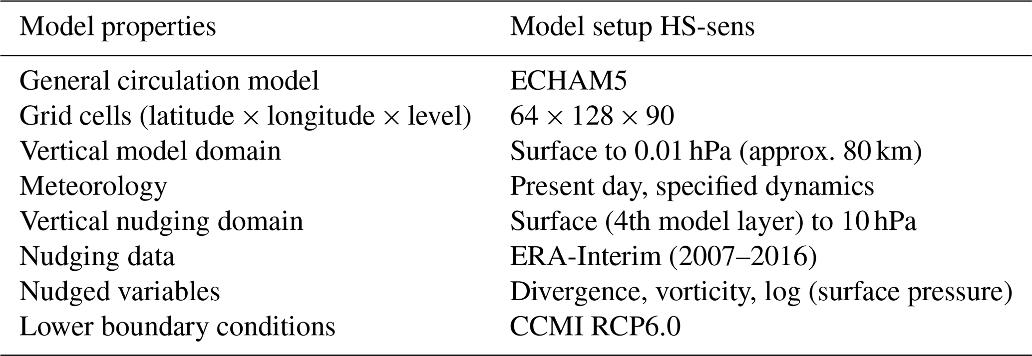
The applied horizontal resolution is T42 (triangular truncation at wave number 42) for the dynamical core, which relates to a Gaussian grid of approximately 2.8^∘ × 2.8^∘ in latitude and longitude. The vertical resolution includes 90 levels from the surface to 0.01 hPa (center of the uppermost layer) of the middle atmosphere (MA) at approximately 80 km. The complete resolution description is abbreviated as T42L90MA. The setup combines boundary conditions of 2050 surface emissions and nudging to present-day meteorology. The most relevant configuration settings are shown collectively in Table 1.

Table 1 Overview of key properties used in the model setup.

2.2.1 Specified dynamics

We used specified dynamics; i.e., we nudged towards ERA-Interim reanalysis data. This Newtonian relaxation is applied for the GCM variable divergence, with a relaxation timescale of 48 h, vorticity (6 h), and the logarithm of the surface pressure (24 h). The domain, where nudging is applied, ranges from the fourth model layer above the ground to approximately 10 hPa. Note that the impact of a 2050 meteorology would be – coarsely estimated – a 8 %–10 % strengthening of the middle-atmospheric circulation, which would reduce atmospheric perturbations from hypersonic aircraft accordingly (Sect. 7.1.2 in Pletzer et al., 2022).

2.2.2 Lower boundary conditions

The potential entry into service of hypersonic aircraft is approximately 2050. Hence, the CCMI RCP6.0 scenario was applied to simulate atmospheric conditions starting from 2050. The relevant surface emissions were included as lower boundary conditions and added to the internal tracers. Only aircraft emission scenarios were excluded.

2.2.3 Model evaluation

Temperature, O₃, and H₂O representations of the upper-troposphere–lower-stratosphere (UTLS) region in EMAC were evaluated before using aircraft measurements (Pletzer et al., 2022). We kindly ask the reader to refer to this publication for detailed information. To summarize briefly, the key message for EMAC is, firstly, a systematic cold bias of −3.8 to −2.5 K in the extra-tropics, responsible for an upward shift of the tropopause and, as a consequence, an under- and overestimation of O₃ and H₂O mixing ratios, respectively. Secondly, the Taylor correlation coefficient, estimating the correlation between observations and model results in the UTLS, is r ∼ 0.90 for H₂O and r ∼ 0.95 for O₃ and temperature. In this publication, we extend the verification region to higher altitudes, with satellite measurements published as the Stratospheric Water and OzOne Satellite Homogenized dataset (SWOOSH) by Davis et al. (2016). Further information is presented in the following Sect. 2.3.

2.3 Evaluation with satellite data (SWOOSH)

The satellite dataset SWOOSH contains H₂O and O₃ mixing ratios for the time period 1984 to 2022, and data are available for nearly all of the stratosphere and parts of the mesosphere. Here, we compare a multi-annual mean of measurements for the years 2013–2016 to two kinds of modeled stratospheric O₃ and H₂O: first to the EMAC simulations RC1SD-base-10 from Jöckel et al. (2016) with present-day meteorology and, second, to HS-sens simulation results. Note that, in contrast to the former setup, we are using boundary conditions (RCP6.0) for the year 2050. Hence, CH₄ sources, nitrous oxide, chlorine, and bromine source gases differ between the simulations, which in turn causes differences in stratospheric H₂O and O₃ concentrations. While the model setups of RC1SD-base-10 and the one from this publication, HS-sens, are largely the same, we address the differences due to the 2050 boundary conditions for O₃ and H₂O.

2.3.1 SWOOSH introduction and evaluation

The SWOOSH data consist of O₃ and H₂O measured with the satellite Aura MLS and show no gaps for the years 2013–2016. To compare, Aura MLS measurements of H₂O are quite close to the multi-instrumental mean (MIM) published by the SPARC Data Initiative (Fig. 14 in Hegglin et al., 2013, p. 11), with a continuous and moderate overestimation at all pressure levels and for both the tropics and extra-tropics. Aura MLS measurements of O₃ agree very well with the MIM at 100–5 hPa and show a small underestimation at 5–1 hPa for both the tropics and mid-latitudes (Fig. 10 in Tegtmeier et al., 2013, p. 12).

We used version 2.6 of the SWOOSH data with a horizontal resolution of 2.5^∘ and 31 vertical levels. The vertical limits are 316–0.002 hPa for H₂O and 261–0.02 hPa for O₃. The vertical resolution of SWOOSH data is 2.5–3.5 km for both O₃ and H₂O. For the comparison, EMAC data were interpolated to vertical and horizontal levels of SWOOSH data.

2.3.2 EMAC water vapor evaluation

Figure A1 in the Appendix shows the feature of increasing H₂O mixing ratios with altitude for both the model results and observations. Clearly, observation features are not as homogeneous as model results, but the general agreement is very good. The relative differences show that the magnitude of H₂O mixing ratios in the model setup with present-day meteorology is 46 ± 13 %, and that of the HS-sens model setup is 33 ± 8 % smaller than observations, on average. The largest differences appear particularly at tropical and southern latitudes in the lower stratosphere.

The increase in the average CH₄ mixing ratio of the RCP scenario between the 2010s and 2050s is about 6 %, which increases stratospheric H₂O and could explain the larger difference in observations in relation to RC1SD-base-10 simulations compared to the HS-sens model setup. Note that differences between the model and observations should, in reality, be less than what is shown in Fig. A1 since H₂O of Aura MLS is slightly overestimated at these altitudes compared to the MIM of the SPARC Data Initiative. In summary, we conclude that EMAC underestimates the H₂O mixing ratio at stratospheric altitudes for the RC1SD-base-10 results, which are based on trace gas measurements from 2013–2016. For the HS-sens model setup results, which are a projection to 2050, we expect the difference in relation to RC1SD-base-10 to originate mostly from the difference in lower boundary conditions of CH₄.

2.3.3 EMAC ozone evaluation

The multi-annual mean of O₃ shows very good agreement between the model and observations (Fig. A2). Clearly, the features look the same, and the difference in the average magnitude between observations and the model is rather small, with −5 ± 6 % and −12 ± 6 % for RC1SD-base-10 (present-day meteorology) and for the HS-sens model setup (projection to 2050), respectively. For the RC1SD-base-10 scenario SWOOSH observations are within the standard deviation of model simulations. The largest deviations appear in the same areas for both model setups, RC1SD-base-10 and HS-sens. They are at the tropics and southern mid-latitudes at 100 hPa and at polar regions at higher altitudes.

O₃ mixing ratios are expected to increase over time compared to the 2010s since emissions of chlorine and bromine source gases stagnate significantly (World Meteorological Organization et al., 2019, 2015). Hence, the difference, when comparing measurements of the 2010s and model results with boundary conditions for the 2050s, is to be expected. Therefore, we conclude that EMAC shows a very good agreement of stratospheric O₃ mixing ratios compared to observations for both HS-sens model results and the RC1SD-base-10 scenario.

2.4 Enhancing the efficient use of computing resources

The simulations with Earth system models are very time and cost intensive, with a high energy consumption. Therefore, we introduce a method which reduces the number of simulated years of the spin-up phase to three-fifths.

Finite computer resources were mentioned before by Hasselmann et al. (1993), along with the related “cold-start” error. The cold-start problem refers to coupled atmosphere–ocean simulations that are started close to the present and not early at the beginning of anthropogenic greenhouse gas emission, which eventually generates a significant error in the forcing results due to the too-short spin-up phase.

Our computing challenge has an analogy to the above described coupled atmosphere–ocean GCMs that are normally run for very long timescales and, therefore, have a large reduction potential. Here, we run an atmospheric–chemistry GCM for many simulations with variations in the location of emitted trace gases at stratospheric altitudes, each requiring a significant spin-up time (Fig. 3 in Pletzer et al., 2022).

With our applied speed-up method, we achieve equilibrium in terms of the multi-annual mean faster and hence are able to reduce the simulated years to two-thirds. The method is the following. We estimate the equilibrium mass change of a species due to an emission and apply an increase in the emissions by a factor s in the first year so that this equilibrium mass change is approximately reached after a 1-year simulation instead of a 10-year spin-up. The factor s is calculated using a one-dimensional differential equation containing the H₂O perturbation lifetime τ and is therefore dependent on altitude (Fig. A3). In a quasi-steady state with a stratospheric H₂O mass perturbation X (kg), an annual emission E (kg yr⁻¹), and a perturbation lifetime τ (years), we obtain

$$\begin{array}{}\text{(1)}& \mathrm{0}={\displaystyle \frac{\mathit{\delta }X}{\mathit{\delta }t}}=E-{\displaystyle \frac{\mathrm{1}}{\mathit{\tau }}}X,\end{array}$$

or, in other words,

$$\begin{array}{}\text{(2)}& X=\mathit{\tau }E.\end{array}$$

To obtain the value of s we solve the differential equation for the evolution of the stratospheric H₂O mass change to Y for an emission sX:

$$\begin{array}{}\text{(3)}& {\displaystyle \frac{\mathit{\delta }Y}{\mathit{\delta }t}}=sE-{\displaystyle \frac{\mathrm{1}}{\mathit{\tau }}}Y,\end{array}$$

with the boundary conditions $Y(t=\mathrm{0})=\mathrm{0}$ and $Y(t=\mathrm{1})=\mathit{\tau }E$. The solution of the differential equation that fulfills the first boundary condition is then

$$\begin{array}{}\text{(4)}& Y\left(t\right)=s\mathit{\tau }E\left(\mathrm{1}-e^{-\frac{\mathrm{1}}{\mathit{\tau }}t}\right).\end{array}$$

In combination with the second boundary condition, this gives us

$$\begin{array}{}\text{(5)}& s={\displaystyle \frac{\mathrm{1}}{\mathrm{1}-e^{-\frac{\mathrm{1}}{\mathit{\tau }}}}}.\end{array}$$

Hence, if we estimate s with a Taylor approximation, we obtain the perturbation lifetime of τ. However, if we enhance the emission by this factor, we additionally have to consider the loss during the first year with a factor of 0.5, which applies for τ between 2 to 5 years.

$$\begin{array}{}\text{(6)}& s\approx \mathit{\tau }+\mathrm{0.5}\end{array}$$

We used H₂O perturbation lifetime values at stratospheric altitudes from Grewe and Stenke (2008) and Pletzer et al. (2022) as initial values and interpolated and extrapolated to altitudes of 30 and 38 km, respectively. Since the slopes of linear and quadratic extrapolation (35–42 km) were either very steep or too curved, we used the average of both values. Using the interpolated τ values, we calculated s using Eq. (6).

The process during the model runs is as follows. After the first year of simulation, where we enhanced the emissions by the factor s, the initial values of trace gases are emitted for the following years in the simulation. The first year, on the one hand, ensures that atmospheric composition changes reach multi-annual equilibrium faster. On the other hand, by limiting the enhancement to the first year, the final mass perturbation is not disturbed since the atmospheric lifetime of perturbations is shorter than the spin-up phase. For validation, we compared the mass perturbation of H₂O above the tropopause over time for the different scenarios, which is shown in Fig. A4. Please refer to Sect. 3.3 for a comparison of scenarios and validation of multi-annual mean equilibrium. To summarize briefly, with the altered spin-up, we reduced the consumption of the normally used computational resources to two-thirds, with minimal error potential for all 24 perturbation simulations.

3 Emission scenarios

We use total annual emissions of a potential fleet of hypersonic aircraft that consist of H₂O, NO_x, and H₂ emissions. These emissions were presented before by Pletzer et al. (2022, p. 12) and originate from the “HIgh speed Key technologies for future Air transport – Research and Innovation cooperation scheme” project, abbreviated as HIKARI (Blanvillain and Gallic, 2015). H₂O emissions occur as a product of H₂ combustion. Nitrogen oxide is produced at high temperatures during combustion and originates from ambient-air (N₂ and O₂). Complete combustion of H₂ is very difficult to achieve, and, in this dataset, it is estimated that 10 % of the H₂ fuel remains unburned. These values exclude tropospheric and subsonic emissions and are from altitudes above 18 km, referring to exhaust during cruise phase. The following two subsections contain information on the location and magnitude of all 24 perturbation scenarios.

3.1 Emission locations of perturbation scenarios

The emission scenarios are not based on aircraft route networks but are box emissions that are varied in latitude and altitude (Fig. 1). Altitudes of emission are 30 and 38 km. Note that the height of the box, where the exhaust is emitted, is approximately 1 km. Therefore, it is rather an altitude range with 30–31 and 38–39 km, where trace gases are emitted. Each latitude region of emission spans 30^∘. They are southern mid-latitudes at 60–30^∘ S, northern tropics at 0–30^∘ N, northern mid-latitudes at 30–60^∘ N, and north polar latitudes at 60–90^∘ N. Clearly, south polar and southern tropics are missing. We refrained from including these two regions for three reasons. First, aircraft barely fly at southern polar regions since most direct routes between city pairs do not cross there. Therefore, they are not as important as an emission location. Second, since we included northern tropics, we passed on southern tropics since they show very similar dynamic and chemical conditions in the stratosphere. However, we included southern mid-latitudes to quantify the impact on atmospheric composition and climate in the Southern Hemisphere. Third, with this approach, we could reduce the use of computational resources further.

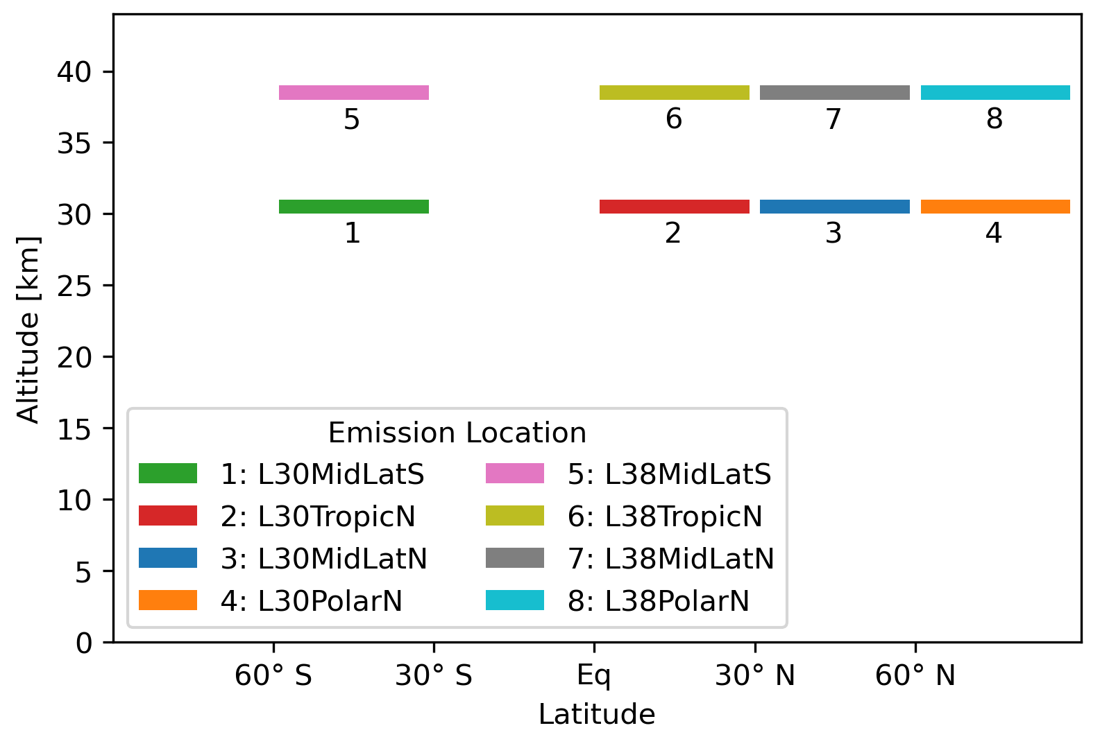
Figure 1 Altitude and latitude regions of emission of, in total, eight emission locations. For three types of emission, these sum to 24 emission scenarios.​​​​​​​

3.2 Emission magnitude of perturbation scenarios

During simulations, the individual trace gases (Table 2) are continuously emitted in the described altitude and latitude regions and, with that, are introduced to physical and chemical processes in the AC-GCM. We aim at identifying the impact on the atmosphere from the cruise phase and hence do not consider other phases such as take off and landing in this idealized simulation setup.

Table 2 Emission scenarios listed by the kind of emission and magnitude.

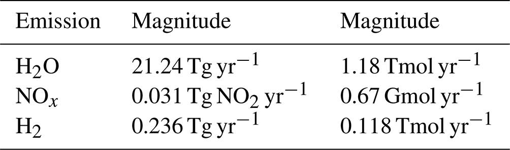
For each emitted trace gas (H₂O, NO_x, H₂) there are a total of 8 simulations, which sum up to 24 simulations in total. The annual magnitude of emitted trace gases is 21.24 Tg of H₂O, 0.031 Tg NO₂ of NO_x, and 0.236 Tg of H₂. These values are based on emissions of the aircraft design LAPCAT-PREPHA (Long-Term Advanced Propulsion Concepts and Technologies; Programme de REcherche et de technologie sur la Propulsion Hypersonique Avancée) and are based on approximately 200 flights per day with this aircraft. Why individual emission is appropriate here, even though trace gases are emitted simultaneously during aircraft operation, is discussed in Sect. 7.4.

3.3 Timeline and validation

To validate the multi-annual mean equilibrium of atmospheric composition in the context of the speed-up, presented in Sect. 2.4, we compare the timeline of H₂O mass perturbations. Of the emitted trace gases, H₂O has the longest perturbation lifetime and therefore serves as the medium to verify multi-annual mean equilibrium. Figure A4 shows the temporal evolution of H₂O mass perturbation. Three phases can be seen. (1) The first year shows a sharp increase due to the applied speed-up factor s (gray-shaded area). (2) From 2008 to 2012, some scenarios overshot equilibrium values with the end of the first year, e.g., 30 km, 60–90^∘ N, and leveled off to equilibrium values. (3) Other scenarios continued to build up, e.g., most scenarios at 38 km, before reaching equilibrium (green shaded), at latest in 2013.

The different behavior most probably originates from latitudinal differences in H₂O perturbation lifetime, which were not included in the interpolation and extrapolation in Sect. 2.4. The error potential should not be significant since the time to equilibrate is sufficient for all scenarios, and multi-annual mean equilibrium is reached at latest in 2013. Clearly, equilibrium is not reached within 1 year as assumed, and total spin-up until equilibrium amounts to 6 years since latitudinal differences had to be taken into account as well. However, without the spin-up method, we would require 10 years (Fig. 3 in Pletzer et al., 2022), and, hence, we could reduce the spin-up computing time by 40 % and the total computing time by approximately 33 %.

4 Atmospheric composition changes

In this section we present, first, as an overview of simulation results, the impact on the two most important climate active gases in the context of hypersonic aircraft exhaust, O₃ and H₂O, and, second, the direct and indirect effects on atmospheric composition by the emission of H₂O, NO_x, and H₂ for all 24 scenarios. Third, we address CH₄ and H₂O perturbation lifetime. Note that all presented data in this section are based on multi-annual mean model results with both, specified meteorology (2013–2016) and 2050 source gas emissions.

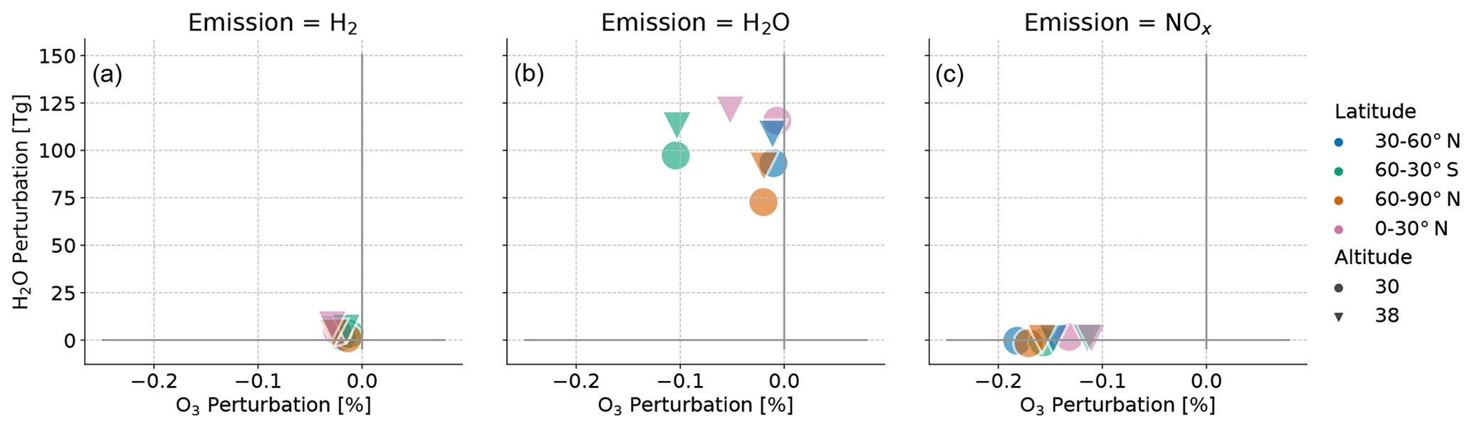
Figure 2 Overview of H₂O and O₃ changes for all 24 simulations grouped by initial emission of H₂ (a), H₂O (b), and NO_x (c). Colors refer to the latitude region of emission (southern mid-latitudes, northern tropical latitudes, northern mid-latitudes, north polar latitudes), and markers refer to altitude of emission. Please refer to Table 4 for statistical significance.

Figure 2 shows the H₂O mass perturbation and relative O₃ changes above the meteorological tropopause (WMO) grouped by emitted species. Hydrogen (H₂) emission has a comparably small effect on both H₂O and O₃. Relative O₃ changes range from −0.01 % to −0.03 %, with a decrease for all H₂ emission scenarios. The effect is larger for the higher-altitude scenarios. H₂O changes are not larger than 8 Tg, with maximum values for the northern-tropic emission scenario at 38 km. H₂O emission has a large effect on H₂O mass perturbation in all scenarios, with a range of 73–121 Tg. Values for higher-altitude and lower-latitude scenarios are particularly large. Relative O₃ change is rather small, except in the southern mid-latitudes, where O₃ depletion is approximately 0.1 % for both altitudes. The altitude of emission has a large effect on emission at the tropics, and emission at 38 km has a significantly larger impact on ozone. NO_x emission has the lowest effect on H₂O mass perturbation. The range of H₂O changes is −1.6 to 1.7 Tg, and all higher-altitude emission scenarios show an increase with medium values. In contrast, the lower-altitude emission scenarios show larger values but differ in terms of their increase and decrease. Relative O₃ change due to NO_x emission is larger than most other emission scenarios, with a range of −0.11 % to −0.18 %. The largest values appear at northern mid-latitudes and polar regions at 30 km.

The following subsections are further divided into “Direct effects” and “Indirect effects”. The former relates to the emission and its effect on the same molecular atmospheric compound, e.g., H₂O emission on H₂O trace gas concentrations. The latter includes indirect effects on other atmospheric compounds like CH₄ or O₃. The shaded box in each subfigure represents the altitude of emission. Hatched areas represent a p value larger than that written in the title of each subplot (Table 3).

Table 3 Markers for probability levels of significance test.

4.1 Water vapor emission

4.1.1 Direct effects

Figure 3 shows the H₂O perturbation in parts per million volume for the H₂O emission scenarios. When comparing the altitudes of 38 and 30 km, which are the first and second lines, respectively, the H₂O mixing ratios are generally higher for the former. H₂O emissions at low latitudes are distributed across both hemispheres. H₂O emissions at higher altitudes are, to a significantly larger extent, confined to one hemisphere. The threshold for failing the t test is exceeded at and below the tropopause region.

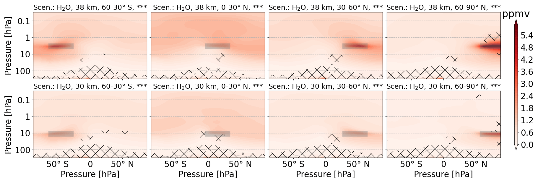
Figure 3 Zonal mean of H₂O perturbation (volume mixing ratio, ppmv) for scenarios where H₂O is emitted. The first and second rows refer to 38 and 30 km altitudes of emission, respectively. Columns represent the latitude region of emission. The emission regions are shaded in gray. Lines indicate statistically insignificant results, and the probability level is written in the title of each subplot.

4.1.2 Indirect effects

Ozone

In total, the H₂O emission causes O₃ depletion, especially at southern latitudes (Fig. 2). In Fig. 4, the O₃ perturbation (volume mixing ratio) is divided into layers of O₃ decrease (above 3 hPa and below 10 hPa) and O₃ increase (3–10 hPa) in all subfigures. For emission at 38 km, the upper layer of O₃ decrease seems to be strengthened. For emission at 30 km, the layer of O₃ increase overlaps with the emission region and seems to be weakened, especially for H₂O emission from 0–30^∘ N. The threshold for failing the t test has, in general, a large variation and appears at the interface of O₃ increase and O₃ decrease regions, the tropopause and polar regions. The largest values of O₃ increase are situated in the tropics for all scenarios. In contrast, the largest values of O₃ decrease move with the emission location.

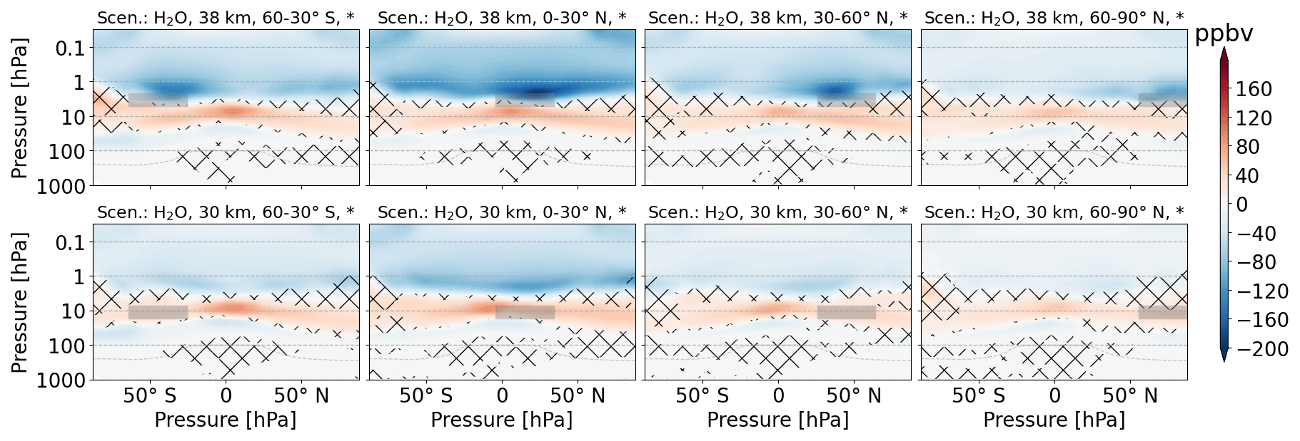
Figure 4 Zonal mean of O₃ perturbation (volume mixing ratio, ppbv) for scenarios where H₂O is emitted. The first and second rows refer to 38 and 30 km altitudes of emission, respectively. Columns represent the latitude region of emission. The emission regions are shaded in gray. Lines indicate statistically insignificant results, and the probability level is written in the title of each subplot.

Hydrogen

The H₂O emission has a significant effect on H₂ (Fig. A7) at the top of the modeled atmosphere (around 80 km). In general, the H₂ perturbation patterns are very similar, with a broad layer at high latitudes and a smaller width at middle to low latitudes. The magnitude, however, is larger for emission scenarios with low latitudes and the higher emission altitude (38 km).

Methane

The impact of H₂O emission on CH₄ shows complex patterns, with areas of increase and decrease, and the multi-annual variability is clearly large since the t test restricts confidence in many areas (Fig. 5). It is common knowledge that OH oxidizes CH₄ and adds to H₂O concentrations in the stratosphere. Additionally, it was shown that emission of H₂O eventually increases CH₄ oxidation (Pletzer et al., 2022). Overall, H₂O emissions reduce CH₄ concentrations the most compared to emissions of NO_x and H₂ (this changes when normalized to the number of emitted molecules). The features for emission at southern mid-latitudes are very similar, with a decrease from 100 to 10 hPa and an additional decrease around the emission location of the higher-altitude scenario. H₂O emission at northern tropics causes a widespread CH₄ depletion with a larger impact for the higher-altitude emission. A CH₄ increase is visible in the tropics at 10 hPa for 30 km emission. For 38 km, the area with CH₄ increase, where p ≤ ​​​​​​​0.05, is barely visible. Northern mid-latitude emission of H₂O shows features similar to southern mid-latitude emission, but the decrease is at slightly higher altitudes. Areas of increase and decrease seem to have switched locations. This statement should be taken with caution since not all areas included in the comparison fulfill the t-test criteria (i.e., the error probability that means are not different is larger than 5 %). North polar emission scenarios are very similar to the north mid-latitude emission scenarios. However, perturbations of volume mixing ratios are generally smaller.

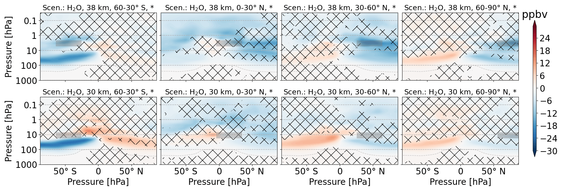
Figure 5 Zonal mean of CH₄ perturbation (volume mixing ratio, ppbv) for scenarios where H₂O is emitted. The first and second rows refer to 38 and 30 km altitudes of emission, respectively. Columns represent the latitude region of emission. The emission regions are shaded in gray. Lines indicate statistically insignificant results, and the probability level is written in the title of each subplot.

4.2 Nitrogen oxide emission and ozone perturbation

4.2.1 Direct effects

The emitted NO_x is, compared to H₂O, more confined to the emission region. First, the NO_x perturbation maximum is clearly located at the altitude and latitude of emission – other maxima are not visible. Second, the multi-annual mean of emission scenarios and the reference scenario are different for most areas in direct proximity to the emission location (hatched area). NO_x changes are more distributed for low-latitude emission scenarios. The vertical distribution shows downward transport for high latitudes and upward transport for low latitudes, depending on the latitude of emission. A correlation plot of significant NO_x and O₃ changes (Fig. A9) shows a nearly linear correlation for altitudes from the surface to 4 hPa, with a tendency towards saturation for larger NO_x perturbations in the lower-altitude emission scenarios. For altitudes from 4 to 0.01 hPa the correlation is curvilinear, and the NO_x emission scenarios show a larger range of values compared to the lower-altitude range. Here, the sensitivity to the altitude and latitude of emission is very large.

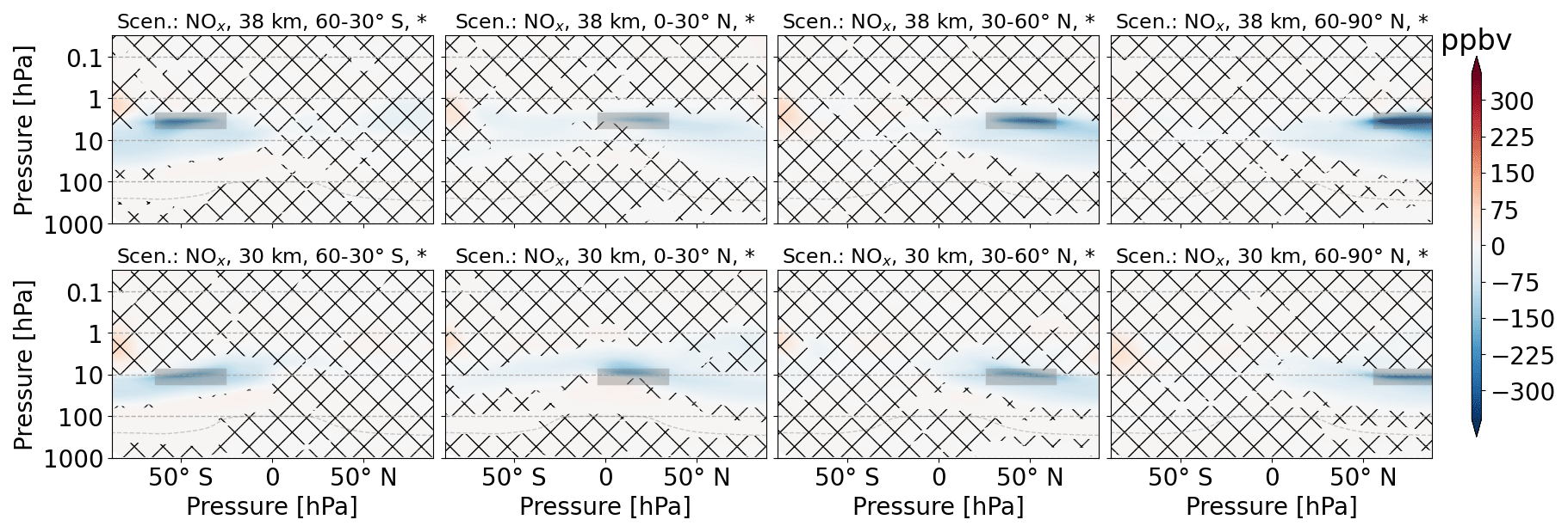
Figure 6 Zonal mean of O₃ perturbation (volume mixing ratio, ppbv) for scenarios where NO_x is emitted. The first and second rows refer to 38 and 30 km altitudes of emission, respectively. Columns represent the latitude region of emission. The emission regions are shaded in gray. Lines indicate statistically insignificant results, and the probability level is written in the title of each subplot.

Since the correlation of O₃ and NO_x perturbation is well known, we include the O₃ perturbation as a direct effect. When comparing Figs. 6 and A10, the similarity is clearly visible. Areas of NO_x increase overlap with areas of O₃ decrease. Additionally, we see areas of O₃ increase below areas of O₃ decrease at southern mid-latitude and northern tropic emission scenarios. Note that the magnitude is much smaller, and results are clearly significant. For northern mid-latitude scenarios, these are barely visible in the tropics, and for north polar emission scenarios, they are not visible.

4.2.2 Indirect effects

Overall, indirect effects of NO_x emission on H₂O, H₂, and CH₄ are basically insignificant for most areas. For some scenarios, significant areas appear for tropospheric and lower-stratospheric altitudes, largely depending on which hemisphere NO_x was emitted in (Figs. A11, A12, A13).

4.3 Hydrogen emission

4.3.1 Direct effects

The increase in atmospheric concentrations of H₂ by H₂ emission peaks at the emission location (Fig. 7). The perturbation pattern looks very similar to H₂O perturbation from H₂O emission and is therefore most probably dominated by transport, i.e., the Brewer–Dobson circulation, instead of photochemistry.

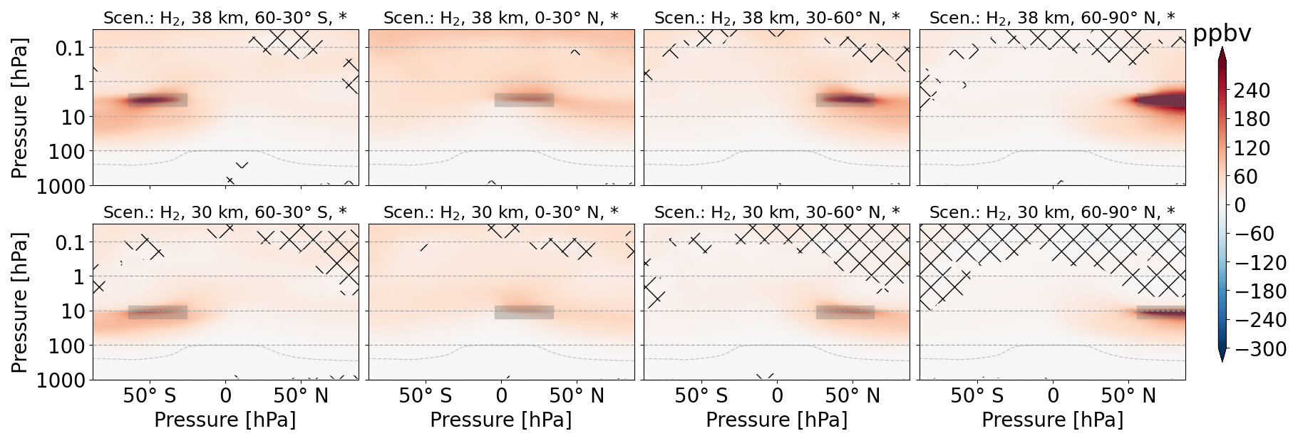
Figure 7 Zonal mean of H₂ perturbation (volume mixing ratio, ppbv) for scenarios where H₂ is emitted. The first and second rows refer to 38 and 30 km altitudes of emission, respectively. Columns represent the latitude region of emission. The emission regions are shaded in gray. Lines indicate statistically insignificant results, and the probability level is written in the title of each subplot.

4.3.2 Indirect effects

The EMAC results show that H₂ emissions at 38 km generally and for the tropics at 30 km statistically significantly reduce the O₃ abundance in the upper stratosphere (0.1–1 hPa). It is known that, above 40 km, the HO_x cycle starts to dominate the O₃ depletion instead of the NO_x cycle (Zhang et al., 2021a; Matthes et al., 2022).

Maximum values of H₂O perturbation are approximately 5 % of the H₂O perturbation of the direct H₂O emission scenarios. Apart from the magnitude, the features are very similar, which again suggests that transport dominates these perturbations (Fig. A15). The largest perturbations appear for the higher-altitude scenarios and the low-latitude scenarios. A correlation plot shows that statistically significant H₂O changes due to H₂ emission show different orders of magnitude depending on the hemisphere, with larger gradients appearing rather in the Southern Hemisphere. Clearly, high-latitude and low-altitude emission scenarios show smaller H₂O changes and again suggest a dominant role of transport in the perturbation lifetime.

CH₄ perturbation patterns are mostly not statistically significant (Fig. A16).

4.4 Methane, water vapor perturbation lifetime, and overview of relative changes

4.4.1 Methane and methane lifetime

The tropospheric and whole-model-domain CH₄ lifetimes of all emission scenarios are 8.39 and 9.54 years on average, respectively. We used the following equation to calculate both the tropospheric and whole-domain CH₄ lifetimes, ${\mathit{\tau }}_{{\mathrm{CH}}_{\mathrm{4}}}$:

$$\begin{array}{}\text{(7)}& {\mathit{\tau }}_{{\mathrm{CH}}_{\mathrm{4}}}\left(t\right)={\displaystyle \frac{\sum _{b\mathit{ϵ}B}{M}_{{\mathrm{CH}}_{\mathrm{4}}}^b\left(t\right)}{\sum _{b\mathit{ϵ}B}{k}_{{\mathrm{CH}}_{\mathrm{4}}}^b\left(t\right)\cdot {\left[\mathrm{OH}\right]}^b\left(t\right)\cdot M_{{\mathrm{CH}}_{\mathrm{4}}}^b\left(t\right)}}.\end{array}$$

$M_{{\mathrm{CH}}_{\mathrm{4}}}^b$ is the CH₄ mass, [OH]^b is the concentration, and $k_{{\mathrm{CH}}_{\mathrm{4}}}^b$ is the reaction rate of CH₄ + OH in grid box b. B is the set of all grid boxes.

Equation (7) was applied to calculate the tropospheric CH₄ lifetime for different EMAC model setups (Fig. 16 in Jöckel et al., 2016). The results show an average value over all setups of 8.0 ± 0.6 for the years 2000–2004, which, according to the authors, is on the lower end of a set of values from other publications.

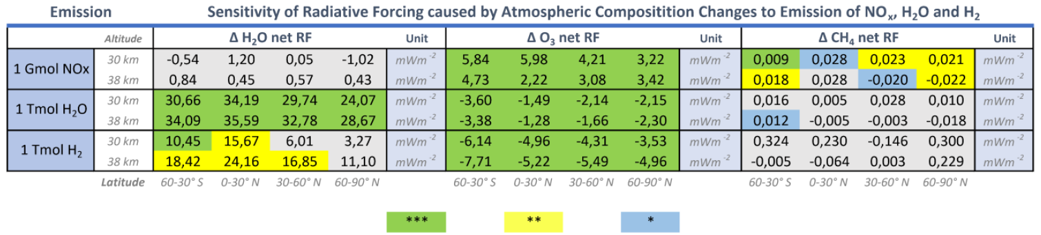
Table 4 Sensitivities of atmospheric composition changes, water vapor in teramole (ΔH₂O), relative ozone change in teramole (ΔO₃), and relative change of whole-model-domain methane lifetime ($\mathrm{\Delta }{\mathit{\tau }}_{{\mathrm{CH}}_{\mathrm{4}}}$) to emission of H₂O, NO_x, and H₂ depending on the altitude and latitude of emission. Asterisks refer to statistical significance (Table 3).

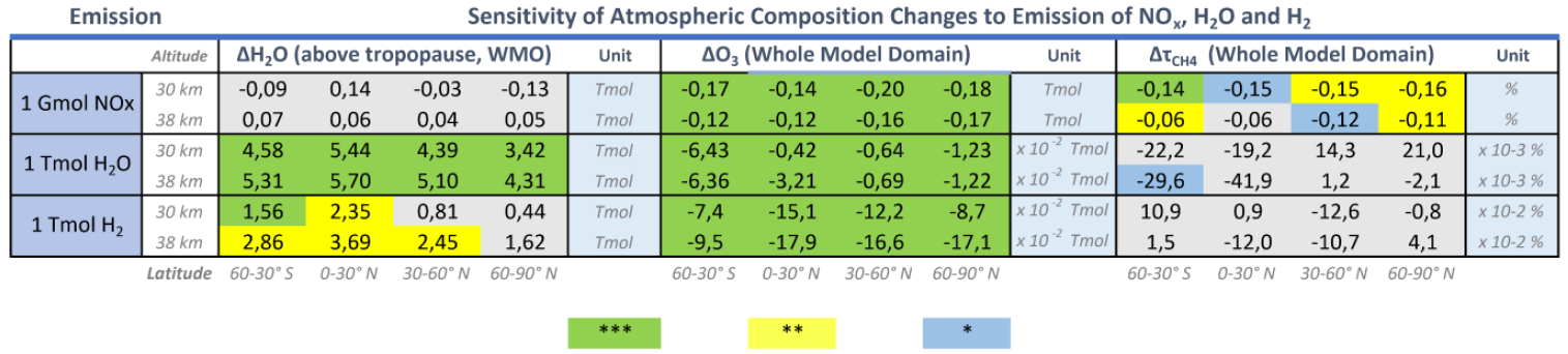
Figure A5 shows the CH₄ lifetime (Fig. A5a) and H₂O mass perturbation (Fig. A5b) in relation to the relative hydroxyl radical mass change. CH₄ lifetime changes of H₂ emission scenarios are quite close to the reference scenario, and a clear trend is not visible. H₂O emission scenarios show a clear correlation between OH increase and CH₄ lifetime decrease, with an increase or only a small change at higher-northern-latitude and lower-altitude scenarios and a decrease in CH₄ lifetime for southern- and tropical-latitude scenarios (Table 4). An average over all emission scenarios per emission type shows an increase in the relative hydroxyl and hydroperoxyl mass, mostly in the middle atmosphere (Table A2). This explains the decreasing global CH₄ lifetime for H₂O with a more efficient CH₄ oxidation due to an increase in OH (Fig. A5b).

NO_x emission scenarios, which show small OH perturbations close to zero, also show the largest reduction in ${\mathit{\tau }}_{{\mathrm{CH}}_{\mathrm{4}}}$ with two altitude clusters (green-shaded ellipses). As an addition, Fig. A6 in the Appendix shows the tropospheric CH₄ lifetime, which shows very similar trends for NO_x emission scenarios compared to the whole-model-domain CH₄ lifetime. According to the literature, two pathways of tropospheric chemistry connect NO_x and OH concentrations. On the one hand, HO₂-to-OH recycling is sped up by NO and eventually increases OH. On the other hand, NO₂ oxidation reduces OH concentrations and increases nitric acid (HNO₃) concentrations (Ehhalt et al., 2015, p. 245). Note that tropospheric OH concentrations are only slightly increased for NO_x emission scenarios (Table A2). The abovementioned processes might not allow large perturbations of OH to build up even though the effects on CH₄ lifetime are the largest in all scenarios.

In the troposphere, H₂O emission and NO_x emission scenarios show an inverse trend with a tropospheric CH₄ lifetime increase (Fig. A6) combined with a tropospheric hydroxyl decrease (Table A2) for the former and a tropospheric CH₄ lifetime decrease combined with a tropospheric hydroxyl increase for the latter. In summary, the important processes for global CH₄ lifetime take place in the troposphere for NO_x scenarios and in the middle atmosphere for H₂O emission scenarios.

4.4.2 Water vapor perturbation lifetime

Figure 8 shows an increase in H₂O perturbation lifetime with altitude. Values at tropospheric altitudes range from approximately 1 h to half a year. Generally, the H₂O perturbation lifetime is longest at tropical regions and high altitudes and gets less at higher latitudes and lower altitudes. The lifetime range at stratospheric altitudes is large, from 1 month to 5.5 years, which includes the extension that is based on this work. We used our data to extend the altitude dependency of H₂O perturbation lifetime in the existing literature to higher altitudes. Grewe and Stenke (2008) published H₂O perturbation lifetime from the surface to approximately 20 km (50 hPa). We extended the range up to approximately 40 km (3 hPa). The transport of low-latitude, high-altitude H₂O emissions to the high latitudes of the troposphere along the shallow and deep branches of the Brewer–Dobson circulation takes the longest time. Hence, transport of H₂O perturbations dominates the perturbation lifetime for both the previous and the extended altitudes. Pletzer et al. (2022) showed that photochemistry does not reduce total H₂O perturbations at 26 and 35 km cruise altitude. We report that perturbation lifetimes continue to increase with altitude for all latitudes and that photochemistry does not deplete total H₂O perturbations for emissions up to 38 km.

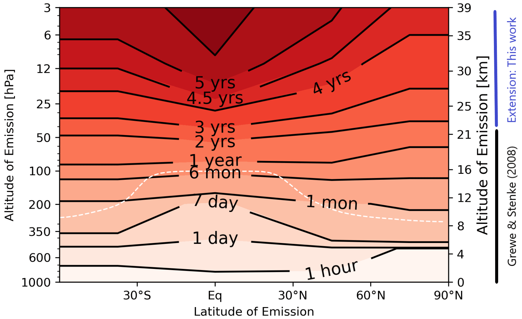
Figure 8 Reproduced from Grewe and Stenke (2008, Fig. 6a), with permission from the authors, who provided the data. The figure shows the water vapor perturbation lifetime for the original pressure levels (1000–52 hPa) and the extended pressure levels (52–3 hPa) depending on latitude. The vertical regions are marked next to the right y axis with black and blue lines, respectively.

4.4.3 Overview on atmospheric composition

For a quick-look overview of sensitivities, we present Table 4, which shows the effect of one gigamole or teramole of H₂O, NO_x, and H₂ emission on H₂O (above the tropopause), whole-model-domain O₃, and whole-model-domain CH₄ lifetime ${\mathit{\tau }}_{{\mathrm{CH}}_{\mathrm{4}}}$. We added background colors of blue, yellow, and green, indicating that the values differ from zero with a probability of 95 %, 99.9 %, and 99.99 %. The impact of NO_x, H₂O, and H₂ emission on O₃ is statistically significant with 99.99 % confidence for all 24 sensitivities. For sensitivities of H₂O and CH₄ lifetime, 13 and 8 out of 24 means are different to the reference with at least 95 % confidence, respectively.

Water vapor perturbation in the middle atmosphere

The term stratospheric H₂O is quite common. Since the HS-sens model setup includes parts of the mesosphere, we prefer to use the term mid-atmospheric H₂O. For H₂O emission, the sensitivity of mid-atmospheric H₂O increases clearly with altitude and is higher for lower-latitude emission scenarios, which is also shown in Fig. 8. The impact of H₂ emission on mid-atmospheric H₂O is very similar and increases with altitude and is larger for lower latitudes. The order of magnitude of changes per molecule of emitted species shows that a molecule of H₂ is roughly 50 % as effective in enhancing the mid-atmospheric H₂O concentration as a molecule of emitted H₂O (Tables 4, A1). The relevant reactions include both the loss and production of H₂O. Chemically, the production is initiated directly by the reaction H₂ + OH → H₂O + H and indirectly by HO₂ + OH → H₂O + O₂. The latter is facilitated by the general increase in HO_x and is included in a H₂O–HO_x cycle via the reaction H₂O + O(¹D) = 2OH. Increased oxidation, e.g., methane and nitric acid oxidation, contributes a small amount as well. The net production of H₂O is briefly discussed in Sect. 7.2.

Whole-model-domain ozone perturbation

Generally, all three types of emissions cause O₃ depletion. However, the effect of NO_x emission on whole-model-domain O₃ is 2 and 3 orders of magnitude larger compared to H₂ and H₂O emission, respectively. Hence, a NO_x molecule is roughly 3 to 4 orders of magnitude more efficient in reducing the stratospheric O₃ burden than H₂ or H₂O. Interestingly, while in absolute values the H₂ emissions are of minor importance to the O₃ depletion, the average effectiveness in destroying O₃ is roughly 5–6 times larger for H₂ than for H₂O (Table 4).

Whole-model-domain methane lifetime change

The number of significant results in terms of CH₄ lifetime changes is low compared to atmospheric sensitivities of H₂O or O₃. CH₄ lifetime changes of NO_x emission scenarios are lower at higher altitudes and show ranges between −0.06 % and −0.16 % per gigamole of NO_x emission. Per-molecule-CH₄ lifetime changes of H₂O emission scenarios are 4 to 5 orders of magnitude smaller compared to NO_x emission scenarios. Note that CH₄ lifetime in H₂O and NO_x emission scenarios clearly shows a linear trend or clusters depending on altitude, respectively, while H₂ emission scenarios do not show a clear trend (Fig. A5).

5 Radiative forcing

We used the atmospheric changes of the radiatively active gases, H₂O, O₃, and CH₄, to calculate the stratospheric-adjusted radiative forcing (total net RF) at the tropopause (about 180 hPa).

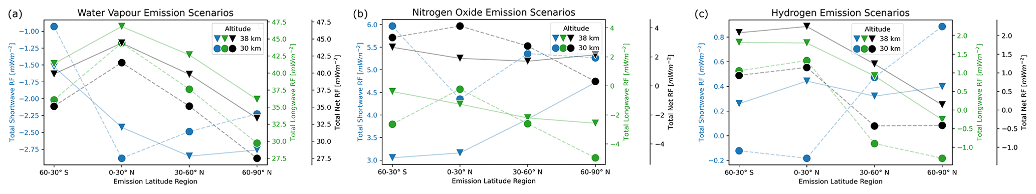
Figure 9 The total shortwave, longwave, and net radiative forcing in blue, green, and black, respectively, for water vapor (a), nitrogen oxide (b), and hydrogen (c) emission scenarios due to atmospheric composition changes in water vapor, ozone, and methane. For different altitude emission scenarios, refer to markers. Latitude regions of emission are aligned on the x axis.

In Fig. 9, we present the total net RF, which shows the total shortwave (SW), total longwave (LW), and total net RF grouped by emission, aligned by latitude, and marked by altitude of emission. Here, total refers to the combined effect of RF due to H₂O, O₃, and CH₄ changes. In the following subsections, we address the individual H₂O, O₃, and CH₄ altitude and latitude dependencies of RF and the relation of RF to atmospheric composition changes.

Comparing the magnitude, the H₂O emission scenarios show the largest total net RF, followed by NO_x and H₂ emission scenarios.

H₂O emission scenarios all have a negative total SW RF (blue), which is smallest at southern mid-latitudes. The total LW RF (green) is largest for tropical and smallest for north polar emission scenarios. The high-altitude emission scenarios show a larger total LW RF for all latitudes.

NO_x emission scenarios show a positive total SW RF, which is larger for the lower-altitude scenarios. In comparison, the total LW RF is negative and smaller, with no distinctive altitude dependency.

H₂ emission scenarios have a positive total SW RF, apart from the lower-altitude emission scenarios at southern mit-latitudes and the tropics. The total LW RF clearly depends on altitude, with larger values for the high-altitude emission scenarios, the Southern Hemisphere, and the northern tropics.

5.1 Water vapor radiative forcing

H₂O emission scenarios have the largest radiative forcing of the emission scenarios, followed by H₂ and NO_x emission scenarios. Figure A18 shows the H₂O SW RF, H₂O LW RF, and H₂O net RF due to H₂O changes.

For H₂O emission scenarios, the H₂O SW RF has the largest negative values for emission in the tropics and the lowest negative values for emission at north polar latitudes. The H₂O LW RF shows the inverse trend with the largest positive values for emission in the tropics and the lowest positive values for emission at north polar latitudes. Overall, H₂O LW RF dominates the H₂O net RF.

For NO_x emission scenarios, the H₂O SW RF is mostly positive, whereas the H₂O LW RF is negative. The H₂O net RF is negative apart from the emission at 30 km in the tropics.

For H₂ emission scenarios, the H₂O SW RF is negative for emission at southern mid-latitudes and the tropics and positive for emission at most northern mid-latitudes and at the northernmost latitudes. The H₂O LW RF shows the inverse trend, with warming at southern mid-latitude and tropic emission and cooling only for emission at the lower altitudes for northern middle and high latitudes. The LW RF dominates the net RF by 1 order of magnitude.

5.2 Ozone radiative forcing

Figure A19 is based on O₃ changes, excluding H₂O and CH₄ changes. For H₂O emission scenarios, the O₃ SW RF is positive, with maximum values of 1.75 mW m⁻² for southern-latitude emission, and continuously becomes close to zero the further north H₂O is emitted. The O₃ LW RF shows an inverted trend, with large negative values for emission at southern latitudes and values between 0 and −1 mW m⁻² for other emission locations. The altitude dependency of O₃ SW RF is largest for emission at tropical regions, and, in contrast, O₃ LW RF shows larger altitude differences only in higher-latitude emission scenarios. Overall, there is a clear altitude distinction in terms of net O₃ RF due to H₂O emission, and values are negative and positive.

For H₂ emission scenarios, the O₃ SW RF shows only a small latitude dependency around 0.4 mW m⁻² for the higher-altitude emission scenarios. In contrast, the lower-altitude emission causes negative values up to −0.2 mW m⁻² for emission at southern latitudes to the tropics and has positive values for north polar emission. The O₃ LW RF is negative, and differences in high- and low-altitude emission are largest for emission at the tropics. Since O₃ LW and SW RF tend to cancel each other, the net O₃ RF generally has lower values than the individual contributions, and we report a stronger cooling by O₃ perturbation due to H₂ emission for the lower altitude at all latitude emission scenarios, except for north mid-latitude and north polar emission.

5.3 Methane radiative forcing

CH₄ composition changes contribute significantly less to RF than atmospheric composition changes of H₂O and O₃. The range of CH₄ net RF is −0.17 to 0.05 mW m⁻², and LW RF is larger than SW RF in many scenarios (Fig. A20).

For H₂O emission scenarios, the CH₄ net RF cools more for the higher-altitude scenarios. For lower-altitude scenarios, radiation flux changes are smaller, apart for northern mid-latitude emission, with an effect close to zero, and north polar emission, with a comparably small heating.

The NO_x emission scenarios show a warming for the lower-altitude scenarios, apart for emission at southern latitudes, for which a comparably larger cooling effect occurs. For higher-altitude emission scenarios, the CH₄ net RF is close to zero for southern mid-latitude and tropic emission and cools for northern mid-latitude and north polar emission of NO_x.

H₂ emission scenarios show both warming and cooling with LW and SW due to the CH₄ perturbation. A continuous cooling appears for the higher-altitude emission scenarios. The lower-altitude emission scenarios show alternating values of warming and cooling depending on latitude.

5.4 Individual radiative forcing and the related perturbations

5.4.1 H₂O net radiative forcing

The average sensitivity of H₂O net RF to 1 Tg H₂O increase is 0.37 ± 0.01 mW m⁻² (Tg H₂O)⁻¹ for H₂O emission scenarios, 0.10 ± 0.79 mW m⁻² (Tg H₂O)⁻¹ for NO_x emission scenarios, and 0.14 ± 0.28 mW m⁻² (Tg H₂O)⁻¹ for H₂ emission scenarios. The standard deviation, i.e., latitude and altitude variation, is large for the latter two, and only H₂O emission scenarios always result in a radiative warming with a low standard deviation.

Figure A21 shows the relation of H₂O net RF and H₂O perturbation above the tropopause for all emission scenarios. The relation increases linearly for low values of H₂O perturbation, with slight underestimation of NO_x and H₂ emission scenarios. The results confirm the linear relation between stratospheric H₂O perturbations and RF from earlier findings and for lower-emission altitudes (dashed gray line; Fig. 8 in Grewe et al., 2014a). However, for higher perturbations, deviations in RF appear, and the relation ΔRF–ΔH₂O continuous to decrease. A two-dimensional polynomial fit captures the data points well with very small deviations.

5.4.2 O₃ net radiative forcing

The average sensitivity of O₃ net RF to a 1 % O₃ decrease is −9.9 ± 38.2 mW m⁻² (% O₃)⁻¹ for H₂O emission scenarios, 20.2 ± 6.1 mW m⁻² (% O₃)⁻¹ for NO_x emission scenarios, and −7.4 ± 8.7 mW m⁻² (% O₃)⁻¹ for H₂ emission scenarios. The interannual variability is particularly large for H₂O emission scenarios. For the NO_x emission scenarios, an O₃ decrease always causes warming.

Figure A22 shows the relation of O₃ net RF to relative O₃ change for all emission scenarios. The NO_x emission scenarios are clustered, and the related O₃ depletion causes warming. For the lower-altitude scenarios, different levels of O₃ decrease do not cause a large difference in warming. In contrast, for higher-altitude scenarios, the latitude of emission has a larger impact on both O₃ depletion and O₃ net RF variability. H₂O and H₂ emission scenarios are clustered around close to zero RF, apart from three single H₂O emission scenario values, where the pair is the emission at southern mid-latitudes and the single value at northern tropics. The comparably large O₃ depletion for H₂O emission at southern mid-latitudes originates from enhanced denitrification by increased H₂O concentrations within polar stratospheric clouds (not shown), which is known to be stronger in southern polar regions compared to northern polar regions (Tabazadeh et al., 2000).

5.4.3 CH₄ net radiative forcing

The average sensitivity of CH₄ net RF to a 1 % global CH₄ decrease is −8.7 ± 10.2 mW m⁻² (% CH₄)⁻¹ for H₂O emission scenarios, −39.5 ± 88.1 mW m⁻² (% CH₄)⁻¹ for NO_x emission scenarios, and 2.1 ± 35 mW m⁻² (% CH₄)⁻¹ for H₂ emission scenarios. Clearly, the spread is large.

All NO_x and H₂ emission scenarios are clustered around zero RF, with both radiative warming and cooling (Fig. A23). H₂O emission scenarios show warming, no change, and cooling for the lower-altitude emission. For higher-altitude emission, the larger CH₄ reduction comes with a cooling effect. Both altitudes combined scale approximately linearly; however, the line crosses from cooling to warming slightly below the inversion of CH₄ decrease to CH₄ increase.

5.4.4 Summary on radiation

Table 5 shows an overview of radiative sensitivities normalized to perturbation per emitted mole. The error potential is labeled according to the t test that was calculated for atmospheric composition changes, and the related probabilities are listed in Table 3. The H₂O net RF of NO_x emission scenarios is statistically not significant according to the t test. Note that the normalization to perturbation per emitted mole has a different magnitude for NO_x emission scenarios (gigamole). In contrast to NO_x emission scenarios, the H₂O net RFs for H₂O emission scenarios are all statistically significant. Note that H₂O emission scenarios would contribute by far the most to net radiative forcing without the normalization, followed by NO_x and H₂ emission scenarios, which is mainly due to the large ratio of H₂O to NO_x and H₂ in the exhaust. The normalized O₃ net RF is significant for all three types of emission. NO_x emission scenarios show by far the largest O₃ net RF values, followed by H₂ and H₂O emission scenarios (if the order of magnitude is kept in mind). Normalized CH₄ net RF is significant for most NO_x emission scenarios; however, the magnitude is small compared to the normalized O₃ net RF for NO_x emission.

Table 5 Sensitivities of three net radiative forcings (H₂O, O₃, CH₄) to emission of H₂O, NO_x, and H₂ depending on altitude and latitude of emission. Asterisks refer to statistical significance (Table 3).

6 Discussion of atmospheric composition changes and radiative forcing

This section addresses the relation of emission, atmospheric composition changes, and radiative forcing. A variety of publications exist where idealized atmospheric composition changes are used for sensitivity studies of the radiative effect: Lacis et al. (1990), Hansen et al. (1997), de F. Forster and Shine (1997), with Riese et al. (2012) being one of the most recent ones. However, our approach adds a level of complexity since we did not calculate the RF of idealized atmospheric composition changes but rather of modeled atmospheric composition changes due to idealized emission scenarios. Hence, it is important to discuss the process of emission, followed by atmospheric composition changes and the radiative forcing.

6.1 Water vapor atmospheric and radiative sensitivities

In the discussion of H₂O changes and their radiative forcing, we exclude NO_x emission scenarios since they show no statistically significant results (see Tables 4 and 5). Middle-atmospheric H₂O perturbation for H₂O and H₂ emission scenarios depends very much on the altitude of emission and increases with the altitude of emission. The H₂O perturbation lifetime follows more or less the Brewer–Dobson circulation, where H₂O emitted into the uprising tropical air has a larger lifetime than H₂O emitted into the sinking polar air. In contrast to the increase with altitude, H₂O net RF develops a curvilinear trend and begins to decrease with mass perturbation (Fig. A21). The effect is small compared to the total perturbation. Two possible explanations are, first, a saturation of reflected H₂O longwave radiation and, second, altitude differences in peak H₂O mass accumulation with smaller radiative sensitivities for higher altitudes (Riese et al., 2012). In a prior publication (Pletzer et al., 2022), we did test H₂O net RF according to Myhre et al. (2009), and we deem a dependency of H₂O net RF on stratospheric H₂O background to be less likely. Figure A24 shows vertical profiles of globally integrated H₂O concentration changes, which supports the second explanation, in our opinion. To explain, excluding Southern Hemisphere scenarios, the peak accumulation is at higher altitudes for scenarios where the trend of H₂O net RF deviates more from the linear trend in Fig. A21. Hence, an altitude and or latitude shift of the main mass accumulation to higher values should cause the lower H₂O net RF. Grewe et al. (2014a) and Wilcox et al. (2012) reported a nearly linear dependency of stratospheric adjusted RF on emission magnitude for a range of 9.5–11.5 km. Apparently, there the radiative sensitivity to different magnitudes does not show curvilinear tendencies. In contrast, the radiative sensitivity shows a curvilinear trend around the tropopause (Fig. 2b in van Manen and Grewe, 2019). To summarize briefly, two trends of atmospheric composition changes and radiative forcing oppose each other. First, the increase in H₂O perturbation with altitude and, second, the decreasing radiative sensitivity depending on altitude and latitude. The first dominates the H₂O net RF, and the second is a second-order variation of the H₂O net RF.

6.2 Ozone atmospheric and radiative sensitivities

All scenarios show a total O₃ depletion; however, there are also increases in O₃ at specific altitudes (Figs. 6, 4, A14). Hence, regions of O₃ depletion are partly equilibrated by regions of O₃ increase in terms of total depletion. Clearly, the perturbation sensitivity to emission is complex. The radiative sensitivity further increases the complexity. Close to the tropopause and the tropics, the radiative effect per unit mass change is large (Fig. 1 in Riese et al., 2012). In addition, several authors reported O₃ climate sensitivities, where an increase in O₃ either cools or warms near-surface air depending on the domain (Fig. 1 in Lacis et al., 1990; Fig. 7 in Hansen et al., 1997). This inversion point is slightly below 30 km, above which an increase in O₃ causes cooling of near-surface air. Even though the emission altitudes in this publication are 30 and 38 km and hence are above the inversion point, the regions of O₃ increase or decrease are very much distributed at different altitude and latitude regions, where each region has its specific radiative sensitivity. Therefore, the regions with O₃ changes combined with the active radiative sensitivity there form a complex net total of warming and cooling. Since the O₃ net RF is positive for all NO_x emission scenarios, we expect to see either O₃ depletion and, hence, warming at high altitudes or O₃ increase and, hence, warming at lower altitudes.

For the presentation of stratospheric trace gas changes, volume mixing rations are often preferred, e.g., because they are unaffected by transport processes. However, radiation impacts are mainly affected by density changes, and this might change the point of view. For example, perturbations close to the tropopause might appear low as mixing ratios but are larger in number due to higher air densities compared to higher-altitude mixing ratio changes. Figure A25 gives a direct comparison of profiles of density and volume mixing ratio changes. Many NO_x emission scenarios (Fig. A25, middle) show an increase in O₃ density from 9 km (300 hPa) upwards, which switches to a decrease between around 16 and 25 km (100 and 25 hPa) depending on the specific emission scenario. To summarize, while the total density increase is smaller than the total density decrease, the region of increase comes with a significantly larger radiative sensitivity, which explains the radiative warming associated with reported total O₃ depletion in the scenarios. For H₂O and H₂ emission scenarios, regions of O₃ depletion and O₃ increase in combination with radiative sensitivities cause cooling, which is in contrast to NO_x emission scenarios. Here, the distribution of perturbations in combination with radiative sensitivities results in the opposite result to O₃ changes by NO_x emissions.

In summary, both the radiative sensitivity and the location of perturbation patterns along latitude and altitude are crucial for the interpretation of the results. The radiative sensitivity is generally largest at the tropics and close to the upper troposphere–lower stratosphere, while the perturbation patterns are complex and differ depending on emitted trace gas.

7 General discussion

In the previous sections we concentrated on the main sensitivities of hypersonic emissions. Processes that are generally important but, with respect to the effect of hypersonic emissions, are only of secondary importance are discussed here. This comprises the discussion of polar stratospheric clouds and heterogeneous chemistry and the net production of H₂O from hypersonic aircraft emissions. We include a comparison to results from the literature about the atmospheric impacts of supersonic aircraft and the synergy effects of simultaneous emissions.

7.1 Polar stratospheric clouds

Throughout this publication we focused on homogeneous, i.e., gas-phase, atmospheric composition since most of the emissions affect atmospheric regions outside (spatial and temporal) polar-night and spring processes. The HS-sens model setup includes heterogeneous chemistry, i.e., particle effects like nucleation or condensation, which play a major role in polar stratospheric clouds, as well as chlorine and bromine activation of those particles. There are two reasons why this is important for hypersonic aircraft emission. First, sedimentation of nitric acid trihydrate (NAT) and ice particles transport both HNO₃ and H₂O from high to lower altitudes (Iwasaka and Hayashi, 1991; Crutzen and Arnold, 1986), which effectively increases denitrification and dehydration and in turn could reduce perturbation lifetimes. Clearly, the effect only contributes to the vertical transport, which is dominated by the residual circulation in the middle atmosphere. Second, the chemistry within polar stratospheric clouds, where unreactive chlorine becomes reactive, heavily depletes O₃ concentrations and is prolonged by denitrification (Pyle, 2015, pp. 248). In HS-sens model results, HNO₃ mixing ratios are increased between 100–10 hPa for NO_x emission scenarios. For H₂O and H₂ emission scenarios, the mixing ratios are increased at around 10 hPa, depleted between 100–10 hPa, and increased at and below 100 hPa (not shown). The effect is significant in most regions for the former and, to a lesser extent, for the latter. Sedimentation change of HNO₃ (excluding H₂ emission scenarios) and ice appears at 10–100 hPa, with a peak between 10–20 hPa, and is increased particularly in the lower polar stratosphere at approximately 200 hPa, but peaks do not appear below the tropopause. According to Iwasaka and Hayashi (1991) only NAT particles grown in the upper polar stratospheric clouds can reach the troposphere, and ice particles are the ones that evaporate in the lower stratosphere. In the EMAC model, the vertical falling distance is defined by the sedimentation velocity, which depends on the mean radius and a sedimentation factor (Kirner et al., 2011). Hence, the emitted trace gases, which become part of polar stratospheric cloud chemistry and sedimentation, should not become large particles since they do not reach the troposphere. In summary, polar stratospheric clouds affect atmospheric composition by means of an enhanced vertical transport, which in turn affects nitrogen oxide concentrations to a larger extent compared to H₂O concentrations. The effect becomes obviously more important for emission at high latitudes.

7.2 Net production of water vapor

Pletzer et al. (2022) showed that the emission of H₂O, H₂, and NO_x results in a net production of H₂O, which overcompensates for the H₂O depletion and increases the initial annual emission to some extent. In the study the origin of the effect, whether it comes from H₂O, H₂, or NO_x emission was not clear. In the HS-sens simulation setup with independent emissions, we see that the overcompensation is largest for H₂O and H₂ emission scenarios and, to a small extent, appears in NO_x emission scenarios (not shown). The overcompensation is driven by oxidation in all scenarios, and, particularly, enhanced HNO₃ and CH₄ oxidations are very important. H₂ oxidation has a larger role in H₂ emission scenarios only.

7.3 Comparison to current literature on supersonic aircraft

The sensitivities to emissions of supersonic aircraft have recently been reviewed by Matthes et al. (2022). They describe the effect of NO_x on O₃ and state that an inversion point of emission exists at 17 km, below which emission of NO_x increases total O₃ (Zhang et al., 2021b). Hypersonic aircraft cruising at 30 or 38 km​​​​​​​ show no clear picture, and depletion of O₃ decreases or increases depending on the latitude of emission with altitude. The importance of H₂O emissions of supersonic aircraft and their effect on O₃ are highlighted, which we can further underline since the total O₃ depletion due to H₂O emission is sometimes only different to NO_x emission by a factor of 1, depending on the scenario, and the decreasing O₃ depletion with altitude for NO_x emission scenarios is compensated for if combined with H₂O emission scenarios. Note that this depends very much on the ratio of emitted NO_x and H₂O and may easily change for a different ratio of exhaust. Matthes et al. (2022) further report that supersonic aircraft affect the CH₄ lifetime through O₃ changes, increased OH availability, and increased UV radiation in the troposphere. According to them, the effect is comparably less important than the others. However, as shown in Pletzer et al. (2022), according to the trend calculated by both their models, CH₄ radiation changes might be more important for hypersonic aircraft compared to supersonic aircraft, where cooling by CH₄ changes compensates for approximately one-third of warming by O₃ changes (LMDZ-INCA model). In this study, total CH₄ depletion for H₂O emission scenarios clearly increases with altitude and, hence, the cooling might increase with altitude as well, but open questions with regard to the order of magnitude of radiative forcing by CH₄ changes remain.

7.4 Synergy effects of simultaneous emissions

In the HS-sens model setup, we look at each emission independently. For comparison, Kinnison et al. (2020) calculated single (H₂O, NO_x) and simultaneous emission, which we decided against for two reasons: first, due to their results – we have the impression that their single-emission perturbations add up to the simultaneous-emission perturbation (Figs. 6–8 in Kinnison et al., 2020) – and, second, to avoid a substantial increase in computation time. The results of this publication (e.g., Fig. A21) are very similar in magnitude compared to the combined emission calculated in Pletzer et al. (2022). Hence, effects due to simultaneous emission should, at most, be second-order effects with a small impact in comparison to the total effect.

7.5 Comparison to land hydrogen emissions

Ocko and Hamburg (2022) combined multiple studies and made a comparison of (indirect) radiative efficiencies or, in our words, radiative sensitivities to H₂ emission with other land emissions. Here, indirect refers to tropospheric CH₄ and O₃ changes and stratospheric H₂O changes due to H₂ emissions. Recalculated, their sensitivities to land H₂ emission amount to 0.7–1.0 mW (m² Tmol H₂)⁻¹, which includes the stratospheric effects. In this comparison, the combined – i.e., from ozone and water vapor – average radiative sensitivity (approx. 8.0 mW (m² Tmol H₂)⁻¹) to hypersonic aircraft H₂ emissions (Table 5) is up to 1 order of magnitude larger than the radiative sensitivity to land H₂ emission.

8 Summary

In this study we analyzed sensitivities with respect to the location and emission type of hypersonic emissions and showed, first, how emissions of hypersonic aircraft (H₂O, NO_x, H₂) affect atmospheric composition and, second, how this change in atmospheric composition affects climate, i.e., stratospheric-adjusted radiative forcing. The novelty here is the systematic emission at two different altitude regions (30 and 38 km) and four different latitude regions (60–30^∘ S, 0–30^∘ N, 30–60^∘ N, 60–90^∘ N) and the individual impact of NO_x, H₂O, and H₂ emissions.

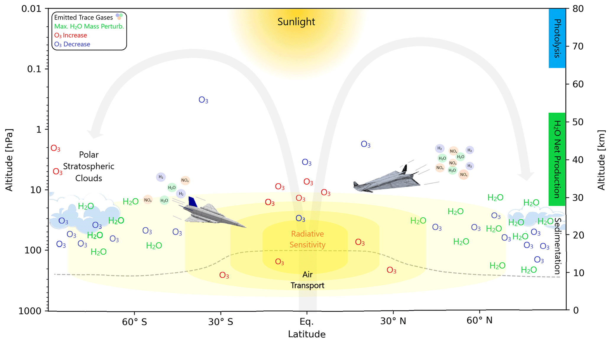
Figure 10 Overview of the average atmospheric sensitivities of water vapor and ozone to hypersonic emissions of water vapor, nitrogen oxides, and hydrogen and the most important atmospheric processes. Shown in yellow is the approximate radiative sensitivity to trace gas changes.

Atmospheric perturbations were calculated with the full-scale atmospheric chemistry and general circulation model EMAC, and the perturbations were fed to a radiation model to calculate the stratospheric-adjusted radiative forcing. Additionally, the study includes an evaluation of EMAC H₂O and O₃ mixing ratios. Briefly summarized, the model excels in modeling O₃ and underestimates H₂O mixing ratios in the middle atmosphere. The model setup was based on a novel approach to reduce the cost of computation and effectively reduced the simulated years by one-third.

The method to calculate changes in atmospheric composition and associated stratospheric-adjusted radiative forcings for different emission regions allows a comparison of their specific sensitivities. The main results are condensed in two quick-look tables of atmospheric and radiative sensitivities (Tables 4, 5), visualized in Fig. 10, and other results are mostly for explanation and analysis. The main message is that differences in sensitivities can be manifold depending on the latitude and altitude of emission. The most important large-scale process controlling the lifetime of perturbations certainly is the Brewer–Dobson circulation. But also, local processes like polar stratospheric cloud chemistry can contribute strongly depending on emission location. From the calculated sensitivities, H₂O emission and the related H₂O perturbation, in addition to NO_x emission, which causes O₃ perturbation, have the largest warming potential. Both share the regional pattern (except NO_x emission at 38 km) that emission at low latitudes is associated with the largest radiative sensitivities. However, their altitude sensitivities are (mostly) inverse; i.e., warming from H₂O perturbation increases with altitude, while warming from O₃ changes decreases with altitude at 30–38 km. It might appear in Fig. 10 that regions of the largest water vapor changes in mid-latitudes and polar regions do not overlap very much with the regions of the largest radiative sensitivities in the tropics. However, the overlap clearly suffices to cause significant values of stratospheric-adjusted radiative forcing. The calculated sensitivities allow inexpensive and fast estimates of the stratospheric-adjusted radiative forcing of new hypersonic aircraft designs depending on latitude, altitude, and ratio of emissions without the need to apply a complex atmospheric chemistry general circulation model.

Generally, the results are in line with prior publications (Kinnison et al., 2020; Pletzer et al., 2022), and the altitude optimization potential has already been highlighted by Kinnison et al. (2020) for atmospheric composition changes and by Pletzer et al. (2022) for atmospheric composition changes and radiation. An additional highlight is an extension of the H₂O perturbation lifetime in the literature to higher levels (Fig. 8). Further work may include the analysis of HS-sens model results with respect to the seasonal sensitivity that may enhance the mitigation potential when adapting aircraft trajectories to the seasonal changes in circulation and chemistry.

Appendix A

A1 Methods and simulations

A1.1 EMAC model setup HS-sens

​​​​​​​In the HS-sens model setup we used the following submodels for physics: AEROPT (Aerosol OPTical properties), CLOUD, CLOUDOPT (CLOUD OPTical properties), CONVECT (CONVECTion), CVTRANS (ConVective Tracer TRANSport), E5VDIFF (ECHAM5 Vertical DIFFusion), GWAVE (Gravity WAVE), OROGW (OROgraphic Gravity Wave), QBO (Quasi Biannual Oscillation), and RAD (RADiation).

AEROPT calculates aerosol optical properties, and CLOUDOPT calculates cloud optical properties (Dietmüller et al., 2016). CLOUD accounts for cloud cover, cloud micro-physics, and precipitation and is based on the original ECHAM5 subroutines, as is CONVECT, which calculates convection processes (Roeckner et al., 2006). CVTRANS is directly linked and calculates the transport of tracers due to convection. E5VDIFF addresses vertical diffusion and land–atmosphere exchanges, excluding tracers. GWAVE and OROGW account for (non-)orographic gravity waves. QBO includes winds of observed quasi-biannual oscillations. RAD and RAD_FUBRAD contain the extended ECHAM5 radiation scheme and allow multiple radiation calls like stratospheric adjusted radiative forcing (Dietmüller et al., 2016).

For chemistry, we used the following submodels: AIRSEA, CH4, DDEP (Dry DEPosition), H2OEMIS (H₂O EMISsion), JVAL (J Values), LNOX (Lightning Nitrogen OXides), MECCA (Module Efficiently Calculating the Chemistry of the Atmosphere), MSBM (Multiphase Stratospheric Box Model), OFFEMIS (OFFline EMISsion), ONEMIS (ONline EMISsion), SCAV (SCAVenging), SEDI (SEDImentation), SURFACE and TNUDGE (Tracer NUDG(E)ing), and TREXP (Tracer Release EXPeriments).

AIRSEA calculates the deposition and emission over the ocean, which corrects the global budget of tracers like methanol and acetone (Pozzer et al., 2006). CH4 determines the oxidation of methane (CH₄) by the hydroxyl radical OH, atomic oxygen O(¹D), chlorine, and photolysis (Winterstein and Jöckel, 2021). In the HS-sens setup the feedback to specific humidity is activated in MECCA. DDEP accounts for the dry deposition of aerosol tracers and gas phase tracers, and SEDI accounts for the sedimentation of aerosols and their components (Kerkweg et al., 2006). H2OEMIS adds H₂O emissions to specific humidity via TENDENCY (Pletzer et al., 2022). JVAL calculates the photolysis rate coefficients (Sander et al., 2014). LNOX contributes a parametrization (Grewe) for NO_x production by lightning for intra-clouds and clouds to the ground (Grewe et al., 2001; Tost et al., 2007). MECCA accounts for all internal tracers related to the production and destruction of chemical components (Sander et al., 2005, 2011). MSBM calculates the polar stratospheric cloud chemistry and is based on the PSC (Polar Stratospheric Cloud) submodel code (Jöckel et al., 2010). The representation of polar stratospheric clouds includes three subtypes of polar stratospheric clouds, i.e., solid nitric acid trihydrate (NAT) particles (type 1a), super-cooled ternary solutions (HNO₃, H₂SO₄, H₂O; type 1b), and solid ice particles (type 2) (Kirner et al., 2011). The latter start to form below the frost point. Multiple parameters regarding polar stratospheric clouds are written as output within EMAC. Examples are mixing ratios of relevant trace gases (HNO₃, HCl, HBr, HOCl, HOBr) in liquid, solid, or gas phase; number densities of ice and NAT particles; and loss and production of NAT through sedimentation. Further included are the physical parameters of the velocity, radius, and surface of particles. OFFEMIS prescribes emission data like relative concentration pathways (RCPs), and ONEMIS calculates emissions online; both are added to internal-tracer tendencies (Kerkweg et al., 2006). SCAV accounts for wet deposition and liquid-phase chemistry in precipitation fluxes (Tost et al., 2006). SURFACE originates from several ECHAM5 subroutines and calculates temperatures of different surfaces (Roeckner et al., 2006). TNUDGE is responsible for tracer nudging (Kerkweg et al., 2006).

Additional diagnostics were activated via the following submodels: CONTRAIL, DRADON (Decay RADioactive ONline), O3ORIG (O₃ ORIGin), ORBIT, PTRAC (Passive TRACer), SATSIMS (Satellites Simulator), SCALC (Simple CALCulations), TBUDGET (Tracer BUDGET), TENDENCY, S4D (Sampling in 4 Dimensions), SCOUT (Stationary Column OUTput), SORBIT (Satellite ORBIT), TROPOP (TROPOsPhere) and VISO (Vertically layered ISO – surfaces and maps). We mainly used PTRAC for verification of emitted trace gases, TENDENCY to account for and verify the specific humidity budget, and TROPOP for the global WMO tropopause height during post-analysis.

A1.2 Evaluation with satellite data

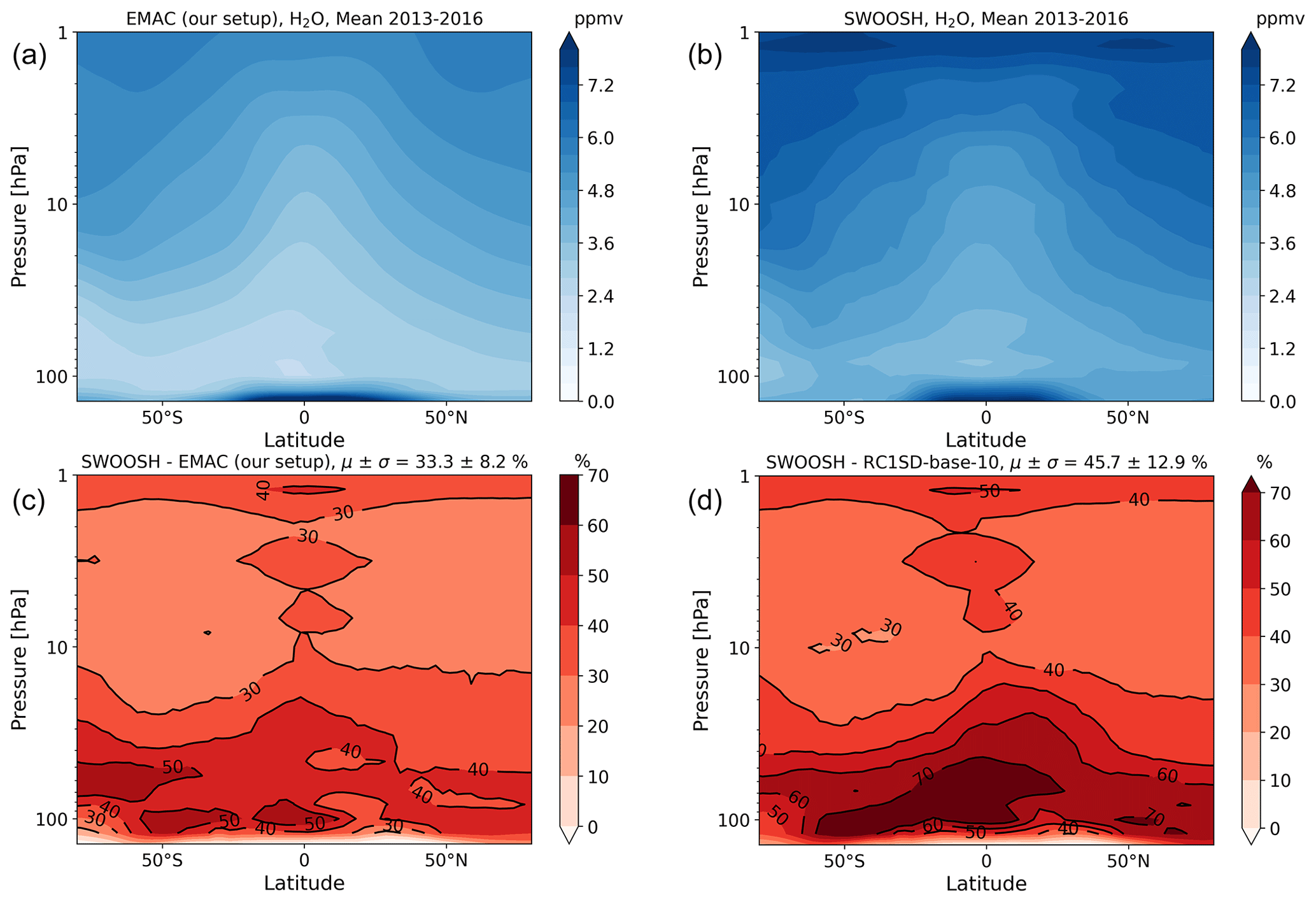
Figure A1 Multi-annual mean of water vapor volume mixing ratio for the EMAC setup used in this work (a), SWOOSH multi-instrumental mean satellite data (b), and the difference (observation–model) in percent for our model setup (c) and RC1SD-base-10 (d).

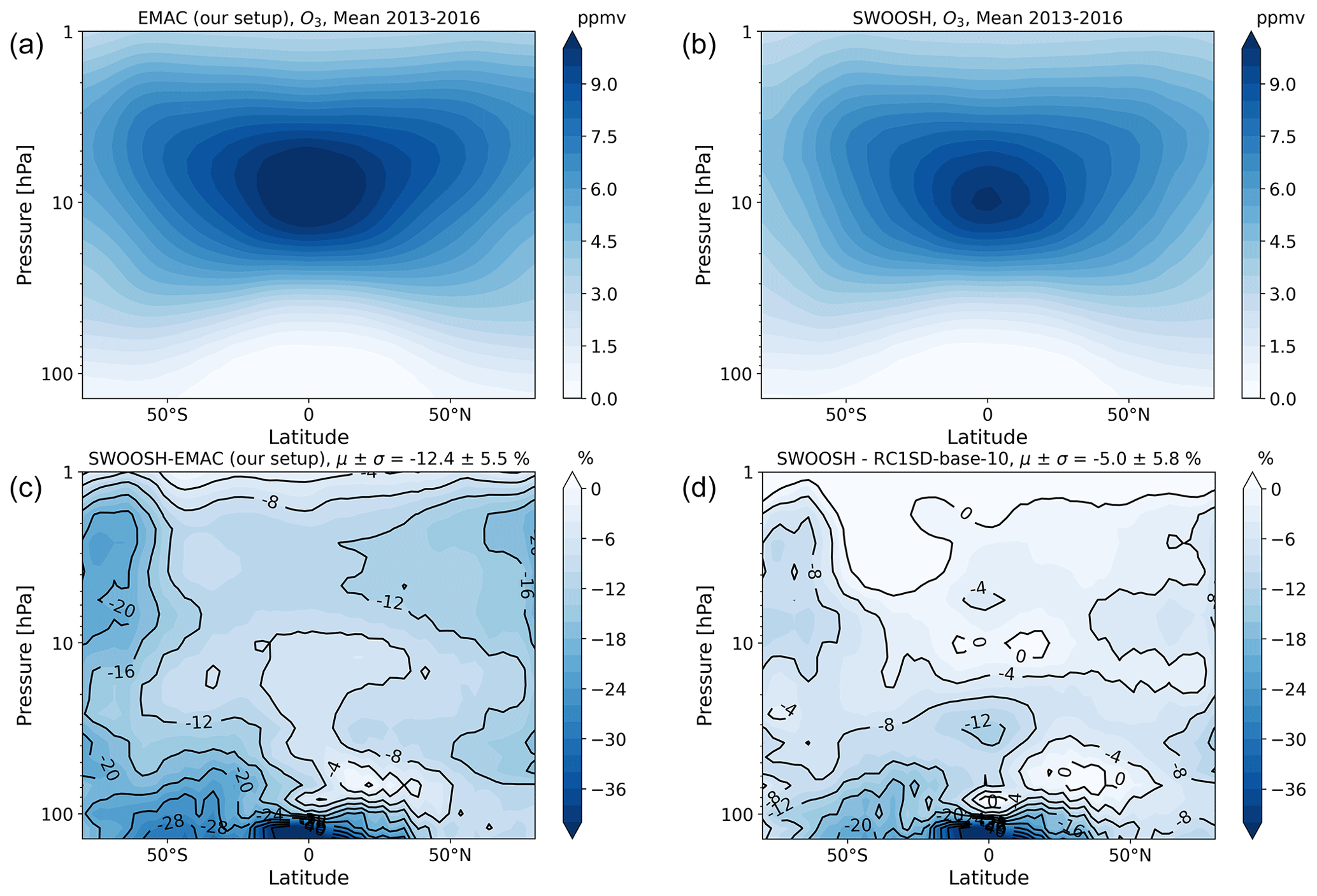
Figure A2 Multi-annual mean of ozone volume mixing ratio for the EMAC setup used in this work (a), SWOOSH multi-instrumental mean satellite data (b), and the difference (observation-model) in percent for our model setup (c) and RC1SD-base-10 (d).

A1.3 Enhancing the efficient use of computing resources

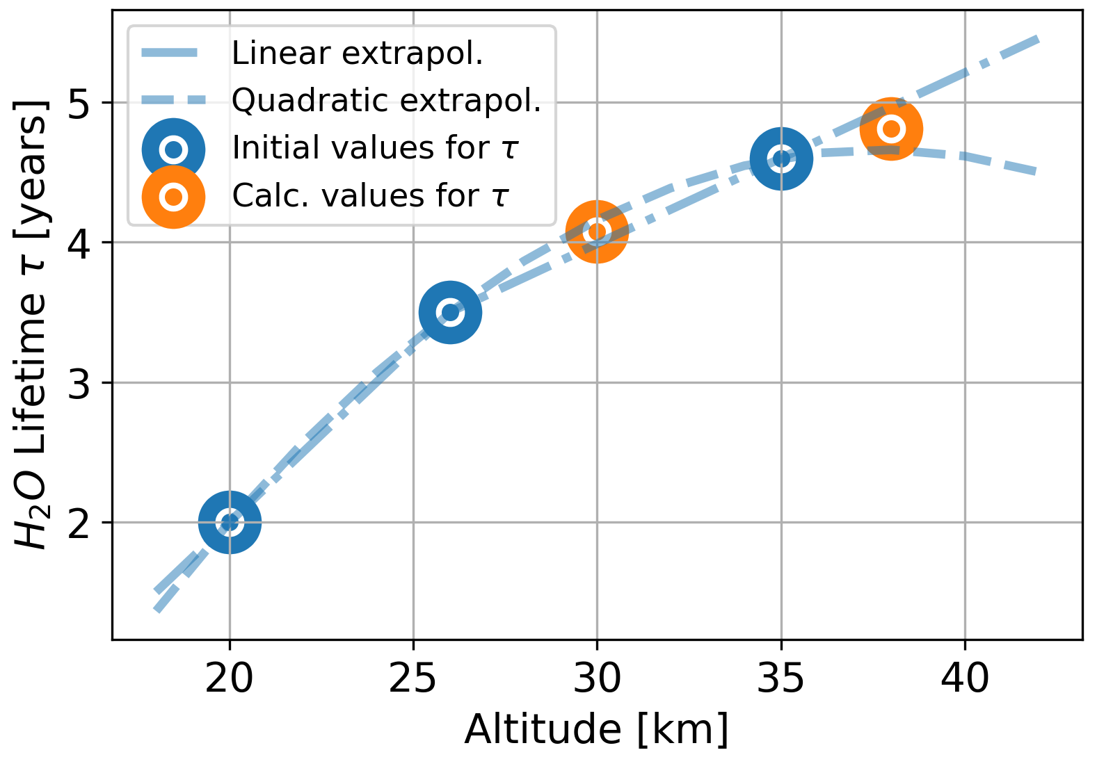
Figure A3 Water vapor perturbation lifetime τ depending on altitude. Blue circles represent initial data that were used for interpolation and extrapolation of orange data circles. Dashed and dashed-dotted blue lines show the behavior of quadratic and linear interpolation and extrapolation, respectively. Orange data circles are based on the average of linear and quadratic interpolation and extrapolation. The values of the orange circles were used to calculate s with Eq. (6).

A2 Emission scenarios

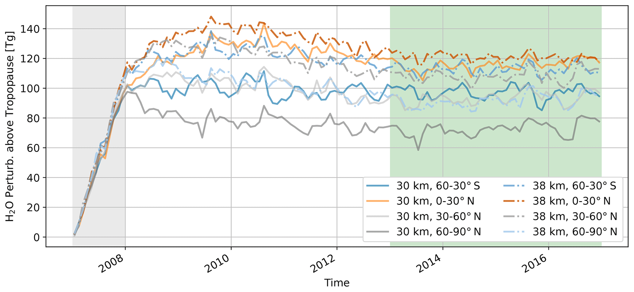
Figure A4 Timeline of monthly mean water vapor perturbation in teragram for scenarios where water vapor is emitted. The first year (gray-shaded area) shows the enhanced emission by the factor s, i.e., the speed-up; 2013–2016 (green-shaded area) shows the years in multi-annual mean equilibrium. The white- and gray-shaded areas (2007–2012) mark the spin-up phase.

A3 Atmospheric composition changes

A3.1 Methane lifetime

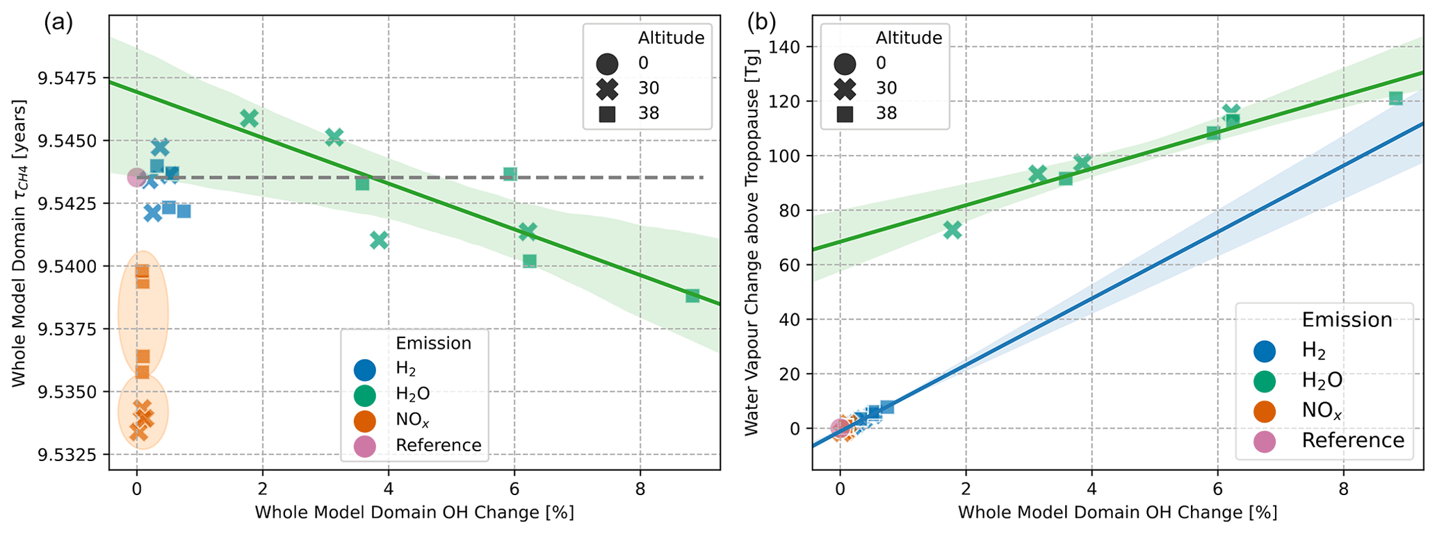
Figure A5 Methane lifetime (whole model domain) is shown in (a) and the water vapor mass perturbation (b) in relation to the relative hydroxyl radical mass change (whole model domain) for all emission scenarios (legend). Whole-model-domain methane lifetime is reduced or extended below or above the dashed gray line, respectively. The regression lines including the shaded areas depict the mean and standard deviation of scenarios.

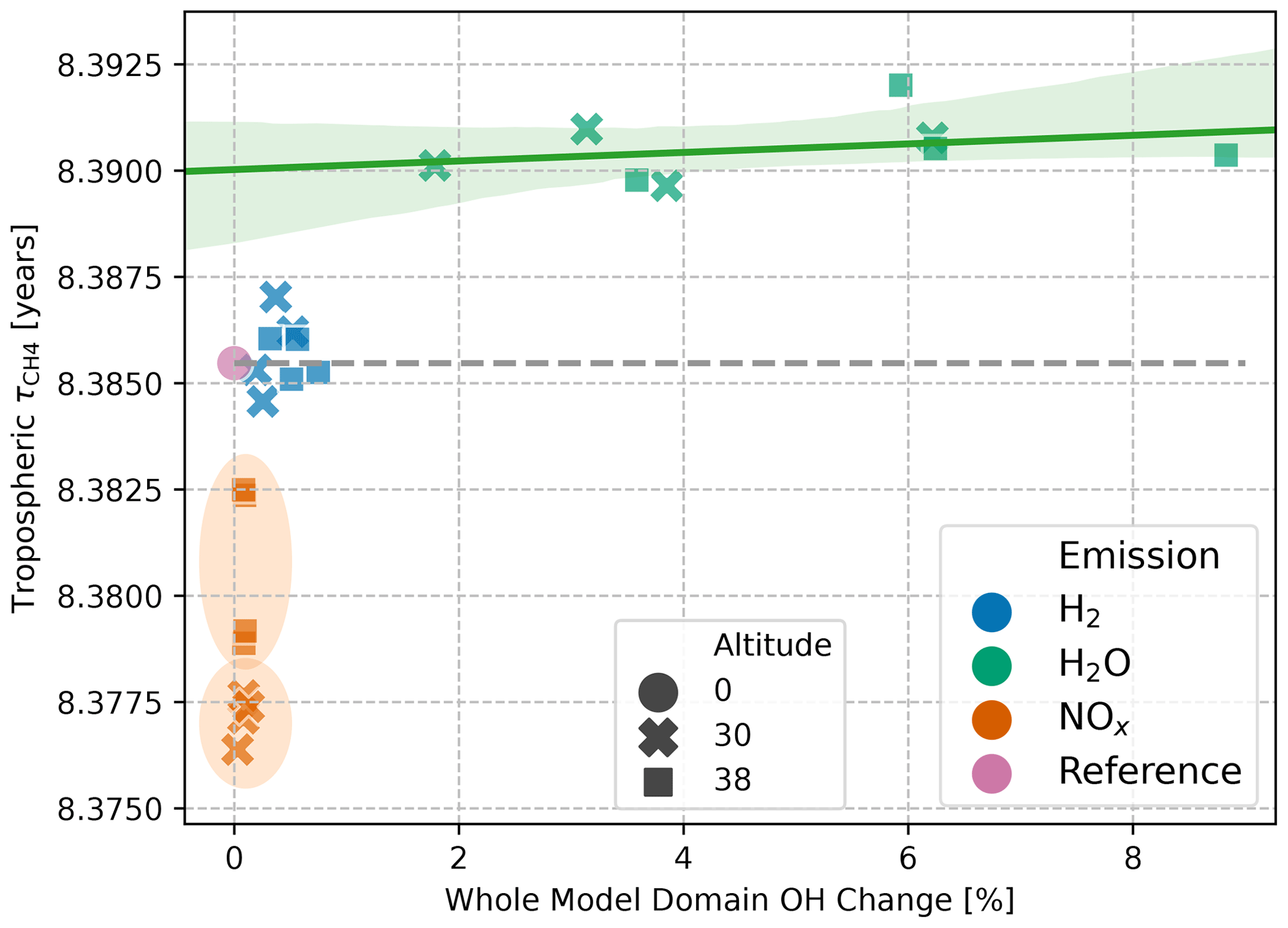
Figure A6 Tropospheric methane lifetime in relation to hydroxyl change (whole model domain) for all emission scenarios (legend). Tropospheric methane lifetime is reduced or extended below or above the dashed gray line, respectively. The regression lines including the shaded areas depict the standard deviation of scenarios.

A3.2 Water vapor emission

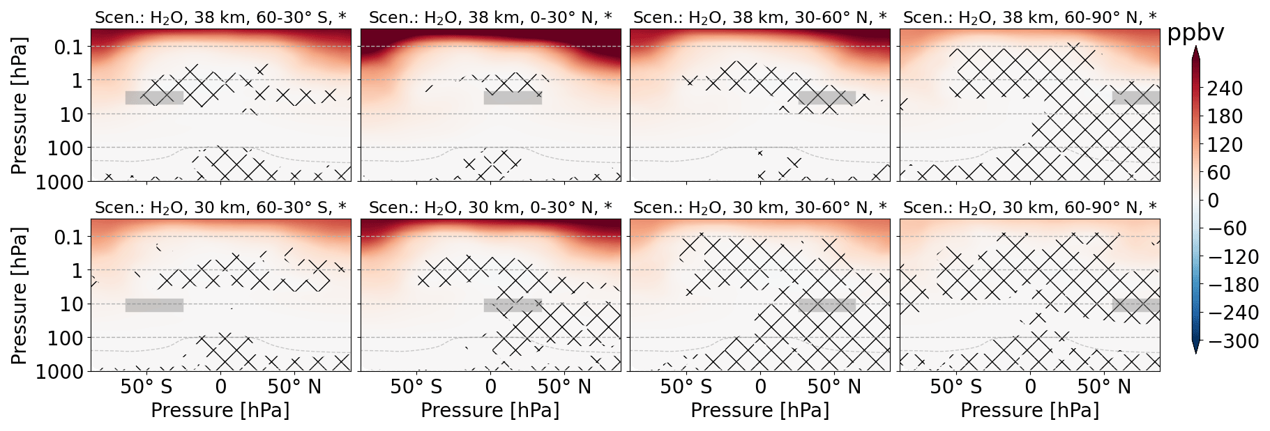
Figure A7 Zonal mean of H₂ perturbation (volume mixing ratio, ppbv) for scenarios where H₂O is emitted. The first and second rows refer to 38 and 30 km altitudes of emission, respectively. Columns represent the latitude region of emission. The emission regions are shaded in gray. Lines indicate statistically insignificant results, and the probability level is written in the title of each subplot.

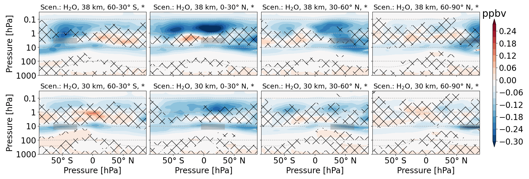
Figure A8 Zonal mean of NO_x perturbation (volume mixing ratio, ppbv) for scenarios where H₂O is emitted. The first and second rows refer to 38 and 30 km altitudes of emission, respectively. Columns represent the latitude region of emission. The emission regions are shaded in gray. Lines indicate statistically insignificant results, and the probability level is written in the title of each subplot.

A3.3 Nitrogen oxide emission and ozone perturbation

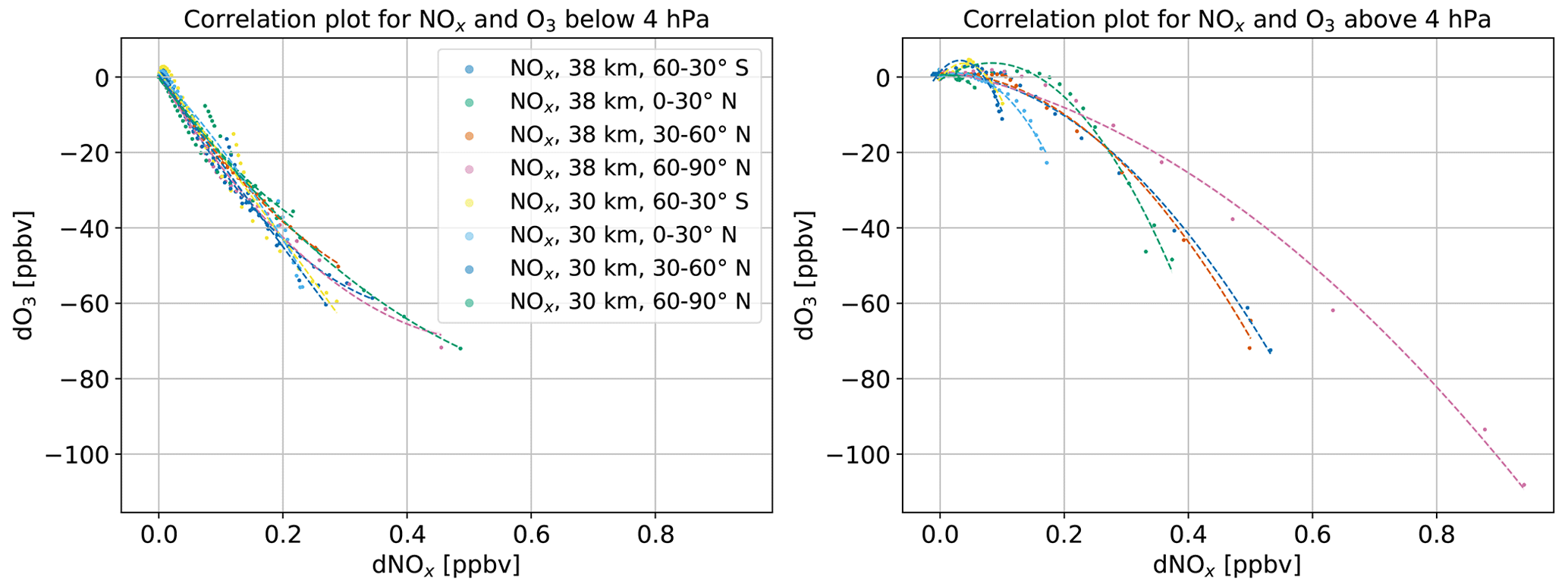
Figure A9 Correlation of nitrogen oxide change and ozone change for two altitudes regions (surface–4 and 4–0.01 hPa). The values are averaged over latitude and limited to statistically significant values with a 95 % confidence.

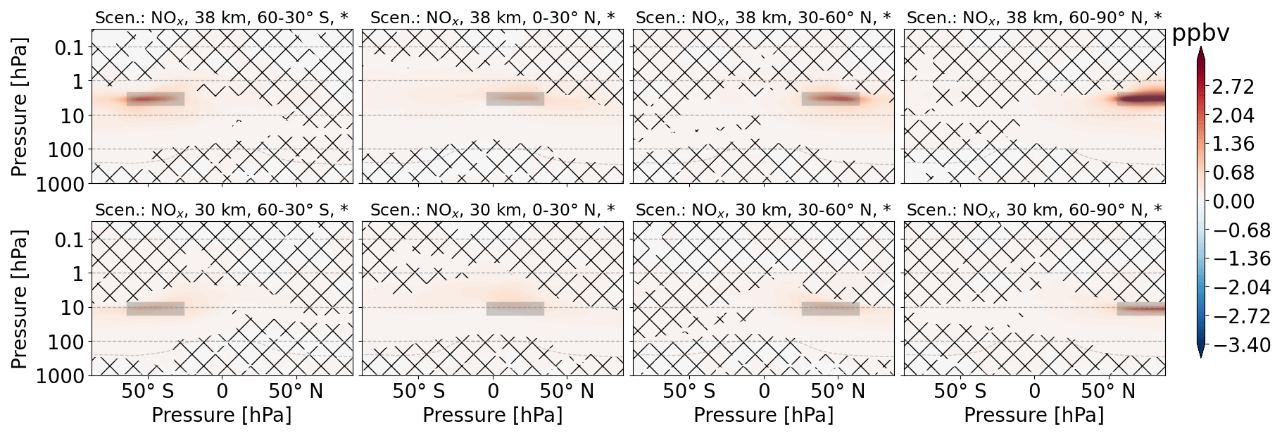
Figure A10 Zonal mean of NO_x perturbation (volume mixing ratio, ppbv) for scenarios where NO_x is emitted. The first and second rows refer to 38 and 30 km altitudes of emission, respectively. Columns represent the latitude region of emission. The emission regions are shaded in gray. Lines indicate statistically insignificant results, and the probability level is written in the title of each subplot.

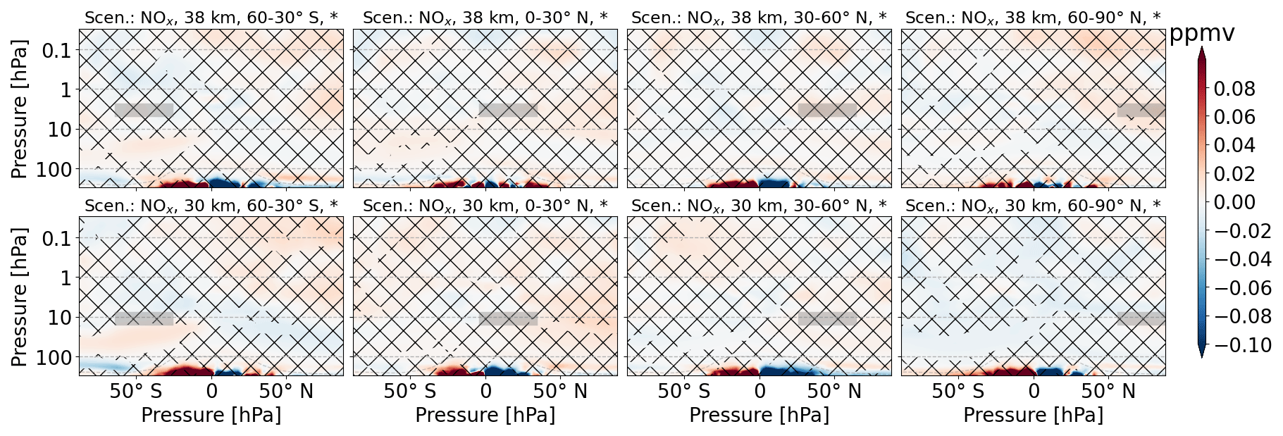
Figure A11 Zonal mean of H₂O perturbation (volume mixing ratio, ppbv) for scenarios where NO_x is emitted. The first and second rows refer to 38 and 30 km altitudes of emission, respectively. Columns represent the latitude region of emission. The emission regions are shaded in gray. Lines indicate statistically insignificant results, and the probability level is written in the title of each subplot.

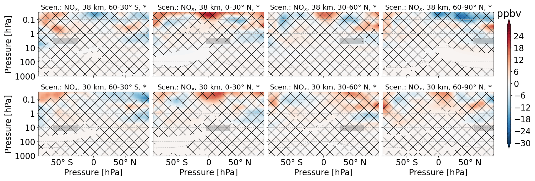
Figure A12 Zonal mean of H₂ perturbation (volume mixing ratio, ppbv) for scenarios where NO_x is emitted. The first and second rows refer to 38 and 30 km altitudes of emission, respectively. Columns represent the latitude region of emission. The emission regions are shaded in gray. Lines indicate statistically insignificant results, and the probability level is written in the title of each subplot.

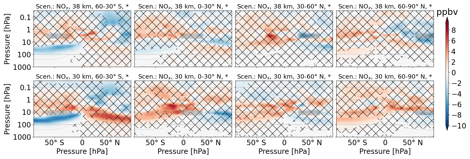
Figure A13 Zonal mean of CH₄ perturbation (volume mixing ratio, ppbv) for scenarios where NO_x is emitted. The first and second rows refer to 38 and 30 km altitudes of emission, respectively. Columns represent the latitude region of emission. The emission regions are shaded in gray. Lines indicate statistically insignificant results, and the probability level is written in the title of each subplot.

A3.4 Hydrogen emission

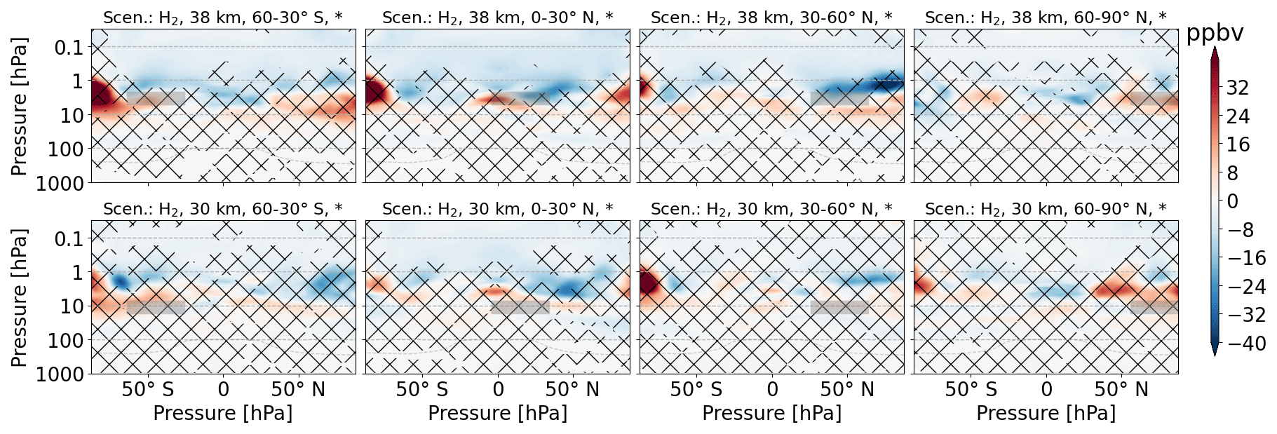
Figure A14 Zonal mean of O₃ perturbation (volume mixing ratio, ppbv) for scenarios where H₂ is emitted. The first and second rows refer to 38 and 30 km altitudes of emission, respectively. Columns represent the latitude region of emission. The emission regions are shaded in gray. Lines indicate statistically insignificant results, and the probability level is written in the title of each subplot.

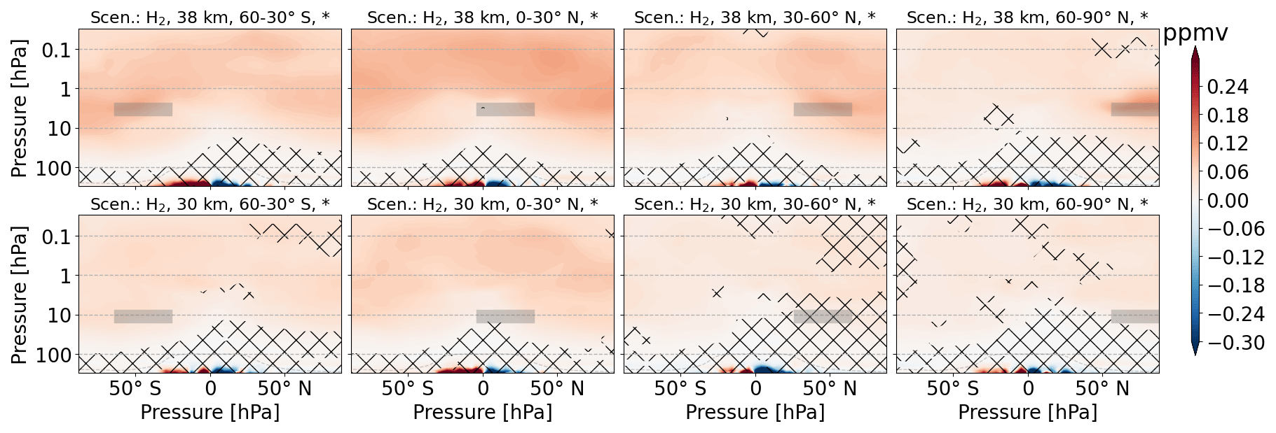
Figure A15 Zonal mean of H₂O perturbation (volume mixing ratio, ppmv) for scenarios where H₂ is emitted. The first and second rows refer to 38 and 30 km altitudes of emission, respectively. Columns represent the latitude region of emission. The emission regions are shaded in gray. Lines indicate statistically insignificant results, and the probability level is written in the title of each subplot.

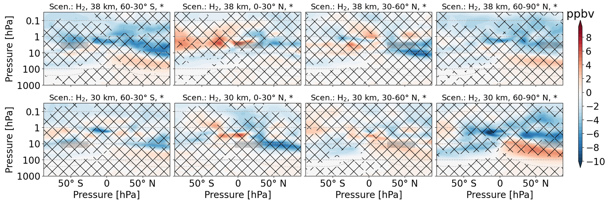
Figure A16 Zonal mean of CH₄ perturbation (volume mixing ratio, ppbv) for scenarios where H₂ is emitted. The first and second rows refer to 38 and 30 km altitudes of emission, respectively. Columns represent the latitude region of emission. The emission regions are shaded in gray. Lines indicate statistically insignificant results, and the probability level is written in the title of each subplot.

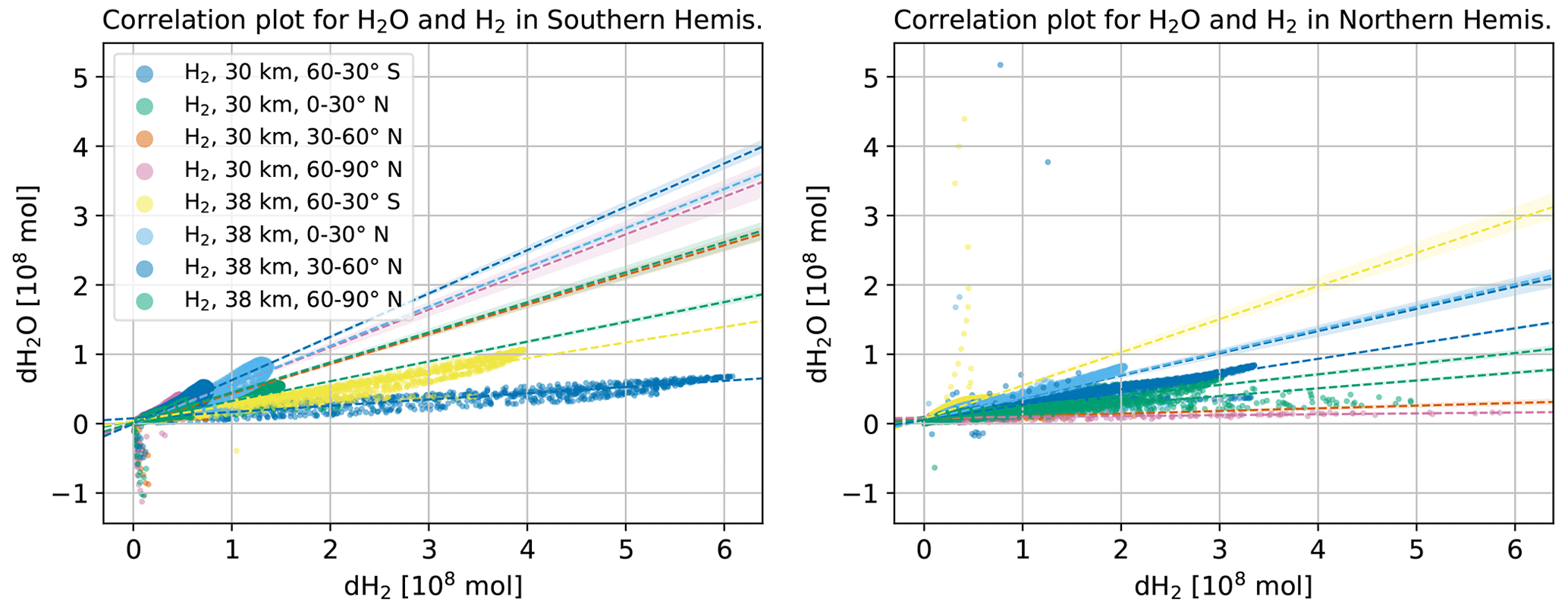
Figure A17 Correlation of molar water vapor and hydrogen change for the Southern (a) and Northern (b) Hemisphere. The values are limited to statistically significant values with a 95 % confidence.

A3.5 Overview on atmospheric composition

Table A1 Average atmospheric composition changes per molecule of emitted species.

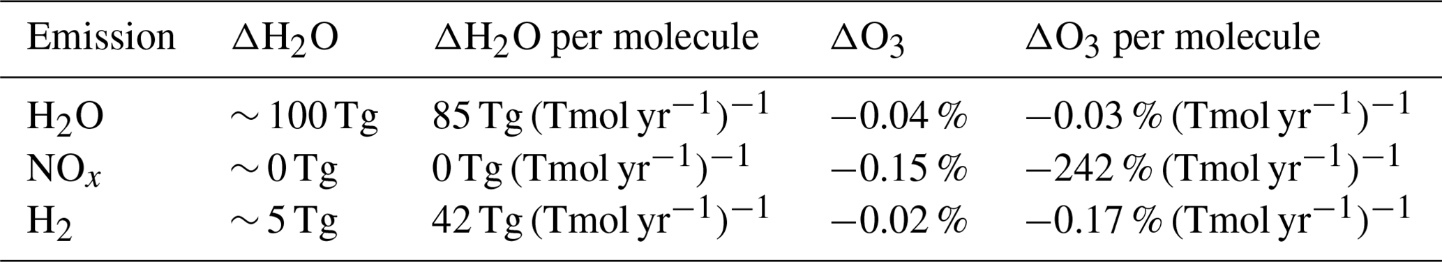
Table A2 Relative atmospheric composition change of CH₄, HO₂, and OH (average) for the troposphere and middle atmosphere.

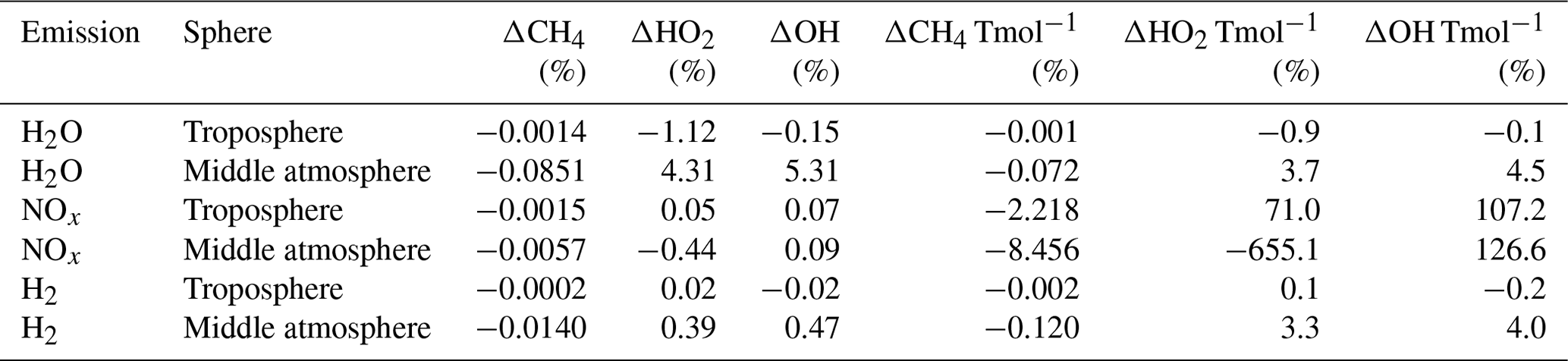
A4 Radiative forcing

A4.1 Water vapor radiative forcing

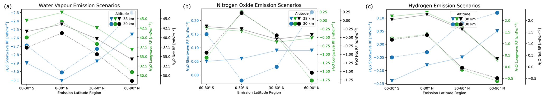
Figure A18 The shortwave, longwave, and net radiative forcing in blue, green, and black, respectively, for water vapor (a), nitrogen oxide (b), and hydrogen (c) emission scenarios due to water vapor changes. For different altitude emission scenarios, refer to markers. Latitude regions of emission are aligned on the x axis.

A4.2 Ozone radiative forcing

Figure A19 The shortwave, longwave, and net radiative forcing in blue, green, and black, respectively, for water vapor (a), nitrogen oxide (b), and hydrogen (c) emission scenarios due to ozone changes. For different altitude emission scenarios, refer to markers. Latitude regions of emission are aligned on the x axis.

A4.3 Methane radiative forcing

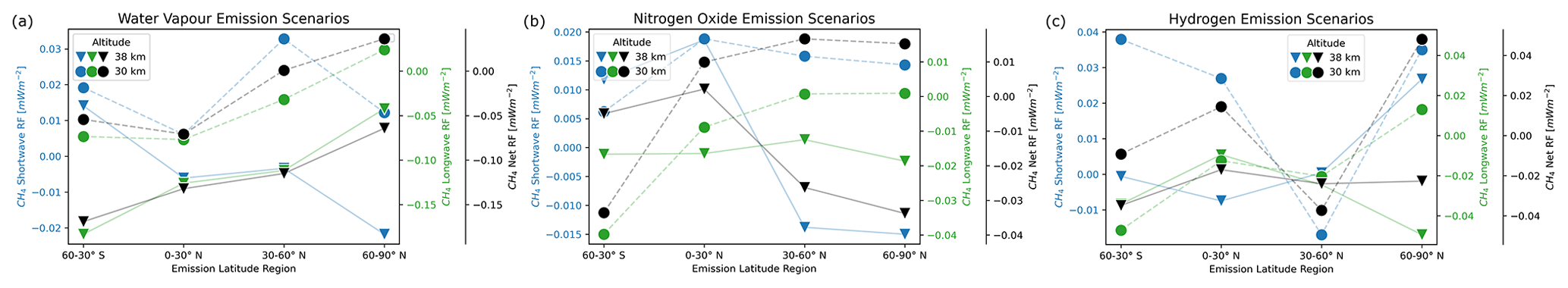
Figure A20 The shortwave, longwave, and net radiative forcing in blue, green, and black, respectively, for water vapor (a), nitrogen oxide (b), and hydrogen (c) emission scenarios due to methane changes. For different altitude emission scenarios, refer to markers. Latitude regions of emission are aligned on the x axis.

A4.4 Individual radiative forcing and the related perturbations

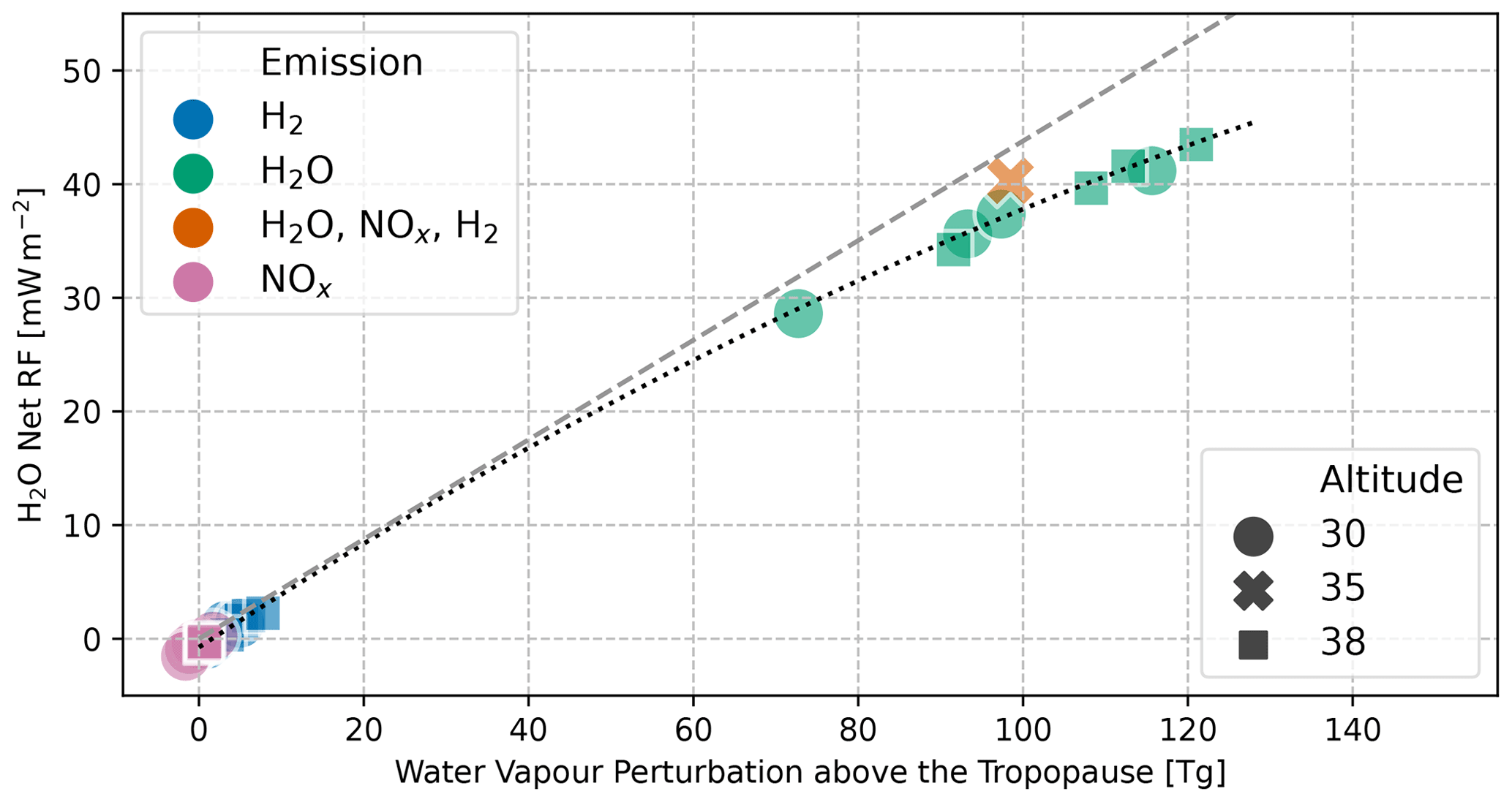
Figure A21 Overview of H₂O net radiative forcing for all 24 simulations. Colors refer to the initial emission (H₂, H₂O, and NO_x), and markers refer to the altitude of emission. The green cross for 35 km altitude refers to the publication of Pletzer et al. (2022) and is based on a global emission scenario (aircraft LAPCAT MR2) where H₂, H₂O, and NO_x are emitted simultaneously. The gray line refers to a correlation of RF and H₂O perturbation from another publication (Fig. 8 in Grewe et al., 2014a). The dotted black line is a two-dimensional polynomial fit with $a{x}^{\mathrm{2}}+bx+c$, where a = −0.88, b = 473.73 and c = −746.76 W m⁻² Tg⁻¹.

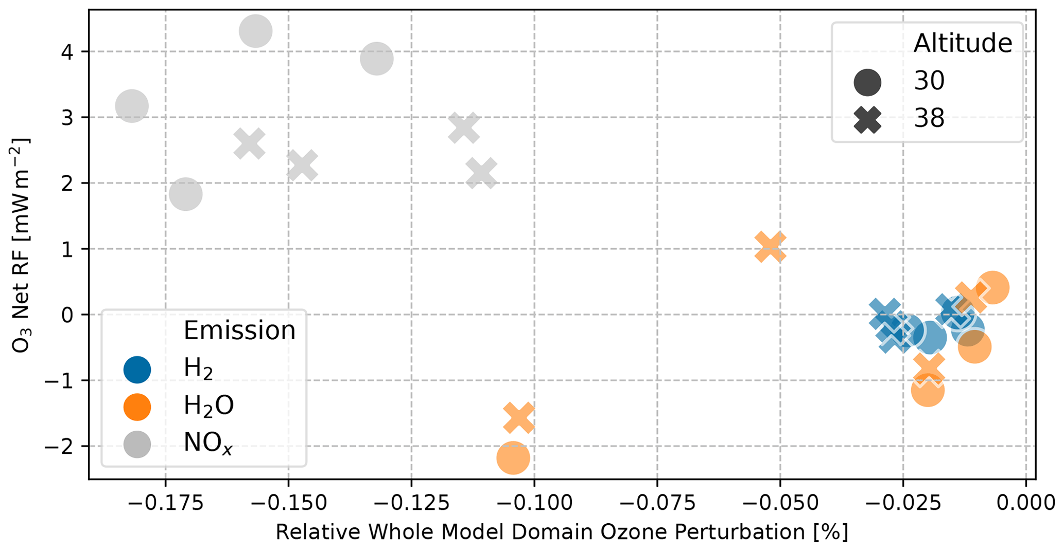
Figure A22 Overview of O₃ net radiative forcing for all 24 simulations. Colors refer to the initial emission (H₂, H₂O, and NO_x), and markers refer to the altitude of emission.

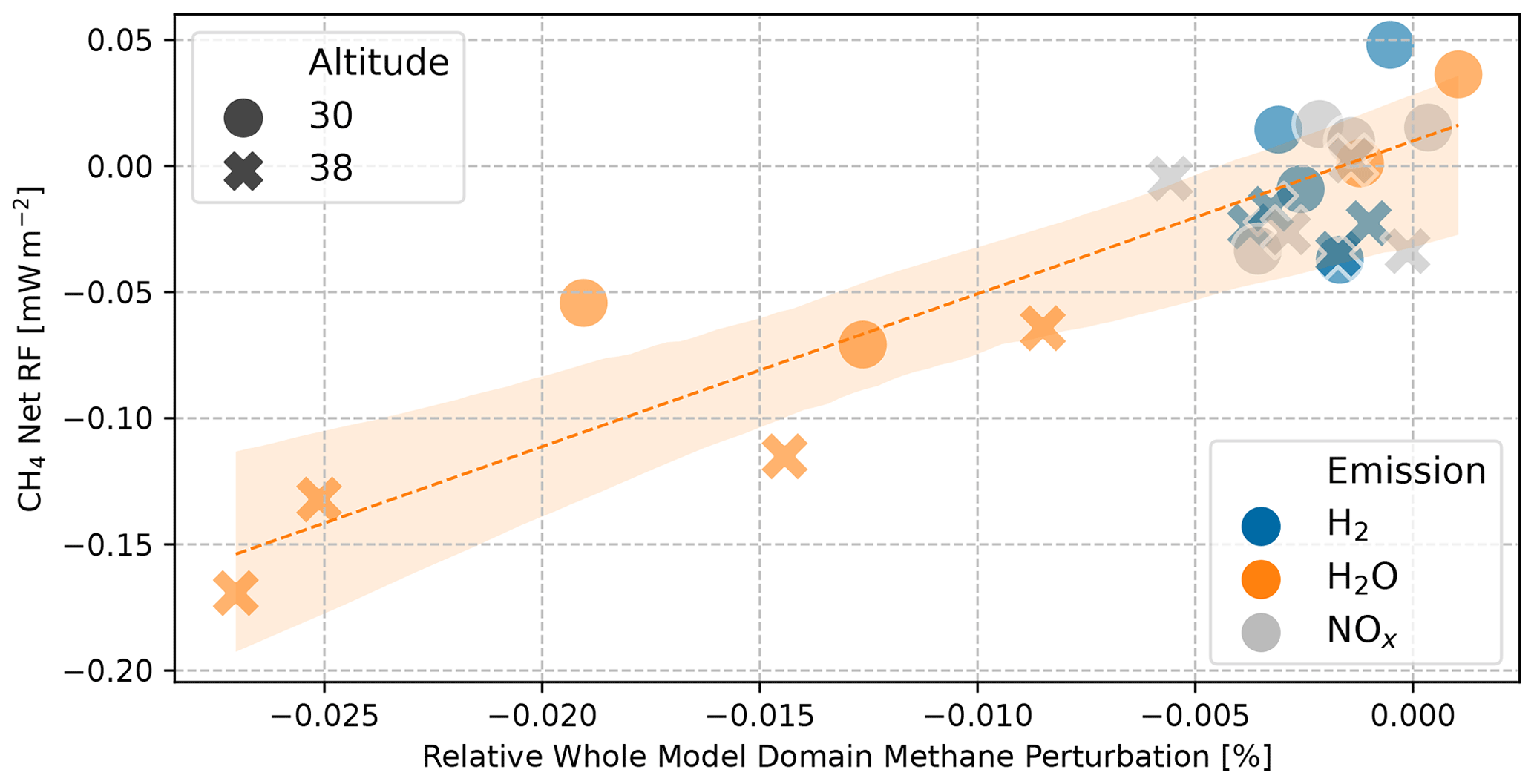
Figure A23 Overview of CH₄ net radiative forcing for all 24 simulations. Colors refer to the initial emission (H₂, H₂O, and NO_x), and markers refer to the altitude of emission. The regression line, including the shaded areas, depicts the mean and standard deviation of the eight H₂O emission scenarios.

A5 Discussion of atmospheric composition changes and radiative forcing

A5.1 Water vapor atmospheric and radiative sensitivities

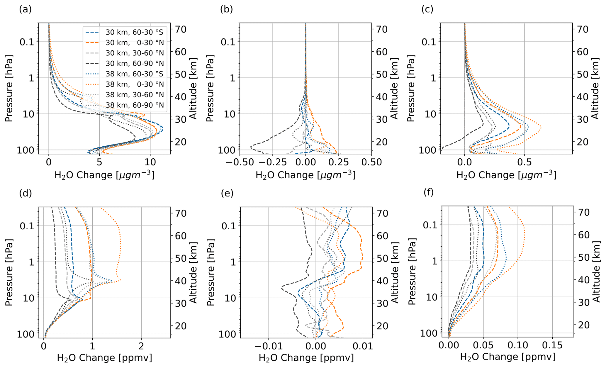
Figure A24 Vertical distribution of global H₂O change as concentration (a, b, c) and volume mixing ratio (d, e, f). Panels (a) and (d), (b) and (e), and (c) and (f) depict H₂O change due to H₂O, NO_x, and H₂ emission, respectively.

A5.2 Ozone atmospheric and radiative sensitivities

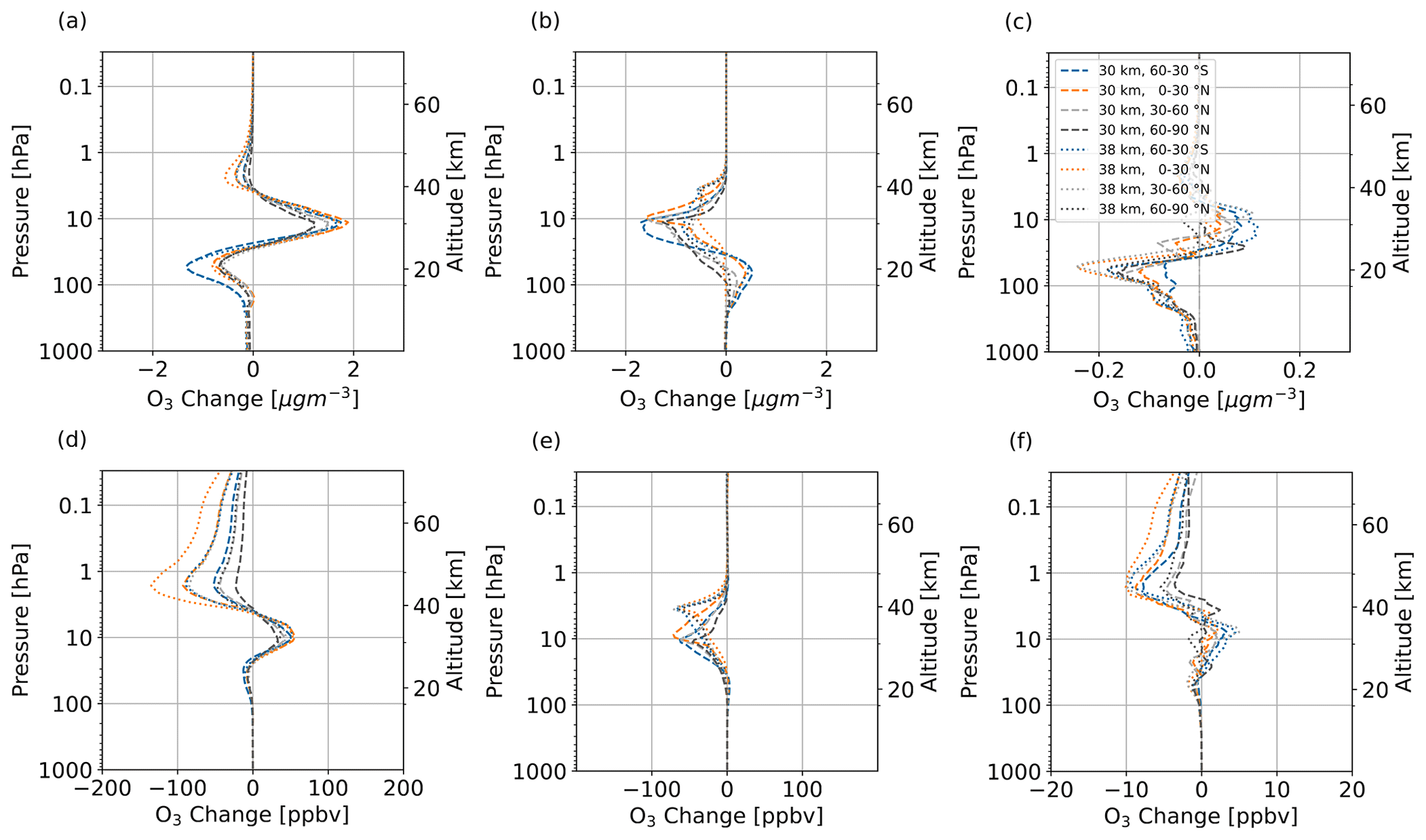
Figure A25 Vertical distribution of global O₃ change as concentration (a, b, c) and volume mixing ratio (d, e, f). Panels (a) and (d), (b) and (e), and (c) and (f) depict O₃ change due to H₂O, NO_x, and H₂ emission, respectively.

A6 Conclusion and discussion

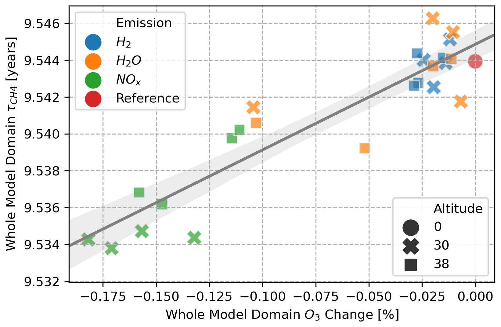
Figure A26 Methane lifetime in relation to ozone change (both whole model domain) for all emission scenarios (legend). The gray regression line, including the shaded area, depicts the 95 % confidence interval of all scenarios.