Dynamical linear modeling estimates of long-term ozone trends from homogenized Dobson Umkehr profiles at Arosa/Davos, Switzerland

Six collocated spectrophotometers based in Arosa/Davos, Switzerland, have been measuring ozone profiles continuously since 1956 for the oldest Dobson instrument and since 2005 for the Brewer instruments. The datasets of these two ground-based triads (three Dobsons and three Brewers) allow for continuous intercomparisons and derivation of long-term trend estimates. Mainly, two periods in the post-2000 Dobson D051 dataset show anomalies when compared to the Brewer triad time series: in 2011–2013, an offset has been attributed to technical interventions during the renewal of the spectrophotometer acquisition system, and in 2018, an offset with respect to the Brewer triad has been detected following an instrumental change on the spectrophotometer wedge.

In this study, the worldwide longest Umkehr dataset (1956–2020) is carefully homogenized using collocated and simultaneous Dobson and Brewer measurements. A recently published report (Garane et al., 2022) described results of an independent homogenization of the same dataset performed by comparison to the Modern-Era Retrospective analysis for Research and Applications version 2 (MERRA-2) Global Modeling Initiative (M2GMI) model simulations. In this paper, the two versions of homogenized Dobson D051 records are intercompared to analyze residual differences found during the correction periods. The Aura Microwave Limb Sounder (MLS) station overpass record (2005–2020) is used as an independent reference for the comparisons. The two homogenized data records show common correction periods, except for the 2017–2018 period, and the corrections are similar in magnitude.

In addition, the post-2000 ozone profile trends are estimated from the two homogenized Dobson D051 time series by dynamical linear modeling (DLM), and results are compared with the DLM trends derived from the collocated Brewer Umkehr time series. By first investigating the long-term Dobson ozone record for trends using the well-established multilinear regression (MLR) method, we find that the trends obtained by both MLR and DLM techniques are similar within their uncertainty ranges in the upper and middle stratosphere but that the trend's significances differ in the lower stratosphere. Post-2000 DLM trend estimates show a positive trend of 0.2 to 0.5 % yr⁻¹ above 35 km, significant for Dobson D051 but lower and therefore nonsignificantly different from zero at the 95 % level of confidence for Brewer B040. As shown for the Dobson D051 data record, the trend only seems to become significantly positive in 2004. Moreover, a persistent negative trend is estimated in the middle stratosphere between 25 and 30 km. In the lower stratosphere, the trend is negative at 20 km, with different levels of significance depending on the period and on the dataset.

1 Introduction

The stratospheric ozone layer is essential for its role in protecting the Earth's surface from harmful solar ultraviolet radiation. Stratospheric ozone depletion occurring during the second half of the twentieth century has been contained by the strict application of the Montreal Protocol and its amendments (MontrealProtocol, 1987). While in the upper stratosphere (10–1 hPa, 32–48 km), ozone has started to show significant signs of recovery (e.g. Petropavlovskikh et al., 2019), in the lower stratosphere (147–32 hPa, 13–24 km), measurements show that ozone is still decreasing (Ball et al., 2018). Uncertainties remain for the middle stratospheric trends (32–10 hPa, 24–32 km), with different composites showing different changes, giving a picture of a relatively flat trend with low significance (Ball et al., 2018).

Intensive discussions about the significance of the lower stratospheric trends and about the discrepancies between the magnitudes of the model simulated and the measured ozone trends are ongoing in the recent literature. Chipperfield et al. (2018) point to large interannual variability rather than an ongoing downward trend. Wargan et al. (2018) confirm the negative trend in the lower stratosphere in the Northern Hemisphere (NH) using dynamical linear modeling (DLM) on the Modern-Era Retrospective analysis for Research and Applications version 2 (MERRA-2) reanalysis. Sensitivity analyses by Ball et al. (2019) and Dietmüller et al. (2021) support the negative NH lower stratosphere trends highlighting, for the former, the overestimated magnitude of the final-year (–2018) anomalies by the models and, for the latter, the underestimated probability density function of the model trends as causes for the bad accordance between the simulated and measured ozone lower stratospheric trends. Orbe et al. (2020) associate the negative NH lower stratospheric trends with a change in advection, describing a northward upwelling expansion associated with an enhancement of the downwelling over NH midlatitudes. In this case, the discrepancies in magnitude between the lower stratospheric trends retrieved from the measurements and from the model (MERRA-2 Global Modeling Initiative (M2GMI) reanalysis) are attributed to an imperfect simulation of the tropical convective processes and of the 2016 inversion of the quasi-biennial oscillation (QBO).

Multilinear regression (MLR) is widely and consistently used for vertically resolved ozone trend estimation. This is the dominant method in the recent and past trend estimates literature (e.g., Petropavlovskikh et al., 2019; Sofieva et al., 2021; Maillard Barras et al., 2020; McPeters et al., 1996b; Reinsel et al., 2002; Tummon et al., 2015; WMO, 1998; Staehelin et al., 2001, and references therein). Trend estimates are obtained by fitting a MLR function to the monthly mean ozone time series, presuming a linear dependence of the ozone content towards the explanatory variables and a linear increase or decrease of the ozone content over time. Upper stratospheric post-2000 ozone trends are reported to be significantly positive in the three broad latitude bands, with values of ∼ 2.2 ± 0.7 % per decade at 2.1 hPa in the NH, while nonsignificant negative ozone trends are derived in the lowermost stratosphere, with however large uncertainties (Godin-Beekmann et al., 2022).

The sensitivity of the post-2000 trend magnitude to the start and end years has been extensively discussed (e.g., Petropavlovskikh et al., 2019; Bernet et al., 2019; Dietmüller et al., 2021). Nonmonotonic post-2000 trends are also reported in Arosio et al. (2019), where MLR trends are estimated from a merged SCIAMACHY (SCanning Imaging Absorption spectroMeter for Atmospheric CHartographY), OMPS (Ozone Mapping and Profiler Suite) and SAGE (Stratospheric Aerosol and Gas Experiment) II dataset for the 2003 to 2018 period. In their study, stratospheric tropical trends are shown to be negative during the 2004 to 2011 period and positive from 2012.

Trend estimates by DLM are recent in the literature. First reports are from Laine et al. (2014), who developed the DLM analysis for trend evaluation and applied it to a merge of SAGE II and GOMOS (Global Ozone Monitoring by Occultation of Stars) data records. They compare trend estimates by DLM to trend estimates by piecewise MLR, the latter being described in a companion paper by Kyrölä et al. (2013). They conclude that DLM is a robust method well suited for modeling ozone time series changes (see Sect. 4.2). Their results show a statistically significant turnaround in the ozone time series after 1997 at midlatitudes in the 35 to 55 km altitude range and a more complex behavior of the ozone concentration than the description which can be made by a simple piecewise multilinear regression model. Consequently, stronger ozone variations (decrease or increase) are reported locally when estimated by DLM than by MLR. Ball et al. (2017) applied DLM on a Bayesian composite (BASIC – BAyeSian Integrated and Consolidated) of satellite data records. The changes in ozone between 1998 and 2012 estimated using DLM indicate a clear and significant ozone recovery in the upper stratosphere. DLM has also been used to estimate trends in the lower stratosphere based on the merged SWOOSH/GOZCARDS (Stratospheric Water and Ozone Satellite Homogenized/Global OZone Chemistry And Related Datasets for the Stratosphere) data records (Ball et al., 2018) as discussed previously. More recently, DLM trend estimates on SOS (SAGE II, Osiris (Optical Spectrograph and InfraRed Imaging System) and SAGE III) merged satellite data record are reported (Bognar et al., 2022) and indicate a clear upper stratospheric ozone recovery with varying turnaround years depending on the latitude, a decrease since 2012 in the NH upper/middle stratosphere, but without excluding a step in the Osiris dataset as a cause, and a persistent decrease in the tropical lower stratosphere.

Dobson Umkehr ozone profile data records, which are distributed all around the world (Petropavlovskikh et al., 2022; Godin-Beekmann et al., 2022; Stone et al., 2015; Miyagawa et al., 2009; Garane et al., 2022), have been extensively used in the pre-1998 stratospheric trend estimates (Reinsel et al., 1989; Randel et al., 1999; Miller et al., 1995). Beginning in 1956 for the oldest, the Umkehr records were unique at that time since satellites records only became available in 1979 (McPeters et al., 1996a; Bhartia et al., 2013), and ozonesondes, starting in 1960 (Smit et al., 2007), do not reach the upper stratosphere. Few studies based exclusively on Umkehr measurements report on NH post-2000 stratospheric ozone trends (Zanis et al., 2006; Park et al., 2013). Zanis et al. (2006) derived trends from the Arosa Dobson Umkehr dataset and reported statistically significant negative trends in the 1970 to 1995 period and the first signs of a reversing trend in the lower and the upper stratosphere for the period 1996 to 2004. Since this turnaround was not statistically significant, the authors suggested that the dataset should be reevaluated at a future stage when more measurements become available. The homogenized Umkehr time series was used by Park et al. (2013) to derive trends using functional mixed models and in the frame of the LOTUS project (Petropavlovskikh et al., 2019), which derived stratospheric ozone trends from improved and combined datasets (satellites, ground-based instruments and models). The NH trends derived from the Umkehr datasets are in accordance with trends derived from other ground-based instruments for the pre-1997 period and the post-2000 period. Umkehr data also corroborate the satellite findings, showing highly statistically significant evidence of declining ozone concentrations since the mid-1980s in the upper stratosphere and post-2000 positive trends ranging between 2.0 % and 3.1 % per decade in the upper stratosphere of NH midlatitudes. The Umkehr data records are still extensively used for trend estimates along with datasets from other ground-based techniques, satellites and models (Steinbrecht et al., 2017; Harris et al., 2015; Petropavlovskikh et al., 2019; Tarasick et al., 2019; Godin-Beekmann et al., 2022). However, trend estimations on Brewer Umkehr data records are sparse. A study using simple linear regression, without consideration of explanatory variables, applied to data from the Brewer 005 of Thessaloniki presented by Fragkos et al. (2018) reports 1997–2017 statistically significant positive trends, in the NH, above 35 km of 0.3 % yr⁻¹ and nonstatistically significant trends below. Fitzka et al. (2004) report on linear trends estimated with the Sen's Q method and significances assessed with the Mann–Kendall test. We innovate here by estimating Brewer Umkehr trends considering explanatory variables in the regression by DLM.

The dataset quality is of primary importance for trend studies, and multi-instrument comparison analyses are suited to assess the long-term stability of data records by estimating the drift and bias of instruments (Hubert et al., 2016). Using microwave radiometer data records, Bernet et al. (2019) showed the effect of instrumental artifacts on the long-term ozone profile trends. Recently, trends estimated on updated and reprocessed ozone profiles datasets have resulted in reduced trend uncertainties (Godin-Beekmann et al., 2022).

The quality of the Arosa/Davos total column ozone (TCO) dataset is currently under investigation by a reprocessing and a homogenization with the use of the ozone absorption cross section from Serdyuchenko et al. (2014) (Gröbner et al., 2021) and the consideration of the effects of the relocation from Arosa to Davos (Stübi et al., 2021b). In Arosa/Davos, the Dobson D051 is the station's primary instrument for continuous Umkehr profile time series. It was dedicated exclusively to Umkehr measurement from 1988 until February 2013, when total ozone measurement was added to the schedule. The number of observations dedicated to Umkehr was not impacted, and the number of retrieved Dobson D051 Umkehr profiles was kept to two profiles per day up to now. This frequency in observations allows for the computation of statistically reliable monthly means for trend estimations. However, the instrument operations recently suffered from anomalies following technical interventions. Therefore, a complete homogenization of the Dobson D051 Umkehr data record has been performed and is described in this paper. Trend estimations free from known instrumental artifacts can then be derived from this dataset.

The paper is organized as follows: the data sources used in this study are described in Sect. 2, with a special focus on the Umkehr method description. In Sect. 3, the complete homogenization of the Dobson D051 Umkehr data record is detailed and compared to the homogenization performed by NOAA on the same data record in the frame of the ESA project WP-2190 (Garane et al., 2022). The MLR and DLM trend estimate methods are described in Sect. 4, with a comparison of the trend values resulting from both regressions on the same Dobson D051 data record. Results of vertically resolved long-term trend estimates by DLM are presented and discussed in Sect. 5, followed by conclusions in Sect. 6.

2 Data sources

2.1 Umkehr data records from Arosa/Davos

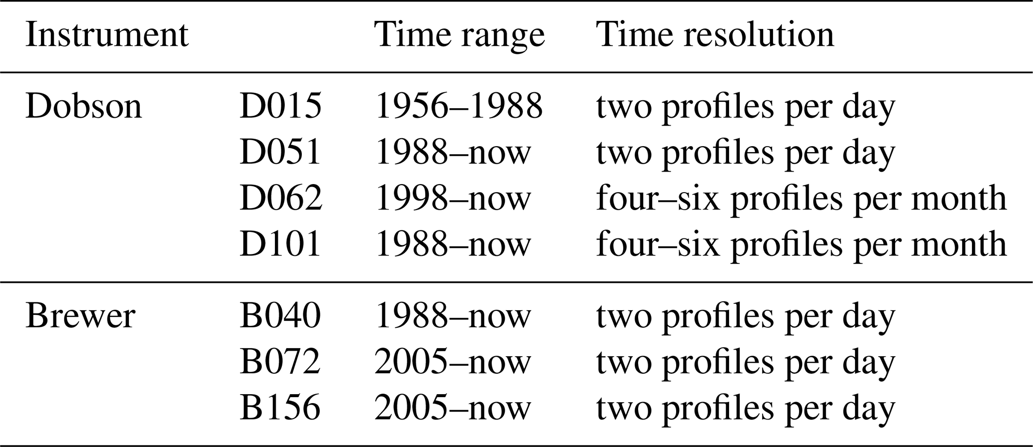
The Umkehr technique, which will be described in Sect. 2.1.1, allows for the low-resolution retrieval of ozone profiles from measurements made by Dobson and Brewer spectrophotometers. TCO and ozone profile measurements with Dobson (and Brewer) spectrophotometers were performed at Arosa (46.82^∘ N, 6.95^∘ E) from 1926 (and 1988) to 2021 and at Davos from 2012. For a detailed description of the Dobson and Brewer spectrophotometers, we refer to Stübi et al. (2021a, 2017a). The progressive relocation of the Dobson and Brewer triads from Arosa to Davos (13 km north of Arosa and 260 m lower in altitude) between 2012 and 2021 is described and analyzed in Stübi et al. (2017b, 2021b). Umkehr measurements have been performed under clear-sky and low cloud cover conditions twice a day since 1956 by Dobson spectrophotometers (Dobson D015 since 1956 and then Dobson D051 since 1988) and four to six times per month by Dobson D101 since 1988 and by Dobson D062 since 1998. Dobson D051 performs fully automated Umkehr measurements since 1988. The Dobson Umkehr measurements have been complemented by Brewer Umkehr measurements since 1988 with Brewer B040 and since 2005 with Brewers B072 and B156. See Table 1 for a summary of the time ranges and time resolutions of the six Arosa/Davos spectrophotometers. Ozone profile Umkehr measurements were initiated in 1956 at Arosa and were continued from 2021 at Davos, Switzerland. They compose the longest continuous Umkehr measurement time series worldwide (Staehelin et al., 2018).

Table 1 Time ranges and time resolutions of the Dobson and Brewer Umkehr measurements at the Arosa/Davos station.

At Arosa, the Dobson D051 sat on a turntable in a conditioned hut maintained at 25–28 ^∘C. An aperture in the roof, which opened and closed according to solar zenith angle (SZA) and weather conditions, allowed for zenith measurements. The continuous and automated measurements (2 min cycle) are interpolated to 12 nominal SZAs, and profiles are retrieved from the ground to 50 km using the optimal estimation method (OEM) (Rodgers, 2000) implemented in Petropavlovskikh et al. (2005a). Manual Umkehr measurement started in 1968 with the Dobson D101 and in 1992 with the Dobson D062 as redundant measurements to check the stability of Dobson D051. These have been made two to three times each month since 1988 and 1998 in favorable weather conditions. The Dobson D062 and the Dobson D101 were automated in 2012 and in 2013, respectively (Stübi et al., 2021b). They have been located since 2021 in Davos in a common air-conditioned container side by side with the Dobson D051 and measure Umkehr curves through a quartz dome. While the Dobson D051 was dedicated exclusively to Umkehr measurement until February 2013, the present setup allows for both direct sun and zenith Umkehr measurements with the three Dobsons. The Arosa/Davos Dobson instruments are regularly calibrated against the two European regional secondary reference Dobson instruments D064 from the Hohenpeissenberg Observatory (MOHp, Germany) and D074 from the Solar and Ozone Observatory in Hradec Králové (SOO-HK, Czech Republic) (Stübi et al., 2021b, Fig. 3).

The Brewer triad consists of two Brewer Mark II single-monochromator instruments, the Brewer B040 and the Brewer B072, and one Brewer Mark III double-monochromator instrument, the Brewer B156. The three instruments measure daily in Umkehr mode when the sun is at the 12 nominal SZAs. Since the operation of the first Brewer at Arosa in 1988, biennial calibrations have been carried out (Stübi et al., 2017a, Fig. 1) towards the traveling reference instrument Brewer B017 and, since 2008, towards the traveling reference instrument Brewer B185. The instruments of the Brewer triad underwent very few technical interventions and are in good agreement with the traveling references (TCO deviations ≤ 1 %; Stübi et al., 2017a). In particular, no technical issues are reported around 2011–2013 and 2018, which are data record periods considered in the frame of the Dobson D051 homogenization. However, sporadic instabilities in the Brewer B072 data record have been observed, while no particular technical issues have been detected by the intercomparison procedures. The Dobson D051, the Brewer B072 and the Brewer B156 were simultaneously relocalized from Arosa to Davos in September 2018 but with an effect on the TCO level within the instrumental noise (Stübi et al., 2017a, 2021b).

2.1.1 The Umkehr method

The Umkehr method is based on the measurement of the ratio of downward scattered zenith sky radiation for two wavelengths in the UVB–UVA range from 300 to 330 nm (Huggins absorption band) which are subject to different strengths of ozone absorption, the shorter wavelength being more strongly absorbed by ozone. This ratio changes as a function of SZA during sunset and sunrise due to changes in the scattering height along the zenith (Mateer, 1965; Stone et al., 2015). As the SZA increases from 60 to 90^∘, the scattering height increases, and the two intensities decrease because of increased absorption and scattering by ozone and air molecules. As the shorter wavelength has a higher scattering point than the longer wavelength, its intensity decreases faster than the longer wavelength intensity as long as both scattering heights are below the ozone maximum. At high SZA, the scattering height for the shorter wavelength is above the ozone maximum, and the scattering height of the longer wavelength is still below the ozone maximum. The shorter wavelength intensity decreases then less rapidly than the longer wavelength intensity, and the ratio reaches a maximum at high SZA, called the Umkehr effect (Götz et al., 1934). The Umkehr method allows for the retrieval of ozone profiles from the measurements by Dobson and Brewer spectrophotometers. We describe the particularities of Dobson and Brewer Umkehr measurements in the following subsections.

Figure 1 (a) Morning (in black) and afternoon (in blue) N curves at 12 nominal SZAs and (b) their corresponding retrieved ozone profiles in Dobson units (DU) as a function of altitude in kilometers and pressure level in hectopascals (hPa). Total column ozone and atmospheric conditions slightly differ between the morning and the afternoon. The altitude ranges of the 10 Dobson layers (DLs) are shown in (b). Lower, middle and upper stratospheric ranges are displayed by beige shading.

2.1.2 Umkehr measurements by Dobson spectrophotometers

The logarithm of the ratio of the two wavelength intensities (R values) is converted to radiance using calibration tables (RtoN table) and reported as N values (Fig. 1a) in N units for 12 nominal SZAs between 60 and 90^∘ (60, 65, 70, 74, 77, 80, 83, 85, 86.5, 88, 89 and 90^∘). The nominal wavelength pairs used in a Dobson spectrophotometer are A – 305.5 and 325.4 nm, C – 311.45 and 332.4 nm, and D – 317.6 and 339.8 nm. Two narrow slits separate the respective wavelengths. The ozone profiles (Fig. 1b) are retrieved from the measurements of the C pair intensity, while the total column measurement uses a combination of two wavelength pairs (AD) (Stübi et al., 2021a).

The 12 N values (further called N curve) are screened for clear-sky conditions and corrected for cloud influence using a nearby UV–Vis lux meter. This empirical correction is based on the relation between the UV–Vis intensity of clear days (within the same month, for each SZA) and the UV–Vis intensity variation during the cloudy N curve measurement (see Basher, 1982). This cloud correction is based on a uniform cloud layer and may fail for more complicated cloud structures. Haze correction is not included. It was shown that the effect of small cloud corrections of the N values on the vertically resolved ozone trends is negligible. For these reasons, only profiles retrieved from N curves without any cloud correction or with a small correction are considered for our study.

2.1.3 Umkehr measurements by Brewer spectrophotometers

The intensity of eight wavelengths (306.3, 310.1, 313.5, 316.8, 320.1, 323.2, 326.5 and 329.5 nm) is quasi-simultaneously measured for solar zenith angles changing from 60 and 90^∘. A holographic grating is used as a dispersive element for the solar radiation which then passes through narrow slits centered on the desired wavelengths. Mark II Brewer instruments use one single holographic grating and therefore only one dispersive element to separate the wavelengths. Mark III Brewer instruments are double monochromators that use two holographic gratings (Staehelin et al., 2003). The Umkehr ozone profile can be retrieved from three measured wavelength pairs (McElroy and Kerr, 1995; Stone et al., 2015) by OEM. For similarity with the Dobson Umkehr measurement, the intensity ratio of only two wavelengths is used here: 310.05 nm of short set of wavelengths and 326.5 nm of the long set of wavelengths. The data are flagged for clouds before the interpolation onto the 12 nominal SZAs. The quality filter eliminates data points that fall outside a predefined error envelope determined by the range of natural variability and a mean offset.

2.1.4 Ozone profile retrieval

Retrieved ozone profiles are given on 10 layers between 0 and 50 km with a vertical resolution of 10–15 km. Dobson and Brewer ozone profiles are retrieved by OEM. The Dobson Umkehr retrieval algorithm is described in Petropavlovskikh et al. (2005a), and the Brewer Umkehr retrieval algorithm has been adapted by Petropavlovskikh et al. (2005b) from the Dobson algorithm. The version of the code used in this study has been implemented by Martin Stanek and can be found at http://www.o3soft.eu/o3bumkehr.html (last access: 15 May 2020). Dobson and Brewer Umkehr retrievals use the same a priori profile and ML climatology, described in McPeters and Labow (2012) and formed by combining data from Aura Microwave Limb Sounding (MLS) (2004–2010) with data from ozonesondes (1988–2010). The measurement error covariance matrices are diagonal, with values between 0.16–0.8 N units for Dobson and 0.6–2 N units for Brewer. The Brewer observation errors have been estimated by the standard deviation of the 2005–2018 climatological difference of collocated and simultaneous N value measurements. In the layers below Dobson layer (DL) 4, peaking at 20 km, for both instruments, the averaging kernels (AKs; not shown) show sensitivity of observations to ozone variability in several layers, and therefore the partitioning of the retrieved ozone in individual layers is based on the a priori information.

The quality check of the retrieved ozone profile includes assessment of the number of iterations (fewer than four is considered a good profile) and the condition that the difference between observed and retrieved Umkehr observations at all SZAs remains within measurement uncertainty (Petropavlovskikh et al., 2022).

A generic stray light correction can be applied to reduce systematic biases in the Dobson Umkehr retrieved profiles (Petropavlovskikh et al., 2011). The NOAA version of the Dobson retrieval applies this correction, while the MeteoSwiss (MCH) version does not. The seasonal bias between the Dobson and Brewer ozone records is reduced when a stray light correction is applied to the Dobson record (Petropavlovskikh et al., 2009). Moreover, as a step change in the record can be related to a change in the amount of stray light, a proper correction of the stray light effect can help to reduce the magnitude of the step.

The Dobson D051 Umkehr observations dataset is regularly archived at the World Ozone and Ultraviolet Radiation Data Centre (WOUDC; http://www.woudc.org, last access: 26 October 2022). The Brewers are part of EUBREWNET (http://www.eubrewnet.org/eubrewnet, last access: 30 June 2022), where raw data files are available for registered users.

2.2 Aura MLS

The Microwave Limb Sounder (MLS) is a microwave limb-sounding radiometer on board the Aura Earth-observing satellite, launched in July 2004. Ozone profiles are retrieved from Aura MLS radiance measurements at 240 GHz. Details about the instrument can be found in Waters et al. (2006). Ozone profiles from the version 4.2 dataset are given on 55 pressure levels from 1000 to 1 × 10⁻⁵ hPa (Livesey et al., 2018). However, the useful vertical range for Aura MLS ozone leads us to only consider Aura MLS data from 10 to 75 km (in this range, the Aura MLS vertical resolution is about 2.5–4 km) for Aura MLS overpasses above Arosa (±3^∘ in latitude and ±5^∘ in longitude). These ozone profiles are interpolated on the Umkehr pressure levels p_i and converted to DU following Godson (1962):

$$\begin{array}{}\text{(1)}& X_{\text{DU}}=C\cdot \stackrel{\mathrm{‾}}{X}\cdot (p_i-p_{i-\mathrm{1}}),\end{array}$$

with C = 0.00079 $\mathrm{DU}{\mathrm{hPa}}^{-\mathrm{1}}{\mathrm{ppbv}}^{-\mathrm{1}}$ and $\stackrel{\mathrm{‾}}{X}$ the ozone mean volume mixing ratio (VMR) in parts per billion per volume (ppbv). Approximative heights are given as in Petropavlovskikh et al. (2022).

3 Homogenization of the Dobson D051 dataset

As the quality of a dataset is essential in order to estimate reliable long-term trends with uncertainties as reduced as possible, we first investigate the quality of the Arosa/Davos longest Umkehr ozone profile dataset and proceed to its detailed homogenization.

The worldwide longest Umkehr ozone profile record was recently impacted by short-term anomalies due to instrumental changes and technical issues. It has been homogenized by two simultaneous but independent studies, one by the principal investigator group of the Dobson D051 instrument (further called MCH homogenization) and one by the NOAA (further called NOAA homogenization). Both homogenization processes are described in Sect. 3.1 and 3.2 and compared in Sect. 3.3. Details are provided in this work for the MCH homogenization, while the reader is referred to Garane et al. (2022) and Petropavlovskikh et al. (2022) for details on the NOAA homogenization.

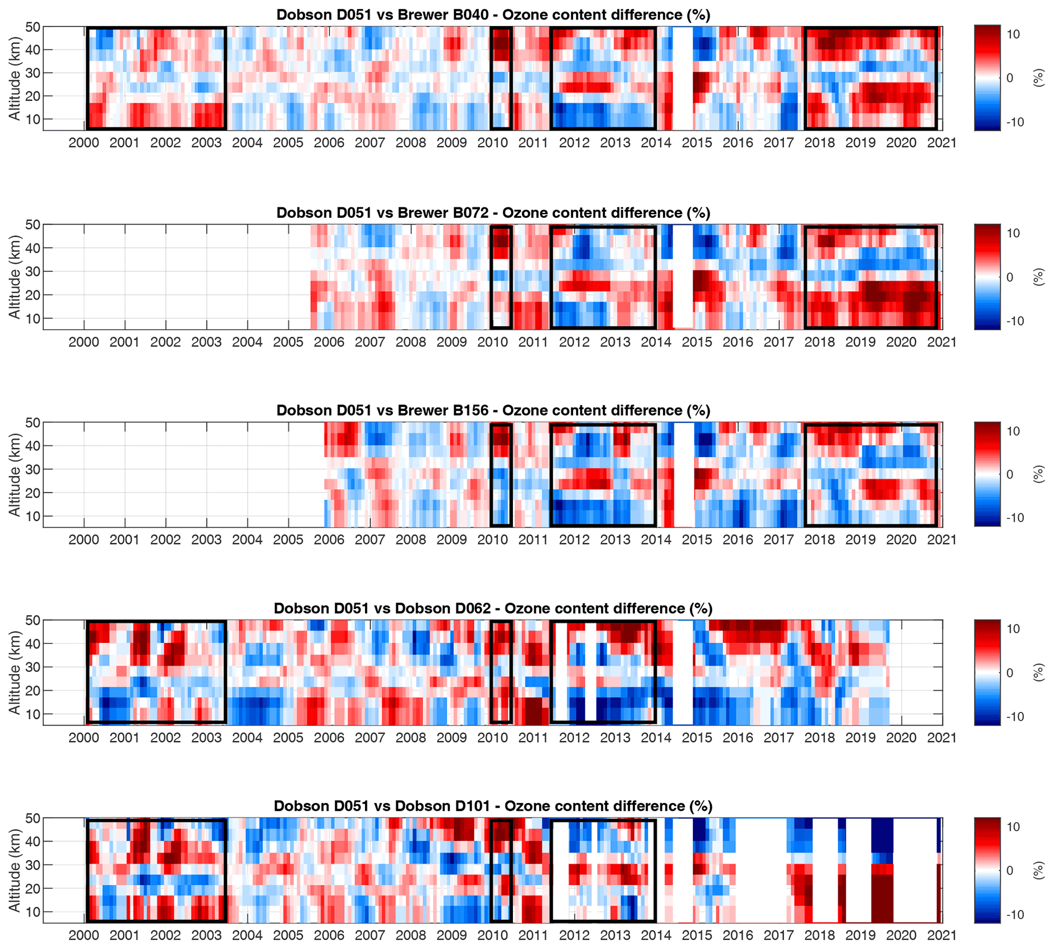
Figure 2 Monthly mean time series of the ozone profiles relative differences for each of the five spectrophotometers with respect to D051. The time series are deseasonalized and smoothed by a 6-month moving average.

3.1 MCH homogenization of the Dobson D051 dataset

The Arosa/Davos Umkehr time series is composed of Dobson D015 measurements from 1956 to 1988 and Dobson D051 since then. The quality of the homogenization of the Dobson D015 to Dobson D051 transition has been ensured by 1 year of parallel measurements (1988), allowing for an adaptation of the D015 N values to the D051 N values. For each SZA, the 1988 mean difference between the D051 and the D015 N values has been added to the D015 values. The 1956–1987 ozone profiles have then been retrieved from the Dobson D015 corrected N values. No statistical correction has been performed on the D015 ozone dataset.

We report here about the complete homogenization of the 1988–2020 Umkehr Dobson D051 time series by comparison to the datasets of the five collocated instruments (two Dobson and three Brewer spectrophotometers) on the N value level. The purpose is to detect common anomalies in the difference between Dobson D051 and each of the redundant measurements and to correct the Dobson D051 time series accordingly. However, a correction is only applied if it correlates with a technical issue reported in the metadata. If we cannot see any indication in the metadata for an instrumental drift, no correction is applied.

Figure 3 Schematic of the Dobson D051 MCH homogenization principle.

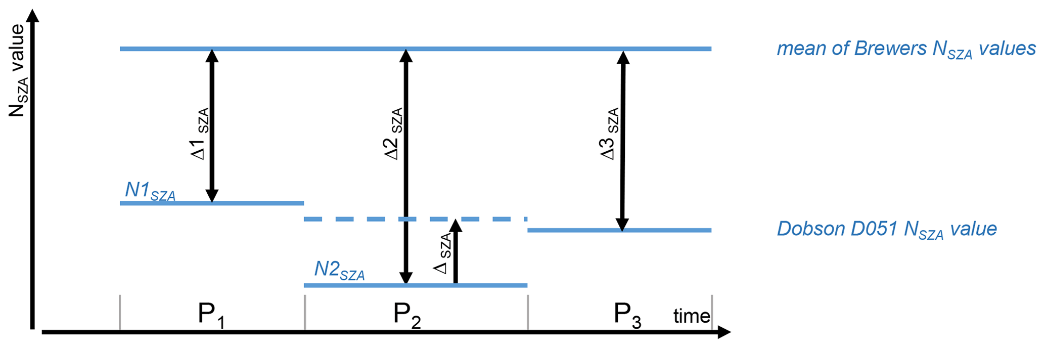
Figure 2 shows the time series of monthly mean ozone profile differences between Dobson D051 and the five collocated spectrophotometers. Only simultaneous measurements, not flagged for bad weather conditions, volcanic eruptions, and number of iterations, are considered. The relative differences of the anomalies lie within ±15 %. The comparisons with the Brewer instruments show a seasonal cycle with differences slightly bigger in summer than in winter (not shown; DL6: −2 % in winter and +2 % in summer). A similar behavior has been found by Gröbner et al. (2021) when comparing TCO from Dobsons to Brewers. Note that the annual cycle is not visible on the representation of deseasonalized anomalies as in Fig. 2 and that we consider changes when they are larger than the standard deviation of the Brewer Dobson differences.

If we focus on the post-2000 period, where several collocated and redundant measurements are available, systematic anomalies of the Dobson D051 are noticed (periods in black frames in Fig. 2):

• Before 2003 for the altitude range below 30 km, the Dobson D051 ozone values are higher than the values measured by the collocated instruments below 20 km and lower between 20 and 30 km.

• In winter 2010 above 40 km, the Dobson D051 ozone values are higher than the values measured by the collocated instruments.

• Between 2011 and 2013 in most part of the altitude range, the Dobson D051 ozone values are lower than the values measured by the collocated instruments.

• After 2018, the Dobson D051 ozone values are higher than the values measured by the three collocated Brewer instruments.

Table 2 Dobson D051 homogenization description: determined time of Dobson D051 anomaly, technical issues or instrumental change which is considered as the source of the anomaly, the homogenized period, time ranges for the offset calculation, redundant datasets used for the offset calculation and details of the technical issue.

The comparison of Dobson D051 with the collocated Dobsons around 2014 and after 2018 is to be taken with caution due to the very limited number of measurements of Dobson D051 in 2014 and of Dobson D062 and Dobson D101 during these periods. Around 2014 (technical and staff transition period), many data are missing or have to be flagged because of roof opening issues. Since 2018, the Umkehr measurements by Dobson D062 and Dobson D101 have been drastically reduced as priority has been given to total ozone measurements.

Table 2 summarizes the Dobson D051 problematic periods, the technical issue reported at these periods, and the time ranges and redundant datasets used for the offsets determination.

When systematic for each pair of instruments and if related to an instrumental issue, the detected Dobson D051 problematic periods are shifted according to the mean difference with the three Brewer or the two Dobson datasets before and after the problematic periods (periods of 2 years are considered). The homogenization is performed on the raw data level (N values), and the ozone profiles are then retrieved from the corrected N values. The Dobson D051 and the Brewers stay independent from each other as one is not corrected to fit the ozone values of the others. Only the mean variation of the Brewers datasets during 2 years before and after an anomaly (Brewers data records do not suffer from anomalies during these periods) is replicated on the same 4 years of Dobson D051, allowing the long-term ozone variations to stay independent.

For each period that requires a correction (see Table 2), we apply a SZA-dependent offset to the N values which is constant over the period to be corrected. The offset is calculated such that the difference averaged over the period and over the reference instruments (two Dobsons in 2003 or three Brewers after 2011) matches the difference averaged over 2 years before and 2 years after the period and over all reference instruments (see Fig. 3):

$$\begin{array}{}\text{(2)}& {\displaystyle }{\mathrm{\Delta }}_{\text{SZA}}=\text{mean}(\mathrm{\Delta }{\mathrm{1}}_{\text{SZA}},\mathrm{\Delta }{\mathrm{3}}_{\text{SZA}})-\mathrm{\Delta }{\mathrm{2}}_{\text{SZA}}\text{(3)}& {\displaystyle }N{\mathrm{2}}_{\text{SZA}}^{\text{corr}}=N{\mathrm{2}}_{\text{SZA}}-{\mathrm{\Delta }}_{\text{SZA}}.\end{array}$$

Δ_SZA is the offset between the three Brewer mean N values and the Dobson D051 N values for each SZA, and Δ1_SZA and Δ3_SZA are the difference between the three Brewers mean N values and the Dobson D051 N values before (period P₁) and after (period P₃) the Dobson D051 problematic period (period P₂). All values are averaged over 2-year periods. $N{\mathrm{2}}_{\text{SZA}}^{\text{corr}}$ is the corrected N value in period P₂.

In case of a step in the time series (e.g., in July 2003 and in May 2018), the period P₂ does not exist and should not be considered in Fig. 3. The corrected N value $N{\mathrm{2}}_{\text{SZA}}^{\text{corr}}$ of period P₁ is then obtained following Eqs. (4) and (5).

$$\begin{array}{}\text{(4)}& {\displaystyle }{\mathrm{\Delta }}_{\text{SZA}}=\mathrm{\Delta }{\mathrm{1}}_{\text{SZA}}-\mathrm{\Delta }{\mathrm{3}}_{\text{SZA}}\text{(5)}& {\displaystyle }N{\mathrm{1}}_{\text{SZA}}^{\text{corr}}=N{\mathrm{1}}_{\text{SZA}}-{\mathrm{\Delta }}_{\text{SZA}}\end{array}$$

3.2 NOAA homogenization of the Dobson D051 dataset

In parallel but in a separate work, a homogenization and a correction for the stray light effect of the same Dobson dataset have been performed by NOAA (Garane et al., 2022; Petropavlovskikh et al., 2022). They use the comparison of the Dobson D051 dataset with the M2GMI model on the N value level when the MCH homogenization uses the comparison with N values of the collocated instruments. A summary of the homogenization method is presented here; for details on the method and for the description of the stray light correction, we refer to Petropavlovskikh et al. (2022).

The NASA Global Modeling Initiative Chemistry Transport Model (GMI CTM) (Orbe et al., 2017; Wargan et al., 2018) is a full general circulation model that is driven by MERRA2 meteorological reanalysis through the replay method (Gelaro et al., 2017). The simulation of the meteorological fields in the M2GMI model is continuously referenced against the MERRA-2 winds, temperature and surface pressure fields (Orbe et al., 2017). For the NOAA homogenization process, the M2GMI ozone and temperature profiles are selected for the Arosa station location. The simulated temperature profile is used for accounting for the temperature dependence of the ozone cross section and allows for the model to better fit to the day-to-day variability of the N values. The Umkehr retrieval forward model uses the M2GMI profiles to simulate Umkehr N values for an idealized Dobson instrument that does not have a stray light interferences. For each SZA, differences between simulated (idealized) and measured (instrument specific) Umkehr N values are averaged over the time between two consecutive calibrations (performed at each Dobson intercomparison campaign) of the Dobson D051 to create an empirical correction that accounts for the stray light of the D051 instrument. An iterative modification of the N value correction is further performed for optimization of the stray light correction, adding a constant offset correction to the Umkehr dataset. This results in a reduced bias to other ozone records in the upper stratosphere but, as a constant offset, does not have any impact on the trends. While the first iteration of the homogenization removes artificial steps in the Umkehr ozone profile records, the iterative part reduces the bias relative to other ozone observing systems.

The NOAA homogenized Dobson D051 dataset has been compared to satellite data records including Aura MLS in Garane et al. (2022). The agreement is within ±−5 % in the upper and middle stratosphere, and larger biases (up to 10 %) are found in the lower stratosphere.

Figure 4 Monthly mean time series of the N value correction (a) for the NOAA and (b) for the MCH homogenization of the Dobson D051 dataset. Volcanic eruptions periods (grey shaded area) are not corrected by the MCH homogenization.

3.3 Comparison of the homogenization processes of the Dobson D051 dataset

The NOAA homogenization has been developed to remove artificial steps in the Umkehr ozone profile records and to reduce the bias relative to other ozone observing systems. The MCH homogenization approach is different in that the homogenization process aims to remove artificial steps in the Dobson D051 Umkehr profiles record while maintaining the constant offset between the datasets, thus ensuring the independence of the Dobson D051 ozone values towards the collocated instruments datasets.

Both homogenization processes provide correction offsets on the N value level and ozone profiles retrieved from the corrected N curves. We compare first the time series of the N value correction offsets. Then the homogenized ozone profile time series are considered by comparing the time series of their difference to Aura MLS.

Figure 4 shows the time series of the N value correction as a function of SZA as determined by the NOAA homogenization (Fig. 4a) and by the MCH homogenization (Fig. 4b, this study). For comparison purposes, the NOAA correction values were offset with their mean difference after 2018.

The main differences between the two homogenization results are the variability of the corrections values and the correction of the volcanic eruptions periods. The seasonal variability of the NOAA N values comes from the correction of observed N values for the stray light effect. Indeed, the stray light contribution varies with SZA and is proportional to the total column ozone value (Petropavlovskikh et al., 2009). For the same SZA, the amount of correction is different for each monthly mean value of the time series in proportion to the seasonal changes in total column ozone (Fig. 4a). This is not corrected for in the MCH N value homogenization. The years around 1982 and 1992 are periods of volcanic eruptions (El Chichón and Pinatubo) which are corrected by the NOAA homogenization but not considered in the MCH homogenization as the Umkehr retrieval does not account for the change in atmospheric scattering due to aerosol injection (Petropavlovskikh et al., 2022). For the 1988 to 2003 period, both homogenization results differ for the 77–83^∘ SZAs. Otherwise, the correction amplitudes are similar, and their occurrences coincide within a few months in January 1988, in July 2003 and in April 2011 to 2013; this is remarkable given the differences in the detection method. Note that the 2010 6-month step has been chosen to be left uncorrected in the MCH homogenization due to the absence of confirmed technical issue at that time. In 2017/2018, the start date considered for the NOAA homogenization is January 2017, while the start date considered by the MCH homogenization is May 2018 with the probable effects of the wedge steel band replacement on the measurements.

However, while both corrections of the N values look similar, small differences in the N curve shapes can lead to larger differences in the ozone profiles due to the nonlinear relationship between the N values and the ozone values (see the two N curves and ozone profiles in Fig. 1 for an example).

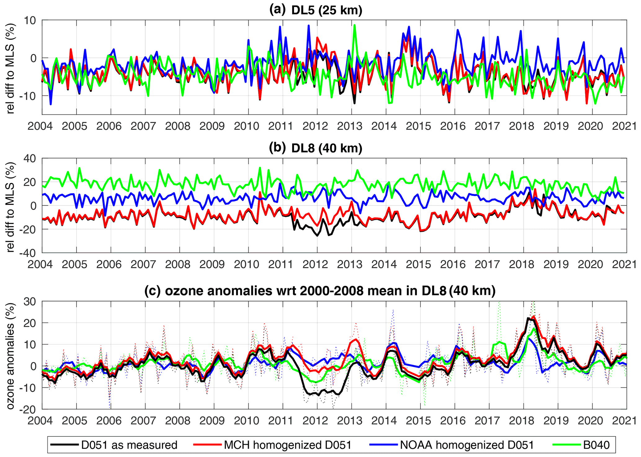
Figure 5 Monthly mean ozone content relative difference to Aura MLS of Dobson D051 as measured (black), Dobson D051 NOAA homogenized (blue), Dobson D051 MCH homogenized (this study, red) and Brewer B040 (green) deseasonalized time series in (a) DL5 and (b) DL8. (c) Time series of ozone anomalies towards their 2000–2008 mean for the same ground-based datasets in DL8.

In order to evaluate the effects of both homogenization on the Dobson D051 time series, monthly mean relative difference to Aura MLS data record are plotted in Fig. 5 for two altitude levels, i.e., DL5 (25 km) in the middle stratosphere and DL8 (40 km) in the upper stratosphere. The relative difference of the Brewer B040 time series is also shown for the same layers.

The Brewer B040 relative difference shows a constant offset to Aura MLS but clear anomalies in 2012 and 2013 in DL5 (Fig. 5a). The Dobson D051 homogenized by NOAA shows a very good accordance with Aura MLS both in DL5 and DL8. The small mean bias is a result of the NOAA optimization of the stray light correction. Therefore, it is not the magnitude of the bias between the homogenized dataset and Aura MLS but its variation (the bias should be constant) which should be considered here. No clear offset in the difference to Aura MLS between the NOAA and the MCH homogenized record is reported in DL5. The variability of the differences to Aura MLS of each dataset looks higher after 2010, while the mean values are constant. However, the slight underestimation of the MCH homogenization since 2017 seems to match the Brewer B040 difference to Aura MLS in DL5 (Fig. 5a). After 2017, the relative difference to Aura MLS of D051 homogenized by MCH and of the collocated B040 is within −5 % to −10 % while the D051 homogenized by NOAA lies within −2 % of Aura MLS.

A clear correction of the 2011–2013 period is visible in DL8 (Fig. 5b). Except for the respective MCH and NOAA homogenized dataset mean offsets to Aura MLS, a slight overestimation of the NOAA homogenization is visible in 2012 and 2013. However, the Brewer B040 relative difference to Aura MLS is also slightly smaller during this time range, when the Brewer instrument had not undergone any technical interventions. This is particularly visible on the anomalies time series of B040 in Fig. 5c. As the MCH homogenization relies on the Brewer collocated datasets, it allows the local variability of the ozone DL8 content to be taken into account, which the M2GMI model, basis for the NOAA homogenization, probably does not consider. As the atmospheric processes are more homogenized in the stratosphere than in the troposphere, the M2GMI ozone profiles should be representative of stratospheric ozone variability. Nevertheless, it is possible that other atmospheric interferences (i.e., aerosols) can impact the Dobson readings of zenith sky radiance which would also impact Brewer observations but might not be fully included in the M2GMI simulations.

Due to the occurrence of an anomaly in 2018, which is particularly visible in DL8 for all datasets (Fig. 5c), the last correction applied to the dataset by the NOAA and the MCH homogenization differs.

As the MCH homogenization considers a step correction in May 2018, the ozone increase during the 2018 anomaly is accounted for in the mean difference of the D051 dataset to the Brewers datasets of the pre- and post-step periods. As a result, the calculated offset is small. The NOAA homogenization method detects a change in the Umkehr ozone with respect to the M2GMI record that starts a year earlier, in 2017. The ozone increase during the 2018 anomaly is only accounted for in the mean difference to M2GMI of the post-step period of the D051 dataset. Moreover, this post-step difference is overestimated as M2GMI does not seem to simulate any significant anomaly at that period. As a result, the calculated offset, applied in 2017, is probably overestimated.

Now that the Dobson D051 is fully homogenized, vertically resolved long-term trends can be estimated with limited influence of instrumental artifacts.

4 Long-term trend estimation methods

Two regression methods for trend estimation are described in this section. First, we describe the common and widely used MLR, and second, we detail the more recent DLM regression method. Trend estimations by both methods are then compared for the case study of the MCH homogenized Dobson D051 dataset.

4.1 MLR trend estimation method

Trends are estimated by fitting a multilinear regression function to the monthly mean ozone time series considering two piecewise linear trends (PWLT) starting in 1970 and in 1998. Trend profiles are obtained by considering one independent monthly mean time series for each pressure level. The results are given as a difference in DU to the 1970–1980 and of the 2000–2010 means. The explanatory variables represent sources of geophysical variability with known influence on stratospheric ozone, including the quasi-biennial oscillation (from https://www.geo.fu-berlin.de/met/ag/strat/produkte/qbo/index.html, last access: 26 July 2022) (QBO) at 30 and 10 hPa, the 10.7 cm solar radio flux describing the 11-year solar cycle (from https://www.iup.uni-bremen.de/UVSAT/Datasets/mgii, last access: 26 July 2022) (SOL), the El Niño–Southern Oscillation (from http://www.esrl.noaa.gov/psd/enso/mei/, last access: 26 July 2022) (ENSO), the North Atlantic Oscillation (from https://climatedataguide.ucar.edu/climate-data/hurrell-north-atlantic-oscillation-nao-index-station-based, last access: 28 November 2021) (NAO), the stratospheric aerosol optical depth (from https://asdc.larc.nasa.gov/project/GloSSAC/GloSSAC_1.0, last access: 28 Novemeber 2021) (SAOD) and Fourier components representing the seasonal cycle (annual and semi-annual variations). All data points are considered with equal weights, and the uncertainty of the fit parameters is estimated from the regression residuals. Residual autocorrelations are accounted for by applying a Cochrane–Orcutt transformation to the model (Cochrane and Orcutt, 1949).

4.2 DLM trend estimation method

Dynamical linear modeling allows for the determination of a nonlinear time-varying trend from a monthly mean time series. This is a Bayesian approach regression which fits the data time series for a nonlinear time-varying trend, regression coefficients from explanatory variables, and seasonal and annual modes, considering their uncertainties and an autoregressive component. The trend is allowed to smoothly vary in time, and its degree of nonlinearity is inferred from the data, as well as the turnaround period. We use the code by Alsing (2019), which is a Python implementation of the formalism introduced by Laine et al. (2014), and we refer to these publications for a detailed description of the DLM principles. The model used considers standard regression components, allows for a variability of the sinusoidal seasonal modes and includes the autoregressive (AR1) correlation process with variance and correlation coefficient as free parameters in the regression. The same five explanatory variables as in the MLR are used in the trend estimate: QBO at 30 and 10 hPa, SOL, ENSO and SAOD NH values. The estimation of the posterior uncertainty distribution is performed with the Markov chain Monte Carlo (MCMC) method and considers the uncertainties on the regression components, on the seasonal cycle, on the autoregressive correlation and on the nonlinearity of the trend. Note that only statistical uncertainties are given in the paper, which allows the significance of the trends to be determined. In order to check the agreement of trends derived form different datasets, uncertainties including a term accounting for remaining steps and for inhomogeneities in the dataset (Bernet et al., 2021) should be considered.

Figure 6 (a–c) DLM (in blue) and MLR (in black) trend estimates in percent per decade ± 2σ of the Dobson D051 dataset for three DLs between 20 and 40 km. The shaded areas show the 2σ uncertainties. (d–f) The distribution of the DLM trend estimates is given by the kernel density estimation (KDE) for the same three DLs in the 1998–2020 time range in Dobson units ± FWHM.

4.3 Comparison of MLR and DLM trend estimation: case of Dobson D051 dataset

Figure 6 shows the long-term trend estimates from the MCH homogenized Dobson D051 dataset by DLM (in blue with ± 2σ uncertainty shaded area) and by MLR (PWLT, in black with ± 2σ uncertainty shaded area) for the same explanatory variables at three altitude levels. The blue shaded areas show the non-constant 2σ uncertainties in Dobson units per year estimated by the DLM. By analogy, for the MLR, the grey shaded areas report the uncertainty in Dobson units per year calculated from the constant 2σ offset trend uncertainty in Dobson units per decade.

Overall trends are similar but differ over short timescales because of their representation of the nonlinearity of the changes in the data record. The advantage of DLM lies in the estimation of a smoothly varying trend without assuming any shape. The inflection year depends on the method: while the inflection point is fixed by the MLR PWLT (1998 in this case; see Petropavlovskikh et al., 2019), the inflection year is retrieved by the DLM and results in year 2002 for the Dobson D051 dataset above 28 km. The maximum of the ΔO₃ (ozone difference) between 1998–2020 KDE (kernel density estimation) should be compared to the linear trend value over the same time period (22 years), while the 95 % level of significance, represented by the fraction of the KDE above/below zero, slightly differs from the MLR uncertainty estimates. In the lower stratosphere, for DL4 (Fig. 6a and d), the post-1998 MLR trend values are −0.33 ± 1.35 % per decade. The DLM KDE shows a maximum at −1.64 DU and a full width at half maximum (FWHM) (i.e., 2.4σ for normal distribution) of 1.81 DU, which means a mean trend of −1.09 ± 1.10 % per decade. The MLR estimate is nonsignificantly different from zero at the 95 % confidence level, while the DLM estimate is negative and barely significant at the 95 % level. In the middle stratosphere, for DL5 (Fig. 6b and e), the post-1998 MLR trend values are −0.52 ± 0.86 % per decade. The DLM KDE shows a maximum at −1.49 DU and a FWHM of 1.18 DU, which means a mean trend of −1.09 ± 0.78 % per decade. The MLR estimate is nonsignificantly different from zero at the 95 % confidence level, while the DLM estimate is significantly negative at the 95 % level. In the upper stratosphere, for DL8 (Fig. 6c and f), the post-1998 MLR trend values are +4.84 ± 1.40 % per decade, and the DLM KDE shows a maximum at +0.80 DU and a FWHM of 0.41 DU, which means a mean trend of +3.59 ± 1.69 % per decade. Both are significantly positive at the 95 % confidence level. The estimated post-1998 MLR trends are in agreement with the vertically resolved trends reported in the literature (Godin-Beekmann et al., 2022), and the post-1998 MLR and DLM estimated trends are in agreement within their uncertainties. The lower and middle stratospheric trends differ in their significance though. In case of high annual variability, a DLM trend estimate in percent per decade may be significant, while a MLR trend estimate may be nonsignificant for the same considered period. Note that the given DLM trend value in percent per decade is an average of the percentage change per year. The regressions (resulting trends and their uncertainties) are influenced by outliers (Bowerman and O'Connell, 1990), but trends estimated by DLM regression change each year. Hence, outliers only influence a limited portion of the DLM trend time series, influencing only the associated trend uncertainties.

5 Long-term trend estimation results

Post-2000 vertically resolved ozone trends for the Arosa/Davos station are estimated by DLM on the MCH and the NOAA homogenized Dobson D051 Umkehr dataset, on the Brewer B040 Umkehr dataset and on the Aura MLS dataset for overpasses over the station.

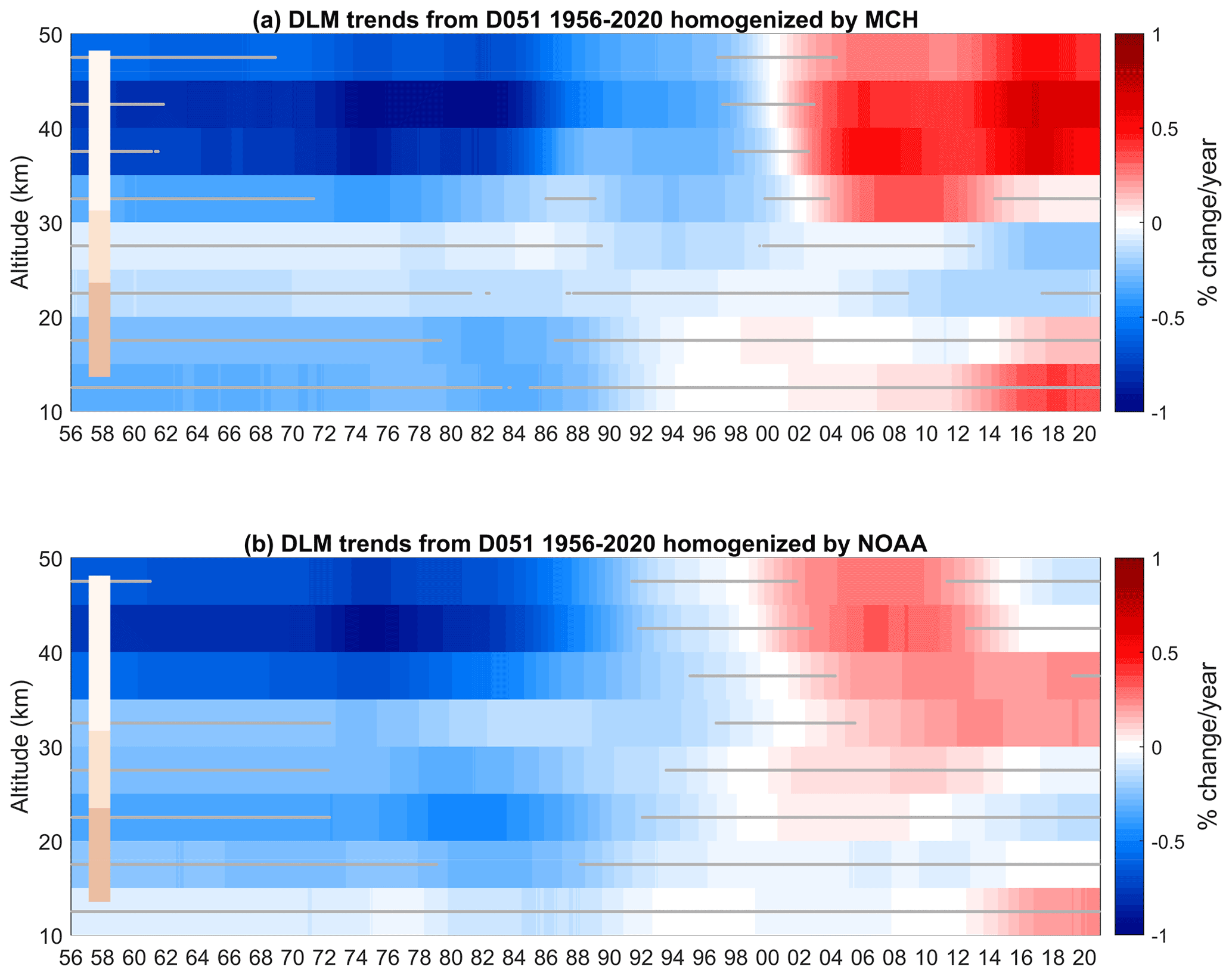
Figure 7 DLM trend estimates in percent per year of Dobson D051 1956–2020 from (a) MCH homogenized and (b) NOAA homogenized data records. Grey lines indicate trend estimates nonsignificantly different from zero at the 95 % confidence level. The beige bars indicate the lower, middle and upper stratospheric ranges.

5.1 Vertically resolved ozone trends derived from the two homogenized Dobson D051 datasets

Figure 7a and b show the DLM trend estimates derived from the Dobson D051 record as homogenized by MCH (Fig. 7a) and by NOAA (Fig. 7b). The trend values are given in percent change per year for each altitude level between 10 and 50 km. Positive and negative trends are shown with varying intensities of red and blue, respectively. The grey lines indicate trend estimates nonsignificantly different from zero at the 95 % confidence level.

The upper stratospheric (DL7–10, 10–1 hPa, 35–50 km) trend estimates are significantly negative between 1965 and 1997 in Fig. 7a and before 1997 in Fig. 7b. The mean negative trend estimates are −5 % per decade (mean value of the 1965–1997 upper stratospheric trends). Both records then show a transition period until 2003, with nonsignificant upper stratospheric trend estimates. The post-2003 upper stratospheric trends are significant and positive, up to 2020 for the MCH homogenized Dobson D051 record and until 2013 for the NOAA homogenized Dobson D051 record. The mean positive upper stratospheric trends are 3.6 % per decade in Fig. 7a (mean value of the 2003–2013 upper stratospheric trends) and 2.1 % per decade in Fig. 7b (mean value of the 2003–2013 upper stratospheric trends). Note that due to the large AKs of the Umkehr measurement, the ozone and trend information in DL8 and DL9 is not independent of each other. In the middle stratosphere (DL5 and 6, 24–32 km), both homogenized records show a negative trend in DL5, persistent and significantly different from zero at the 95 % confidence level since 2012 for the MCH homogenized Dobson D051 data record but slightly positive between 2002 and 2010 and nonsignificantly different from zero at the 95 % confidence level for the NOAA homogenized data record. In the lower stratosphere (LS; DL3 and 4, 14–24 km), the DL3 and DL4 trend estimates are nonsignificantly negative before 1996 but significantly negative between 2008 and 2018 in DL4 for the MCH homogenized data record and nonsignificantly negative for the NOAA homogenized Dobson D051 record.

Again due to the AK width of the Umkehr profiles, the ozone content information of DL2 partly overpasses the lower stratosphere as usually defined (see representation of shaded areas in Fig. 1b). The same consideration is true for the DL6 in the middle stratosphere. The lower part of the lower stratosphere and the upper part of the middle stratosphere trends may be aliased by upper tropospheric and upper stratospheric information, respectively.

Figure 8 Post 2000 DLM trend estimates in percent per year from (a) Dobson D051, (b) Brewer B040 and (c) Aura MLS data records. Grey lines indicate trend estimates nonsignificantly different from zero at the 95 % confidence level. The beige bars indicate the lower, middle and upper stratospheric ranges.

5.2 Vertically resolved ozone trends derived from the Dobson D051, the Brewer B040 and the Aura MLS datasets

Post-2000 trends have been estimated on the three Dobson and the three Brewer MCH Umkehr data records. The trend estimates of one of the Dobsons (D051), one of the Brewers (B040) and Aura MLS are represented in Fig. 8a–c in percent change per year for each altitude level between 10 and 50 km.

The post-2000 trends show similar features for the Dobson and Brewer spectrophotometers:

• There is a positive trend of 0.2 to 0.5 % yr⁻¹ above 35 km, significant for Dobson D051 (and for Dobson D062 and Brewer B156 not shown) but lower and therefore nonsignificantly different from zero at the 95 % level of confidence for Brewer B040 and Dobson D101. Despite differences in the trend estimate intensities, an overall picture of a upper stratospheric positive trend after 2002 is shown.

• There is a persistent negative trend in DL5 of the middle stratosphere and DL4 of the lower stratosphere, with different levels of significance depending on the dataset but mostly nonsignificantly different from zero at the 95 % confidence level except for Dobson D051.

Significant upper stratospheric positive trends are estimated on the Aura MLS satellite data record (Fig. 8c) but have been nonsignificant since 2013. Signs of negative trends in the lower altitudes are also observed although not significant: DLM trend estimates have been persistently negative in the middle stratosphere and negative in the lower stratosphere since 2012.

6 Conclusions

Data records of six collocated spectrophotometers were intercompared on the raw data level (N values) and on the ozone profile level in order to detect anomalies. The MCH Dobson D051 Umkehr data record has been homogenized on the raw data level by comparison with the collocated Brewer triad data record and with the redundant Dobson data records. In a separate work, a second homogenization of the same Dobson dataset was performed by NOAA, using comparison with the M2GMI model on the raw data level as well. Both homogenization processes result in similar magnitudes of N value corrections relative to the post-2018 values. They differ in the application of a correction for the stray light effect and of a correction of the volcanic eruption periods. By relying on the collocated Brewers datasets, the MCH homogenization accounts for the local variability of the ozone layer content in the 2011–2013 period and results in a smaller correction of the data record for this period. Even if only slightly different, the homogenization processes of the raw data can produce significant differences in ozone profiles and, therefore, in the long-term trend estimates. The two homogenization studies differ in their comparison towards Aura MLS and Brewer B040 on the ozone profiles level in the upper stratosphere, especially for the period 2017–2019.

Trends of the ozone profile time series have been estimated by DLM from the Dobson and the Brewer spectrophotometer datasets. The post-2000 trends show similar features, namely a positive trend of 0.2 to 0.5 % yr⁻¹ above 35 km in the upper stratosphere, significant for Dobson D051 but lower and therefore nonsignificantly different from zero at the 95 % level of confidence for Brewer B040, and a persistent negative trend in DL5 of the middle stratosphere, with different levels of significance depending on the dataset. The DLM trend estimates from Dobson D051 show a significant persistent negative trend in DL5 and also support the mention of a persistent negative trend in the NH lower stratosphere (in DL4) when measured by ground-based instrument, considering, however, that the trends estimates in the upper part of the middle stratosphere and in the lower part of the lower stratosphere are aliased by the large AKs of the Umkehr profiles.

DLM trend estimates derived from Aura MLS show similar features in the upper stratosphere and the middle stratosphere as estimates from the ground-based Dobson and Brewer spectrophotometers. However, a transition from nonsignificant positive to nonsignificant negative trends in the lower stratosphere remains unexplained.

While significant positive trends have been estimated in the upper stratosphere since 2004 from the MCH homogenized Dobson D051 dataset, the trend estimates from the NOAA homogenized data record appear to show a transition from significant positive to nonsignificant negative/zero values above 40 km in 2016. Further investigation will be needed to confirm this transition and exclude 2017 as a problematic period in the NOAA homogenization.

Both homogenization approaches considered in this study are relevant and significantly improve the Dobson D051 data record. However, inconsistencies in the level of significance of the Dobson D051 trend estimates are noticed and should be attributed to the remaining differences left by the homogenization processes in the data records.