the Creative Commons Attribution 4.0 License.
the Creative Commons Attribution 4.0 License.
 | 08 Sep 2022
Model output statistics (MOS) applied to Copernicus Atmospheric Monitoring Service (CAMS) O3 forecasts: trade-offs between continuous and categorical skill scores
Dene Bowdalo
Pierre-Antoine Bretonnière
Marc Guevara
Oriol Jorba
Jan Mateu Armengol
Margarida Samso Cabre
Kim Serradell
Albert Soret
Carlos Pérez Garcia-Pando
Air quality (AQ) forecasting systems are usually built upon physics-based numerical models that are affected by a number of uncertainty sources. In order to reduce forecast errors, first and foremost the bias, they are often coupled with model output statistics (MOS) modules. MOS methods are statistical techniques used to correct raw forecasts at surface monitoring station locations, where AQ observations are available. In this study, we investigate the extent to which AQ forecasts can be improved using a variety of MOS methods, including moving average, quantile mapping, Kalman filter, analogs and gradient boosting machine methods, and consider as well the persistence method as a reference. We apply our analysis to the Copernicus Atmospheric Monitoring Service (CAMS) regional ensemble median O3 forecasts over the Iberian Peninsula during 2018–2019. A key aspect of our study is the evaluation, which is performed using a comprehensive set of continuous and categorical metrics at various timescales, along different lead times and using different meteorological input datasets.
Our results show that O3 forecasts can be substantially improved using such MOS corrections and that improvements go well beyond the correction of the systematic bias. Depending on the timescale and lead time, root mean square errors decreased from 20 %–40 % to 10 %–30 %, while Pearson correlation coefficients increased from 0.7–0.8 to 0.8–0.9. Although the improvement typically affects all lead times, some MOS methods appear more adversely impacted by the lead time. The MOS methods relying on meteorological data were found to provide relatively similar performance with two different meteorological inputs. Importantly, our results also clearly show the trade-offs between continuous and categorical skills and their dependencies on the MOS method. The most sophisticated MOS methods better reproduce O3 mixing ratios overall, with the lowest errors and highest correlations. However, they are not necessarily the best in predicting the peak O3 episodes, for which simpler MOS methods can achieve better results. Although the complex impact of MOS methods on the distribution of and variability in raw forecasts can only be comprehended through an extended set of complementary statistical metrics, our study shows that optimally implementing MOS in AQ forecast systems crucially requires selecting the appropriate skill score to be optimized for the forecast application of interest.
- Article
(15904 KB) - Full-text XML
- BibTeX
- EndNote


Air pollution is recognized as a major health and environmental issue (World Health Organization, 2016). Mitigating its negative impacts on health requires reducing both pollutant concentrations and population exposure. Air quality (AQ) forecasts can be used to warn the population of the potential occurrence of a pollution episode while allowing the implementation of temporary emission reductions, including, for example, traffic restrictions, shutdown of industries and bans on the use of fertilizers in the agricultural sector.
AQ forecasting systems are typically based on regional chemistry-transport models (CTMs), which remain subject to numerous uncertainty sources, leading to persistent systematic and random errors, especially for ozone (O3) and particulate matter (PM) (e.g., Im et al., 2015a, b). More importantly, they often largely underestimate the strongest episodes that exert the worst impacts upon health. In addition to the error sources related to the models themselves and the input data, part of the discrepancies between in situ observations and geophysical forecasts are due to inherent representativeness issues since concentrations measured at a specific location are not always comparable to the concentrations simulated over a relatively large volume.
To overcome these limitations, operational AQ forecasting systems based on geophysical models often rely on so-called model output statistics (MOS) methods for statistically correcting the raw forecasts at monitoring stations. The basic idea of MOS methods is to combine raw forecasts with past observations, and eventually with other ancillary data, at a given station in order to produce a better forecast, preferably at a reasonable computational cost. As these MOS methods often significantly reduce systematic errors, bringing mean biases close to zero, they are also commonly referred to as bias-correction or bias-adjustment methods, although they may not be aimed at directly reducing this specific metric. MOS methods relying on local data (first and foremost the local observations) can also be seen as so-called downscaling methods since they allow some of the local features that cannot be reproduced at typical CTM spatial resolution to be captured.
Over the last decades, several MOS methods have been proposed for correcting weather forecasts, before their more recent application to AQ forecasts, essentially on O3 and fine particulate matter (PM2.5, with aerodynamic diameter lower than 2.5 µm). A very simple approach consists of subtracting the mean bias (or multiplying by a mean ratio to avoid negative values in the corrected forecasts) calculated from past data (McKeen et al., 2005). A more adaptive version consists of correcting the forecast by the model bias calculated over the previous days, which assumes some persistence in the errors (Djalalova et al., 2010). Other authors proposed fitting linear regression models between chemical concentration errors and meteorological parameters (e.g., Honoré et al., 2008; Struzewska et al., 2016). Liu et al. (2018) applied a set of autoregressive integrated moving average (ARIMA) models to improve Community Multiscale Air Quality (CMAQ) model forecasts. The Kalman filter (KF) method is a more sophisticated approach, yet still relatively simple to implement, based on signal processing theory (e.g., Delle Monache et al., 2006; Kang et al., 2008, 2010; Borrego et al., 2011; Djalalova et al., 2010, 2015; Ma et al., 2018). Initially employed for correcting meteorological forecasts (Delle Monache et al., 2011; Hamill and Whitaker, 2006), the ANalogs (AN) method provides an observation-based forecast using historical forecasts and has recently provided encouraging results for correcting PM2.5 CMAQ forecasts over the United States (Djalalova et al., 2015; Huang et al., 2017).
A common limitation in the aforementioned studies is that MOS corrections are assessed mainly in terms of continuous variables (i.e., pollutant mixing ratios), while typically less attention is put on the parallel impact in terms of categorical variables (i.e., exceedances of given thresholds), which is however one of the primary goals of AQ forecasting systems. This can give a partial, if not misleading, view of the advantages and disadvantages of the different MOS approaches proposed in the literature.
The present study aims at providing a comprehensive assessment of the impact of different MOS approaches upon AQ forecasts. We consider a representative set of MOS methods, including some already proposed in the recent literature and another one based on machine learning (ML). These MOS corrective methods are applied to the Copernicus Atmospheric Monitoring Service (CAMS) regional ensemble O3 forecasts, focusing on the Iberian Peninsula (Spain and Portugal) during the period 2018–2019. The MOS methods are evaluated for a comprehensive set of continuous and categorical metrics, at various timescales (hourly to daily) and along different lead times (1 to 4 d), with different meteorological input data (forecast vs reanalyzed), in order to provide a more complete vision of their behavior.
The paper is organized as follows: Sect. 2 first describes the data and MOS methods used in this study; Sect. 3 includes the evaluation of the raw (uncorrected) CAMS regional ensemble O3 forecast over the Iberian Peninsula, along with a detailed assessment of the MOS results and some sensitivity analyses; and a broader discussion and conclusion are provided in Sect. 4.
2.1 Data
2.1.1 Ozone observations
Hourly O3 measurements over 2018–2019 are taken from the European Environmental Agency (EEA) AQ e-Reporting (EEA, 2020) and accessed through GHOST (Globally Harmonised Observational Surface Treatment). GHOST is a project developed at the Earth Sciences Department of the Barcelona Supercomputing Center that aims at harmonizing global surface atmospheric observations and metadata, for the purpose of facilitating quality-assured comparisons between observations and models within the atmospheric chemistry community (Bowdalo, 2022). On top of the public datasets it ingests, GHOST provides numerous data flags that are used here for quality assurance screening (see Appendix A). In this study, daily mean, daily 1 h maximum and daily 8 h maximum (hereafter respectively referred to as d, d1max and d8max) are computed only when at least 75 % of the hourly data are available (i.e., 18 over 24 h). Note that despite such data availability criteria, large data gaps at some stations and during some days might occur mainly during daytime (for instance due to maintenance operations that typically occur during working hours). Considering all stations and days with at least 18 h of data, the frequency of data gaps exceeding 4 h between 08:00 and 15:00 UTC was found to be only 0.6 % (). Such situations occur with a similarly low frequency on days exceeding the target threshold ( or 0.6 %) and never occur on days exceeding the information threshold.
Our study focuses on the Iberian Peninsula, over a domain ranging from 10° W to 5° E longitude and from 35 to 44° N latitude that includes Spain, Portugal and part of southwestern France. In total, 455 O3 monitoring stations are included, which represents an observational dataset of 7 437 862 hourly O3 measurements with 93 % of hourly data availability.
2.1.2 CAMS regional ensemble forecast
The benefit of MOS corrections is investigated on the CAMS regional ensemble forecasts. As one of the six Copernicus services, CAMS provides AQ forecast and reanalysis data at both regional and global scales (https://www.regional.atmosphere.copernicus.eu/, last access: 20 November 2020). At regional scale, nine state-of-the-art CTMs developed by European research institutions are currently participating in the operational ensemble AQ forecasts (CHIMERE from INERIS, EMEP from MET Norway, EURAD-IM from University of Cologne, LOTOS-EUROS from KNMI and TNO, MATCH from SMHI, MOCAGE from METEO-FRANCE, SILAM from FMI, DEHM from Aarhus University, GEM-AQ from IEP-NRI). In addition, MONARCH from BSC and MINNI from ENEA will join the ensemble soon. The ensemble forecast is computed as the median of all individual forecasts. Note that due to possible technical failures, all nine forecasts are not always available for computing the full ensemble. The CAMS regional forecasts are provided over 4 lead days, hereafter referred to as D+1, D+2, D+3 and D+4 (starting at 00:00 UTC).
2.1.3 HRES and ERA5 meteorological data
Some MOS methods rely on meteorological data. In this study, meteorological data are taken from the Atmospheric Model high-resolution 10 d forecast (HRES) (https://www.ecmwf.int/en/forecasts/datasets/set-i, last access: 1 September 2020) provided by the European Centre for Medium-Range Weather Forecasts (ECMWF). HRES has a native spatial resolution of about 9 km and 137 vertical levels. In addition, to investigate the sensitivity to the meteorological input data, we replicated all our experiments with the ERA5 reanalysis dataset (Copernicus Climate Change Service (C3S), 2017; https://www.ecmwf.int/en/forecasts/datasets/reanalysis-datasets/era5, last access: 1 September 2020). ERA5 data have a native spatial resolution of about 31 km and 137 vertical levels, although data were downloaded on a 0.25° × 0.25° regular longitude-latitude grid from the Climate Data Store. At all surface O3 monitoring stations, for both HRES and ERA5, we extracted the following variables at the hourly scale: 2 m temperature (code 167), 10 m surface wind speed (207), normalized 10 m zonal and meridian wind speed components (165 and 166), surface pressure (134), total cloud cover (164), surface net solar radiation (176), surface solar radiation downwards (169), downward UV radiation at the surface (57), boundary layer height (159), and geopotential at 500 hPa (129).
2.2 Applying MOS under restrictive operational conditions
A novel aspect of this study is that we provide a comparison of a set of MOS methods under potentially restrictive training conditions in operational context. To mimic such restrictions we assume that (1) no past data, neither modeled nor observed, are available for training at the beginning of the period of study (here 1 January 2018) and (2) the number of modeled and observed data continuously grows with time along the period of study (here 2018–2019). On a given day, the MOS methods can therefore only rely on the historical data accumulated since the beginning of the period. Our approach consists of understanding the behavior of the different MOS methods in a worst-case scenario where a new or upgraded operational AQ forecasting system is implemented together with a MOS module for which there are few or no hindcast data. We believe that such a strategy allows the different MOS methods to be compared in a balanced way given the operational context. As described in detail in the next section, some MOS methods require very limited prior information to achieve their optimal performance, while others need a larger number of training data. In an operational context, the first category of methods might thus be advantaged at the beginning before being gradually supplanted with the second category. We note, however, that methods relying on limited past data may respond better to an abrupt change in environmental conditions, as experienced for instance during the COVID-19 lockdowns. Although not covered by the present study, we acknowledge here that in an operational context, the relationship between the length of past training data and the performance of the corresponding MOS prediction is an interesting aspect to investigate, as is the quantification of the spin-up time beyond which the MOS method might not significantly improve. Only some insights will be given by comparing the performance obtained in 2019 with and without using the data available in 2018. Similarly, our study does not investigate how potential issues (delays) in the near-real-time availability of the observations can impact the performance of the MOS methods, although this might be another important aspect to take into account in operational conditions; to the best of our knowledge, EEA observations are typically available with a 2 h lag, but some sporadic technical failures can induce extended delays.
2.3 Description of the model output statistics (MOS) methods
This section describes the different MOS methods implemented for correcting the raw forecasts (hereafter referred to as RAW), namely moving average (MA), Kalman filter (KF), quantile mapping (QM), analogs (AN) and gradient boosting machine (GBM) methods. All MOS methods are applied independently at each monitoring station. The skill of these different forecasts (including the RAW) is assessed relative to the persistence (PERS) reference method, which uses the previously observed concentration values at a specific hour of the day (averaged over 1 or several days) as the predicted value. As a first approach, we use a time window of 1 single day (hereafter referred to as PERS(1)).
2.3.1 Moving average (MA) method
We primarily consider the moving average (MA) method, by which the raw CAMS forecast bias in the previous day(s) is used to correct the forecast. As a first approach, we use a time window of 1 single day (hereafter referred to as MA(1)). The sensitivity to the time window is discussed in Sect. 3.4.
2.3.2 Quantile mapping (QM) method
The quantile mapping (QM) method aims at adjusting the distribution of the forecast concentrations to the distribution of observed concentrations. For a given day, the QM method consists of (1) computing two cumulative distribution functions (CDFs), corresponding to past modeled and observed O3 mixing ratios, respectively; (2) locating the current O3 forecast in the model CDF; and (3) identifying the corresponding O3 values in the observation CDF and using it as the QM-corrected O3 forecast. For instance, if the current O3 forecast gives a value corresponding to the 95th percentile, the QM-corrected O3 forecast will correspond to the 95th percentile of the observed O3 mixing ratios. This approach thus aims at correcting all quantiles of the distribution, not only the mean.
In the operational-like context in which this study is conducted (Sect. 2.2), the first QM corrections are computed when 30 d of data have been primarily accumulated to ensure a minimum representativeness of the model and observation CDFs. For computational reasons, both CDFs are updated every 30 d (although an update frequency of 1 single day would be optimal in a real operational context). The choice of a 30 d update frequency only aims at reducing the computational cost of running all MOS methods at all stations during the 2-year period. In a real operational context, only 1 d would have to be run, which would allow the update frequency to be increased up to 1 d; i.e., the CDFs would be updated every day, ensuring that we are taking advantage from the entire observational dataset available at a given time.
2.3.3 Kalman filter (KF) method
The Kalman filter (KF) is an optimal recursive data processing algorithm with numerous science and engineering applications (see Pei et al., 2017, for an introduction). In atmospheric sciences, it offers a popular framework for sophisticated data assimilation applications (e.g., Gaubert et al., 2014; Di Tomaso et al., 2017) but can also be used as a simple yet powerful MOS method for correcting forecasts (e.g., Delle Monache et al., 2006; Kang et al., 2008; De Ridder et al., 2012). The KF-based MOS method aims at recursively estimating the unknown forecast bias (here taken as the state variable of interest), combining previous forecast bias estimates with forecast bias observations. The updated forecast bias estimate is computed as a weighted average of these two terms, both being considered to be uncertain, i.e., affected by a noise with zero mean and a given variance. A detailed description of the KF algorithm can be found in Appendix B, but an important aspect to be mentioned here is that each of these two terms is weighted according to the value of the so-called Kalman gain that intrinsically depends on the ratio of both variances (hereafter referred to as the variance ratio). The value chosen for this internal parameter substantially affects the behavior of the KF, and thus the obtained MOS corrections. A variance ratio close to zero induces a Kalman gain close to 0. In such situations, the estimated forecast bias corresponds to the estimated forecast bias of the previous day, independently of the forecast error. A very high (infinite) variance ratio gives a Kalman gain close to 1. In this case, the estimated forecast bias corresponds to the observed forecast bias of the previous day, which thus makes it equivalent to the MA(1) method.
In this study, the variance ratio is adjusted dynamically and updated regularly in order to optimize a specific statistical metric, in our case the RMSE (the corresponding approach being hereafter referred to as KF(RMSE)). The different steps are (1) at a given day of update, the KF corrections over the entire historical dataset are computed considering different values of variance ratio, from 0.001 to 100 in a logarithmic progression; (2) the RMSE is computed for each of the corrected historical time series obtained; and (3) the variance ratio associated with the best RMSE is retained and used until the next update. Other choices of metrics to optimize are explored in Sect. 3.4.
As for QM, for computational reasons, the update frequency is set to 30 d in this study (although, again, an update frequency of 1 single day would be optimal).
2.3.4 Analogs (AN) method
The analogs method (AN) implemented here consists of (1) comparing the current forecast to all past forecasts available, (2) identifying the past days with the most similar forecast (hereafter referred to as analog days or analogs) and (3) using the corresponding past observed concentrations to estimate the AN-corrected O3 forecast (e.g., Delle Monache et al., 2011, 2013; Djalalova et al., 2015; Huang et al., 2017). The current forecast is compared to each individual past forecast in order to identify which ones are the most similar. Based on a set of features including the raw O3 mixing ratio forecast from the AQ model and the 10 m wind speed, 2 m temperature, surface pressure and boundary layer height forecast from the meteorological model, the distance metric proposed by Delle Monache et al. (2011) and previously used in Djalalova et al. (2015) (see the formula in Appendix C) is used to compute the distance (i.e., to quantify the similarity) of each individual past forecast with respect to the current forecast. Then, as a first approach, the 10 best analog days that correspond here to the 10 most similar past forecasts are identified (hereafter referred to as AN(10); other values are tested in Sect. 3.4). From those best analog days, the MOS-corrected forecast is computed as the weighted average of the corresponding observed concentrations, where weights are taken as the inverse of the distance metric previously computed. In comparison to a normal average, introducing the weights is expected to slightly reduce the dependence upon the number of analog days chosen.
Therefore, in the analogs paradigm, the past days of similar chemical and/or meteorological conditions are identified in the forecast (i.e., model) space, while the output (i.e., the AN-corrected forecast) is taken from the observation space. The AQ model thus only serves to identify the past observed situations that look similar to the current one.
2.3.5 Machine-learning-based MOS method
We also explore the use of ML algorithms as an innovative MOS approach for correcting AQ forecasts. In ML terms, it corresponds to a supervised regression problem where a ML model is trained to predict the observed concentrations, hereafter referred to as the target or output, based on multiple ancillary variables, hereafter referred to as the features or inputs, coming from meteorological and chemistry-transport geophysical models and/or past observations. In this context, the use of ML is of potential interest because (i) we suspect that some relationships exist between the target variable and at least some of these features, (ii) these relationships are likely too complex to be modeled in an analytical way, and (iii) data are available for extracting (learning) information about them. Over the last years, ML algorithms became very popular for many types of predictions, notably due to their ability to model complex (typically non-linear and multi-variable) relationships with good prediction skills. Among the myriad of ML algorithms developed so far, we focus on the decision-tree-based ensemble methods, and more specifically on the gradient boosting machine (GBM), which often gives among the best prediction skills (as shown in various ML competitions and model intercomparisons; e.g., Caruana and Niculescu-Mizil, 2005).
At each monitoring station, one single ML model is trained to forecast O3 concentrations at all lead hours (from 1 to 96) or days (from 1 to 4), depending on the timescale used (see Sect. 2.4). The features taken into account include a set of chemical features (raw forecast O3 concentration, O3 concentration observed 1 d before), meteorological features (2 m temperature, 10 m surface wind speed, normalized 10 m zonal and meridian wind speed components, surface pressure, total cloud cover, surface net solar radiation, surface solar radiation downwards, downward UV radiation at the surface, boundary layer height, and geopotential at 500 hPa, all forecast by the meteorological model) and time features (day of year, day of week, lead hour). Although the past O3 observed concentration corresponds to recursive information that will not be available for all forecast lead days, we use here the same value for all lead days. The tuning of the GBM models is described in Appendix D.
As for QM, the GBM model is first trained (and tuned) only after 30 d to accumulate enough data and then retrained every 30 d based on all historical data available.
2.4 Timescales of MOS corrections
Current AQ standards are defined according to pollutant-dependent timescales, e.g., daily 8 h maximum (d8max) concentration in the case of O3. In the literature, MOS corrections are typically applied to hourly concentrations, providing hourly corrected concentrations from which the value at the appropriate timescale can then be computed. Following this approach, for a given MOS method X, corrections in this study are first computed based on hourly time series (hereafter referred to as Xh), from which daily 24 h average (Xd), daily 1 h maximum (Xd1max) and daily 8 h maximum (Xd8max) corrected concentrations are then deduced. In addition, MOS corrections are computed directly on daily 24 h average (Xdd, the additional “d” indicating that the MOS method is applied directly on daily rather than hourly time series), daily 1 h maximum (Xdd1max) and daily 8 h maximum (Xdd8max) time series, respectively. When needed, meteorological features are used at the same timescale. This is done to investigate whether applying the MOS correction directly at the regulatory timescale can help to achieve better performance.
2.5 Evaluation metrics and skill scores
In this study, O3 forecasts are evaluated using an extended panel of continuous and categorical metrics to provide a comprehensive view of the impact of the different MOS methods on the predictions. Continuous metrics used to evaluate the O3 concentrations include the following.
-
nMB: normalized mean bias
-
nRMSE: normalized root mean square error
-
PCC: Pearson correlation coefficient
-
slope: slope of the predicted-versus-observed O3 mixing ratio to quantify how well the lowest and highest O3 concentrations are predicted
-
nMSDB: normalized mean standard deviation bias to investigate how well the O3 variability is reproduced by the forecast
Categorical metrics used to evaluate the O3 exceedances beyond certain thresholds include the following.
-
H: hit rate to quantify the proportion of observed exceedances that are correctly detected
-
F: false alarm rate to quantify the proportion of observed non-exceedances erroneously forecast as exceedances
-
FB: frequency bias to investigate the extent to which the forecast is predicting the same number of exceedances as observed (no matter if they are predicted on the correct days)
-
SR: success ratio to show how much of the predicted exceedances are indeed observed
-
CSI: critical success index to quantify the proportion of correctly predicted exceedances when discarding all the corrected rejections
-
PSS: Peirce skill score to investigate the extent to which the forecast is able to separate exceedances from non-exceedances
-
AUC: area under the receiver operating characteristic (ROC) curve to quantify the probability that the forecast predicts higher O3 concentrations during a situation of exceedance compared to a situation of non-exceedance
The formula of these different metrics can be found in Appendix E. Each of them thus highlights a specific aspect of the performance. Regarding categorical metrics, Jolliffe and Stephenson (2011) gave a detailed explanation of the different metric properties desirable for assessing the quality of a forecasting system (see Table 3.4 in Jolliffe and Stephenson, 2011). In this framework, PSS can be considered to be one of the most interesting metrics for assessing the accuracy of the different RAW and MOS-corrected forecasts, given that it gathers numerous valuable properties: (i) truly equitable (all random and fixed-value forecasting systems are awarded the same score, which provides a single no-skill baseline), (ii) not trivial to hedge (the forecaster cannot cheat on their forecast in order to increase PSS), (iii) base-rate-independent (PSS only depends on H and F, which makes it invariant to natural variations in climate, which is particularly interesting in the framework of AQ forecasting, where AQ standards and subsequently the base rate can also change) and (v) bounded (values are comprised within a fixed range). It is worth noting that no perfect metric exists, and PSS (as most other metrics) does not benefit from the properties of non-degeneracy (it tends towards meaningless values for rare events).
In addition, results are also discussed in terms of skill scores, using the 1 d persistence (PERS(1)) as the reference forecast. Skill scores aim at measuring the accuracy of a forecast relative to the accuracy of a chosen reference forecast (e.g., persistence, climatology, random choice). They can be computed as , with X the score of the forecast, Xreference the score of the PERS(1) reference forecast and Xperfect the score expected with a perfect forecast. Skill scores indicate if a given forecast has a perfect skill (value of 1), a better skill than the reference forecast (value between 0–1), a skill equivalent to the reference forecast (value of 0) or a worse skill than the reference (value below 0, unbounded). To be converted into skill scores, the aforementioned metrics of interest need to be transformed into scores following the rule “the higher the better” (to constrain the skill score to values below 1). For the different metrics M, the corresponding score X(M) is obtained applying the following transformations: for nRMSE and for slope; no transformations are required for the other metrics (H, F, SR, CSI, PSS and AUC). Note that, as indicated by its name, PSS is already intrinsically defined as a skill score (where the reference corresponds to a climatology or random choice, both giving PSS values tending toward 0), but it does not prevent it from being converted into a skill score related to the persistence forecast.
In order to ensure fair comparisons between observations and all the different forecasts, O3 values at a given hour are discarded when at least one of these different dataset does not have data. Over the 2018–2019 period, the resulting data availability exceeds 94 % whatever the timescale considered. Note that about 4 % of the data are missing here due to the aforementioned minimum of 30 d (i.e., January 2018) of accumulated historical data requested to start computing the corrected forecasts with some MOS methods.
We first briefly describe the O3 pollution over the Iberian Peninsula as observed by the monitoring stations and simulated by the CAMS regional ensemble forecast (Sect. 3.1). Then, we investigate the performance of the MOS methods on both continuous (Sect. 3.2) and categorical (Sect. 3.3) O3 forecasts. Different sensitivity tests on the MOS methods are performed in Sect. 3.4, including a test on the impact of the input meteorological data on the MOS performance.
3.1 Ozone pollution over the Iberian Peninsula
The European Union sets different standards regarding O3 pollution, including (1) a target threshold of 60 ppbv for the daily 8 h maximum, with 25 exceedances per year allowed on average over 3 years; (2) an information threshold of 90 ppbv for the daily 1 h maximum; and (3) an alert threshold of 120 ppbv for the daily 1 h maximum. In this study, we focus on the first two thresholds and exclude the last one mainly because exceedances of the alert threshold are extremely rare (only 13 exceedances over 314 005 points, i.e., 0.004 %). With such a low frequency of occurrence, such events remain extremely difficult to predict (without predicting too many false alarms).
The mean O3 mixing ratios, as well as the annual number of exceedances, are shown in Fig. 1 for both observations and raw CAMS ensemble forecasts. The time series at the different timescales are shown in Fig. 2. Over the Iberian Peninsula, annual mean O3 mixing ratios range between 10 and 50 ppbv, depending on the type of monitoring station (urban traffic, urban background, rural background), with typically higher levels on the Mediterranean coast compared to the Atlantic one. Over the entire domain and time period, the target (d8max > 60 ppbv) and information (d1max > 90 ppbv) thresholds have been exceeded 13 221 and 274 times, respectively (i.e., 4 % and 0.08 % of the 314 005 points, respectively). These exceedances are well distributed in time along the 2018–2019 period, with 404 d out of 730 d (55 %) with at least one station exceeding the target threshold, and 78 d out of 730 d (11 %) with at least one station exceeding the information threshold. These exceedances are observed over a large part of the peninsula, but with a higher frequency in specific locations, including the surroundings (typically downwind) of the largest cities (e.g., Madrid, Barcelona, Valencia, Lisbon, Porto) and close to industrial areas (e.g., Puertollano, a major industrial hot spot 200 km south of Madrid).

Figure 1Overview of the O3 pollution over the Iberian Peninsula, as observed by monitoring stations (a, c, e) and as simulated by the CAMS regional ensemble D+1 forecasts (b, d, f), showing the mean O3 mixing ratios (a, b) and the number of exceedances of the standard (d8max > 60 ppbv; c, d) and information threshold (d1max > 90 ppbv; e, f) over the period 2018–2019. In order to limit the overlap, stations are plotted here by decreasing value and with decreasing size (lowest values with largest symbols but in background, highest values with smallest symbols but in foreground). For clarity, the stations without any observed or simulated exceedance are omitted.
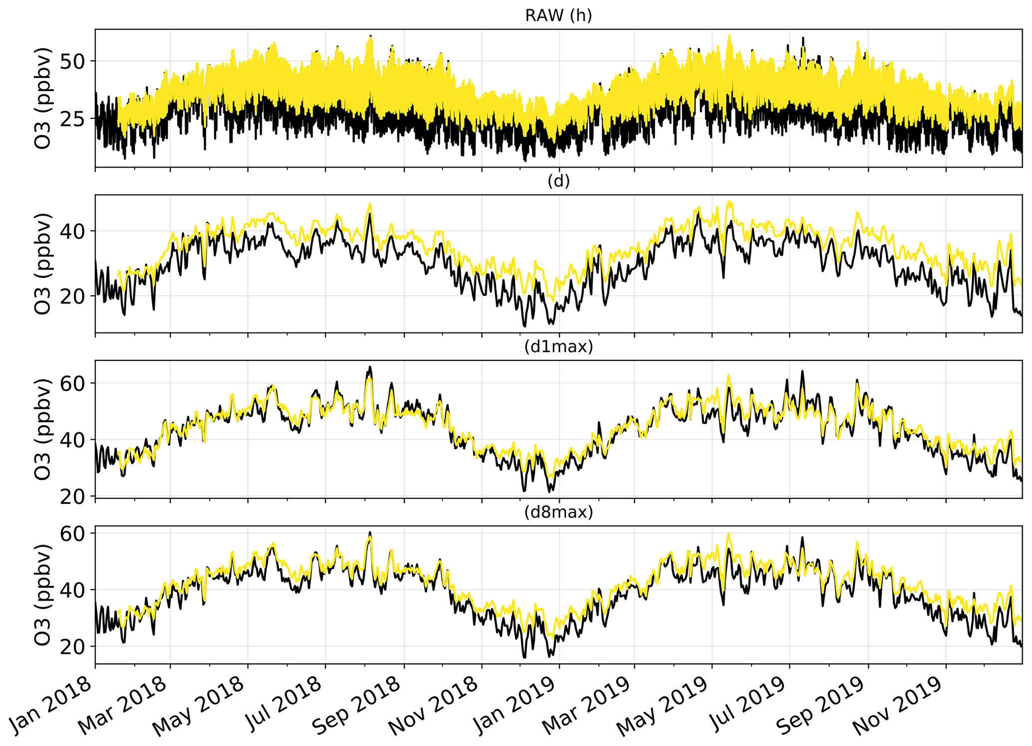
Figure 2Time series of the mean O3 mixing ratios over the Iberian Peninsula, as observed by monitoring stations (in black) and as simulated by the raw CAMS regional ensemble D+1 forecasts (in yellow). Time series are shown at the hourly (h), daily mean (d), daily 1 h maximum (d1max) and daily 8 h maximum (d8max) timescales. O3 mixing ratios are averaged over all surface stations of the domain.
3.2 Performance on continuous forecasts
3.2.1 RAW forecasts
Considering the annual mean O3 mixing ratios at all 456 stations (Fig. 1), the raw CAMS ensemble forecast represents moderately well the spatial distribution of annual O3 over the Iberian Peninsula (PCC of 0.54 for D+1 forecasts) and strongly underestimates the spatial variability (nMSDB of −42 %). At least part of these errors are due to the fact that all station types are taken into account here, including traffic stations where local road transport NOx emissions can strongly reduce the O3 levels (titration by NO), which cannot be properly represented by models at 10 km spatial resolution. In this study, all station types are included because we are ultimately interested in predicting O3 exceedances at all locations where they can be observed (and thus where air quality standards apply). It is worth noting that the impact of the MOS methods on the different metrics might vary from one type of station to another, although this aspect is beyond the scope of our study. The raw CAMS ensemble forecast correctly identifies regions where most exceedances of the target threshold occur but often with underestimated frequency, especially around Madrid, in southern Spain (in-land part of the Andalusia region) and along the Mediterranean coast. More severe deficiencies are found with the information threshold that is almost never reached by the CAMS ensemble (with one single exception around Porto).
The overall statistical results are shown in Fig. 3 for the different forecast methods, and a subset of these statistics is given in Table 1 (and in Table S1 in the Supplement for additional timescales). For a given lead day and timescale, statistics are computed here after aggregating data from all monitoring stations; therefore, statistics of D+1 O3 forecasts at the hourly scale can be based on 730 d × 24 h × 455 stations = 7 971 600 points if there are no data gaps. The RAW forecast moderately overestimates the O3 mixing ratios, especially at hourly and daily timescales, but shows a reasonable correlation at all timescales (above 0.75). However, its main deficiency lies in the underestimated variability (nMSDB around −30 %), which is reflected in the low model-versus-observation linear slope obtained (around 0.5–0.6). The deterioration of the performance of the raw CAMS forecasts with lead time is very low, with hourly scale nRMSE and PCC decreasing from 38 % and 0.75 at D+1 to 39 % and 0.72 at D+4, potentially due to their relatively coarse spatial resolution.
As expected (by construction), the PERS(1) reference forecast gives unbiased O3 forecasts. Due to the temporal auto-correlation of O3 concentrations, reasonable results are obtained at D+1 (nRMSE, PCC and slope of 36 %, 0.74 and 0.74) but quickly deteriorate with the lead time (down to 42 %, 0.65 and 0.64 at D+4). A subset of skill scores with PERS(1) for reference is shown in Fig. 4. Apart from the slope that is always better reproduced by PERS(1), the RAW forecast reaches better skill scores than PERS(1) on both the nRMSE and PCC but only beyond D+1 (with values typically ranging between 0–0.2), and not at all timescales (for instance, PERS(1) systematically shows better RMSE than RAW at the daily scale).
Table 1Evaluation of the different forecast methods on continuous metrics, at D+1 (and D+4 in parentheses), for the h, d, d1max and d8max timescales (see Table S1 in the Supplement for the evaluation results at dd, dd1max and dd8max timescales).
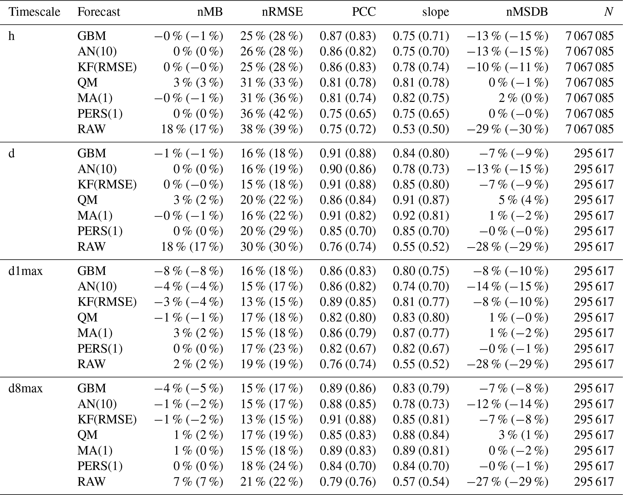
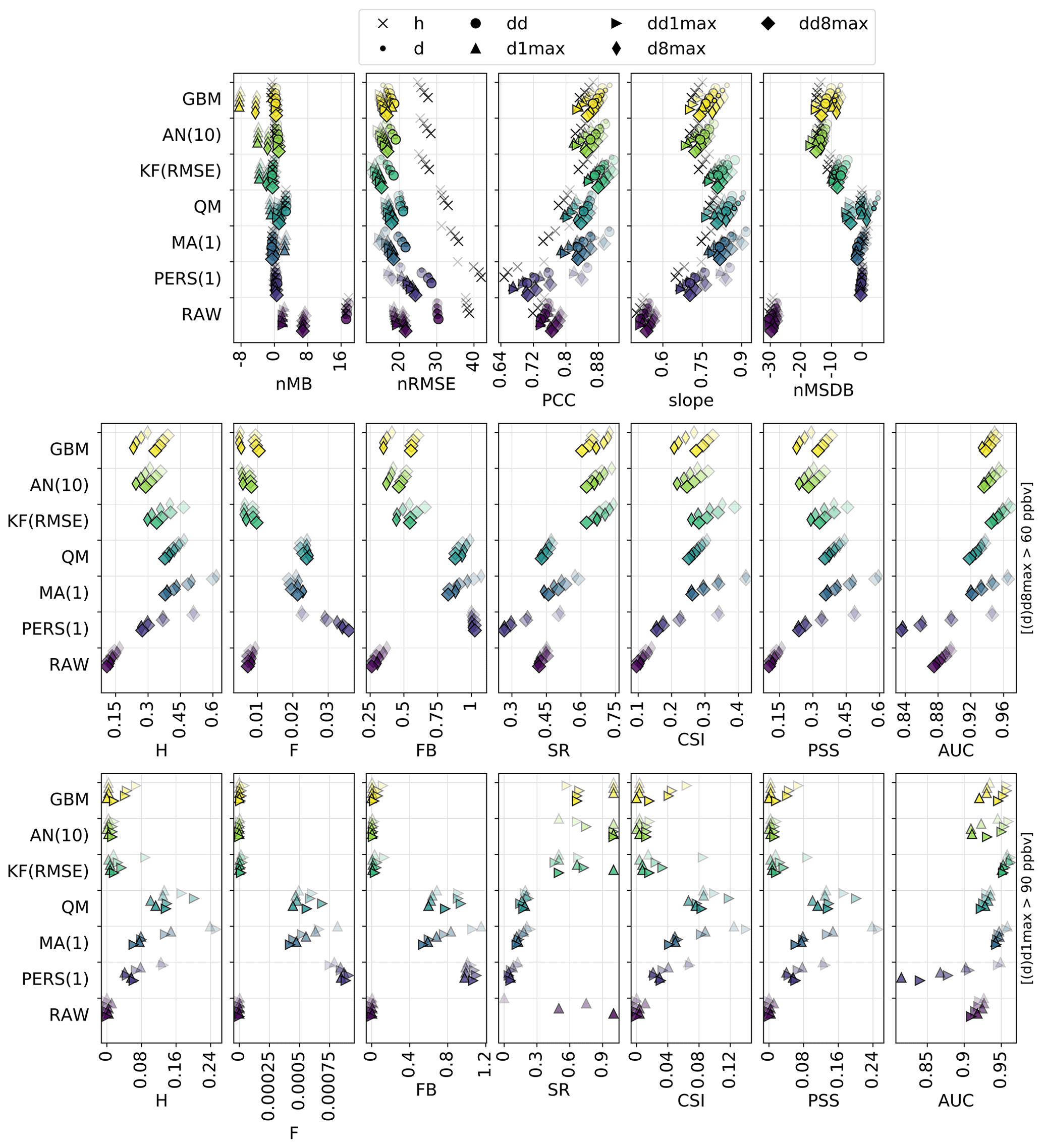
Figure 3Statistical performance of RAW and MOS-corrected CAMS O3 forecasts for continuous metrics (top panels) and categorical metrics related to the exceedance of the target (intermediate panels) and information threshold (bottom panels). The different symbols depict results obtained at different timescales (h: hourly; d: daily mean; : daily 1 h maximum; : daily 8 h maximum). In each panel, results are shown for the different methods (each with a given color). The overlaying symbols of decreasing transparency show the results at the different lead days from D+1 (most transparent) to D+4 (most opaque). Metrics: normalized mean bias (nMB in %), normalized root mean square error (nRMSE in percent), Pearson correlation coefficient (PCC), slope (unitless), normalized mean standard deviation bias (nMSDB in percent), hit rate (H), false alarm rate (F), frequency bias (FB), success ratio (SR), critical success index (CSI), Peirce skill score (PSS), area under the ROC curve (AUC). See Sect. 2.4 and 2.5 for details on timescales and metrics, respectively.
3.2.2 MOS-corrected forecasts
The MA(1) method removes most of the bias of O3 concentrations and variability. Some residual biases appear when computing the daily 1 h maximum from the MOS-corrected hourly O3 concentrations (i.e., d1max scale) but can be removed by applying the MA(1) method directly at this timescale (i.e., dd1max scale). The MA(1) method substantially improves the other metrics for all lead days, with hourly scale nRMSE, PCC and slope of 31 %, 0.81 and 0.82 at D+1 and 36 %, 0.74 and 0.75 at D+4. Thus, the performance still deteriorates with lead time, but slightly less dramatically than with PERS(1). In terms of skill scores, such a simple approach as MA(1) is found to strongly improve the skills initially obtained with RAW alone, whatever the timescale or lead time. Skills scores range between 0.1–0.3 for nRMSE and 0.3–0.4 for PCC and slope, with slightly higher values at daily and d8max scales. The variations in skill along lead time differ between nRMSE/PCC (lowest and highest skills typically obtained at D+1 and D+2, D+3 and D+4, respectively) and slope (skills tend to progressively decrease from D+1 to D+4, although slightly).
The QM method shows quite similar results to the MA(1) method, but usually with worse (better) performance at short (long) lead time. Thus, the deterioration of the performance with lead time tends to be slower in QM than in MA(1). Biases in O3 concentrations and O3 variability are often slightly higher with QM but remain relatively low (below ±5 %). The strongest improvements in QM compared to MA(1) are found at the hourly scale for the longest lead times. On these continuous metrics, the skills of the QM method are only slightly positive or even negative at D+1 (except at the hourly scale, where skill scores are always positive) but are much higher between D+2 and D+4 and often slightly better than MA(1).
Compared to the previous MOS methods, the KF method provides a substantial improvement on both nRMSE and PCC, leading to skill scores of 0.3–0.4 and 0.4–0.6, respectively. However, this comes at the cost of an underestimation of the variability (nMSDB around −10 %, still much better than the −30 % of nMSDB found in RAW). As for the previous methods, some small biases appear at d1max scale and to a lesser extent at d8max scale, but applying this MOS method directly on d1max or d8max O3 mixing ratios rather than hourly data (i.e., dd1max and dd8max scales) mitigates the issue.
Overall, comparable results are found with AN and GBM methods, but the aforementioned issues are typically exacerbated. The negative biases at d1max and d8max timescales are much higher, especially for GBM, but can be removed at dd1max and dd8max scales. Similarly, the underestimation of the variability is much more pronounced, with nMSDB values around −15 % and −10 % for AN and GBM, respectively. These two MOS methods thus show a good performance for predicting the central part of the distribution of O3 mixing ratios but have more difficulty in capturing the lowest and highest O3 concentrations observed on the tails of this distribution. Besides the negative nMSDB, this typically leads to lower slopes compared to the other MOS methods. Skill scores on nRMSE and PCC span over a relatively large range of values depending on the timescale and the lead time. They are typically the lowest at short lead times and/or at specific timescales (e.g., d1max) but can reach among the highest values (although slightly lower than KF), for instance with GBM, at the hourly and daily scale at D+2, D+3 and D+4. Concerning the slope, the aforementioned issues are illustrated here by the typically low skills of both AN and (to a slightly lesser extent) GBM methods, often worse than the other MOS methods.
Therefore, on this set of continuous metrics, the impact of the MOS corrections on the performance strongly varies with the method considered. Among the different MOS methods, KF seems to give the most balanced improvement with biases mostly removed, errors and correlation substantially improved, and variability not too strongly underestimated. However, it is worth noting that since some MOS methods (namely QM, AN and GBM) can ingest increasing quantities of input data over time, we can expect their performance to change (increase) between the beginning of the period, when very limited past data are available, and the end of the period, when more past data have been accumulated. Investigating this aspect would ideally require a proper analysis, comparing the performance obtained over a given period using a variable number of past input data. Here, we simply provide some insights by comparing the relative difference in performance of these MOS methods against RAW (1) when evaluated over the entire 2018–2019 period (i.e., including the beginning of the period of study when MOS methods can only rely on limited past data) and (2) when evaluated only over the year 2019 (i.e., when the first year is discarded). In the first case (evaluation over 2018–2019), the QM, AN and GBM show nRMSE 31 %, 41 % and 44 % lower than RAW, respectively. In the second case (evaluation over 2019), these MOS methods give nRMSE 33 %, 44 % and 49 % lower than RAW. Therefore, this basic comparison suggests that these MOS methods can indeed benefit from a larger number of past data. Here, the change is more pronounced for GBM, which suggests that this MOS method is the one benefiting the most from more past training data. For GBM, this improvement is mainly due to the relatively poor predictions made during the very first months of 2018, when the training dataset was the most limited (see time series in Fig. F1 in Appendix F).
3.3 Performance on categorical forecasts
3.3.1 RAW forecasts
Focusing now on the performance for detecting target and information thresholds, Fig. 3 (middle and bottom panels) shows a comprehensive set of metrics, where the most interesting ones are probably CSI and PSS, followed by SR and AUC.
The RAW forecast shows low H and F (very few true positives and false negatives). With an intermediate SR (0.45; i.e., only 45 % of the exceedances predicted by RAW indeed occur), it can be seen as a moderately “conservative” forecast for target thresholds (d8max O3 above 60 ppbv); the term “conservative” here refers to forecasting systems that predict exceedances only with strong evidence (it thus predicts very few exceedances but with a moderate confidence). Despite showing a reasonably good AUC, the RAW forecast strongly fails at reproducing high O3 mixing ratios, as illustrated by the low FB (0.25; i.e., RAW predicts 4 times fewer exceedances than the observations), and finally shows the worst performance in terms of CSI (0.10) or PSS (0.15). In comparison, the PERS(1) reference forecast provides better detection skills regarding target thresholds. This is especially true at short lead days, but the performance then quickly decreases with the lead time, with CSI and PSS reduced from about 0.27 and 0.42 at D+1 to about 0.14 and 0.23 at D+4. Except FB, all categorical metrics show a similarly strong sensitivity to the lead time. With PERS(1) taken as a reference, the skill scores of RAW clearly show negative and positive values for H and F, respectively (i.e., it predicts fewer true exceedances but produces fewer false alarms). The consequence in terms of SR skills is positive but only beyond D+1. With positive skills on AUC, RAW is able to discriminate exceedances and non-exceedances slightly better than PERS(1), but only beyond D+2. However, its skills on the important CSI and PSS metrics are strongly negative at all lead times, which highlights its overall deficiency for correctly predicting the exceedances of the target threshold (i.e., without too many false alarms).
Exceedances of the information threshold (d1max O3 above 90 ppbv) appear even more difficult to capture for the RAW forecast, with CSI and PSS typically below 0.02. However, given that it is also more difficult for PERS(1) to capture these exceedances, the skills of RAW on these two metrics are substantially better (although still negative) on this information threshold compared to the target threshold. Results also show much better SR, especially at the longest lead times (i.e., most of the predicted exceedances indeed occur), but this apparently good result has to be put in front of the extremely low H (i.e., RAW almost never predict exceedances).
3.3.2 MOS-corrected forecasts
Although the RAW forecast alone shows quite limited skills for predicting high O3 exceedances, its potential usefulness is nicely illustrated by the results obtained when it is combined with observations, such as in MA(1), QM or KF(RMSE). When considering the target threshold exceedances, CSI and PSS are indeed greatly improved with these last MOS methods and to a lesser extent by the two other methods, AN(10) and GBM. KF(RMSE), AN(10) and GBM clearly appear as the most “conservative” MOS approaches here, with relatively low H and F but strong SR. In other terms, they predict fewer exceedances but with a higher reliability. In terms of skill scores, all these MOS-corrected forecasts always have better skills than RAW. However, only MA(1) always beats PERS(1) at all lead times, while the other MOS methods provide positive skills only beyond D+1 and D+2. This MA(1) method thus clearly outperforms the other methods at D+1, while differences in performance are reduced when considering longer lead times. At longer lead times, the ranking between these different MOS methods varies substantially depending on the considered metric, with MA(1), KF(RMSE) and GBM showing the best skills on CSI and MA(1) and QM showing the best skills on PSS.
However, when considering the detection of the information threshold, the KF(RMSE), AN(10) and GBM methods still benefit from a strong SR but are missing too many of the observed exceedances, which leads to a dramatic deterioration of both CSI and PSS. As for RAW, this means that there is a high chance that an exceedance predicted by these methods indeed occurs, but such exceedances are too rarely predicted. Most of their skill scores on PSI are found to be negative, while only a few positive skills are obtained on CSI for specific timescales in KF and GBM methods. For detecting such high O3 values, the best methods are finally MA(1) for the shortest lead times. At longer lead times, the skills of MA(1) quickly deteriorate, and the best skills are finally obtained for QM. Both methods reproduce fairly well the geographical distribution of high-O3 episodes (PERS(1) reproduces it perfectly, by construction), as shown in Fig. 5, but still with very low SR (below 0.25 for exceedances of the information threshold).
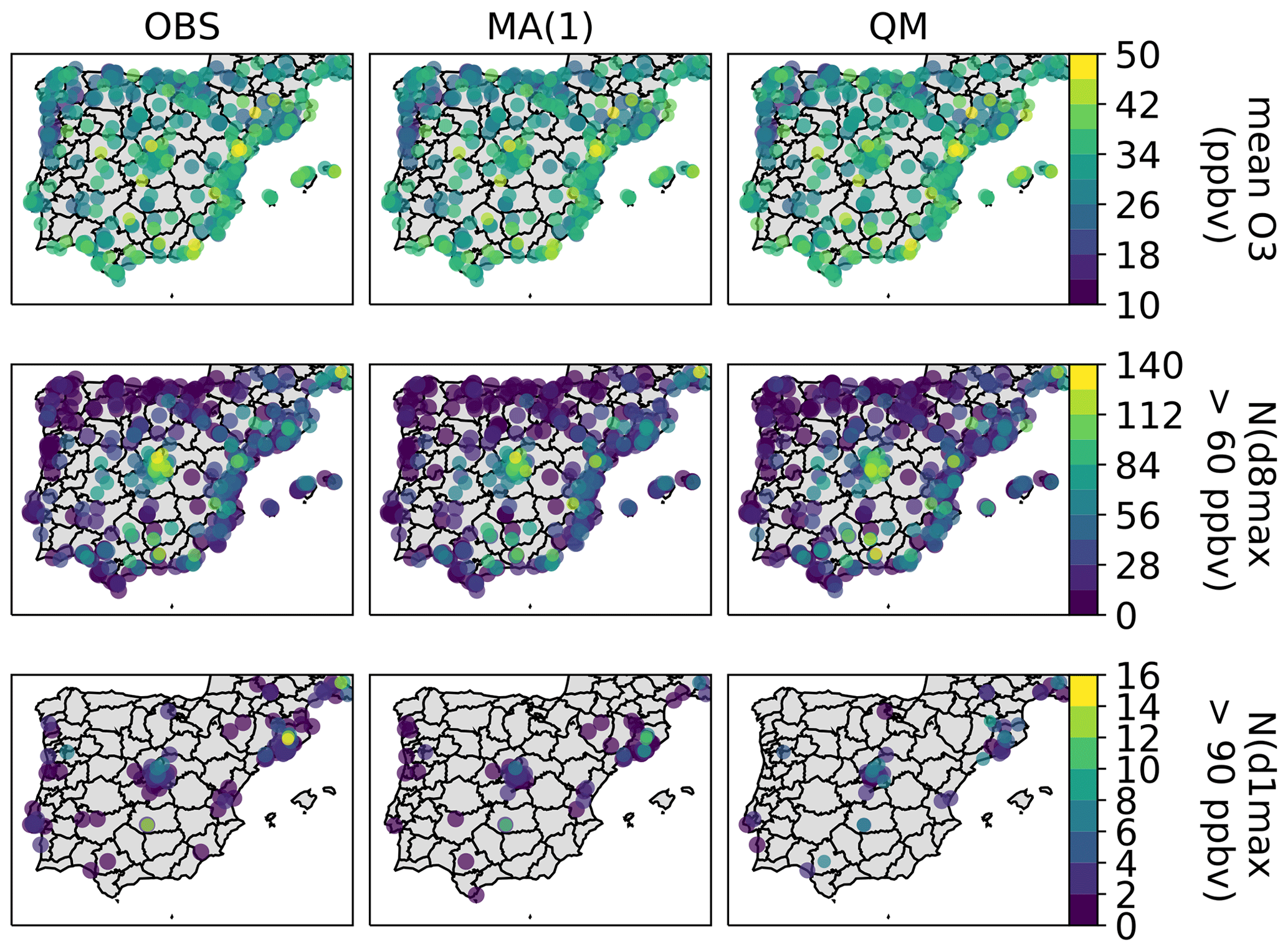
Figure 5Similar to Fig. 1 but for observations and D+4 O3 forecasts corrected with MA(1) and QM methods.
Table 2Evaluation of the different forecast methods on categorical metrics, at D+1 (and D+4 in parentheses), for both target and information thresholds.
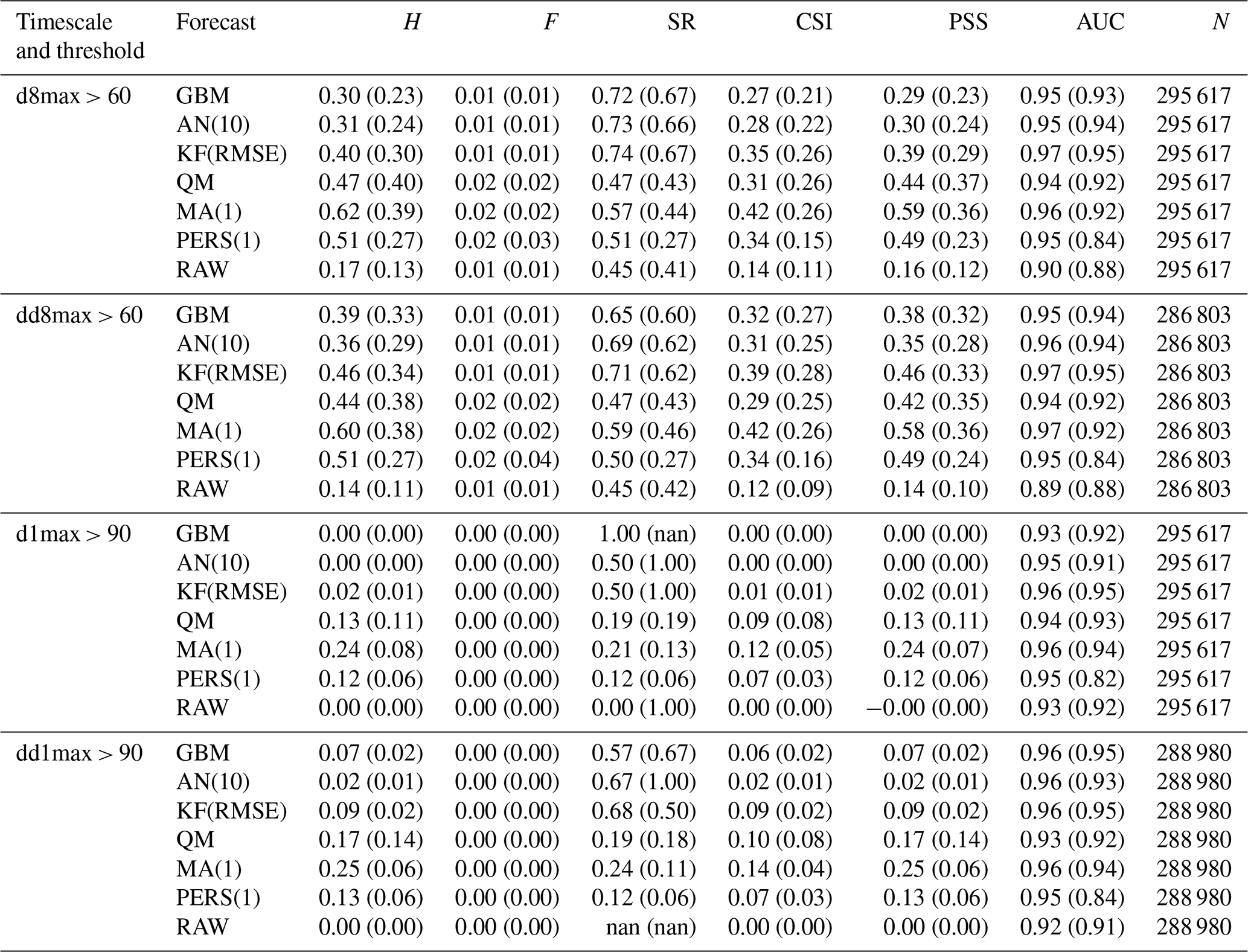
nan: not a number.
3.4 Sensitivity tests
Each of the forecast methods considered in this study relies on a specific configuration, e.g., the time window of PERS or MA methods, the metric used internally in KF for optimizing the variance ratio, the number of analogs taken into account in AN, the choice of input features, or metrics used internally for fitting the ML model in GBM. This configuration can substantially influence their general performance, although in a different way depending on the metric used. In the previous sections, we evaluated the performance of these different methods considering a relatively simple baseline configuration. In this section, we discuss some of these choices and investigate their impact on the performance through different sensitivity tests. Corresponding statistical results on continuous and categorical metrics are given in the tables in the Supplement.
3.4.1 Persistence method
The persistence method with a 1 d time window (PERS(1)) provides a reference forecast for assessing the skill scores on the different RAW and MOS-corrected forecasts. Here we explore how the time window, from 1 to 10 d (hereafter referred to as PERS(n), with n the window in days), impacts the performance of this PERS forecast. Results are shown in Fig. G1 in Appendix G.
Increasing the window leads to a growing negative bias on d1max and d8max scales that can be substantially reduced when working at dd1max and dd8max scales, i.e., when applying the PERS approach directly on daily 1 and 8 h maxima rather than on the hourly time series. The differences between the two approaches originate from the day-to-day variability in the hour of the day when O3 mixing ratios peak. For illustration purposes, let us assume that O3 peaks between 15 and 17 h; on a given day, O3 mixing ratios at 15, 16 and 17 h reach 50, 60 and 50 ppbv and on the following day 70, 70 and 80 ppbv. Then, the PERS(2)dd1max O3 would be 70 ppbv (mean of 60 and 80 ppbv), while the PERS(2)d1max O3 would be only 65 ppbv (maximum of the mean diurnal profile of these 2 d, in this case 60, 65 and 65 ppbv). Conversely, both nRMSE and PCC can be slightly improved with longer windows, but at the cost of a growing underestimation of the variability. As a consequence, both H and F are slightly reduced, which means that PERS forecasts become more “conservative” with longer windows. The impact on SR for detecting exceedances of the target threshold is low for short lead times but positive for the longest ones. Interestingly, for information thresholds, the best SRs are obtained around 4–7 d. However and more importantly, using longer windows deteriorates the general performance of the forecast, as shown by the decrease in both CSI and PSS, especially at short lead times. Interestingly, there are also important differences in terms of AUC for detecting exceedances of the target threshold depending on the lead day, ranging from a decrease in AUC with longer windows at D+1 to an increase at D+4.
Therefore, for detecting exceedances, considering PSS and/or CSI as the most relevant metrics, the PERS method shows its best performance for a time window of 1 d. However, it gives very “liberal” O3 forecasts with rather poor SR. The term “liberal” is borrowed here from Fawcett (2006) to designate forecasting systems that predict exceedances with weak evidence, in opposition with the aforementioned term “conservative”. Longer time windows can improve SR but result in an important deterioration of CSI and PSS, particularly for the shorter lead times (D+1 and D+2).
3.4.2 Moving average method
Here, a sensitivity test is performed on MA with windows ranging between 1 and 10 d (hereafter referred to as MA(n), with n the window in days). Results are shown in Fig. G2 in Appendix G. Increasing the window length impacts the MA performance in a very similar way to PERS, especially for continuous metrics. Regarding the detection of the target threshold, the main noticeable difference is the absence of strong deterioration of some metrics like AUC, SR or CSI for shorter lead times. Regarding the detection of the information threshold, the clearest difference with PERS concerns the SR that substantially improves when considering longer windows. However, the deterioration of both CSI and PSS persists.
Therefore, the detection of O3 exceedances with the MA method shows its best performance with the shortest windows (1 d). As for PERS, the corresponding forecasts are quite liberal with low SR. However, in contrast to PERS, the SR associated with high thresholds can be substantially improved when using longer windows, which may be an interesting option if the corresponding deterioration of CSI and PSS is seen as acceptable.
3.4.3 Kalman filter method
As explained in Sect. 2.3.3 (and Appendix B), the behavior of the KF intrinsically depends on the ratio chosen. So far, this parameter has been adjusted dynamically (and updated regularly) to optimize the RMSE of past data. Here, a sensitivity test is performed with alternative strategies in which the variance ratio is chosen to optimize the SR, CSI, PSS or AUC with threshold values of 60 or 90 ppbv (hereafter referred to as SR-60, SR-90, CSI-60, CSI-90, PSS-60, PSS-90, AUC-60 and AUC-90). The objective is to investigate the extent to which tuning the KF algorithm with appropriate categorical metrics allows improving the exceedance detection skills.
Results (Fig. G3 in Appendix G) show that this tuning strategy barely impacts the performance obtained on continuous metrics, except for CSI-60 and PSS-60 that show slightly deteriorated RMSE and PCC. Only small differences are also found on target threshold exceedances, except again with these two methods that show slightly improved CSI and PSS at short lead time. Results on information threshold exceedances show more variability depending on the timescale, but both CSI and PSS can typically be improved when used internally in the KF procedure, although often only at short lead times. The choice of the threshold in this optimizing metric leads to more ambiguous results. For instance, besides giving the best PSS on the target threshold, KF(PSS-60) also gives better results than KF(PSS-90) on the information threshold. Reasons behind this behavior are not clear but may be due to some instabilities brought into PSS-90 by the rareness of such exceedances. Indeed, a common and well-known issue of PSS (as well as CSI and most other categorical metrics) is that it degenerates to trivial values (either 0 or 1) for rare events: as the frequency of the event decreases, the numbers of hits (a), false alarms (b) and missed exceedances (c) all decay toward zero but typically at different rates, which causes the metric to take meaningless values (either 0 or 1 in the case of PSS) (Jolliffe and Stephenson, 2011; Ferro and Stephenson, 2011). All in all, the performance for detecting such high O3 concentrations remains very poor, especially far in time, but this sensitivity test demonstrates that choosing an appropriate tuning strategy can help to slightly improve the detection skills at a potential cost in terms of continuous metrics.
3.4.4 Analog method
The AN method identifies the closest analog days to estimate the corresponding prediction and thus depends on the number of analog days taken into account. We performed a sensitivity test with 1, 5, 10, 15, 20, 25 and 30 analog days (hereafter referred to as AN(N), with N the number of analogs). Results are shown in Fig. G4 in Appendix G.
Although the best slopes are found with the smallest number of analogs, the best nRMSE and PCC are obtained using around 5–15 analogs. Using too many analogs increases the underestimation of the variability and deteriorates the slope. Regarding the detection of target thresholds, increasing the number of analogs makes the forecast more “conservative” (lower H and F, higher SR) and deteriorates the CSI and PSS. When focusing on information threshold exceedances, the AN forecasts based on 10 analogs or more never reach such high O3 values. The highest CSI and PSS are finally obtained with one single analog.
Therefore, similarly to PERS and MA methods that reached their best skills for the shortest time windows, with AN the best CSI and PSS skills are obtained when using the lowest number of analogs (with a cost in the continuous metrics, as for PERS and MA). Computing the AN-corrected O3 mixing ratios based on a larger number of analogs gives smoother predictions, and our choice to weight the average by the distance to the different analogs is unable to substantially mitigate this issue.
3.4.5 Gradient boosting machine method
Although GBM gives among the best RMSE and PCC, it strongly underestimates the variability in O3 mixing ratios, with critical consequences in terms of detection skills, especially for the highest thresholds (e.g., d1max > 90 ppbv). This is at least partly due to the low frequency of occurrence of such episodes and their corresponding low weight in the entire population of points used for the training. One way of mitigating this issue consists of specifying different weights to the different training instances. This aims at forcing the GBM model to better predict the instances of higher weight, at the cost of a potential deterioration of the performance on the instances of lower weight.
In order to assess the extent to which it may improve the performance of the GBM MOS method, we test here different weighting strategies. At each training phase, we compute the absolute distance D between all observed O3 mixing ratio instances and the mean O3 mixing ratio (averaged over the entire training dataset). Then several sensitivity tests are performed, weighting the training data by D, D2 and D3, respectively (hereafter referred to as GBM(W), GBM(W2) and GBM(W3), respectively). Using such weights, we want the GBM model to better predict the lower and upper tails of the O3 distribution in order to better represent the variability in the O3 mixing ratios. Given that the O3 mixing ratio distribution is typically positively skewed, the highest weights are put on the strongest positive deviations from the mean.
As a parallel sensitivity test, we explore the performance of these different ML models but remove the input feature corresponding to the previous (1 d before) observed O3 mixing ratio (hereafter referred to as GBM(noO), GBM(noO,W), GBM(noO,W2) and GBM(noO,W3)). This additional test is of interest for operational purposes since O3 observations are not always available in near real time. Results are shown in Fig. G5 in Appendix G.
As expected, the results highlight a deterioration of the RMSE and PCC combined with an improvement in the slope and nMSDB. The negative bias affecting the variability with the unweighted GBM is substantially reduced when using weights, although too-strong weights (as in GBM(W3) for instance) can lead to a slight overestimation of the variability at specific timescales.
Regarding the skills for detecting target threshold exceedances, stronger weights typically increase both H and F and improve the (underestimated) FB but deteriorate the SR and AUC (the forecasts become more liberal). Regarding the more balanced metrics (of strongest interest here), adding more weights on the tails of the O3 distribution typically has a positive although small impact on CSI and PSS. Regarding the detection of information threshold exceedances, both CSI and PSS can also be slightly improved by adding some weight into the GBM, but the performance for detecting such high O3 values remains relatively low. The interest of using the O3 concentration observed 1 d before is found here to be limited.
Therefore, adopting an appropriate weighting strategy is simple yet effective for achieving slightly better O3 exceedance detection skills in exchange for a reasonable deterioration in RMSE and PCC. Overall, the improvements are relatively small, but still valuable given the initially very low detection skills for the strongest O3 episodes.
3.4.6 Influence of the meteorological input data in AN and GBM methods
In the previous sections, O3 corrections with AN and GBM methods relied on HRES meteorological forecasts. Here, we investigate the impact of using alternative meteorological data, namely the ERA5 meteorological reanalysis. For both AN and GBM methods, the MOS-corrected O3 mixing ratios obtained with these two meteorological datasets are very similar, with PCC above 0.95. The results obtained against observations are shown in Fig. G6 in Appendix G, for the AN(1), AN(5), AN(10) and GBM methods. Since O3 predictions are close, the statistical performance against observations is also very consistent between both meteorological datasets. For both continuous and categorical metrics, the performance obtained with HRES data is found to be slightly lower than with ERA5. Discrepancies between both meteorological datasets tend to increase with lead time, with GBM being slightly more sensitive to the meteorological input data than AN.
Therefore, this experiment highlights a relatively low sensitivity of both AN and GBM methods to the two meteorological datasets tested here. The very similar results obtained with IFS and ERA5 meteorological input data are likely not explained by the fact that both datasets give very similar values for the different meteorological variables, but rather by the intrinsic characteristics of both AN and GBM methods. The AN method makes use of the meteorological data only to identify past days with more or less similar meteorological conditions and can thus handle to some extent the presence of biases in meteorological variables as far as they are systematic (and thus do not impact the identification of the analogs). On the other hand, the GBM method uses past information to learn the complex relationship between O3 mixing ratios and the other ancillary features. Although the better the input data, the higher the chances are to fit a reliable model for predicting O3, the GBM models can also indirectly learn at least part of the potential errors affecting some meteorological variables and how they relate to O3 mixing ratios. Therefore, the presence of biases in some of the ancillary features is not expected to strongly impact the performance of the predictions.
We demonstrated the strong impact of MOS methods to enhance raw CAMS O3 forecasts, not only by removing potential systematic biases but also by correcting other issues related to the distribution of and/or variability in O3 mixing ratios. All MOS approaches were indeed able to substantially improve at least some aspects of the RAW O3 forecasts, first and foremost the RMSE and PCC, for which the strongest improvements are obtained with the most sophisticated MOS methods like KF, AN or GBM. However, although all MOS methods were able to increase the underestimated variability in O3 mixing ratios of RAW, the strongest improvements in slope and nMSDB were obtained with more simple MOS methods like MA or QM. O3 mixing ratios corrected with AN, GBM and to a lesser extent KF remained too smooth, and such a deficiency has a major impact on the detection skills for high O3 thresholds. All in all, the best PSS and CSI are usually obtained with the more simple MOS methods. Therefore, there is a clear trade-off between the continuous and categorical skills scores, as also shown by the different sensitivity tests. The quality of a MOS-corrected forecast assessed solely based on metrics like RMSE or PCC thus tells little about the forecast value, here understood as information a user can benefit from to make better decisions, notably for mitigating O3 short-term episodes.
More generally, our study highlights the complexity of identifying the “best” MOS method given the multiple dimensions of the problem. The relative performance of the MOS methods can vary depending on the metric used, the threshold considered in the case of categorical metrics (or more specifically the base rate), the timescale at which MOS corrections are computed and/or evaluated, or the lead time. Other dimensions not covered by this study, like the seasonality of the performance, are also susceptible to shedding a different light on the intercomparison.
Among the continuous metrics, both RMSE and PCC provide initial valuable information on the performance of a MOS method. However, a MOS method can give the best RMSE and PCC, yet the poorest high O3 detection skills. This was the case of the unweighted GBM method. Continuous metrics like the model-versus-observation linear slope or nMSDB provide important complementary information, potentially less misleading, especially in a context where the final objective is to predict episodes of strong O3. Among the categorical metrics, although results were presented on a relatively large set of metrics, not all metrics benefit from the same properties. PSS may be considered to be one of the most valuable, notably due to its independence from the base rate, in contrast to CSI. Such a property is particularly useful when comparing scores over different regions and/or time periods where the frequency of observed exceedances might vary, for instance due to different emission forcing and/or meteorological conditions. In an operational context where statistical metrics are continuously monitored, the independence from the base rate is an interesting property because it may change with time, which prevents a consistent comparison between different periods. However, a well-known issue of both PSS and CSI (as well as many other categorical metrics) is that they degenerate to trivial values (either 0 or 1) as events become rarer (Jolliffe and Stephenson, 2011; Ferro and Stephenson, 2011), which should restrict their use to the detection of not-too-rare (and therefore not-too-high) O3 episodes. In this study, the base rate of the target threshold was likely sufficiently high (s around 5 %), but we were probably already at the limit regarding the information threshold (s around 0.1 %). All in all, the selection of the evaluation metrics depends on the subjective choices and intended use and is fundamentally a cost–loss problem where the user should arbitrate between the cost of missing exceedances and predicting false alarms.
The performance of the RAW forecasts was found to be only slightly sensitive to the lead day, but this sensitivity was substantially stronger with some MOS methods (although lower than for the persistence method). This aspect is important, although different users may have different needs in terms of lead time, depending on the intended use of the AQ forecast. Forecasts at D+1 may already be useful for some applications like warning the vulnerable population in advance so that they could adapt their outdoor activities. However, implementing short-term emission reduction measures at the local scale usually goes through decisions taken at different administrative and political levels and thus typically requires forecasts at least at D+2. If such measures would have to be taken at a larger scale, the occurrence of O3 episodes would probably need to be forecasted even more in advance.
We saw that some forecast methods like PERS or MA can provide a reasonable performance at D+1 but quickly deteriorate when looking further in the future (while other methods like GBM, AN or QM were less impacted by the lead time). Actually, the performance of our PERS(1) reference forecast obviously depends on the typical duration of O3 episodes over the region of study; one (single) episode is defined here as a suite of successive days showing an exceedance of a given threshold at a given station. Over the Iberian Peninsula domain in 2018–2019, considering the target threshold (d8max > 60 ppbv), a total of 6540 such O3 episodes were observed in the O3 monitoring network with min, mean and max duration of 1, 2 and 27 d (and 5th, 25th, 50th, 75th and 95th percentiles of 1.0, 1.0, 1.0, 2.0 and 5.0 d). Note the 27 d long O3 exceedance occurred in June–July 2019 about 30 km north of Madrid (station code ES1802A). Considering the information threshold, 240 episodes were observed, with min, mean and max duration of 1, 1.1 and 5 d (and 5th, 25th, 50th, 75th and 95th percentiles of 1.0, 1.0, 1.0, 1.0 and 2.0 d). This may partly explain why the deterioration of performance with lead time was stronger for target thresholds compared to information thresholds.
For operational purposes, several important aspects are to be taken into account. A first aspect concerns the input data required by the MOS method. Does the MOS method rely on observations, models or a combination of both? When the method relies on observations, are they needed in near real time? How many historical data are required? When the method relies on historical data, to which extent does the length of the historical dataset impact the performance? Related to this last point, another essential aspect concerns the ability of the MOS method to handle progressive and/or abrupt changes in the AQ forecasting system (e.g., configuration, parameterizations, input data like emissions) and/or in the Earth's atmosphere (long-term trends, anomalous events like the COVID-19-related emission reduction, climate change). In this framework, the year 2020 obviously offers a unique large-scale case study to investigate the behavior of the different MOS methods.
MOS methods relying only on very recent data (namely MA and KF methods) are evidently more adaptable to rapid changes, which is a clear asset under changing atmospheric conditions or modeling system configurations. On the other hand, they naturally discard all the potentially useful information available within the historical dataset. Methods like QM, AN or GBM aim at extracting such information to produce better forecasts but implicitly rely on the assumption that these historical data are still up to date and thus representative of the current conditions, which can be too strong a hypothesis when the historical dataset is long, or the emission forcing and/or meteorological conditions are changing rapidly. In this study, we considered a relatively short 2-year dataset, but using a longer training dataset would likely require building specific methodologies to tackle this issue, either by identifying and discarding the potentially outdated data or by giving them a lower weight in the procedure.
In this study, we implemented a relatively simple ML-based MOS method. Although the performance on categorical metrics was found to be limited despite encouraging results on continuous metrics, there is likely room for improvements in near-future developments. In order to improve the high O3 detection skills, potential interesting aspects to explore include testing other types of ML models, customizing loss function and/or cross-validation scores, designing specific weighting strategies and/or re-sampling approaches, or comparing regression and classification ML models for the detection of exceedances. Along the preparation of this study, some of them have been investigated, but more efforts are required to draw firm conclusions regarding their potential for better predicting O3 episodes. Finally, we focused here on the CAMS regional ensemble, but including the individual CAMS models in the set of ML input features may help to achieve better performance if the ML model is somehow able to learn the variability (in time and space or during specific meteorological conditions) in strengths and weaknesses of each model and build its predictions based on the most appropriate subset of individual models. More generally, the performance of the different MOS methods is expected to vary from one raw model to another. Investigating the performance and behavior of these methods on the different individual models might shed an interesting light on the results obtained here with the ensemble and eventually allow some of our conclusions to be generalized.
Using the metadata available in GHOST (Globally Harmonised Observational Surface Treatment), a quality assurance screening is applied to O3 hourly observations, in which the following data are removed: missing measurements (GHOST's flag 0), infinite values (flag 1), negative measurements (flag 2), zero measurements (flag 4), measurements associated with data quality flags given by the data provider which have been decreed by the GHOST project architects to suggest the measurements are associated with substantial uncertainty or bias (flag 6), measurements for which no valid data remain to average in temporal window after screening by key QA flags (flag 8), measurements showing persistently recurring values (rolling seven out of nine data points; flag 10), concentrations greater than a scientifically feasible limit (above 5000 ppbv) (flag 12), measurements detected as distributional outliers using adjusted boxplot analysis (flag 13), measurements manually flagged as too extreme (flag 14), data with too coarse reported measurement resolution (above 1.0 ppbv) (flag 17), data with too coarse empirically derived measurement resolution (above 1.0 ppbv) (flag 18), measurements below the reported lower limit of detection (flag 22), measurements above the reported upper limit of detection (flag 25), measurements with inappropriate primary sampling for preparing NO2 for subsequent measurement (flag 40), measurements with inappropriate sample preparation for preparing NO2 for subsequent measurement (flag 41) and measurements with erroneous measurement methodology (flag 42).
In this section, we briefly describe the application of the Kalman filter as a MOS correction method. More details can be found for instance in Delle Monache et al. (2006), while Pei et al. (2017) provide a clear general introduction to the Kalman filter. CAMS forecasts are available over 4 lead days, from D+1 to D+4. We define here the time t as the day D at a given hour of the day (t+1 thus corresponds to D+1 at this specific hour of the day). In an operational context, observations at this hour of the day are available only until time t (included). In this framework, our primary objective in this MOS approach is to estimate , the true (unknown) forecast bias at time t+1 using the information available until t (included), which can then be used to correct the raw CAMS forecast. Here, can be referred to as the a priori forecast bias at time t+1, while can be referred to as the a posteriori forecast bias at time t+1 as it takes advantage from the information obtained at t+1. We distinguish estimated values from true values using a hat ( ) ( therefore corresponds to the estimated value of ). In its application as a MOS method, the Kalman filter considers the following process equations for describing the time evolution of the forecast bias:
where ηt+1 represents the process noise and is assumed to be a white noise term with normal distribution, zero mean, variance and uncorrelated in time, and is the a priori expected error variance of the forecast bias estimate. Our process equations here are thus quite simple as we assume that the a priori forecast bias at time t+1, , is similar to the previous a posteriori forecast bias xt|t but with some uncertainty ηt+1.
At time t+1, an observation of the forecast bias xt+1, denoted zt+1, is available but with some uncertainty (since the measurement of the pollutant concentration necessarily comes with some uncertainty):
where ϵt+1 represents the measurement noise and is assumed to be a white noise term with normal distribution, zero mean, variance , uncorrelated in time and independent of the process noise ηt+1. Then, the Kalman filter allows this observation zt+1 and the a priori estimate of the forecast bias to be fused in order to obtain an a posteriori estimate of the forecast bias :
where Kt+1 corresponds to the so-called Kalman gain used to weight the respective importance of the a priori forecast bias estimate () and its observed value (zt+1), and corresponds to the expected error in the forecast bias estimate (i.e., the variance of the forecast bias error: ).
In practice, the KF algorithm first requires initialization of the and p0|0 values (any reasonable value can be chosen, given that the KF quickly converges). Then the algorithm starts its first iteration. As a first step, the a-priori-estimated value of the forecast bias is obtained from (in our problem, we simply have ) and used to correct the raw forecast of CAMS. As a second step, after obtaining the observed pollutant concentration, one can deduce z1 and fuse it with using the Kalman filter equations, which gives us the a-posteriori-estimated value of the forecast bias that will be available for the second iteration. An overview of this workflow is given in Fig. B1.

Solving these equations requires values to be assigned to both variances and . It can be demonstrated that, once is set to a fixed value (any reasonable value can be chosen, for instance ), the KF results mainly depend on the variance ratio. Various strategies can be used to choose an appropriate value for this variance ratio. This aspect is discussed in Sect. 2.3.3.
The analogs (AN) method requires identification of which past forecast days are the most similar to the current one. Given a set of features to take into account, this similarity is computed using the norm introduced by Delle Monache et al. (2006):
with Ft the raw forecast at time t, an analog forecast at time t′, N the number of features taken into account, wi the weight of the feature i, σi its standard deviation calculated over past forecasts and T the half-width of the time window over which to compute the metric (i.e., a value T=2 means that the squared difference between the forecast and the analog will be computed over a ±2 h time window). In our study, we used weights of 1 for all features (wind speed, wind direction, temperature, surface pressure) and T=1.
The GBM models are tuned using a so-called randomized search in which a range of values is given for each hyperparameter of interest and a total number of hyperparameters combinations to test. After fixing the learning rate to 0.05 (learning_rate in the scikit-learn Python package), the tuning of the GBM model was done over the following set of hyperparameters: the tree maximum depth (max_depth: from 1 to 5 by 1), the subsample (subsample: from 0.3 to 1.0 by 0.1), the number of trees (n_estimators: from 50 to 1000 by 50) and the minimum number of samples required to be at a leaf node (min_samples_leaf: from 1 to 50). As we are dealing here with time series, this tuning is conducted through a rolling-origin cross-validation in which validation data are always posterior to train data.
The continuous metrics used in this study are defined as follows:
with mi and oi the predicted and observed mixing ratios, and their corresponding mean, σm and σm their corresponding standard deviation, and N the number of points.
The performance of the categorical forecasts of exceedances beyond a certain threshold can primarily be described through a contingency table (Table E1). Based on these individual numbers a (hits), b (false alarms), c (misses) and d (correct rejections), a wide number of verification metrics have been proposed in the literature, often with inconsistent nomenclature. In order to avoid confusion, all metrics used in this paper systematically follow the nomenclature given in the reference book of Jolliffe and Stephenson (2011).
For a given total number of data n (), the 2×2 contingency table can be fully described by three independent measures, namely the base rate s independent of the forecasting system (total proportion of observed exceedances, also known as the climatological probability of an exceedance), the hit rate H (proportion of the observed exceedances that are correctly detected) and the false alarm rate F (proportion of the observed non-exceedances erroneously forecast as exceedances, to be distinguished from the false alarm ratio). These metrics as well as the other categorical metrics used in this study – frequency bias (FB), success ratio (SR), critical success index (CSI) or Peirce skill score (PSS) – are defined as follows:
Note that as shown in these formulas, any categorical metric that is initially a function of a, b, c and d can be expressed in terms of s, H and F. One interest of considering this s–H–F framework (so-called likelihood–base rate factorization; see chapter 3 of Jolliffe and Stephenson, 2011, for a detailed description) lies in the fact that, since the forecaster does not have any influence on s, the tri-dimensional problem is reduced to a bi-dimensional problem (H and F). Since it is easily possible to maximize H (by always predicting an exceedance) or F (by always predicting a non-exceedance), none of these two metrics taken individually is a good and balanced metric for assessing the quality of a forecasting system; only some combinations of both (possibly with s) can eventually provide a good way to assess these detection skills, such as those used in this study.
Table E1Schematic contingency table for deterministic forecasts of binary exceedances of the regulatory limit values.

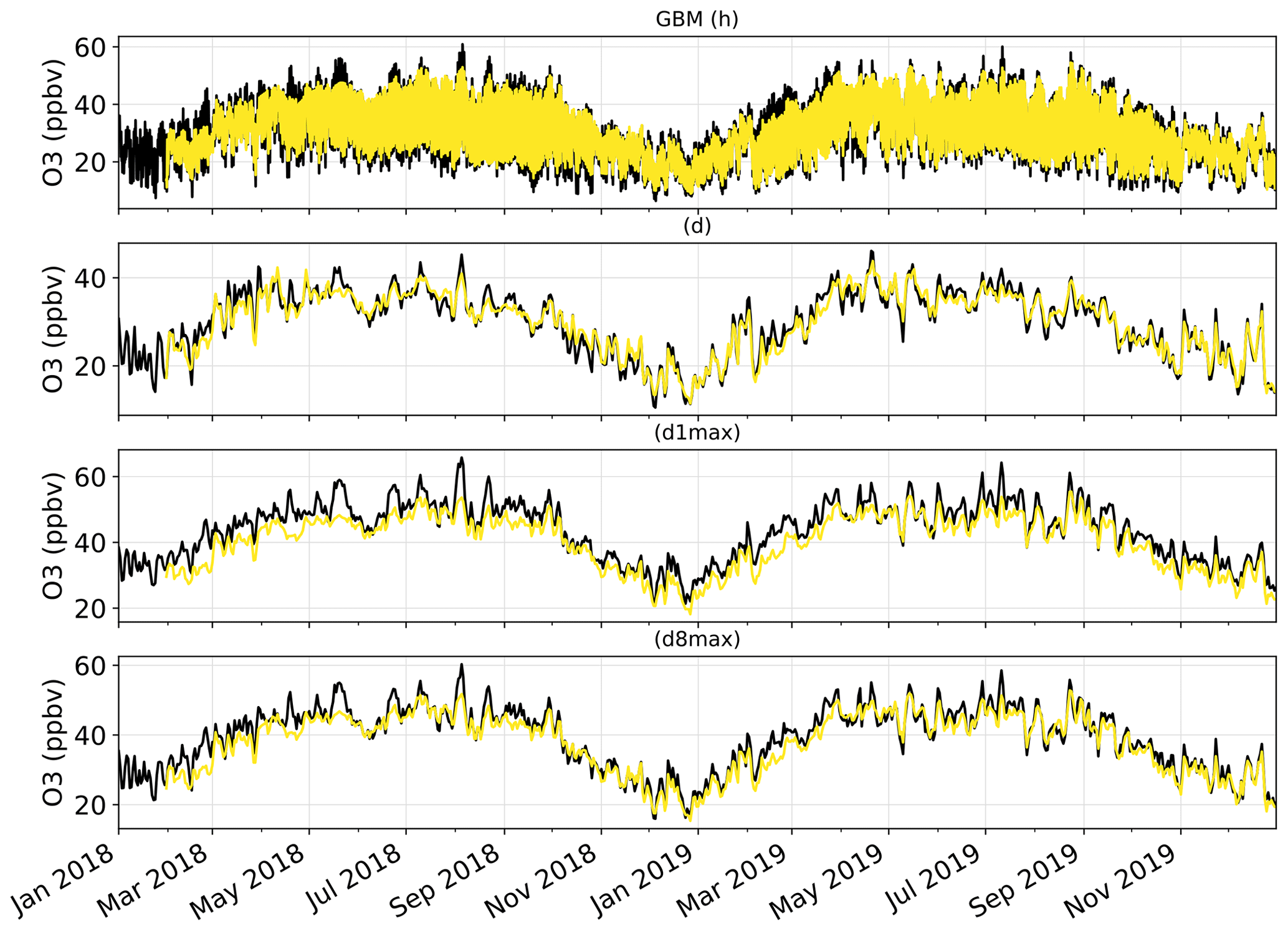
Figure F1Time series of the mean O3 mixing ratios over the Iberian Peninsula, as observed by monitoring stations (in black) and as simulated by CAMS D+1 forecasts corrected with the GBM MOS method (in yellow). Time series are shown at the hourly (h), daily mean (d), daily 1 h maximum (d1max) and daily 8 h maximum (d8max) timescales. O3 mixing ratios are averaged over all surface stations of the domain.
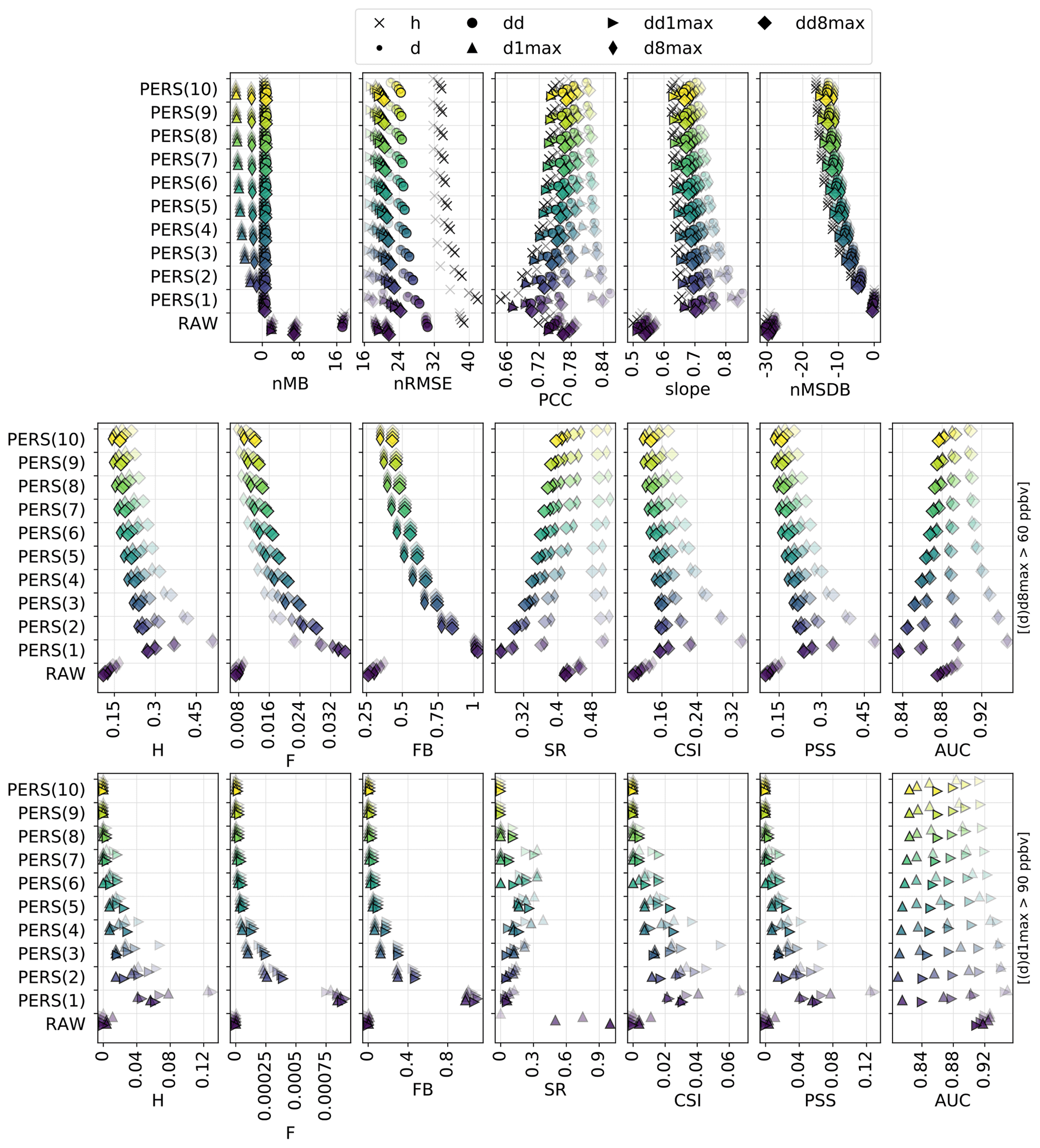
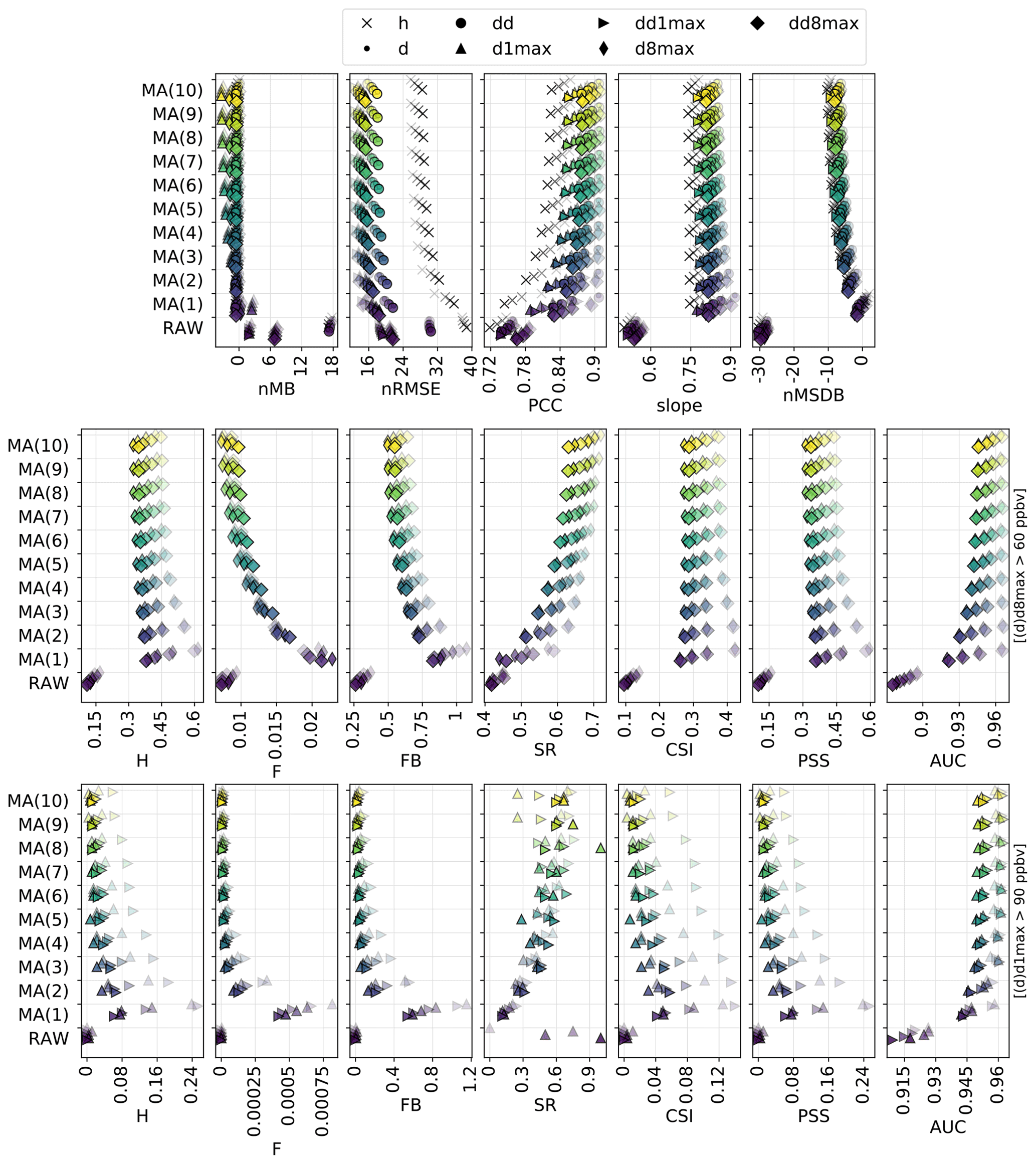
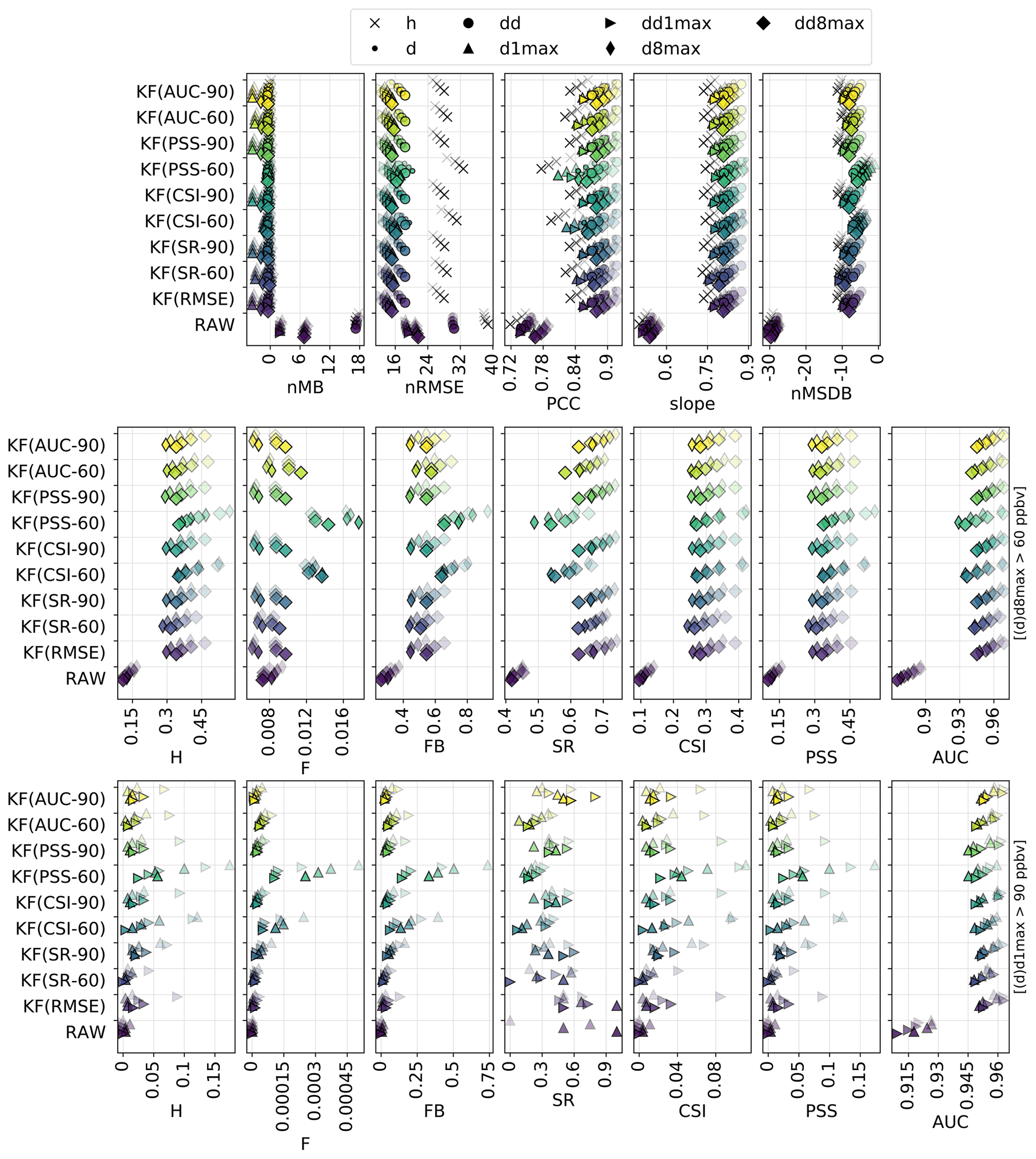
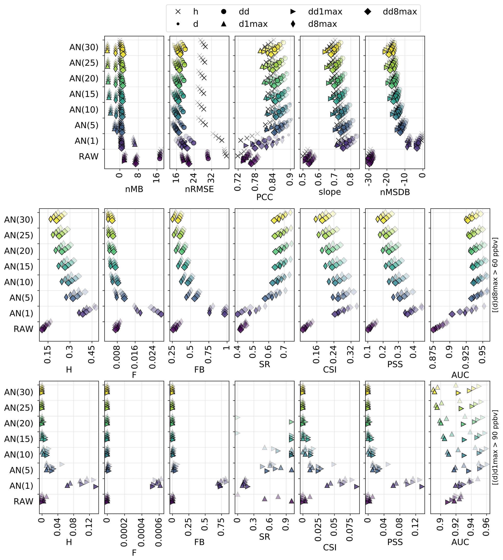
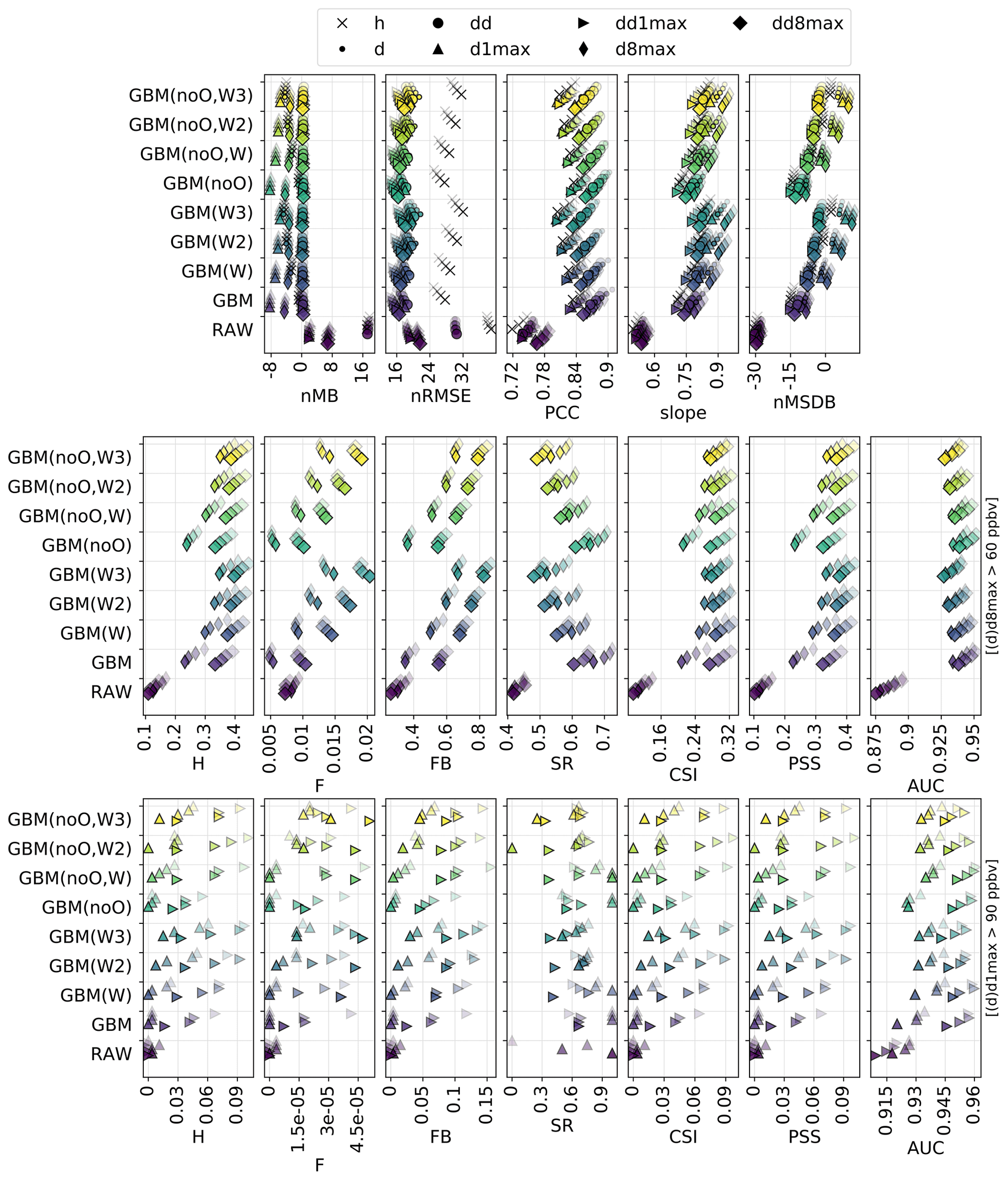
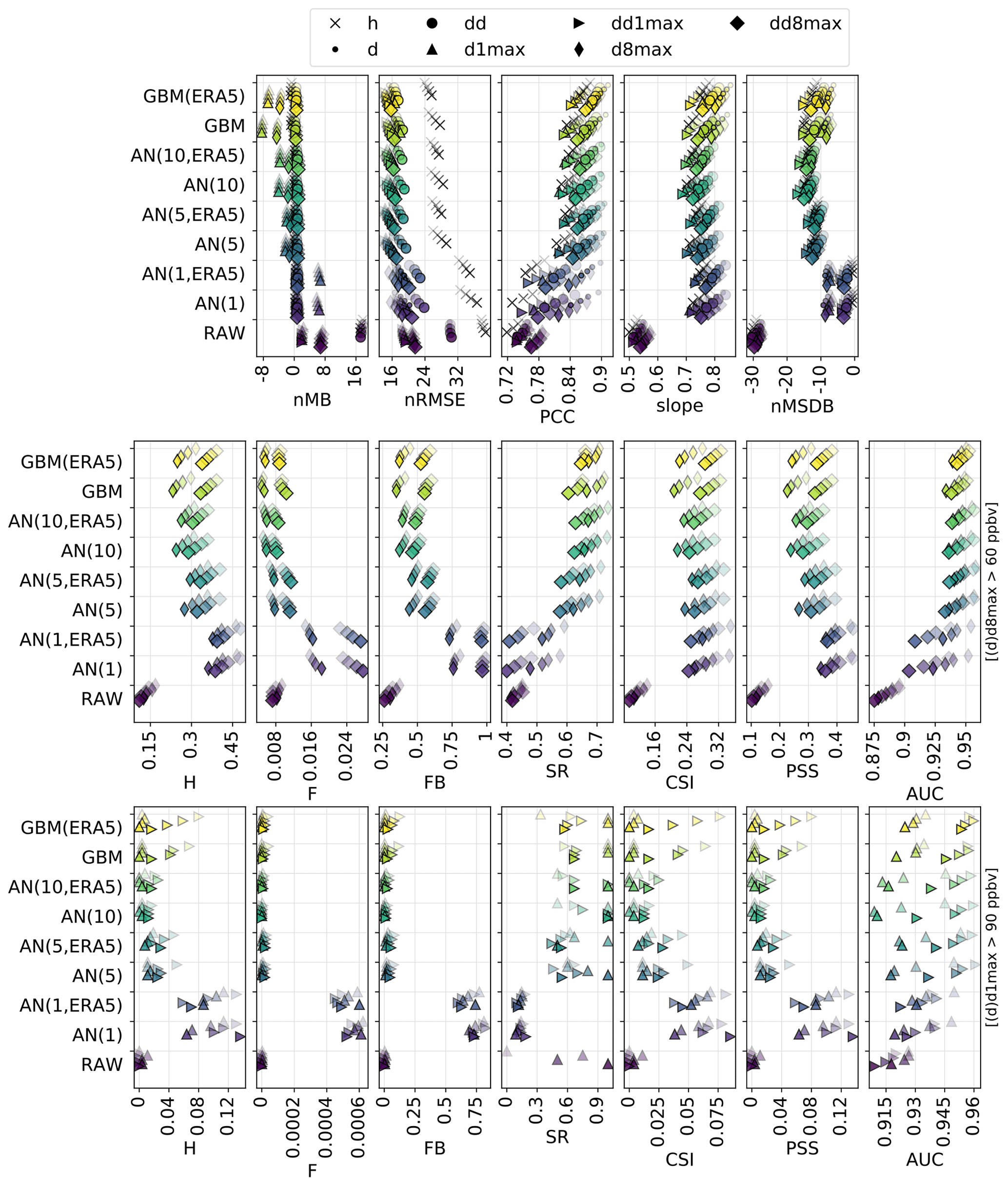
The EEA AQ e-Reporting dataset is publicly available (https://www.eea.europa.eu/data-and-maps/data/aqereporting-2; EEA, 2021), as well as the ERA5 meteorological dataset (https://doi.org/10.24381/cds.adbb2d47; Hersbach et al., 2018) and the CAMS regional forecasts (https://atmosphere.copernicus.eu/catalogue#/; Copernicus, 2020).
The supplement related to this article is available online at https://doi.org/10.5194/acp-22-11603-2022-supplement.
HP contributed to the conception and design of the study. PAB and MSC were responsible for downloading the CAMS and meteorological data. KS was responsible for installing the Python packages and other useful modules on the MareNostrum supercomputer. DB was responsible for the acquisition and preprocessing of the air quality data through the GHOST project. HP carried out the analysis. HP, CPGP, OJ, AS, MG, JMA and DB contributed to the interpretation of results. HP was responsible for writing the article, with a careful review from CPGP and JAM.
The contact author has declared that none of the authors has any competing interests.
Publisher’s note: Copernicus Publications remains neutral with regard to jurisdictional claims in published maps and institutional affiliations.
This research has been funded by the European Union's Horizon 2020 research and innovation program under the Marie Skłodowska-Curie grant agreement H2020-MSCA-COFUND-2016-754433, as well as the MITIGATE project (PID2020-113840RA-I00 funded by MCIN/AEI/10.13039/501100011033) from the Agencia Estatal de Investigacion (AEI). We also acknowledge support by the AXA Research Fund and Red Temática ACTRIS España (CGL2017-90884-REDT), the BSC-CNS “Centro de Excelencia Severo Ochoa 2015-2019” program (SEV-2015-0493), PRACE, and RES for awarding us access to the MareNostrum supercomputer in the Barcelona Supercomputing Center as well as H2020 ACTRIS IMP (no. 871115). We also acknowledge support from the VITALISE project (PID2019-108086RA-I00) funded by MCIN/AEI/10.13039/501100011033.
This research has been supported by the Agencia Estatal de Investigación (MITIGATE project, grant no. PID2020-113840RA-I00 funded by MCIN/AEI/10.13039/501100011033) and the H2020 Marie Skłodowska-Curie Actions (grant no. H2020-MSCA-COFUND-2016-754433).
This paper was edited by Pedro Jimenez-Guerrero and reviewed by three anonymous referees.
Borrego, C., Monteiro, A., Pay, M., Ribeiro, I., Miranda, A., Basart, S., and Baldasano, J.: How bias-correction can improve air quality forecasts over Portugal, Atmos. Environ., 45, 6629–6641, https://doi.org/10.1016/j.atmosenv.2011.09.006, 2011. a
Bowdalo, D.: Globally Harmonised Observational Surface Treatment: Database of global surface gas observations, in preparation, 2022. a
Caruana, R. and Niculescu-Mizil, A.: An empirical comparison of supervised learning algorithms using different performance metrics, Tech. rep., Technical Report TR2005-1973, Cornell University, 2005. a
Copernicus: Catalogue, Copernicus [data set], https://atmosphere.copernicus.eu/catalogue#/, last access: 20 November 2020. a
Copernicus Climate Change Service (C3S): ERA5: Fifth generation of ECMWF atmospheric reanalyses of the global climate, 2017. a
De Ridder, K., Kumar, U., Lauwaet, D., Blyth, L., and Lefebvre, W.: Kalman filter-based air quality forecast adjustment, Atmos. Environ., 50, 381–384, https://doi.org/10.1016/j.atmosenv.2012.01.032, 2012. a
Delle Monache, L., Nipen, T., Deng, X., Zhou, Y., and Stull, R.: Ozone ensemble forecasts: 2. A Kalman filter predictor bias correction, J. Geophys. Res., 111, D05308, https://doi.org/10.1029/2005JD006311, 2006. a, b, c, d
Delle Monache, L., Nipen, T., Liu, Y., Roux, G., and Stull, R.: Kalman Filter and Analog Schemes to Postprocess Numerical Weather Predictions, Mon. Weather Rev., 139, 3554–3570, https://doi.org/10.1175/2011MWR3653.1, 2011. a, b, c
Delle Monache, L., Eckel, F. A., Rife, D. L., Nagarajan, B., and Searight, K.: Probabilistic Weather Prediction with an Analog Ensemble, Mon. Weather Rev., 141, 3498–3516, https://doi.org/10.1175/MWR-D-12-00281.1, 2013. a
Di Tomaso, E., Schutgens, N. A. J., Jorba, O., and Pérez García-Pando, C.: Assimilation of MODIS Dark Target and Deep Blue observations in the dust aerosol component of NMMB-MONARCH version 1.0, Geosci. Model Dev., 10, 1107–1129, https://doi.org/10.5194/gmd-10-1107-2017, 2017. a
Djalalova, I., Wilczak, J., McKeen, S., Grell, G., Peckham, S., Pagowski, M., DelleMonache, L., McQueen, J., Tang, Y., and Lee, P.: Ensemble and bias-correction techniques for air quality model forecasts of surface O3 and PM2.5 during the TEXAQS-II experiment of 2006, Atmos. Environ., 44, 455–467, https://doi.org/10.1016/j.atmosenv.2009.11.007, 2010. a, b
Djalalova, I., Delle Monache, L., and Wilczak, J.: PM2.5 analog forecast and Kalman filter post-processing for the Community Multiscale Air Quality (CMAQ) model, Atmos. Environ., 108, 76–87, https://doi.org/10.1016/j.atmosenv.2015.02.021, 2015. a, b, c, d
EEA: Air Quality e-Reporting Database, European Environment Agency, https://www.eea.europa.eu/data-and-maps/data/aqereporting-9, last access: 1 May 2020. a
EEA: Air Quality e-Reporting (AQ e-Reporting), EEA [data set], https://www.eea.europa.eu/data-and-maps/data/aqereporting-2, last access: 10 May 2021. a
Fawcett, T.: An introduction to ROC analysis, Pattern Recogn. Lett., 27, 861–874, https://doi.org/10.1016/j.patrec.2005.10.010, 2006. a
Ferro, C. A. T. and Stephenson, D. B.: Extremal Dependence Indices: Improved Verification Measures for Deterministic Forecasts of Rare Binary Events, Weather Forecast., 26, 699–713, 2011. a, b
Gaubert, B., Coman, A., Foret, G., Meleux, F., Ung, A., Rouil, L., Ionescu, A., Candau, Y., and Beekmann, M.: Regional scale ozone data assimilation using an ensemble Kalman filter and the CHIMERE chemical transport model, Geosci. Model Dev., 7, 283–302, https://doi.org/10.5194/gmd-7-283-2014, 2014. a
Hamill, T. M. and Whitaker, J. S.: Probabilistic Quantitative Precipitation Forecasts Based on Reforecast Analogs: Theory and Application, Mon. Weather Rev., 134, 3209–3229, https://doi.org/10.1175/MWR3237.1, 2006. a
Hersbach, H., Bell, B., Berrisford, P., Biavati, G., Horányi, A., Muñoz Sabater, J., Nicolas, J., Peubey, C., Radu, R., Rozum, I., Schepers, D., Simmons, A., Soci, C., Dee, D., and Thépaut, J.-N.: ERA5 hourly data on single levels from 1959 to present, Copernicus Climate Change Service (C3S) Climate Data Store (CDS) [data set], https://doi.org/10.24381/cds.adbb2d47, 2018. a
Honoré, C., Rouïl, L., Vautard, R., Beekmann, M., Bessagnet, B., Dufour, A., Elichegaray, C., Flaud, J.-M., Malherbe, L., Meleux, F., Menut, L., Martin, D., Peuch, A., Peuch, V.-H., and Poisson, N.: Predictability of European air quality: Assessment of 3 years of operational forecasts and analyses by the PREV'AIR system, J. Geophys. Res., 113, D04301, https://doi.org/10.1029/2007JD008761, 2008. a
Huang, J., McQueen, J., Wilczak, J., Djalalova, I., Stajner, I., Shafran, P., Allured, D., Lee, P., Pan, L., Tong, D., Huang, H.-C., DiMego, G., Upadhayay, S., and Delle Monache, L.: Improving NOAA NAQFC PM2.5 Predictions with a Bias Correction Approach, Weather Forecast., 32, 407–421, https://doi.org/10.1175/WAF-D-16-0118.1, 2017. a, b
Im, U., Bianconi, R., Solazzo, E., Kioutsioukis, I., Badia, A., Balzarini, A., Baró, R., Bellasio, R., Brunner, D., Chemel, C., Curci, G., Denier van der Gon, H., Flemming, J., Forkel, R., Giordano, L., Jiménez-Guerrero, P., Hirtl, M., Hodzic, A., Honzak, L., Jorba, O., Knote, C., Makar, P. A., Manders-Groot, A., Neal, L., Pérez, J. L., Pirovano, G., Pouliot, G., San Jose, R., Savage, N., Schroder, W., Sokhi, R. S., Syrakov, D., Torian, A., Tuccella, P., Wang, K., Werhahn, J., Wolke, R., Zabkar, R., Zhang, Y., Zhang, J., Hogrefe, C., and Galmarini, S.: Evaluation of operational online-coupled regional air quality models over Europe and North America in the context of AQMEII phase 2. Part II: Particulate matter, Atmos. Environ., 115, 421–441, https://doi.org/10.1016/j.atmosenv.2014.08.072, 2015a. a
Im, U., Bianconi, R., Solazzo, E., Kioutsioukis, I., Badia, A., Balzarini, A., Baró, R., Bellasio, R., Brunner, D., Chemel, C., Curci, G., Flemming, J., Forkel, R., Giordano, L., Jiménez-Guerrero, P., Hirtl, M., Hodzic, A., Honzak, L., Jorba, O., Knote, C., Kuenen, J. J., Makar, P. A., Manders-Groot, A., Neal, L., Pérez, J. L., Pirovano, G., Pouliot, G., San Jose, R., Savage, N., Schroder, W., Sokhi, R. S., Syrakov, D., Torian, A., Tuccella, P., Werhahn, J., Wolke, R., Yahya, K., Zabkar, R., Zhang, Y., Zhang, J., Hogrefe, C., and Galmarini, S.: Evaluation of operational on-line-coupled regional air quality models over Europe and North America in the context of AQMEII phase 2. Part I: Ozone, Atmos. Environ., 115, 404–420, https://doi.org/10.1016/j.atmosenv.2014.09.042, 2015b. a
Jolliffe, I. T. and Stephenson, D. B. (Eds.): Forecast Verification: A Practitioner's Guide in Atmospheric Science, 2nd Edn., J. Wiley, Chichester, United Kingdom, ISBN 9780470660713, 2011. a, b, c, d, e, f
Kang, D., Mathur, R., Rao, S. T., and Yu, S.: Bias adjustment techniques for improving ozone air quality forecasts, J. Geophys. Res., 113, D23308, https://doi.org/10.1029/2008JD010151, 2008. a, b
Kang, D., Mathur, R., and Trivikrama Rao, S.: Real-time bias-adjusted O3 and PM2.5 air quality index forecasts and their performance evaluations over the continental United States, Atmos. Environ., 44, 2203–2212, https://doi.org/10.1016/j.atmosenv.2010.03.017, 2010. a
Liu, T., Lau, A. K. H., Sandbrink, K., and Fung, J. C. H.: Time Series Forecasting of Air Quality Based On Regional Numerical Modeling in Hong Kong, J. Geophys. Res.-Atmos., 123, 4175–4196, https://doi.org/10.1002/2017JD028052, 2018. a
Ma, C., Wang, T., Zang, Z., and Li, Z.: Comparisons of Three-Dimensional Variational Data Assimilation and Model Output Statistics in Improving Atmospheric Chemistry Forecasts, Adv. Atmos. Sci., 35, 813–825, https://doi.org/10.1007/s00376-017-7179-y, 2018. a
McKeen, S., Wilczak, J., Grell, G., Djalalova, I., Peckham, S., Hsie, E.-Y., Gong, W., Bouchet, V., Menard, S., Moffet, R., McHenry, J., McQueen, J., Tang, Y., Carmichael, G. R., Pagowski, M., Chan, A., Dye, T., Frost, G., Lee, P., and Mathur, R.: Assessment of an ensemble of seven real-time ozone forecasts over eastern North America during the summer of 2004, J. Geophys. Res., 110, D21307, https://doi.org/10.1029/2005JD005858, 2005. a
Pei, Y., Biswas, S., Fussell, D. S., and Pingali, K.: An Elementary Introduction to Kalman Filtering, arXiv [preprint], https://doi.org/10.48550/ARXIV.1710.04055, 2017. a, b
Struzewska, J., Kaminski, J., and Jefimow, M.: Application of model output statistics to the GEM-AQ high resolution air quality forecast, Atmos. Res., 181, 186–199, https://doi.org/10.1016/j.atmosres.2016.06.012, 2016. a
World Health Organization: Ambient air pollution: a global assessment of exposure and burden of disease, Tech. rep., https://apps.who.int/iris/bitstream/handle/10665/250141/9789241511353-eng.pdf?sequence=1 (last access: 1 September 2021), 2016. a
- Abstract
- Introduction
- Data and methods
- Results
- Discussion and conclusions
- Appendix A: Quality assurance with GHOST
- Appendix B: Kalman filter
- Appendix C: Analogs norm
- Appendix D: Tuning of the GBM models
- Appendix E: Evaluation metrics
- Appendix F: Time series
- Appendix G: Sensitivity tests
- Data availability
- Author contributions
- Competing interests
- Disclaimer
- Acknowledgements
- Financial support
- Review statement
- References