CO₂-equivalence metrics for surface albedo change based on the radiative forcing concept: a critical review

Management of Earth's surface albedo is increasingly viewed as an important climate change mitigation strategy both on (Seneviratne et al., 2018) and off (Field et al., 2018; Kravitz et al., 2018) the land. Assessing the impact of a surface albedo change involves employing a measure like radiative forcing (RF) which can be challenging to digest for decision-makers who deal in the currency of CO₂-equivalent emissions. As a result, many researchers express albedo change (Δα) RFs in terms of their CO₂-equivalent effects, despite the lack of a standard method for doing so, such as there is for emissions of well-mixed greenhouse gases (WMGHGs; e.g., IPCC AR5, Myhre et al., 2013). A major challenge for converting Δα RFs into their CO₂-equivalent effects in a manner consistent with current IPCC emission metric approaches stems from the lack of a universal time dependency following the perturbation (perturbation “lifetime”). Here, we review existing methodologies based on the RF concept with the goal of highlighting the context(s) in which the resulting CO₂-equivalent metrics may or may not have merit. To our knowledge this is the first review dedicated entirely to the topic since the first CO₂-eq. metric for Δα surfaced 20 years ago. We find that, although there are some methods that sufficiently address the time-dependency issue, none address or sufficiently account for the spatial disparity between the climate response to CO₂ emissions and Δα – a major critique of Δα metrics based on the RF concept (Jones et al., 2013). We conclude that considerable research efforts are needed to build consensus surrounding the RF “efficacy” of various surface forcing types associated with Δα (e.g., crop change, forest harvest), and the degree to which these are sensitive to the spatial pattern, extent, and magnitude of the underlying surface forcings.

1 Introduction

The albedo at Earth's surface helps to govern the amount of solar energy absorbed by the Earth system and is thus a relevant physical property shaping weather and climate (Cess, 1978; Hansen et al., 1984; Pielke Sr. et al., 1998). On average, Earth reflects about 30 % of the energy it receives from the sun, of which about 13 % may be attributed to the surface albedo (Stephens et al., 2015; Donohoe and Battisti, 2011). In recent years it has become the subject of increasing research interest amongst the scientific community, as measures to increase Earth's surface albedo are increasingly viewed as an integral component of climate change mitigation and adaptation, both on (Seneviratne et al., 2018) and off (Field et al., 2018; Kravitz et al., 2018) the land. Surface albedo modifications associated with large-scale carbon dioxide removal (CDR) like re-/afforestation can detract from the effectiveness of such mitigation strategies (Boysen et al., 2016), given that such modifications generally serve to increase Earth's solar radiation budget, resulting in warming. Like emissions of GHGs and aerosols, perturbations to the planetary albedo via perturbations to the surface albedo represent true external forcings of the climate system and can be measured in terms of changes to Earth's radiative balance – or radiative forcings (Houghton et al., 1995). The radiative forcing (RF) concept provides a first-order means to compare surface albedo changes (henceforth Δα) to other perturbation types, thus enabling a more comprehensive evaluation of human activities altering Earth's surface (Houghton et al., 1995; Pielke Sr. et al., 2002).

Radiative forcing is a standard measure of the effects of various emissions or perturbations on climate and can be used to compare the effect of changes between any two points in time. It is a backward-looking measure accounting for the impact up to the given point and does not express the actual temperature response to the perturbation. To enable aggregation of emissions of different gases to a common scale, the concept of CO₂-equivalent emissions is commonly used in assessments, decision making, and policy frameworks. While initially introduced to illustrate the difficulties related to comparing the climate impacts of different gases, the field of emission metrics – i.e., the methods to convert non-CO₂ radiative constituents into their CO₂-equivalent effects – has evolved and presently includes a suite of alternative formulations, including the global warming potential (GWP) adopted by the UNFCCC (O'Neill, 2000; Fuglestvedt et al., 2003; Fuglestvedt et al., 2010). Today, CO₂-equivalency metrics form an integral part of UNFCC emission reporting and climate agreements (e.g. the Kyoto Protocol) – in addition to the fields of life cycle assessment (Heijungs and Guineév, 2012) and integrated assessment modeling (O'Neill et al., 2016) – despite much debate around GWP as the metric of choice (Denison et al., 2019). As such, many researchers seek to convert RF from Δα into a CO₂-equivalent effect, which is particularly useful in land use forcing research when perturbations to terrestrial carbon cycling often accompany the Δα. Although seemingly straightforward at the surface, the procedure is complicated by two key fundamental differences between Δα and CO₂: additional CO₂ becomes well-mixed within the atmosphere upon emission, and the resulting atmospheric perturbation persists over millennia and cannot be fully reversed by human interventions. In other words, CO₂'s RF is both temporally and spatially extensive, with the ensuring climate response being independent of the location of emission, whereas the RF and ensuing climate response following Δα are more localized and can be fully reversed on short timescales.

These challenges have led researchers to adapt a variety of diverging methods for converting albedo change RFs (henceforth RF_Δα) into CO₂ equivalence. Unlike for conventional GHGs, however, there has been little concerted effort by the climate metric science community to build consensus or formalize a standard methodology for RF_Δα (as evidenced by IPCC AR4 and AR5). Here, we review existing CO₂-equivalent metrics for Δα and their underlying methods based on the RF concept. To our knowledge this is the first review dedicated to the topic since the first Δα metric surfaced 20 years ago. Herein, we compare and contrast existing metrics both quantitatively and qualitatively, with the main goal of providing added clarity surrounding the context in which the proposed metrics have (de)merits. We start in Sect. 2 by providing an overview of the methods conventionally applied in the climate metric context for estimating radiative forcings following CO₂ emissions and surface albedo change. We then present the reviewed Δα metrics in Sect. 3 and systematically evaluate them quantitatively in Sect. 4 and qualitatively in Sect. 5. In Sect. 6 we review and evaluate a relatively new usage of the GWP metric previously unapplied as a Δα metric – termed GWP^* – while in Sect. 7 we review the interpretation challenges of a CO₂-eq. measure for Δα based on the RF concept. We conclude in Sect. 8 with a discussion about the limitations and uncertainties of the reviewed metrics, while providing recommendations and guidance for future application.

2 Radiative forcings from CO₂ emissions and surface albedo change

IPCC emission metrics are based on the stratospherically adjusted RF at the tropopause in which the stratosphere is allowed to relax to the thermal steady state (Myhre et al., 2013; IPCC, 2001). Estimates of the stratospheric RF for CO₂ (henceforth ${\text{RF}}_{{\mathrm{CO}}_{\mathrm{2}}}$) are derived from atmospheric concentration changes imposed in global radiative transfer models (Myhre et al., 1998; Etminan et al., 2016). For shortwave RFs there is no evidence to suggest that the stratospheric temperature adjusts to a surface albedo change (at least for land use and land cover change, LULCC; Smith et al., 2020; Hansen et al., 2005; Huang et al. 2020), and thus the instantaneous shortwave flux change at the top of the atmosphere (TOA) is typically taken as RF_Δα, consistent with Myhre et al. (2013).

One of the major critiques of the instantaneous or stratospherically adjusted RF is that it may be inadequate as a predictor of the climate response (i.e., changes to near-surface air temperatures, precipitation). The climate may respond differently to different perturbation types despite similar RF magnitudes – or in other words – feedbacks are not independent of the perturbation type (Hansen et al., 1997; Joshi et al., 2003). Alternative RF definitions that include tropospheric adjustments (Shine et al., 2003) or even land surface temperature adjustments (Hansen et al., 2005) have been proposed with the argument that such adjustments are more indicative of the type and magnitude of feedbacks underlying the climate response (Sherwood et al., 2015; Myhre et al., 2013). These alternatives – referred to as “effective radiative forcings (ERF)” – may be preferred when they differ notably from the instantaneous or stratospherically adjusted RF, in which case their use might be preferred in metric calculations. Alternatively, climate “efficacies” can be applied to adjust instantaneous or stratospherically adjusted RF – where efficacy is defined as the temperature response to some perturbation type relative to that of CO₂. The implications of applying efficacies for spatially heterogenous perturbations like Δα are discussed further in Sect. 7.

2.1 CO₂ radiative forcings

Simplified expressions for the global mean ${\text{RF}}_{{\mathrm{CO}}_{\mathrm{2}}}$ (in W m⁻²) due to a perturbation to the atmospheric CO₂ concentration are based on curve fits of radiative transfer model outputs (Myhre et al., 1998, 2013):

$$\begin{array}{}\text{(1)}& {\text{RF}}_{{\mathrm{CO}}_{\mathrm{2}}}\left(\mathrm{\Delta }C\right)=\mathrm{5.35}\ln \left({\displaystyle \frac{C_{\mathrm{0}}+\mathrm{\Delta }C}{C_{\mathrm{0}}}}\right),\end{array}$$

where C₀ is the initial concentration and ΔC is the concentration change. Because of the logarithmic relationship between RF and CO₂ concentration, CO₂'s radiative efficiency – or the radiative forcing per unit change in concentration over a given background concentration – decreases with increasing background concentrations. When ΔC is 1 ppm and C₀ is the current concentration, we may then refer to the solution of Eq. (1) as CO₂'s current global mean radiative efficiency – or ${\mathit{\alpha }}_{{\mathrm{CO}}_{\mathrm{2}}}$ (in $\mathrm{W}{\mathrm{m}}^{-\mathrm{2}}{\mathrm{ppm}}^{-\mathrm{1}}$).

Updates to the ${\text{RF}}_{{\mathrm{CO}}_{\mathrm{2}}}$ function (Eq. 1) were given in Etminan et al. (2016) where the constant 5.35 (or ${\text{RF}}_{\mathrm{2}\times {\mathrm{CO}}_{\mathrm{2}}}/\ln \left[\mathrm{2}\right]$) was replaced by an explicit function of CO₂, CH₄, and N₂O concentrations. However, this update is only important for very large CO₂ perturbations and is unnecessary to consider for emission metrics that utilize radiative efficiencies for small perturbations around present-day concentrations (Etminan et al., 2016).

For emission metrics, it is more convenient to express CO₂'s radiative efficiency in terms of a mass-based concentration increase:

$$\begin{array}{}\text{(2)}& k_{{\mathrm{CO}}_{\mathrm{2}}}={\displaystyle \frac{{\mathit{\alpha }}_{{\mathrm{CO}}_{\mathrm{2}}}{\mathit{\epsilon }}_{\text{air}}{\mathrm{10}}^{\mathrm{6}}}{{\mathit{\epsilon }}_{{\mathrm{CO}}_{\mathrm{2}}}{M}_{\text{atm}}}},\end{array}$$

where ${\mathit{\alpha }}_{{\mathrm{CO}}_{\mathrm{2}}}$ is the radiative efficiency per 1 ppm concentration increase, ${\mathit{\epsilon }}_{{\mathrm{CO}}_{\mathrm{2}}}$ is the molecular weight of CO₂ (44.01 kg kmol⁻¹), ε_air is the molecular weight of air (28.97 kg kmol⁻¹), and M_atm is the mass of the atmosphere (5.14 × 10¹⁸ kg). The solution of Eq. (2) thus yields CO₂'s global mean radiative efficiency with units of $\mathrm{W}{\mathrm{m}}^{-\mathrm{2}}{\mathrm{kg}}^{-\mathrm{1}}$.

The global mean radiative forcing over time following a 1 kg pulse emission of CO₂ can be estimated with an impulse response function describing atmospheric CO₂ removal in time by Earth's ocean and terrestrial CO₂ sinks:

$$\begin{array}{}\text{(3)}& {\text{RF}}_{{\mathrm{CO}}_{\mathrm{2}}}\left(t\right)=k_{{\mathrm{CO}}_{\mathrm{2}}}\underset{t=\mathrm{0}}{\overset{t}{\int }}{y}_{{\mathrm{CO}}_{\mathrm{2}}}\left(t\right)\mathrm{d}t,\end{array}$$

where $y_{{\mathrm{CO}}_{\mathrm{2}}}$ is a model describing the decay of CO₂ in the atmosphere over time. In AR5 $y_{{\mathrm{CO}}_{\mathrm{2}}}$ is based on the multi-model mean CO₂ impulse response function described in Joos et al. (2013) and Myhre et al. (2013) for a CO₂ background concentration of 389 ppmv, t is the time step, and $k_{{\mathrm{CO}}_{\mathrm{2}}}$ is the radiative efficiency per kilogram of CO₂ emitted upon the same background concentration (i.e., 1.76 × 10⁻¹⁵ $\mathrm{W}{\mathrm{m}}^{-\mathrm{2}}{\mathrm{kg}}^{-\mathrm{1}}$), which is assumed constant and time-invariant for small perturbations and for the calculation of emission metrics (Joos et al., 2013; Myhre et al., 2013). The pulse response function ($y_{{\mathrm{CO}}_{\mathrm{2}}}$) comprises four carbon pools representing the combined effect of several carbon cycle mechanisms rather than directly corresponding to individual physical processes. Although considered ideal for metric calculations in IPCC AR5, state-dependent alternatives exist in which the carbon cycle response is affected by rising temperature or CO₂ accumulation in the atmosphere (Millar et al., 2017).

For an emission (or removal) scenario, ${\text{RF}}_{{\mathrm{CO}}_{\mathrm{2}}}\left(t\right)$ is estimated from changes to atmospheric CO₂ abundance computed as a convolution integral between emissions (or removals) and the CO₂ impulse response function:

$$\begin{array}{}\text{(4)}& {\text{RF}}_{{\mathrm{CO}}_{\mathrm{2}}}\left(t\right)=k_{{\mathrm{CO}}_{\mathrm{2}}}\underset{t^{\prime }=\mathrm{0}}{\overset{t}{\int }}e\left(t^{\prime }\right)y_{{\mathrm{CO}}_{\mathrm{2}}}(t-t^{\prime })\mathrm{d}{t}^{\prime },\end{array}$$

where t is the time dimension, t^′ is the integration variable, and e(t^′) is the CO₂ emission (or removal) rate (in kilograms).

2.2 Shortwave radiative forcings from surface albedo change

The time step of Eq. (3) is typically 1 year; thus it is convenient to utilize an annually averaged RF_Δα when deriving a CO₂-equivalent metric. Given the asymmetry between solar irradiance and the seasonal cycle of surface albedo in many extra-tropical regions, a more precise estimate of the annual RF_Δα is one based on the monthly (or even daily) Δα (Bernier et al., 2011).

The local annual mean instantaneous RF_Δα (in W m⁻²) following monthly surface albedo changes (unitless) can be estimated with radiative kernels derived from global climate models (e.g., Soden et al., 2008; Pendergrass et al., 2018; Block and Mauritsen, 2014; Smith et al., 2018), although it should be pointed out that kernels are model- and state-dependent. Bright and O'Halloran (2019) recently presented a simplified RF_Δα model allowing greater flexibility surrounding the prescribed atmospheric state, given as

$$\begin{array}{}\text{(5)}& {\text{RF}}_{\mathrm{\Delta }\mathit{\alpha }}\left(t\right)={\displaystyle \frac{\mathrm{1}}{\mathrm{12}}}{\sum }_{m=\mathrm{1}}^{\mathrm{12}}-{\text{SW}}_{\downarrow ,m,t}^{\text{sfc}}\sqrt{T_{m,t}}\mathrm{\Delta }{\mathit{\alpha }}_{m,t},\end{array}$$

where Δα_m,t is a surface albedo change in month m and year t, ${\text{SW}}_{\downarrow }^{\text{sfc}}$ is the incoming solar radiation flux incident at surface level in month m and year t, and T_m,t is the all-sky monthly mean clearness index (or ${\text{SW}}_{\downarrow }^{\text{sfc}}/{\text{SW}}_{\downarrow }^{\text{toa}}$; unitless) in month m and year t.

It is important to reiterate that the RF_Δα defined with either Eq. (5) or kernels based on global climate models (GCMs) strictly represents the instantaneous shortwave flux change at TOA and is not directly comparable to other definitions of RF based on net (downward) radiative flux changes at TOA following atmospheric adjustments. A perturbation to Δα will result in a modification to the turbulent heat fluxes, leading to radiative adjustments in the troposphere (Laguë et al., 2019; Huang et al., 2020; Chen and Dirmeyer, 2020). However, in the context of emission metrics, both RF_Δα and ${\text{RF}}_{{\mathrm{CO}}_{\mathrm{2}}}$ have merit given that they do not require coupled climate model runs of several years to compute.

Table 1 Studies included in this review.

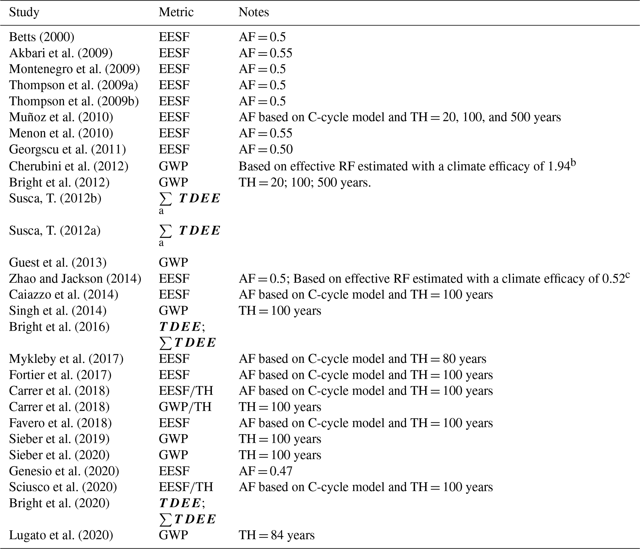
^a Referred to as “time-dependent emission”. ^b From idealized climate model simulations of Arctic snow albedo change (Bellouin and Boucher, 2010). ^c From idealized climate model simulations of global LULCC (Davin et al., 2007).

3 Overview of CO₂-equivalent metrics for RF_Δα

Over the past 20 years, a variety of metrics and their permutations have been employed to express RF_Δα as CO₂ equivalence, as evidenced from the 27 studies included in this review (Table 1).

Chiefly differentiating the methods behind the metrics shown in Table 1 – described henceforth – is how time is represented with respect to both the Δα and the reference gas (i.e., CO₂) perturbations. Among the most common approaches is to relate RF_Δα to the RF following a CO₂ emission imposed on some atmospheric CO₂ concentration background, but with a fraction of the emission instantaneously removed by Earth's ocean and terrestrial CO₂ sinks by an amount defined by 1 minus the so-called “airborne fraction” (AF) – or the growth in atmospheric CO₂ relative to anthropogenic CO₂ emissions (Forster et al., 2007).

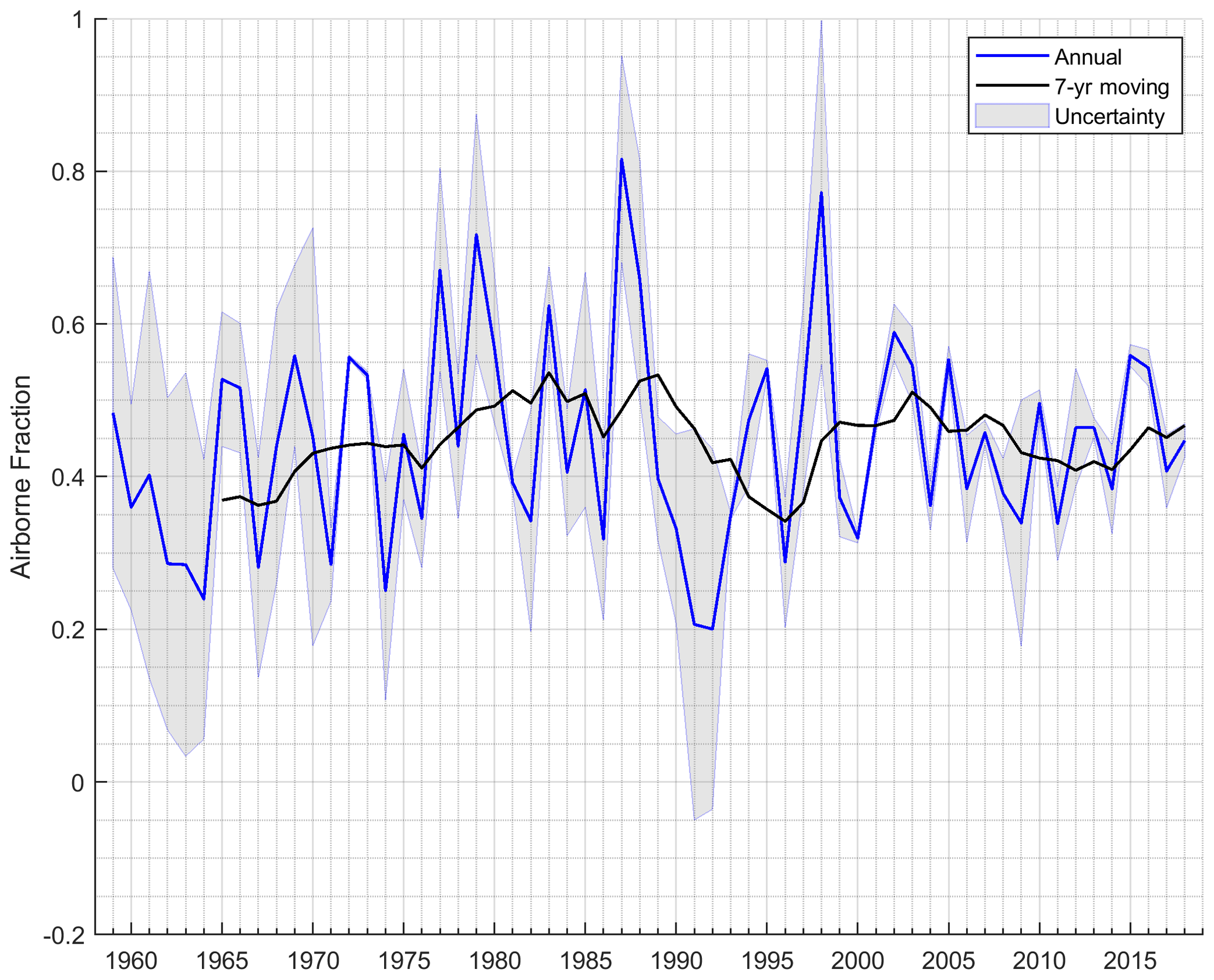
Figure 1 The 1959–2018 airborne fraction (AF), defined here as the growth in atmospheric CO₂ – or the atmospheric CO₂ remaining after removals by ocean and terrestrial sinks – relative to anthropogenic CO₂ emissions (fossil fuels and LULCC). “Uncertainty” is defined as AF ± | BI $\mathrm{|}/E$, where E is total anthropogenic CO₂ emissions and BI is the budget imbalance – or E minus the sum of atmospheric CO₂ growth and CO₂ sinks. Underlying data are from the Global Carbon Project (Friedlingstein et al., 2019).

This method – or the “emissions equivalent of shortwave forcing (EESF)” – was first introduced by Betts (2000) and may be expressed (in $\mathrm{kg}{\mathrm{CO}}_{\mathrm{2}}\text{-}\mathrm{eq}.{\mathrm{m}}^{-\mathrm{2}}$) as

$$\begin{array}{}\text{(6)}& \text{EESF}={\displaystyle \frac{{\text{RF}}_{\mathrm{\Delta }\mathit{\alpha }}}{k_{{\mathrm{CO}}_{\mathrm{2}}}{A}_{\mathrm{E}}\text{AF}}},\end{array}$$

where RF_Δα is the local annual mean instantaneous RF from a monthly Δα scenario (in W m⁻²), $k_{{\mathrm{CO}}_{\mathrm{2}}}$ is the global mean radiative efficiency of CO₂ (e.g., Eq. 2; in $\mathrm{W}{\mathrm{m}}^{-\mathrm{2}}{\mathrm{kg}}^{-\mathrm{1}}$), A_E is Earth's surface area (5.1 × 10¹⁴ m²), and AF is the airborne fraction. Because AF appears in the denominator in Eq. (6), the CO₂-equivalent estimate will be highly sensitive to the choice of AF. Figure 1 plots AF since 1959 which, as can be seen, can fluctuate considerably over short time periods, ranging from a high of 0.81 in 1987 to a low of 0.20 in 1992.

More importantly, use of AF in Eq. (6) means that time-dependent atmospheric CO₂ removal processes following emissions are not explicitly represented. However, using the AF may be justifiable in some contexts – such as when Δα has no time dependency (on inter-annual scales). For example, the pioneering study by Betts (2000) – to which almost all CO₂-eq. literature for Δα may be traced (Table 1) – made use of AF when estimating CO₂ equivalence of RF_Δα because the research objective was to compare an albedo contrast between a fully grown forest and a cropland (i.e, Δα) to the stock of CO₂ in the forest – a stock that had been assumed to accumulate over 80 years, which is the approximate time frame over which Earth's CO₂ sinks function to remove atmospheric CO₂ to a level conveniently represented by the chosen AF. Had a transient or interannual Δα scenario been modeled, however, applying the EESF method at each time step of the scenario would have severely overestimated CO₂-equivalent emissions.

For this reason, Bright et al. (2016) argued that for time-dependent Δα scenarios (i.e., when Δα evolves over interannual timescales), the time dependency of CO₂ removal processes (atmospheric decay) following emissions should be taken explicitly into account when estimating the effect characterized in terms of CO₂-equivalent emissions (or removals), thus proposing an alternate metric termed “time-dependent emissions equivalence” – or TDEE:

$$\begin{array}{}\text{(7)}& \mathit{T}\mathit{D}\mathit{E}\mathit{E}=A_{\mathrm{E}}^{-\mathrm{1}}{k}_{{\mathrm{CO}}_{\mathrm{2}}}^{-\mathrm{1}}{\mathbf{Y}}_{{\mathrm{CO}}_{\mathrm{2}}}^{-\mathrm{1}}\mathit{R}{\mathit{F}}_{\mathrm{\Delta }\mathit{\alpha }}^{\ast },\end{array}$$

where TDEE is a column vector of CO₂-equivalent emission (or removal) pulses (i.e., one-offs) with length defined by the number of time steps (e.g., years) included in the Δα time series (in $\mathrm{kg}{\mathrm{CO}}_{\mathrm{2}}\text{-}\mathrm{eq}.{\mathrm{m}}^{-\mathrm{2}}{\mathrm{yr}}^{-\mathrm{1}}$), $\mathit{R}{\mathit{F}}_{\mathrm{\Delta }\mathit{\alpha }}^{\ast }$ is a column vector of the local annual mean instantaneous RF_Δα (in W m⁻²) corresponding to the Δα time series (or RF_Δα(t)), and ${\mathbf{Y}}_{{\mathrm{CO}}_{\mathrm{2}}}$ is a lower triangular matrix with column (row) elements being the atmospheric CO₂ fraction decreasing (increasing) with time (i.e., $y_{{\mathrm{CO}}_{\mathrm{2}}}\left(t\right)$). The elements in vector TDEE thus give the CO₂-equivalent series of emission (or removal) pulses in time yielding the instantaneous RF_Δα time profile (RF_Δα(t)) corresponding to the temporally explicit Δα scenario (Δα(t)). Summing all elements in TDEE (i.e., ∑TDEE) gives a measure of the accumulated CO₂-eq. emissions (removals) over time. The TDEE approach is conceptually similar to the CO₂-forcing-equivalence (CO₂-fe) approach (Jenkins et al., 2018; Zickfeld et al., 2009) building on the notion of a “forcing equivalent” index (Wigley, 1998).

Time-dependent metrics like the well-known global warming potential (GWP) (Shine et al., 1990; Rogers and Stephens, 1988) have also been applied to characterize Δα(t), which accumulates RF_Δα(t) over time (temporally discretized) up to some policy or metric time horizon (TH), which is then normalized to the temporally accumulated radiative forcing following a unit pulse CO₂ emission over the same TH:

$$\begin{array}{}\text{(8)}& {\text{GWP}}_{\mathrm{\Delta }\mathit{\alpha }}\left(TH\right)={\displaystyle \frac{{\sum }_{\mathrm{0}}^{t=\text{TH}}{\text{RF}}_{\mathrm{\Delta }\mathit{\alpha }}\left(t\right)}{A_{\mathrm{E}}{k}_{{\mathrm{CO}}_{\mathrm{2}}}{\sum }_{\mathrm{0}}^{t=\text{TH}}{y}_{{\mathrm{CO}}_{\mathrm{2}}}\left(t\right)}},\end{array}$$

where TH is the temporal accumulation or metric time horizon. Because it is a cumulative measure, studies making use of GWP often divide by the number of time steps (TH) to approximate an annual CO₂ flux (e.g., Carrer et al., 2018). The result of Eq. (8) can be interpreted as an equivalent pulse of CO₂ (in $\mathrm{kg}{\mathrm{CO}}_{\mathrm{2}}\text{-}\mathrm{eq}.{\mathrm{m}}^{-\mathrm{2}}$) at t = 0 giving the same time-integrated RF at TH as that following a 1 kg pulse of CO₂.

3.1 Metric permutations

Some studies have applied various permutations of the three metrics presented above. For instance, some have applied definitions of the airborne fraction (AF) based on CO₂'s pulse response function (i.e., $y_{{\mathrm{CO}}_{\mathrm{2}}}\left(t\right)$) when estimating EESF on the grounds that the analysis required a long and forward-looking time perspective (Caiazzo et al., 2014; Favero et al., 2018; Mykleby et al., 2017; Muñoz et al., 2010; Sciusco et al., 2020). A consequence is that the magnitude of the CO₂-eq. calculation is highly sensitive to the subjective choice of the TH chosen as the basis for the AF (typically taken as the mean atmospheric fraction for the period up to TH – or ${\text{TH}}^{-\mathrm{1}}{\int }_{t=\mathrm{0}}^{t=\text{TH}}{y}_{{\mathrm{CO}}_{\mathrm{2}}}\left(t\right)\mathrm{d}t$). Other permutations include the normalization of EESF or GWP(TH) by TH to arrive at a uniform time series of CO₂-eq. pulses (Carrer et al., 2018) or the summing of TDEE up to TH to obtain a CO₂-eq. stock perturbation measure (Bright et al., 2020, 2016).

Figure 2 Decision tree for Δα metrics applied in the literature included in this review.

3.2 Metric decision tree

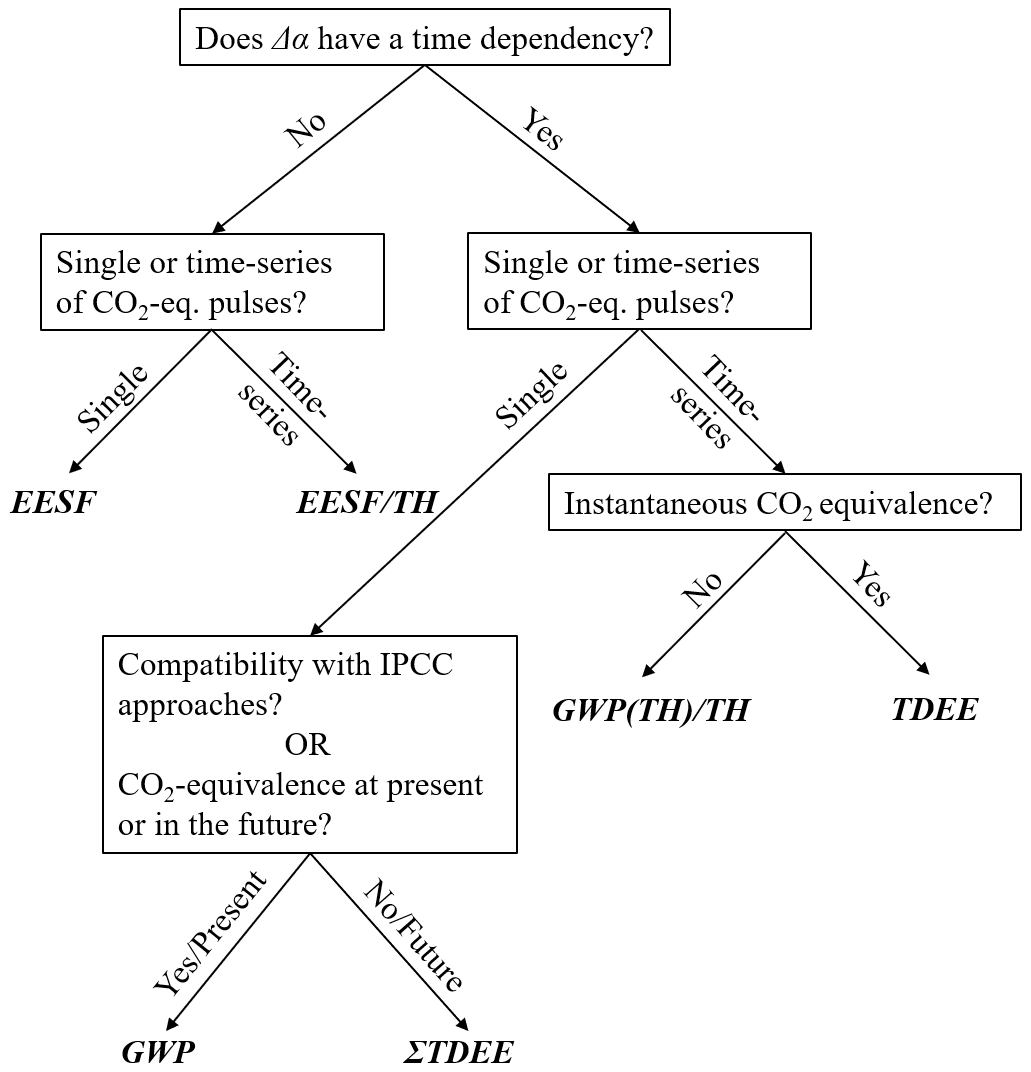
Their relative merits and drawbacks (further discussed in Sects. 4 and 5) notwithstanding, Fig. 2 presents a decision tree for differentiating between the reviewed Δα metrics presented heretofore.

A principle differentiator after the time-dependency distinction is whether CO₂ equivalence corresponds to a single emission (removal) pulse or a time series of multiple CO₂-equivalent emission (removal) pulses. For the time-dependent metrics (Fig. 2, right branch), further distinction can be made according to whether the CO₂-equivalent effect is an instantaneous effect (in the case of the time series measures) and whether IPCC compatibility is desired by the practitioner (in the case of the single pulse measures). By “IPCC compatibility”, we mean that the metric computation and physical interpretation align with emission metrics presented in previous IPCC climate assessment reports and IPCC good practice guidelines for national emission inventory reporting. A second or alternate distinction can be made for the time-dependent and single pulse measures according to whether the CO₂-equivalent effect corresponds to the present (t = 0) or the future (t = TH).

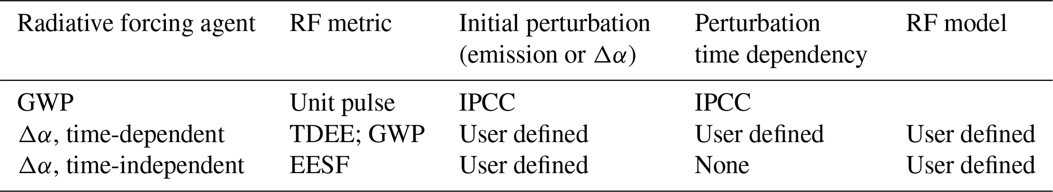
Table 2 Important decisions required by the practitioner to obtain a CO₂-eq. metric for Δα (based on RF) relative to conventional CO₂-normalized emission metrics of the IPCC (i.e., GWP).

3.3 Δα vs. emission metrics

All metric application entails subjective user decisions, such as type of metric (i.e., instantaneous vs. accumulative; scalar vs. time series) and time horizon for impact evaluation. CO₂-eq. metrics for Δα require additional decisions by the practitioner affecting both their transparency and uncertainty, which are highlighted in Table 2.

First among these is the need to quantify the initial physical perturbation (i.e., Δα), which is irrelevant for IPCC emission metrics where the initial perturbation is a unit pulse emission. For Δα metrics, uncertainty surrounding estimates of the initial (or reference) and perturbed albedo states is introduced. Second, for the time-dependent metrics (Table 2, second row) additional uncertainty is introduced by the metric practitioner when defining the time dependency of the Δα perturbation, which may be contrasted to IPCC emission metrics where the temporal evolution of the perturbation (i.e., atmospheric concentration change) is predefined (or rather, lifetimes and decay functions of the various forcing agents). Likewise, the RF models employed to give radiative efficiencies for various forcing agents are predefined by the IPCC – models having origins linked to standardized experiments employing rigorously evaluated radiative transfer and/or climate models, which may be contrasted to the models applied to estimate RF_Δα, which can vary widely in their complexity and uncertainty (for a brief review of these, see Bright and O'Halloran, 2019).

4 Quantitative metric evaluation

The metrics presented in Sect. 3 are systematically compared quantitatively henceforth by deriving them for a set of common cases, starting first with the metrics applied to yield a series of CO₂-eq. pulse emissions (or removals) in time. For all calculations, the assumed climate “efficacy” (Hansen et al., 2005) – or the global climate sensitivity of RF_Δα relative to ${\text{RF}}_{{\mathrm{CO}}_{\mathrm{2}}}$ – is 1.

Figure 3 Example application of metrics yielding a complete time series of CO₂-eq. pulse emissions or removals. (a) Time-dependent local Δα scenario (“Δα” = α_new−α_old). (b) The corresponding local annual mean instantaneous shortwave radiative forcing over time (RF_Δα(t)). (c) The derived metrics TDEE, GWP(100) $/$ 100, and EESF $/$ 100 for a range of airborne fractions (AF). (d) The reconstructed local annual mean RF_Δα(t) based on the values shown in panel (c) and Eq. (4). Note that the legend in panel (d) also applies to panel (c).

4.1 CO₂-eq. pulse time series measures

Let us first consider a geoengineering case where 1 m² of a rooftop is painted white during the first year of a 100-year simulation, which increases the annual mean surface albedo (Fig. 3a) for the full simulation period, resulting in a constant negative RF_Δα (Fig. 3b). The objective is to estimate a series of CO₂-eq. fluxes associated with the local RF_Δα(t).

Figure 3c presents the results after applying the relevant metrics to the common RF_Δα and time-dependent Δα scenario. To assess their fidelity or “accuracy”, the resulting CO₂-eq. series of annual CO₂ pulses (in this case removals) are used with Eq. (4) to re-construct the RF_Δα time profile (Fig. 3b). Unsurprisingly, annual CO₂-eq. removals estimated with the TDEE approach (Fig. 3c) reproduce RF_Δα exactly, and thus the two red curves shown in Fig. 3b and d are identical (note the difference in scale). Figure 3c illustrates the sensitivity of the EESF-based measure derived using an AF of 0.47 (mean of the last 7 years based on the most recent global carbon budget; e.g., Friedlingstein et al., 2019; Fig. 1) relative to a broad range of AF values (note that the result obtained using AF = 1 is referred to as the time-independent emissions equivalent (TIEE) presented in Bright et al., 2016). Irrespective of the AF value that is chosen, when applied in a forward-looking analysis utilizing a time-dependent Δα scenario with a time horizon of 100 years, the EESF approach underestimates the magnitude of the annual CO₂-eq. pulse occurring in the short term relative to TDEE (Fig. 3c) and hence also RF_Δα in the short term (Fig. 3b and d). This is because the CO₂ forcing represented as ${\text{TH}}^{-\mathrm{1}}{k}_{{\mathrm{CO}}_{\mathrm{2}}}\text{AF}$ with the EESF approach is weaker than the CO₂ forcing represented as $k_{{\mathrm{CO}}_{\mathrm{2}}}{\sum }_{t=\mathrm{0}}^{t=\text{TH}}{y}_{{\mathrm{CO}}_{\mathrm{2}}}\left(t\right)$ with the TDEE approach in the short term. For higher AF values, annual CO₂-eq. removals estimated using the EESF-based approach will underestimate the RF_Δα at each time step (Fig. 3d), despite the higher-magnitude CO₂-eq. estimate (relative to TDEE) seen in the longer term (Fig. 3c). This is owed to the lower atmospheric CO₂-equivalent abundance that is accumulated over the period when the series of annual CO₂-eq. fluxes are reduced to compensate for the higher AF.

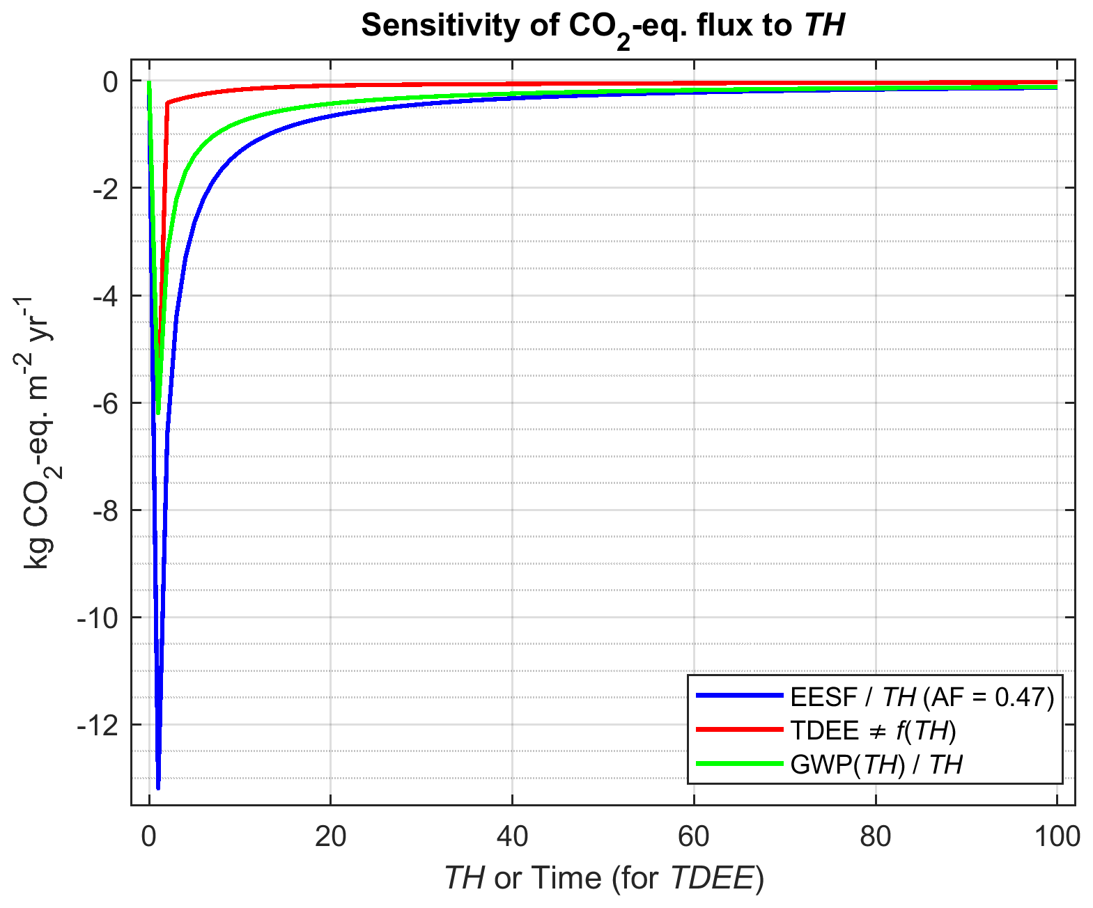
Figure 4 Magnitude of the annual CO₂-eq. emission (removal) pulse as a function of the metric TH for the EESF and GWP measures relative to TDEE, which is insensitive to TH.

For TH = 100 years, the EESF-based estimate will always be lower in magnitude in the short term and higher in magnitude in the longer term relative to TDEE (Fig. 3c). The same is also true for the annual GWP-based CO₂-eq. estimate, although at least the reconstructed RF_Δα value at t = TH will always be identical to the actual RF_Δα value at t = TH (Fig. 3d). In general, EESF- and GWP-based estimates of annualized CO₂-eq. emissions (or removals) are sensitive to the chosen TH and will always exceed (in magnitude) estimates based on TDEE. This is demonstrated in Fig. 4.

The EESF-based estimate in this example is higher (in magnitude) than the GWP-based estimate because the assumed AF of 0.47 is lower than the mean atmospheric fraction following pulse emissions (i.e., $y_{{\mathrm{CO}}_{\mathrm{2}}}\left(t\right)$) over the range of time horizons shown (the mean atmospheric fraction at TH = 100 when applying the Joos et al. (2013) function is 0.53). In contrast to the EESF- and GWP-based approaches, the magnitude of the annual CO₂-eq. removals estimated with TDEE is insensitive to the chosen TH.

4.2 Single CO₂-eq. pulse measures

Turning our attention to measures yielding a single CO₂-eq. emission or removal pulse, let us now consider a forest management case where managers are considering harvesting a deciduous broadleaved forest to plant a more productive evergreen needleleaved tree species. It is known that when the evergreen needleleaved forest matures in 80 years its mean annual surface albedo will be about 2 % lower than the deciduous broadleaved forest. The corresponding annual local RF_Δα at year 80 is 1.8 W m⁻², and we wish to associate a CO₂ equivalence with this value in order to weigh it against an estimate of the total CO₂ stock difference between the two forests after 80 years (i.e., TH = 80). Assuming we have no information about how the albedo evolves a priori in the two forests before year 80, we have no choice but to apply the EESF measure.

Figure 5 Sensitivity of EESF to the airborne fraction (AF).

Figure 5 presents the CO₂-eq. estimate based on EESF for an AF range of 0.1–1, shown together with an estimate in which the AF is obtained using the mean fraction of CO₂ remaining in the atmosphere at 80 years following an emission pulse, obtained from the latest IPCC impulse response function ($y_{{\mathrm{CO}}_{\mathrm{2}}}\left(t\right)$), and with the highest and lowest airborne fractions of the last 7 years.

Figure 5 illustrates EESF's sensitivity to the assumed AF. For instance, EESF with AF = 0.3 is double that estimated with AF = 0.6 – a normal AF range for the past 60 years (Fig. 1). EESF estimated using AF from 2015 (Fig. 5, green diamond) is 44 % lower than EESF using AF from the previous year (Fig. 5, magenta diamond). If surface albedo is ever to be included in forestry decision making – as some have proposed (Thompson et al., 2009a; Lutz and Howarth, 2014) – the subjective choice of the AF becomes problematic given this large sensitivity. For instance, if the decision-making basis in this example depends on the net of the CO₂-eq. of Δα and a difference in forest CO₂ stock of 4.5 kg CO₂ m⁻², adopting an AF of 0.5 might lead to a decision to plant the new tree species given that the stock difference would exceed the EESF estimate (i.e., CO₂ sinks dominate), whereas adopting an AF of 0.4 might lead to a decision to forego the planting given that the CO₂-eq. of Δα would exceed the stock difference (i.e., surface albedo dominates).

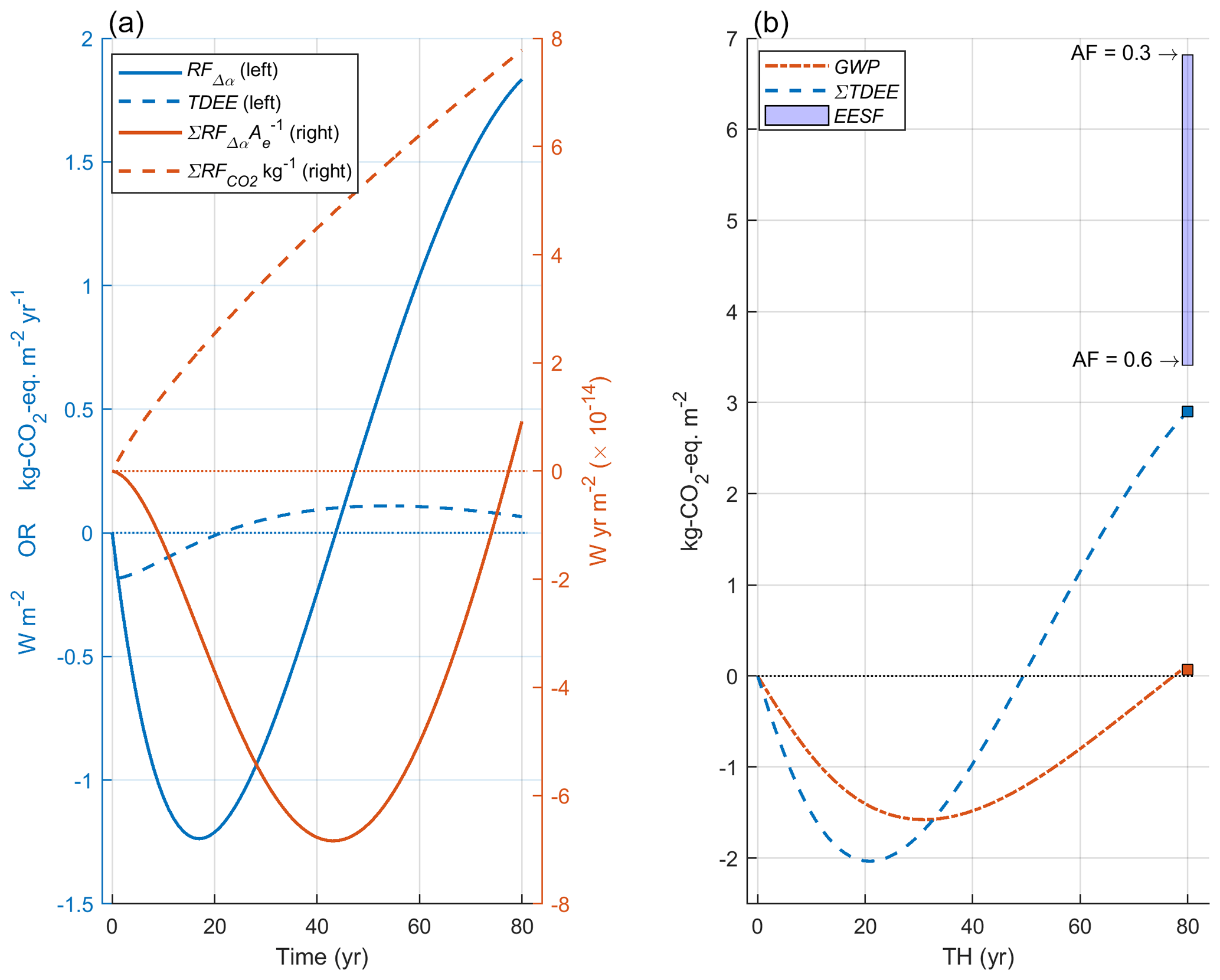
Figure 6 Example application of metrics yielding a single CO₂-eq. emission (or removal) pulse following a hypothetical forest tree species conversion. (a) RF_Δα(t) and corresponding TDEE (left y axis, blue curves) and the temporally accumulated RF_Δα(t) normalized to Earth's surface area (solid red, right y axis) and temporally accumulated ${\text{RF}}_{{\mathrm{CO}}_{\mathrm{2}}}\left(t\right)$ (dashed red, right y axis) following a 1 kg pulse emission. (b) EESF estimated for the Δα (and RF_Δα) occurring at TH = 80 shown in relation to GWP(TH) – or the ratio of two red curves shown in panel (a) – and ∑TDEE estimated at all THs.

Now let us assume the metric user does have insight into how the surface albedos of both forest types will evolve over the full rotation period. In this new example, harvesting the deciduous broadleaf forest to plant an evergreen needleleaf species will first increase the surface albedo in the short term, yet as the evergreen needleleaf forest grows and tree canopies begin to close and mask the surface, the albedo difference (Δα) reverts to negative and stays negative for the remainder of the rotation. This results in an annual mean local RF_Δα(t) profile that is first negative and then positive, which is depicted in Fig. 6a (blue solid curve, left y axis).

Converting the RF_Δα(t) time profile first to a time series of CO₂-eq. emission/removal pulses (i.e., TDEE, Fig. 6 A, dashed blue curve) and then summing to year 80 gives a measure of the total quantity of CO₂-eq. emitted (or removed) at year 80 – or ∑TDEE (Fig. 6b, blue curve). ∑TDEE thus “remembers” the negative Δα in the early phases of the rotation period (short-term), leading to a lower CO₂-eq. estimate at year 80 relative to EESF estimates computed with airborne fractions of 0.66 and lower. Similarly, the GWP-based estimate remembers the negative Δα occurring in the short term; however, GWP is a normalized measure, meaning that the time-evolving radiative effects of Δα and CO₂ are first computed independently from each other prior to the CO₂-equivalence calculation, whereas for TDEE (and hence ∑TDEE) CO₂ equivalence depends directly on the time-evolving radiative effect of Δα. Framed differently, ∑TDEE remembers prior CO₂-eq. fluxes yielding the radiatively equivalent effect of the time-dependent Δα scenario, whereas the “memories” of RF_Δα and ${\text{RF}}_{{\mathrm{CO}}_{\mathrm{2}}}$ underlying the GWP-based CO₂-equivalent estimate are first considered in isolation (Fig. 6a, red curves). Hence the GWP-based CO₂-eq. estimate in this example is much lower than the ∑TDEE-based estimate since the temporally accumulated ${\text{RF}}_{{\mathrm{CO}}_{\mathrm{2}}}$ following a unit pulse emission at t = 0 (or $\mathrm{\Sigma }{\text{RF}}_{{\mathrm{CO}}_{\mathrm{2}}}$, also known as the absolute GWP or $AGW{P}_{{\mathrm{CO}}_{\mathrm{2}}}$; Fig. 6a dashed red curve) is significantly larger than the temporally accumulated RF_Δα (or ΣRF_Δα) representing brief periods of both positive and negative RF_Δα. Comparing brief or “short-lived” RFs with CO₂ RFs using GWP has been heavily criticized for reasons we discuss further in Sect. 6.

When scalar metrics are required, Fig. 6 illustrates the large inherent risk of applying a static measure like EESF to characterize Δα in dynamic systems. Moreover, for dynamic systems in which Δα's time dependency is defined a priori, Fig. 6 illustrates the importance of clearly defining the time horizon at which the physical effects of Δα and CO₂ are to be compared: GWP gives an effect measured in terms of a present-day CO₂ emission (or removal) pulse, while ∑TDEE gives an effect measured in terms of a future CO₂ emission (or removal). In other words, internal consistency between the ecological and metric time horizons is relaxed with GWP but preserved with ∑TDEE.

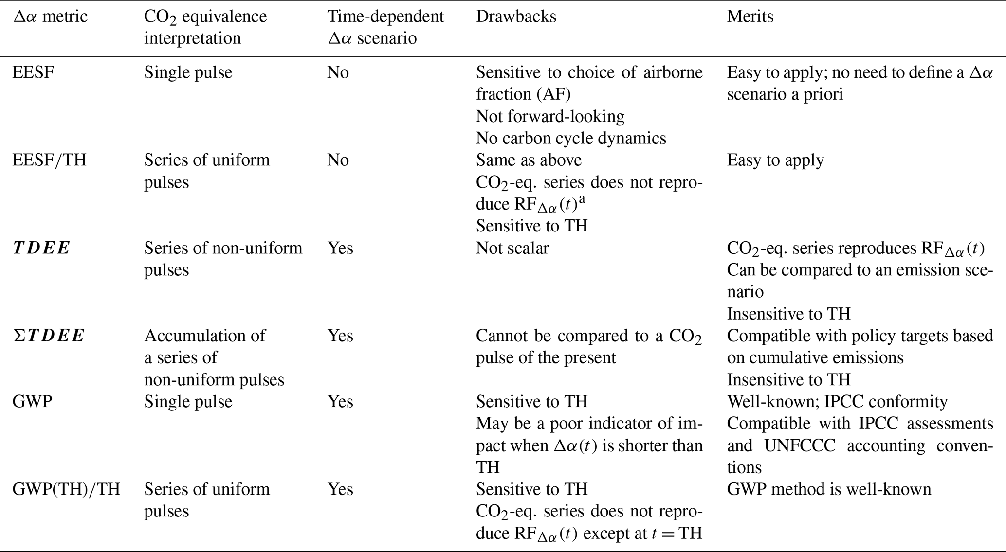
Table 3 Overview of distinguishing attributes, methodological differences, drawbacks, and merits of the six Δα metrics applied in the scientific literature included in this review.

^a The exception is at t = TH when AF = ${\text{TH}}^{-\mathrm{1}}{\int }_{t=\mathrm{0}}^{t=\text{TH}}{y}_{{\mathrm{CO}}_{\mathrm{2}}}\left(t\right)\mathrm{d}t$.

5 Qualitative metric evaluation

The reviewed metrics and underlying methods for converting shortwave radiative forcings from Δα (i.e., RF_Δα) into their CO₂-equivalent effects – summarized in Table 3 – can primarily be differentiated by the physical interpretation of the derived measure and by whether or not a time dependency (inter-annual) for Δα was defined a priori.

For cases when Δα's time dependency is not known or defined a priori, the EESF measure is the only applicable measure of those reviewed, although it was shown here to be highly sensitive to the value chosen to represent CO₂'s airborne fraction (AF; Fig. 5) – a key input variable taking on a wide range of values depending on how it was defined. In general, when AF is defined according to historical accounts of global carbon cycling, its value is prone to large fluctuations across short timescales (Fig. 1) due to natural variability in the global carbon cycle (Ciais et al., 2013). When defined as the fraction of CO₂ remaining in the atmosphere following a pulse emission – as would be obtained from a simple carbon cycle model (i.e., a CO₂ impulse response function) – its value depends on the time horizon chosen and underlying model representation of atmospheric removal processes (i.e., time constants). Use of the latter definition of AF affixes a forward-looking time dependency to the EESF measure, which is inconsistent with the definition of Δα and adds subjectivity (i.e., the choice in TH). Basing the AF on global carbon budget reconstructions would at least preserve some element of objectivity, although given the measure's sensitivity to AF it would be prudent to compute the measure for a range of AFs (i.e., as constrained by the observational record) in an effort to boost transparency. Forgoing the use of an AF altogether would eliminate all subjectivity, as has been suggested elsewhere (Bright et al., 2016).

For cases involving a time-dependent Δα scenario that is defined a priori, forward-looking measures are identified whose methodological differences give rise to different interpretations of CO₂ equivalence (Table 3). For example, the GWP measure can be interpreted as CO₂-eq. pulse emitted at present yielding the accumulated radiative forcing of the Δα scenario at TH years into the future. GWP has merit from the standpoint that it is easy to apply and conforms to established reporting methods, accounting standards, or decision-support tools such as life cycle assessment (e.g., Cherubini et al., 2012; Sieber et al., 2020). Scientifically, however, there are important limitations to GWP when the forcing (i.e., Δα) is short-lived or temporary (Allen et al., 2016; Pierrehumbert, 2014; Allen et al., 2018; Lynch et al., 2020; Cain et al., 2019). The TDEE measure, on the other hand, can be interpreted as a complete time series of CO₂ emission pulses (i.e., a complete emission scenario) yielding the instantaneous radiative forcing of the Δα scenario. When summed to TH, the latter (as ΣTDEE) provides a clearer indication of the radiative impact incurred up to TH, thus having greater scientific merit as an indicator of future warming.

The permutations of GWP and EESF applied to arrive at a time series of CO₂-eq. pulses – GWP(TH) $/$ TH and EESF $/$ TH – have little merit on the grounds that the resulting series does not reproduce RF_Δα(t) (Fig. 3d). The TDEE approach was proposed to overcome this limitation, although it should be stressed that – like GWP(TH) $/$ TH – its derivation requires that a time-dependent Δα scenario be defined a priori, which adds uncertainty and may not always be possible.

6 GWP^* and Δα

It is well known that the conventional usage of GWP does not adequately capture different behaviors of short-and long-lived climate pollutants or their impact on global mean surface temperatures (Pierrehumbert, 2014; Allen et al., 2016; Shine et al., 2003; Fuglestvedt et al., 2010). Some have proposed an alternative usage of GWP – denoted GWP^* (Allen et al., 2018) – which overcomes this problem by equating an increase in the emission rate of a short-lived climate pollutant (or radiative forcing agent) with a one-off “pulse” CO₂ emission. GWP^* recognizes that a pulse emission of CO₂ and a sudden step change in the sustained rate of emission of a short-lived climate pollutant (SLCP) both give near-constant radiative forcing. Or, alternately, that a progressive linear increase (or decrease) in the rate of an SLCP emission is approximately equivalent to a sustained step change in the emission rate of CO₂. As such, GWP^* is considered to have greater “environmental integrity” than the conventional GWP metric (Allen et al., 2018), as it is better fit to serve the purpose of a measure of progress towards a global temperature-oriented climate goal (i.e., limit warming to “well below 2 ^∘C”). Compared to conventional GWP, cumulative CO₂-eq. emissions based on GWP^* provide a clearer indication of future warming, and future CO₂-eq. emission rates better indicate future warming rates. GWP^* thus better relates all climate pollutants in a common cumulative emission (or emission budget) framework, making it easier to formulate mitigation strategies that provide a more accurate indication of progress towards climate stabilization.

Among one of the more distinguishing features of GWP^* is that, when applied to radiative forcings rather than pulse emissions, information about the time dependency of the perturbation (i.e., the lifetimes of “climate pollutants” or forcing agents) is not required (Lee et al., 2021; Cain et al., 2019; Allen et al., 2018), making it an attractive alternative to EESF. In other words, a GWP estimate of the “short-lived” forcing agent under scope – which requires such information to be known or defined a priori – is unnecessary in its calculation. Only the rate of change of the forcing is required, scaled by TH $/$ ${\text{AGWP(TH)}}_{{\mathrm{CO}}_{\mathrm{2}}}$ as follows (Lee et al., 2021; Allen et al., 2018):

$$\begin{array}{}\text{(9)}& E_{{\mathrm{CO}}_{\mathrm{2}}\text{-}\mathrm{eq}{.}^{*}}={\displaystyle \frac{\text{TH}}{{\text{AGWP(TH)}}_{{\mathrm{CO}}_{\mathrm{2}}}}}\left({\displaystyle \frac{\mathrm{\Delta }{\text{RF}}_{\mathrm{\Delta }\mathit{\alpha }}}{\mathrm{\Delta }t}}\right),\end{array}$$

where TH is the time horizon, ${\text{AGWP(TH)}}_{{\mathrm{CO}}_{\mathrm{2}}}$ is CO₂'s AGWP at the same TH (i.e., 9.2 × 10⁻¹⁴ $\mathrm{W}\mathrm{yr}{\mathrm{m}}^{-\mathrm{2}}{\mathrm{kg}}^{-\mathrm{1}}$ when TH = 100 years), Δt is the time step change, and ΔRF_Δα is the time differential of RF_Δα(t) over the step change. $E_{{\mathrm{CO}}_{\mathrm{2}}\text{-}\mathrm{eq}{.}^{*}}$ thus represents the CO₂-eq. emission pulse for the step change and will equal EESF when the AF (in Eq. 6 denominator) corresponds to the mean of $y_{{\mathrm{CO}}_{\mathrm{2}}}\left(t\right)$ over the TH (i.e., $T{H}^{-\mathrm{1}}{\int }_{t=\mathrm{0}}^{t=\text{TH}}{y}_{{\mathrm{CO}}_{\mathrm{2}}}\left(t\right)\mathrm{d}t)$. A TH of 100 years is typically applied in Eq. (9), which is justified when it exceeds the lifetime of the SLCP or when the time-integrated radiative forcing of the forcing agent (i.e, Δα) becomes a constant at this timescale, since the time-integrated radiative forcing of the reference gas (i.e., ${\text{AGWP}}_{{\mathrm{CO}}_{\mathrm{2}}}$) increases linearly with TH. In other words, the TH dependence cancels out in the calculation of ${\mathrm{CO}}_{\mathrm{2}}\text{-}\mathrm{eq}{.}^{*}$, rendering GWP^* insensitive to the choice in TH, which contrasts with the conventional GWP (Allen et al., 2016, 2018). The step change Δt for which ΔRF is calculated is typically taken as 20 years to “reduce the volatility of ${\mathrm{CO}}_{\mathrm{2}}\text{-}\mathrm{eq}{.}^{*}$ emissions in response to variations in SLCP emission rates” (Allen et al. 2018; Cain et al. 2019), although comprehensive investigations into the appropriateness of this choice when applied to a wide variety of time-varying SLCP emission (radiative forcing) scenarios are lacking. We note that more recent works (Cain et al., 2019; Lee et al., 2021) employed weighting-based modifications to Eq. (9) in an effort to better account for the longer-term temperature equilibration to past forcing changes:

$$\begin{array}{}\text{(10)}& \begin{array}{rl}{E}_{{\mathrm{CO}}_{\mathrm{2}}\text{-}\mathrm{eq}{.}^{*}}=& \left[(\mathrm{1}-s){{\displaystyle \frac{\text{TH}}{\text{AGWP(TH)}}}}_{{\mathrm{CO}}_{\mathrm{2}}}\right]{\displaystyle \frac{\mathrm{\Delta }{\text{RF}}_{\mathrm{\Delta }\mathit{\alpha }}}{\mathrm{\Delta }t}}\\ & +s{\displaystyle \frac{\stackrel{\mathrm{‾}}{{\text{RF}}_{\mathrm{\Delta }\mathit{\alpha }}}}{{\text{AGWP(TH)}}_{{\mathrm{CO}}_{\mathrm{2}}}}},\end{array}\end{array}$$

where s is a factor weighting the delayed response by global mean temperature to the radiative forcing history, represented here (following Lee et al., 2021) as the mean forcing over the period Δt – or $\stackrel{\mathrm{‾}}{{\text{RF}}_{\mathrm{\Delta }\mathit{\alpha }}}$. Note that s is analogous to the “α” term seen in Eq. (1) of Lee et al. (2021) and that the factor 1−s is analogous to the rate contribution weight denoted as “r” in Eq. (S1) of Cain et al. (2019). Like the choice of Δt, however, few investigations have been carried out to assess the appropriateness of weight sizes applied in Eq. (10) for different SLCP emission (radiative forcing) scenarios having widely varying temporal dynamics.

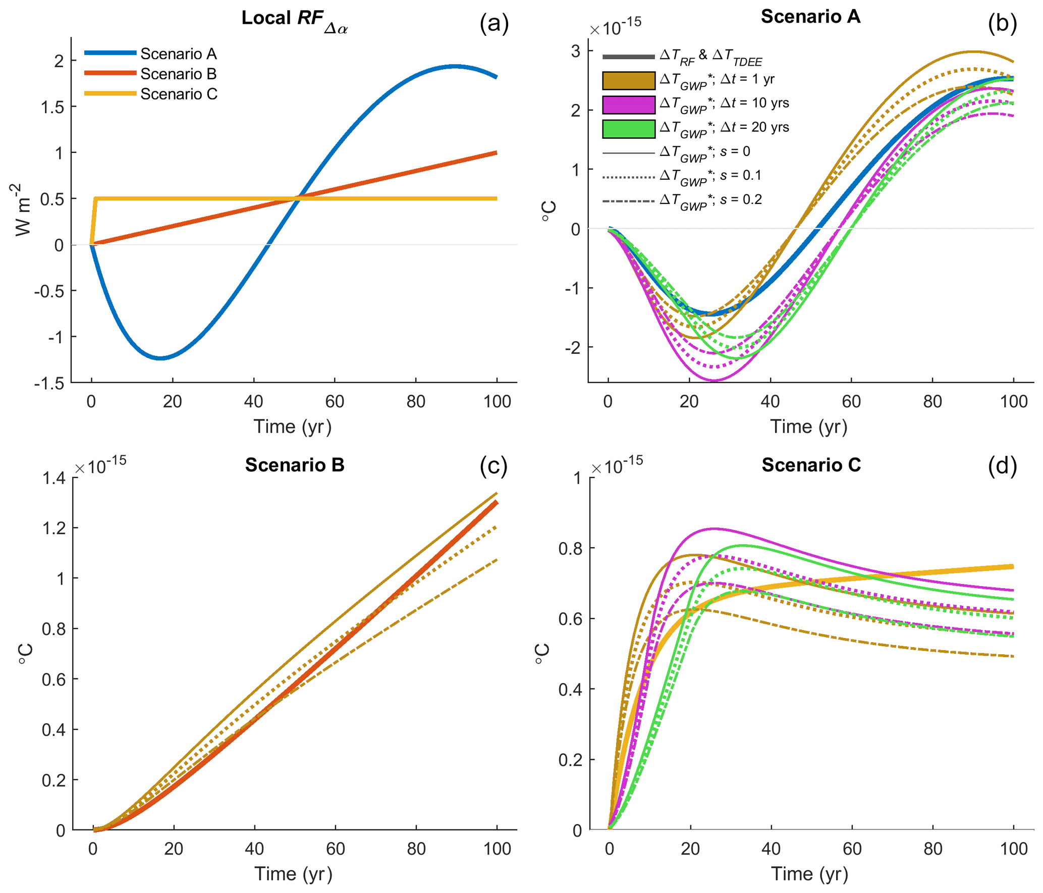
Figure 7 Performance of GWP^* computed for three stylized scenarios of surface-albedo-change-driven radiative forcing using Eq. (10) with nine different parameter sets. (a) Local radiative forcing of one permanent and two temporally evolving surface albedo change scenarios. (b–d) The corresponding global mean temperature response ΔT to the radiative forcing relative to that which has been reconstructed using the CO₂-eq. emission (removal) time series computed with TDEE and GWP^* under the assumption that $\mathrm{\Delta }{\mathit{\alpha }}_{t+n-t}$ is known. ΔT in panels (b–d) is estimated with a temperature impulse response function following Boucher and Reddy (2008) and Myhre et al. (2013) having a climate sensitivity of 1.06 $\mathrm{K}(\mathrm{W}{\mathrm{m}}^{-\mathrm{2}}{)}^{-\mathrm{1}}$, which is equivalent to a 3.9 K equilibrium climate response to an abrupt CO₂ concentration doubling.

We explore the sensitivity of the choice in both Δt and s on CO₂-eq. emissions (removals) estimated with the modified GWP^* approach (Eq. 10) for three hypothetical local RF_Δα(t) scenarios presented in Fig. 7. The first scenario – or Scenario A – is identical to the forest management scenario plotted in Fig. 6 and extended by 20 years, which is characterized by a negative RF in the short term and positive RF in the longer term (Fig. 7a, blue). In the second scenario, or Scenario B, RF_Δα(t) corresponds to a linearly increasing Δα trend which is loosely analogous to incremental deforestation occurring on a regional scale (Fig. 7a, red). The third scenario, or Scenario C, resembles a permanent albedo decrease, analogous to urban expansion into a cropland (Fig. 7a, yellow).

We then reconstruct the global mean temperature response (ΔT) of the ${\mathrm{CO}}_{\mathrm{2}}\text{-}\mathrm{eq}{.}^{*}$ emission (removal) scenario under varying assumptions surrounding the size of Δt and the weighting factor s (shown in Fig. 7b legend), which is then compared to the RF_Δα-based ΔT and the ΔT reconstructed using the CO₂-eq. emission (removal) scenario based on the TDEE approach (Fig. 7b–d). For Scenario A (Fig. 7b), we find no obvious parameter set that outperforms any other in terms of the faithfulness by which the ${\mathrm{CO}}_{\mathrm{2}}\text{-}\mathrm{eq}{.}^{*}$ emission (removal) scenario reproduces ΔT across the full time horizon. There appears to be a trade-off between the near- and long-term reproduction accuracy of different parameter sets: a 20-year Δt with no weighting (Fig. 7b, solid green curve) better reproduces the ΔT response seen in the short term (≲ 20 years) as well as the ΔT seen at the end of the scenario time horizon (year 100), whereas a 10-year Δt with no weighting (Fig. 7b, solid purple curve) better reproduces the ΔT response seen in the longer term (from ∼ 60–90 years). An increase in the weighting factor s serves to dampen the amplitude between the maximum cooling and warming seen in the short and longer term, respectively (Fig. 7b, spread between like-colored curves). As for Scenario B representing a linear increase in RF, the reconstructed ΔT is insensitive to Δt and thus only results for a 1-year Δt are computed and presented in Fig. 7c. Although a weighting factor of 0.2 is most accurate for the first ∼ 50 years, a weight of 0.1 gives a more faithful ΔT reproduction for the full time period. As for Scenario C representing a step change in RF (Fig. 7d), again we find no obvious parameter set that yields a faithful ΔT reproduction across the full time period. High s weights overpredict ΔT in the medium term but reproduce ΔT best in the longer term (Fig. 7d, solid curves), while a Δt larger than 10 years appears to result in large underpredictions in the short term (i.e., ≲ 20 years; Fig. 7d, green curves).

Unsurprisingly, ΔT reconstructed using the CO₂-eq. emission (removal) scenario estimated with the TDEE approach exactly reproduces the RF-based ΔT, and thus these two estimates are plotted jointly as a single curve in Fig. 7b–d (wider solid curves). Thus, when future surface albedo changes are defined a priori (i.e., when the Δα perturbation “lifetime” is known or estimated), a CO₂-eq. emission (removal) time series quantified with TDEE is far superior to one based on GWP^* irrespective of the choice in Δt or weight sizes applied, making it the better CO₂-eq. measure of progress towards global temperature stabilization.

Table 4 Differences in surface property and flux perturbations between geoengineering-type forcings involving non-vegetative solar radiation management (SRM) and forcings from LULCC, land management change (LMC), or forest management change (FMC). Δr_a: change to bulk aerodynamic resistance; Δr_s: change to bulk surface resistance; Δλ(E): latent heat flux change from a change to evaporation; Δλ(E+T): latent heat flux change from a change to both evaporation and transpiration; ΔH: sensible heat flux change.

7 Spatial disparity in climate response between CO₂ emissions and Δα perturbations

The climate (i.e., temperature) response to a Δα perturbation either isolated (e.g., Jacobson and Ten Hoeve, 2012) or as part of LULCC (e.g., Pongratz et al., 2010; Betts, 2001) is highly heterogeneous in space, the magnitude and extent of which depends on its location (Brovkin et al., 2013; de Noblet-Ducoudré et al., 2012). This is because the response pattern of climate feedbacks has a strong spatial dependency – feedbacks are generally larger at higher latitudes due to higher energy budget sensitivity to clouds, water vapor, and surface albedo, which generally increases the effectiveness of RF in those regions (Shindell et al., 2015). This is in contrast to CO₂ emissions where both RF and the temperature response are more homogeneous in space (Hansen and Nazarenko, 2004; Hansen et al., 2005; Myhre et al., 2013). This has caused some researchers to question the utility of a CO₂-eq. measure for Δα (Jones et al., 2013) or encouraged others to look for solutions or further methodological refinements. For instance, some researchers (e.g., Cherubini et al., 2012; Zhao and Jackson, 2014) have applied climate efficacies – or the climate sensitivity of a forcing agent relative to CO₂ (Joshi et al., 2003; Hansen et al., 2005) – to adjust RF_Δα prior to the CO₂-eq. calculation. Such adjustments recognize that the temperature response to RF depends on the geographic location, extent, and type of underlying forcing associated with the Δα (e.g., land use and land cover change (LULCC), white-roofing), which can be co-associated with other perturbations (Table 4) like those arising from changes to vegetative physical properties (for the LULCC case) which can modify the partitioning of turbulent heat fluxes above and beyond the purely radiatively driven change (Davin et al., 2007; Bright et al., 2017).

Using a climate efficacy to adjust RF_Δα, however, is not without its drawbacks. A first and obvious drawback is that efficacies are climate model dependent (Hansen et al., 2005; Smith et al., 2020; Richardson et al., 2019). Climate models vary in their underlying physics, which is evidenced by the large spread in CO₂'s climate sensitivity across CMIP6 models (Meehl et al., 2020; Zelinka et al., 2020). A second drawback is that climate sensitivities for certain forcing agents like Δα are tied to experiments that differ largely in the way forcings have been imposed in time and space. Both drawbacks contribute to large uncertainties in the choice of efficacy for Δα. The latter drawback is especially problematic since the Δα perturbation is often accompanied by perturbations to other surface properties and fluxes (Table 4) having large spatial and temporal dependencies. The turbulent heat flux perturbations that accompany a net radiative flux change at the surface affect atmospheric temperature and humidity profiles (Bala et al., 2008; Modak et al., 2016; Schmidt et al., 2012; Kravitz et al., 2013), causing the atmosphere to adjust to a new state, resulting in a net radiative flux change at TOA that extends beyond the instantaneous shortwave radiative flux change (i.e., RF_Δα).

For example, the efficacy of LULCC forcing across the six studies reviewed by Bright et al. (2015) ranged from 0.5 to 1.02 owing to differences in model set-up (e.g., fixed SST vs. slab vs. dynamic ocean), differences in the spatial extent and magnitude of the imposed LULCC forcing (e.g., historical transient vs. idealized time slice), and the LULCC definition (i.e., the type of LULCC that was included in the study such as only afforestation/deforestation vs. all LULCC). Even when controlling for differences in experimental design (e.g., CMIP protocols), the climate efficacy of historical LULCC has been found to vary considerably in both sign and magnitude (see Fig. 8, Richardson et al. 2019), which is more likely attributed to the larger spread in effective radiative forcing (ERF) for LULCC than for CO₂. For instance, Smith et al. (2020) report a standard deviation of 6 % in the ERF of CO₂ (4× abrupt) across 17 GCMs and Earth system models (ESMs) participating in RFMIP in contrast to 175 % for LULCC, although it should be kept in mind that the ERF is weak for LULCC and thus relative differences become large.

An additional drawback and source of uncertainty underlying efficacies is related to differences in their definition. Differences in definition can stem from either different definitions of RF itself or differences in the definition of the temperature response per unit RF (Richardson et al., 2019; Hansen et al., 2005). Regarding the latter, most base the temperature response for CO₂ on the equilibrium climate sensitivity (ECS) for a CO₂ doubling, although good arguments have been made for using the transient climate response (TCR) instead, particularly for short-lived forcing agents (Marvel et al., 2016; Shindell, 2014). The temperature response for the forcing agent of interest is rarely taken as the equilibrium response although there are some exceptions (e.g. “E_α” in Richardson et al., 2019, which is based on climate feedback parameters obtained from ordinary least-square regressions). Efficacies are also sensitive to the definition of RF (Richardson et al., 2019; Hansen et al., 2005). For example, the efficacy of sulfate forcing (5 × SO₄) has recently been shown to vary from 0.94 to 2.97 depending on whether RF is based on the net radiative flux change at TOA from fixed SST experiments or the instantaneous shortwave flux change at the tropopause (Richardson et al., 2019).

Ideally, CO₂-eq. metrics based on the RF concept should be based on an RF definition yielding efficacies approaching unity for a broad range of forcing types. Although there is currently no consensus here, strong arguments have been made for RF definitions based on the net radiative flux change at TOA resulting from fixed SST experiments with GCMs and ESMs (i.e., “F_s” in Hansen et al. 2005; “ERF_SST” in Richardson et al. 2019), since such definitions yield efficacies approaching unity for a broad range of forcing types. However, for most Δα metric practitioners it is not feasible to quantify atmospheric adjustments and hence the ERF. Efficacies compatible with RF_Δα (instantaneous ΔSW at TOA) could be the more feasible option for metric calculations, but broad consensus surrounding appropriate efficacy values for different forcing types associated with the Δα perturbation would need to be established first (Table 4). This is especially true for forcings involving changes to the biophysical properties of vegetation – such as LULCC, forestry, etc. – since these are constructs representing a seemingly myriad combination of perturbations acting on non-radiative controls (i.e., Δr_a and Δr_s) of the surface energy balance. Building consensus for efficacies applicable to geoengineering-type forcings where the only physical property perturbed is the surface albedo (e.g., white roofing, sea ice brightening) would be less challenging since the confounding perturbations to Δr_a and Δr_s and hence to the partitioning of the turbulent heat fluxes are removed. Nevertheless, irrespective of whether broad scientific consensus can be reached surrounding efficacies suitable for Δα metrics, additional responsibility would always be imposed on the metric practitioner to ensure that the chosen efficacy aligns with the forcing type underlying the RF_Δα.

8 Discussion

8.1 Summary of merits

In this review, we quantitatively and qualitatively reviewed metrics (methods) to characterize RF_Δα in terms of a CO₂-equivalent effect. We note that while many metrics exist, none are true “equivalents” to CO₂ due to its unique behavior. The climate effects of the calculated CO₂-eq. emissions should ideally be the same regardless of the mix of forcing agents – including Δα. However, different forcing agents have different physical properties, and a metric that establishes equivalence with regard to one effect cannot guarantee equivalence with regard to other effects and over extended time periods.

Differences among the reviewed Δα metrics could be attributed to the different ways of dealing with the time dependency of ${\text{RF}}_{{\mathrm{CO}}_{\mathrm{2}}}$, which to a large extent was determined by whether a time dependency was defined for the Δα perturbation. When the Δα perturbation was assumed to have no time dependency, as was the case for the EESF metric, uncertainties arose from the choice of AF, giving a mere snapshot in time of the CO₂ perturbation. For metrics like GWP and TDEE that explicitly account for the time dependency of ${\text{RF}}_{{\mathrm{CO}}_{\mathrm{2}}}$, the need to define a time dependency for Δα a priori introduces uncertainty owing to the reversible nature of Δα. Unlike most climate pollutants having standardized perturbation lifetimes determined by the physics of the Earth system, the perturbation lifetime of Δα is tied to a parcel of land and dictated by future anthropogenic activities occurring on that land. Users should strive to be aware of the limitations and caveats of the reviewed Δα metrics – defining a Δα time dependency might improve the precision of the CO₂-eq. estimate but not necessarily its accuracy if the future (historical) Δα cannot be confidently projected (re-constructed). Application of EESF to Δα perturbations in dynamic systems (i.e., systems in which Δα exhibits large variation over shorter timescales), on the other hand, opens up the risk for grossly mis-characterizing the system, particularly when the chosen Δα is not representative of the mean Δα of the system under scope (e.g., Fig. 6b).

Table 5 Comparison of future ΔT (global mean) from the RF_Δα(t) scenarios shown in Fig. 7a reconstructed using GWP100 and ${\sum }_{\mathrm{0}}^{\mathrm{100}}\text{TDEE}$.

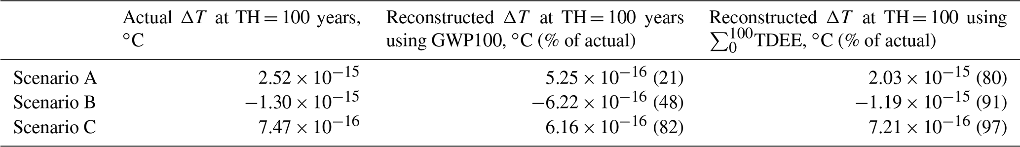
Although not applied as a Δα metric in the studies we included in our review, our review of GWP^* (Sect. 6) suggests that it is inferior to TDEE as an indicator of future warming when the future time dependency or “lifetime” of Δα is known or defined a priori (Fig. 7b). However, for cases when Δα is unknown or deemed too uncertain, one could argue that – as a scalar metric – GWP^* has greater scientific merit than EESF when applied to step changes in RF_Δα from the standpoint that CO₂'s atmospheric time dependency is taken explicitly into account. GWP – also a scalar metric – has some merit from the standpoint that it is well-known, although scientifically its merits fade when the forcing agent is short-lived (Allen et al., 2018; Lee et al., 2021; Lynch et al., 2020) – as is often the case for Δα. As a scalar metric that accounts for Δα 's time dependency, we deem ΣTDEE to have greater scientific merit than GWP because it is a better indicator of future warming, which is supported quantitatively by the ΔT reconstructions highlighted in Table 5, based on the RF_Δα(t) scenarios presented in Fig. 7a.

Although this review has provided needed guidance for choosing appropriate Δα metrics according to the context in which they have merit, users should always be mindful that ${\text{RF}}_{{\mathrm{CO}}_{\mathrm{2}}}$ and RF_Δα are not necessarily additive. The global mean temperature may respond differently to identical RFs, although there are ways to deal with this discrepancy – either by using ERFs directly in the metric calculation or by adjusting RFs with appropriate efficacy factors. Such approaches require additional modeling tools, which introduces additional uncertainties (Sect. 7). Efficacies for inhomogeneous forcings like RF_Δα are spatial-pattern- and scale-dependent (Shindell et al., 2015) and are sensitive to the climate model set-up and experimental conditions (i.e., how, where, and when Δα is imposed in the model). Moreover, efficacies are forcing-type-dependent; that is, the forcing signal driving the underlying temperature response may depend on multiple additional perturbations at the surface that are co-associated with Δα. A good example is LULCC, which perturbs a suite of additional biogeophysical properties affecting surface fluxes (Table 4), some of which result in atmospheric feedbacks (or adjustments) that can counteract the Δα -driven signal (Laguë et al., 2019). Since LULCC represents a broad range of land-based forcings, each of which in turn represent a myriad combination of surface biogeophysical property perturbations, the risk of misapplication of efficacies derived from climate modeling simulations of LULCC is inherently large.

8.2 Research roadmap

Research efforts directed towards building a scientific consensus surrounding the most appropriate RF_Δα estimation method (or model) for use in metric computation would serve to enhance metric transparency and facilitate comparability across studies. Given the ease and efficiency of applying radiative kernels for RF_Δα calculations, such efforts might entail systematic evaluations and benchmarking of radiative kernels (e.g., as in Kramer et al., 2019) for Δα.

Reducing uncertainty surrounding the efficacy of RF_Δα associated with a variety of underlying surface forcing types (i.e., specific LULCC conversions, geoengineering methods) is paramount to reducing the “additivity” uncertainty (Jones et al., 2013) of RF-based metrics for Δα. This can be achieved through extending existing climate modeling experimental protocols (e.g., LUMIP, GeoMIP, RFMIP) or by creating new protocols that seek to systematically quantify the sensitivity of the global mean temperature response to variations in the spatial pattern, extent, and magnitude of surface and TOA radiative forcings associated with Δα.

Research is also needed to examine the relevance of accounting for the climate–carbon feedback in Δα metrics, given that such feedback is implicitly included in CO₂'s impulse response function (Gasser et al., 2017). Such research should be mindful of the regional climate response patterns of the various surface forcing types associated with Δα and how regional CO₂ sinks are affected in turn by the regional response patterns.

Finally, while not a research need per se, a discussion between metric scientists and users/policy makers is needed surrounding three topics (Myhre et al., 2013): (i) useful applications, (ii) comprehensiveness, and (iii) the value of simplicity and transparency. The first involves identifying which application(s) a particular Δα metric is meant to serve. We have already shown for instance that the EESF metric is not ideal for characterizing dynamic systems. As for comprehensiveness, from a scientific point of view we would ideally wish to be informed about the totality of climate impacts of a Δα perturbation at multiple scales (i.e, at both the local and global levels). But a user may often need to aggregate this information, which necessitates trade-offs between impacts at different points in space, between impacts at different points in time, and even between the choice of metric indicator (e.g., RF vs. ΔT). Related to the value of simplicity and transparency is the question of whether more complex (yet less transparent) model-based metrics (e.g., those based on ERF) are valued by users over simple and more transparent metrics based on analytical formulations. The discussion here should weigh their trade-offs: the former may be more cumbersome to apply or more easily misused, whereas the latter may inadequately capture important physical effects or system dynamics.

8.3 Concluding remarks

For the past several decades, emission metrics have proven useful in enabling users or decision makers to quickly perform calculations of the climate impact of GHG emissions. Their common CO₂-equivalent scale has provided flexibility in emissions trading schemes and international climate policy agreements like the Kyoto Protocol. With the advent of the Paris Agreement and a broadened emphasis (Article 4) to include both emissions and removals, more attention to land-based mitigation seems likely, and the need for a way to compare albedo and CO₂ on an equivalent scale may increase. This obliges the scientific community to provide users with better tools to do so.

This review has highlighted many of challenges associated with quantifying and interpreting CO₂-equivalent metrics for Δα based on the RF concept. A variety of metric alternatives exist, each with their own set of merits and uncertainties depending on the context in which they are applied. The application of metrics always entails user choices, and while some are scientific, others – such as time frame – are policy-related and cannot be informed by science alone. This review has provided guidance to practitioners for choosing a metric with maximum scientific merit and minimum uncertainty according to the specific application context. Going forward, practitioners should always be mindful of the inherent limitations of RF-based measures for Δα, carefully weighing these against the uncertainties of metrics based on impacts further down the cause–effect chain – such as a change in temperature.