the Creative Commons Attribution 4.0 License.
the Creative Commons Attribution 4.0 License.
 | 19 May 2021
Model simulations of chemical effects of sprites in relation with observed HO2 enhancements over sprite-producing thunderstorms
Holger Winkler
Takayoshi Yamada
Yasuko Kasai
Uwe Berger
Justus Notholt
Recently, measurements by the Superconducting Submillimeter-Wave Limb Emission Sounder (SMILES) satellite instrument have been presented which indicate an increase in mesospheric HO2 above sprite-producing thunderstorms. The aim of this paper is to compare these observations to model simulations of chemical sprite effects. A plasma chemistry model in combination with a vertical transport module was used to simulate the impact of a streamer discharge in the altitude range 70–80 km, corresponding to one of the observed sprite events. Additionally, a horizontal transport and dispersion model was used to simulate advection and expansion of the sprite air masses. The model simulations predict a production of hydrogen radicals mainly due to reactions of proton hydrates formed after the electrical discharge. The net effect is a conversion of water molecules into H+OH. This leads to increasing HO2 concentrations a few hours after the electric breakdown. Due to the modelled long-lasting increase in HO2 after a sprite discharge, an accumulation of HO2 produced by several sprites appears possible. However, the number of sprites needed to explain the observed HO2 enhancements is unrealistically large. At least for the lower measurement tangent heights, the production mechanism of HO2 predicted by the model might contribute to the observed enhancements.
- Article
(3144 KB) - Full-text XML
- BibTeX
- EndNote


Sprites are large-scale electrical discharges in the mesosphere occurring above active thunderstorm clouds. Since Franz et al. (1990) reported on the detection of such an event, numerous sprite observations have been made (e.g. Neubert et al., 2008; Chern et al., 2015). Sprites are triggered by the underlying lightning, and their initiation can be explained by conventional air breakdown at mesospheric altitudes caused by lightning-driven electric fields (e.g. Pasko et al., 1995; Hu et al., 2007).
Electrical discharges can cause chemical effects. In particular, lightning is known to be a non-negligible source of nitrogen radicals in the troposphere (e.g. Schumann and Huntrieser, 2007; Banerjee et al., 2014). The chemical impact of electrical discharges at higher altitudes is less well investigated. However, it is established that the strong electric fields in sprites drive plasma chemical reactions which can affect the local atmospheric gas composition. Of particular interest from the atmospheric chemistry point of view is the release of atomic oxygen which can lead to a formation of ozone, as well as the production of NOx () and HOx (), which act as ozone antagonists.
Due to the complexity of air plasma reactions, detailed models are required to assess the chemical effects of sprites. Model simulations of the plasma chemical reactions in sprites have been presented for sprite halos (e.g. Hiraki et al., 2004; Evtushenko et al., 2013; Parra-Rojas et al., 2013; Pérez-Invernón et al., 2018), as well as sprite streamers (e.g. Enell et al., 2008; Gordillo-Vázquez, 2008; Hiraki et al., 2008; Sentman et al., 2008; Winkler and Notholt, 2014; Parra-Rojas et al., 2015; Pérez-Invernón et al., 2020). Almost all of the aforementioned studies focus on short-term effects and do not consider transport processes. One exception is the model simulation of Hiraki et al. (2008), which accounts for vertical transport and was used to simulate sprite effects on timescales up to a few hours after the electric breakdown event. There is a model study on global chemical sprite effects by Arnone et al. (2014), who used sprite NOx production estimates from Enell et al. (2008) and injected nitrogen radicals in relation with lightning activity in a global climate–chemistry model. Such an approach is suitable to investigate sprite effects on the global mean distribution of long-lived NOx. It is not useful for the investigation of the local effects of single sprites in particular regarding shorter-lived species such as HOx.
There have been attempts to find sprite-induced enhancements of nitrogen species in the middle atmosphere by correlation analysis of lightning activity with NOx anomalies (Rodger et al., 2008; Arnone et al., 2008, 2009), but until recently there were no direct measurements of the chemical impact of sprites. A new analysis of measurement data from the SMILES (Superconducting Submillimeter-Wave Limb Emission Sounder) satellite instrument indicates an increase in mesospheric HO2 due to sprites (Yamada et al., 2020). These are the first direct observations of chemical sprite effects and provide an opportunity to test our understanding of the chemical processes in sprites. The model studies of Gordillo-Vázquez (2008); Sentman et al. (2008) predict a sprite-induced increase in the OH radical in the upper mesosphere, but they do not explicitly report on HO2. The model investigation of Hiraki et al. (2008) predicts an increase in HO2 at 80 km and a decrease at altitudes 65, 70, and 75 km an hour after a sprite discharge. Yamada et al. (2020) have presented preliminary model results of an electric field pulse at 75 km which indicate an increase in HO2. In the present paper, we show results of an improved sprite chemistry and transport model covering a few hours after a sprite event corresponding to the observations of Yamada et al. (2020). The focus of our study lies on hydrogen species, and the model predictions are compared to the observed HO2 enhancements.
The SMILES instrument was operated at the Japanese experiment module of the International Space Station. It performed limb scans up to about 100 km height and took passive submillimetre measurements of various atmospheric trace gases (e.g. Kikuchi et al., 2010; Kasai et al., 2013). The size of the antenna beam at the tangent point was of the order of 3 and 6 km in the vertical and horizontal directions, respectively (Eriksson et al., 2014). The analysis of SMILES data by Yamada et al. (2020) shows an increase in mesospheric HO2 over sprite-producing thunderstorms. We provide a brief summary of the results here; further details can be sought from the original article. Three thunderstorm systems have been found for which there was a sprite observation by the Imager of Sprites and Upper Atmospheric Lightnings (ISUAL, Chern et al., 2003) on board the FORMOSAT-2 satellite followed by a SMILES measurement in spatio-temporal coincidence with the sprite detection. Table 1 shows the key parameters of the measurements. In all three cases, the total enhancement of HO2 is of the order of 1025 molecules inside the field of view of the SMILES instrument. As shown by Yamada et al. (2020), the retrieved total HO2 enhancements are basically independent on the assumed volumes in which HO2 is increased. The authors evaluated the impact of a possible contamination of the spectral HO2 features on the retrieved HO2 enhancement to be of the order of 10 %–20 %. HO2 is the only active radical for which an effect was observed. SMILES spectra of H2O2 and HNO3 have been analysed, but there are no perturbations around the events due to very weak line intensities. Note that the sprite locations lie outside the SMILES measurement volumes. The shortest horizontal distances between the SMILES lines of sight and the sprite bodies have been estimated to be about 10 km (events A and C) and 110 km (event B). There is a time lag of 1.5 to 4.4 h between the sprite detection and the SMILES measurement. Considering typical horizontal wind speeds in the upper mesosphere, Yamada et al. (2020) estimated advection distances of a few 100 km for the sprite air masses during the elapsed times between sprite occurrence and SMILES measurement. Data from the Worldwide Lightning Location Network (WWLLN) indicate strong lightning activity in the respective thunderstorm systems, and Yamada et al. (2020) pointed out that possibly additional sprites occurred which were not detected by ISUAL.
Table 1The three events analysed in Yamada et al. (2020). HW is the horizontal width of the sprites emissions, LT is the local time of the SMILES measurement, Δt is the time difference between the sprite observation and the SMILES measurement, Δr is the shortest distances between the field of view of the SMILES measurement and the sprite location, TH is the tangent height of the SMILES measurement, and ΔHO2 is the total enhancement along the line of sight of the SMILES measurement.
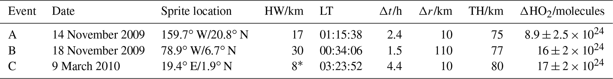
∗ Only a part of this sprite volume was observed by ISUAL (see Fig. 1 in Yamada et al., 2020).
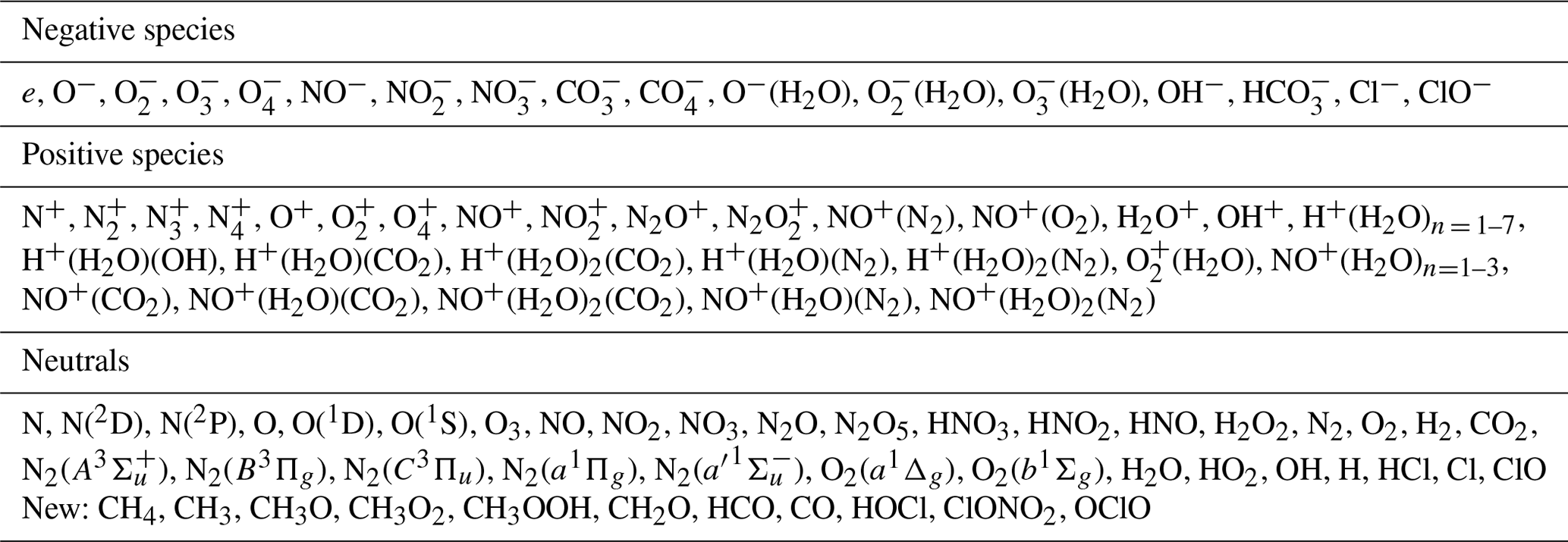
The main tool for our investigation is a one-dimensional atmospheric chemistry and transport model. It is used to simulate the undisturbed atmosphere before the occurrence of a sprite as well as the processes during and after the event. The model's altitude range is 40–120 km, and its vertical resolution is 1 km. Table 2 shows the modelled species. The model's chemistry routines are based on a model which has previously been used to simulate short-term chemical effects of sprites (Winkler and Notholt, 2014) and blue jet discharges (Winkler and Notholt, 2015). For a proper simulation of the atmospheric chemistry on longer timescales, the reaction scheme of this plasma chemistry model was merged with the one of an atmospheric chemistry model (Winkler et al., 2009) whose reaction rate coefficients were updated according to the latest JPL (Jet Propulsion Laboratory) recommendations (Burkholder et al., 2015). In the following, this model version is referred to as “Model_JPL”. For some reactions also different rate coefficients have been considered. The reason is that there are reports on discrepancies between modelled and observed concentrations of OH, HO2, and O3 in the mesosphere if JPL rate coefficients are used for all reactions (Siskind et al., 2013; Li et al., 2017). In particular, the JPL rate coefficient for the three-body reaction
where M denotes N2 or O2, appears to be too small at temperatures of the upper mesosphere. According to Siskind et al. (2013), a better agreement between model and measurement is achieved if the rate coefficient expression proposed by Wong and Davis (1974) is applied. Therefore, we have set up a model version “Model_WD” which uses the rate coefficient of Wong and Davis (1974) for Reaction (R1) while all other rate coefficients are as in Model_JPL. Li et al. (2017) have presented different sets of modified rate coefficients for Reaction (R1) as well as five other reactions of hydrogen and oxygen species. We have tested all these sets of rate coefficients in our model. In the following, we only consider the most promising model version which uses the fourth set of rate coefficients of Li et al. (2017). This model version is called “Model_Li4”. Results of the model version Model_JPL, Model_WD, and Model_Li4 will be compared in Sect. 4.
Table 2Modelled species. The last row shows the molecules additionally included compared to the model of Winkler and Notholt (2015).
The effect of the enhanced electric fields occurring in sprite discharges is accounted for by reactions of energetic electrons with air molecules. The electron impact reaction rate coefficients are calculated by means of the Boltzmann solver BOLSIG+ (Hagelaar and Pitchford, 2005); for details see Winkler and Notholt (2014). For the present study, the electron impact reactions with H2O and H2 shown in Table 4 have been added to the model.
The model has a prescribed background atmosphere of temperature, N2, and O2 altitude profiles. These profiles were derived from measurements of the SABER (Sounding of the Atmosphere using Broadband Emission Radiometry) instrument (Russell et al., 1999). The model uses daily mean daytime and night-time profiles calculated from SABER Level 2A, version 2.0, data for the geolocation of interest. At every sunrise or sunset event, the model's background atmosphere is updated.
The transport routines of the model calculate vertical transport due to molecular and eddy diffusion as well as advection. Details on the transport model can be found in the Appendix A. Transport is simulated for almost all neutral ground state species of the model. Exceptions are N2 and O2, for which the prescribed altitude profiles are used. Transport is not calculated for ions and electronically excited species as their photochemical lifetimes are generally much smaller than the transport time constants.
The abundances of neutral ground state species at the lower model boundary (40 km) are prescribed using mixing ratios of a standard atmosphere (Brasseur and Solomon, 2005). At the upper model boundary (120 km), atomic oxygen and atomic hydrogen are prescribed using SABER mixing ratios for an altitude of 105 km (the SABER O and H profiles extend only up to this altitude). This causes somewhat unrealistic conditions at the uppermost model levels; see Sect. 4. Furthermore, following Solomon et al. (1982), an influx of thermospheric NO is prescribed at the upper model boundary. For all other species a no-flux boundary condition is applied.
The one-dimensional model was used to simulate the atmosphere prior to sprite event B (Table 1). For this purpose, the model was initialised with trace gas concentrations from a standard atmosphere (Brasseur and Solomon, 2005) and then used to simulate a time period of almost 10 years before the sprite event. The background atmosphere is made of zonal mean SABER profiles of the latitude stripe 0–13.5∘ N (symmetric around the sprite latitude of 6.7∘ N) for year 2009. For this spin-up run, no ionisation is included. This allows us to use a chemical integration time step as large as 1 s. Transport is calculated once every minute.
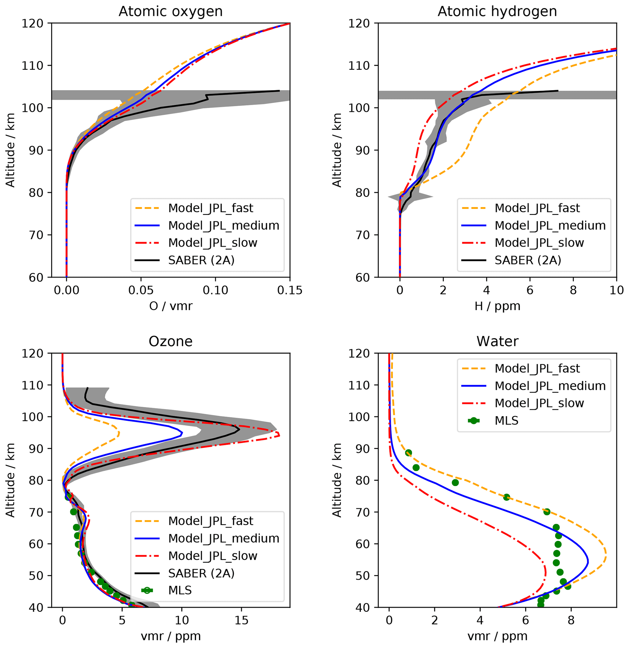
Figure 1Modelled mixing ratio profiles of selected trace gases for the undisturbed atmosphere before the sprite event B in comparison with satellite data. The model results are for 18 November 2009, 00:15 LT, solar zenith angle 165.7∘ at 6.7∘ N, 79∘ W. For all model runs, JPL rate coefficients were used. Shown are results for slow, medium, and fast vertical transport. Black solid lines show SABER Level 2A (v2) data zonally averaged night-time values for 18 November 2009 and latitudes 0–13.5∘N; the mean solar zenith angle is 160∘. The grey areas depict ±1 standard deviation of these profiles. Green data points depict MLS (Level 2, v04) zonally averaged night-time values for 18 November 2009 and latitudes 33∘ S–40∘ N; the mean solar zenith angle is 142∘.
Three model versions with different vertical transport speeds have been tested; see Appendix A for details on the transport parameters. Figure 1 shows modelled mixing ratio profiles in comparison with SABER measurements as well as measurements by the MLS (Microwave Limb Sounder) satellite instrument (Waters et al., 2006). At high altitudes, above, say, 100 km, the modelled abundances of atomic oxygen and hydrogen are too small compared to SABER profiles. This is a result of using SABER mixing ratios measured at 105 km altitude to prescribe the model's boundary values at 120 km. Test simulations have shown that the sprite altitude region is not significantly affected if different boundary conditions are used, e.g. linearly extrapolated SABER mixing ratios or O and H concentrations from the NRLMSIS-00 model (Picone et al., 2002). The model simulation with fast vertical transport agrees well with the MLS water measurements at altitudes above ∼ 75 km. On the other hand, results of this model version differ significantly from the SABER measurements of atomic hydrogen and ozone at altitudes higher than 80 km. The model simulation with medium vertical transport velocities shows a better agreement with the SABER observations. Therefore, we decided to use this model version for the sprite simulations. The agreement between the model predictions and the measurements is not perfect but reasonable for a one-dimensional model compared to zonally averaged profiles.
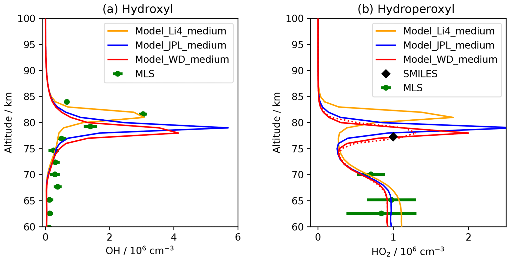
Figure 2Modelled altitude profiles of (a) OH and (b) HO2 number densities before the sprite event B in comparison with satellite data. The solid lines depict model profiles for 18 November 2009, 0:15 LT, solar zenith angle 165.7∘ at 6.7∘ N, 79∘ W. Shown are results of three model simulations with different rate coefficients for some HOx reactions (see text for details). For all model runs, medium vertical transport velocities were used. Green data points depict MLS (Level 2, v04) zonally averaged night-time values for 18 November 2009 and latitudes 33∘ S–40∘ N; the mean solar zenith angle is 142∘; the error bars correspond to 1 standard deviation. The SMILES HO2 data point corresponds to the atmospheric background value prior to the sprite event measured at 77 km (Yamada et al., 2020). Corresponding to the vertical resolution of SMILES, the dotted red line shows a 3 km running average of the red Model_WD profile.
The simulation results shown in Fig. 1 were obtained using JPL reaction rate coefficients (Model_JPL). The results of model runs with modified rate coefficients (Model_WD, Model_Li4) do not significantly differ from the results of Model_JPL in terms of the species shown in Fig. 1. However, there are considerable effects of the modified rate coefficients on OH and HO2. Figure 2 shows altitude profiles of OH and HO2 calculated with Model_JPL, Model_WD, and Model_Li4 in comparison with MLS measurements and with the SMILES HO2 atmospheric background value for sprite event B. For a comparison of absolute values, number densities are considered. There are concentration peaks of both OH and HO2 in the altitude range 75–85 km. The location and form of these peaks are affected by the changed reaction rate coefficients; see Fig. 2. The centre altitudes of the peaks are highest for the Model_Li4 simulation and lowest for the Model_WD simulation. While the Model_Li4 agrees well with MLS OH data, it significantly underestimates HO2 compared to the SMILES data point at 77 km altitude. The Model_WD agrees better with the SMILES HO2 measurement, in particular if the vertical resolution of SMILES is taken into account (Fig. 2). On the other hand, Model_WD predicts OH number densities that are too small compared to the MLS measurements.
It is not possible to draw a conclusion here on what the best set of reaction rate coefficients is. We tend to favour Model_WD as it agrees better with the SMILES HO2 data point than the other model versions. Note that the SMILES measurement corresponds to the actual geolocation and the solar zenith angle of the model profiles, whereas the MLS data points are zonal night-time averages of the latitudinal band 33∘ S–40∘ N.
We have used the model version Model_WD with medium transport velocities for the sprite simulations. The sprite has been modelled as a streamer discharge at altitudes 70–80 km. This is the core region of the considered sprite event B (see plot f in the supporting information S1 of Yamada et al., 2020). Following Gordillo-Vázquez and Luque (2010), a downward-propagating streamer is modelled by an altitude-dependent electric field time function which consists of two rectangular pulses; see Fig. 3. The first pulse represents the strong electric fields at the streamer tip, and the second pulse represents the weaker fields in the streamer channel (streamer glow region). As in the study of Gordillo-Vázquez and Luque (2010), the electric field parameters are based on results of a kinetic streamer model (Luque and Ebert, 2010).
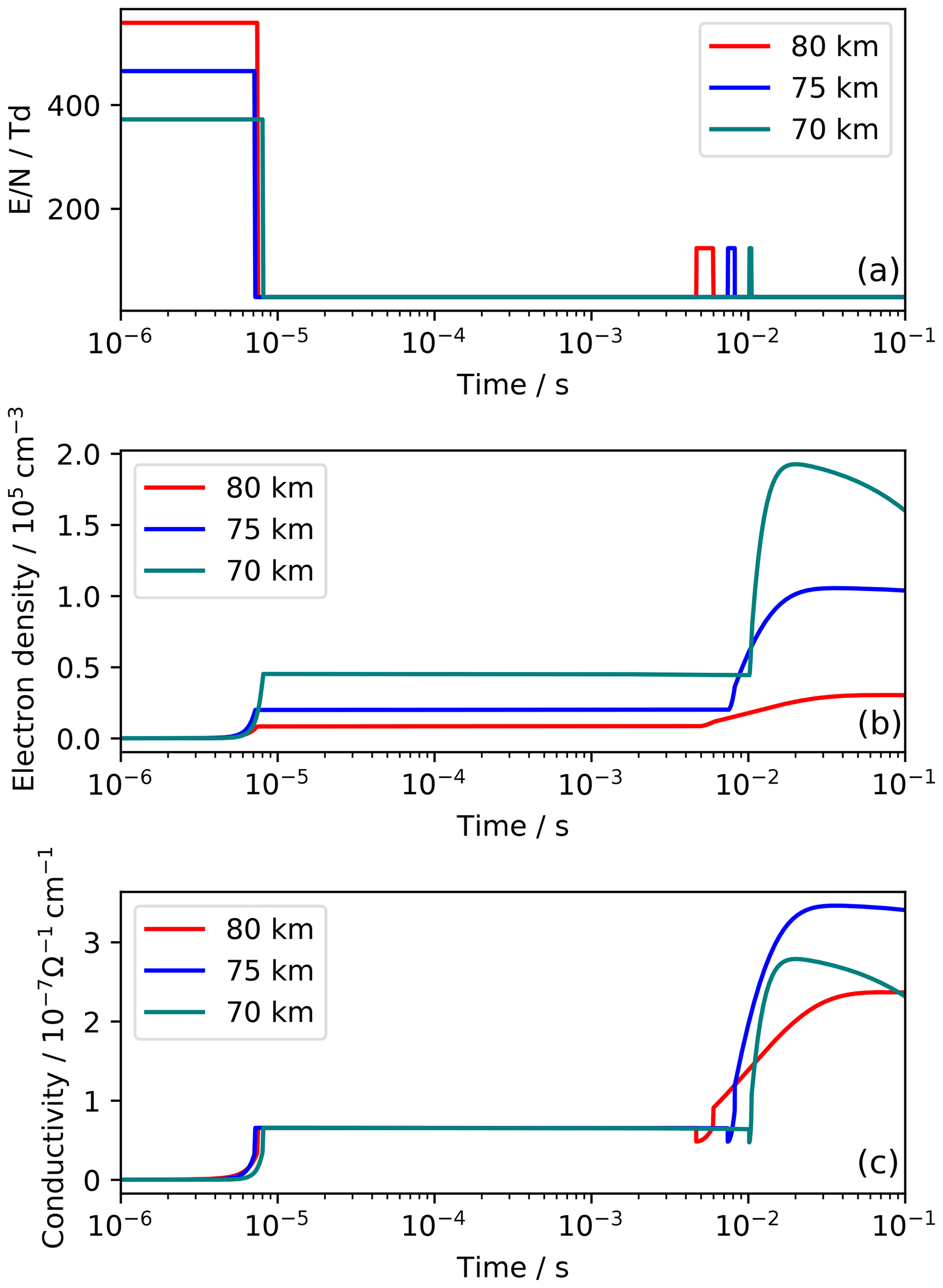
Figure 3Electric parameters of the streamer discharge as a function of time for altitudes 70, 75, and 80 km for RUN1. (a) Prescribed reduced electric field strength (in units of Td = 10−17 V cm2); (b) electron density; (c) electron conductivity.
What follows here is a description of the model's parameters in terms of the reduced electric field strength , where E is the electric field strength (V cm−1) and N is the gas number density (cm−3). The reduced electric breakdown field strength is denoted . Its value is approximately 124 V cm2. According to Luque and Ebert (2010), the reduced electric field strength at the streamer tip linearly increases with altitude. A value of is used at 70 km and at 80 km. The model is initialised with an electron density profile from Hu et al. (2007). Charge conservation is accounted for by using the same profile for the initial concentration of . The streamer tip pulse is switched off when the peak electron density in the streamer head is reached. Based on the results of Luque and Ebert (2010), the streamer head peak electron density was assumed to scale with air density, and at 75 km altitude a value of 2×10⁴ electrons per cm3 is used.
Following Gordillo-Vázquez and Luque (2010), the reduced electric field of the second pulse is taken to be at all altitudes. Between the two pulses and up to a time of 1 s after the discharge, has the sub-critical value V cm2. The altitude-dependent time lag between the pulses is determined by the different propagation velocities of streamer head and streamer tail (Gordillo-Vázquez and Luque, 2010). Three different cases of the electric fields in the streamer trailing column have been considered (Table 3). For the model “RUN1” a linearly decreasing duration of the second field pulse is assumed, ranging from 1.3 ms at 80 km to 0.3 ms at 70 km. This pulse duration is smaller than in the model of Gordillo-Vázquez and Luque (2010), who used a pulse duration of 8 ms at 80 km compared to the 1.3 ms of our RUN1. The reason for our choice of parameters is that it leads to modelled conductivities in the streamer channel which are close to the value of (Ω s)−1 reported in the literature; see Gordillo-Vázquez and Luque (2010) and references therein. Figure 3 shows the modelled electron densities and conductivities for RUN1. In order to study the effects of an increased duration time of the second pulse, a “RUN2” was performed in which the pulse is twice as long as in RUN1. This is still shorter than the pulse duration used by Gordillo-Vázquez and Luque (2010), but the resulting conductivities are already larger than in RUN1 by about a factor of 3, and it did not appear reasonable to consider even longer pulses in our model. Additionally, a model “RUN0” was performed without any second field pulse. In this simulation, there is only the breakdown electric field pulse of the streamer tip. The resulting conductivities are smaller than in RUN1 by a factor of 5 (Table 3).
Table 3Parameters of the electric field pulse in streamer trailing column at 75 km. Δt is the pulse duration, [e] the peak electron density, and σ the peak conductivity.
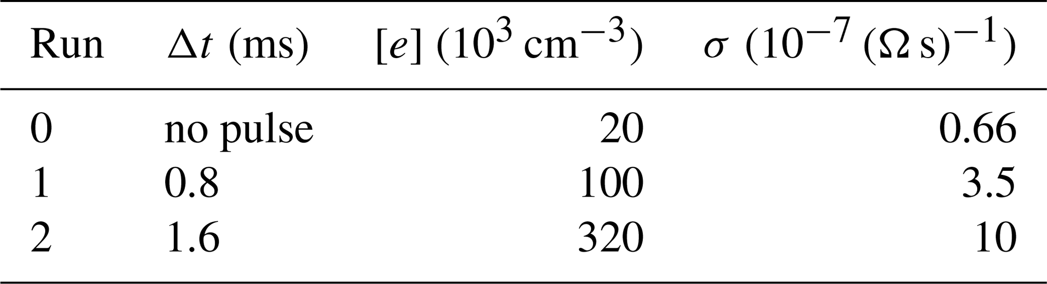
Table 4Electric-field-driven processes additionally included compared to the model of Winkler and Notholt (2014). The reaction rate coefficients in air depending on the reduced electric field strength were calculated with the Boltzmann solver BOLSIG+ (Hagelaar and Pitchford, 2005) using cross-section data for H2O (Itikawa and Mason, 2005) and for H2 (Yoon et al., 2008).
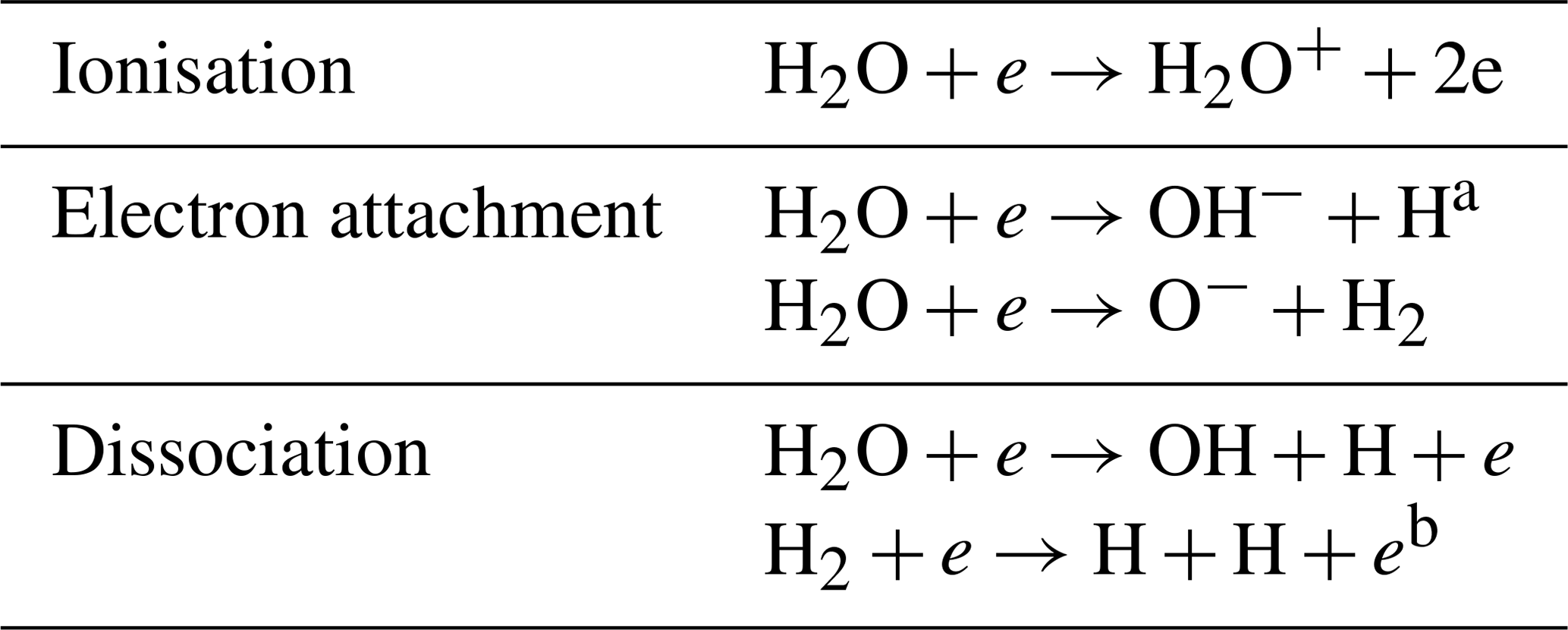
a Sum of () and (). b Sum of (), (), and ().
The model was used to simulate a time period of 5.5 h after the sprite event. It does not appear reasonable to simulate longer time periods with the one-dimensional model because eventually there is significant horizontal dispersion of the sprite air masses; see Sect. 6. For the first 2 h after the breakdown pulse, the full ion and excited species chemistry was simulated. Then, the model switched into the less-time-consuming mode without ion–chemistry (like in the spin-up run).
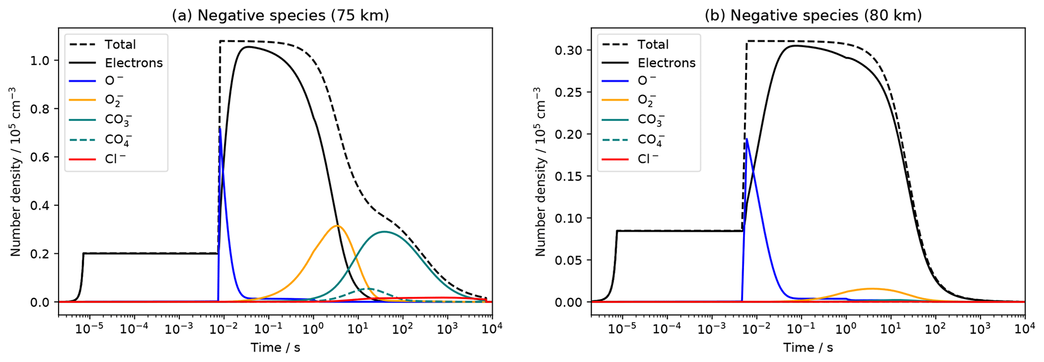
Figure 4Modelled concentrations of the most abundant negative species under the influence of the streamer electric fields for RUN1 as a function of time at (a) 75 km and (b) 80 km altitude.
First, the model RUN1 is considered. We begin our analysis of the chemical effects by an inspection of charged species. Figure 4 displays the simulated temporal evolution of the most important negative species at 80 km and at 75 km. At lower altitudes, the general pattern is similar to the one at 75 km and is therefore not shown. The streamer tip electric field pulse leads to an increase in the electron density mainly due to electron impact ionisation of N2 and O2. During the second pulse, O− becomes the main negative ion, mainly through the dissociative electron attachment process . This is followed by electron detachment reactions, of which the most efficient one is at almost all altitudes. Only at 80 km, the reaction is more important. The process
does not contribute significantly to the absolute electron detachment rates but plays a role for the hydrogen chemistry (see below). Subsequently, there is a formation of molecular ions, initiated mainly by at all altitudes. The resulting relative abundance of molecular ions is small at 80 km but larger at lower altitudes where eventually , , and Cl− become the most abundant ions. This is in overall agreement with previous model studies (e.g. Gordillo-Vázquez, 2008; Sentman et al., 2008).

Figure 5Simulated concentrations of the most abundant positive ions under the influence of the streamer electric fields for RUN1 as a function of time at (a) 75 km and (b) 80 km altitude. PHs denotes the sum of all modelled proton hydrates (). The teal solid line shows the sum of all hydrogen-containing positive ions except for proton hydrates.
Figure 5 shows the simulated temporal evolution of the most important positive ions at 80 km and at 75 km altitude. The primary ions resulting from electron impact ionisation of air molecules are and . The former undergoes rapid charge exchange (mainly) with O2 and after about one millisecond becomes the principal ion at all altitudes. This stays the same during the second electric field pulse. Eventually, there is a formation of mainly through the three-body reaction
The main loss process for are reactions with water molecules:
What follows is a formation of positive ion cluster molecules. The ion undergoes hydration reactions
which produces a proton hydrate H+(H2O)2 and releases an OH radical. Larger proton hydrates can form via successive hydration:
This is a well-known mechanism in the D region of the ionosphere (e.g. Reid, 1977) and was also predicted to take place in sprite discharges (e.g. Sentman et al., 2008; Evtushenko et al., 2013). According to our model simulations, proton hydrates have become the most abundant positive ions after a few to several seconds (depending on altitude); see Fig. 5. The speed of proton hydrate formation decreases with altitude as the three-body Reactions (R3) and (R7) are strongly pressure dependent and also because the abundance of water decreases with altitude (Fig. 1).
Recombination of proton hydrates with free electrons releases water molecules and atomic hydrogen:
The net effect of the chain of Reactions (R3)–(R8) is
As a result, there is a conversion of water molecules into two hydrogen radicals (H+OH).
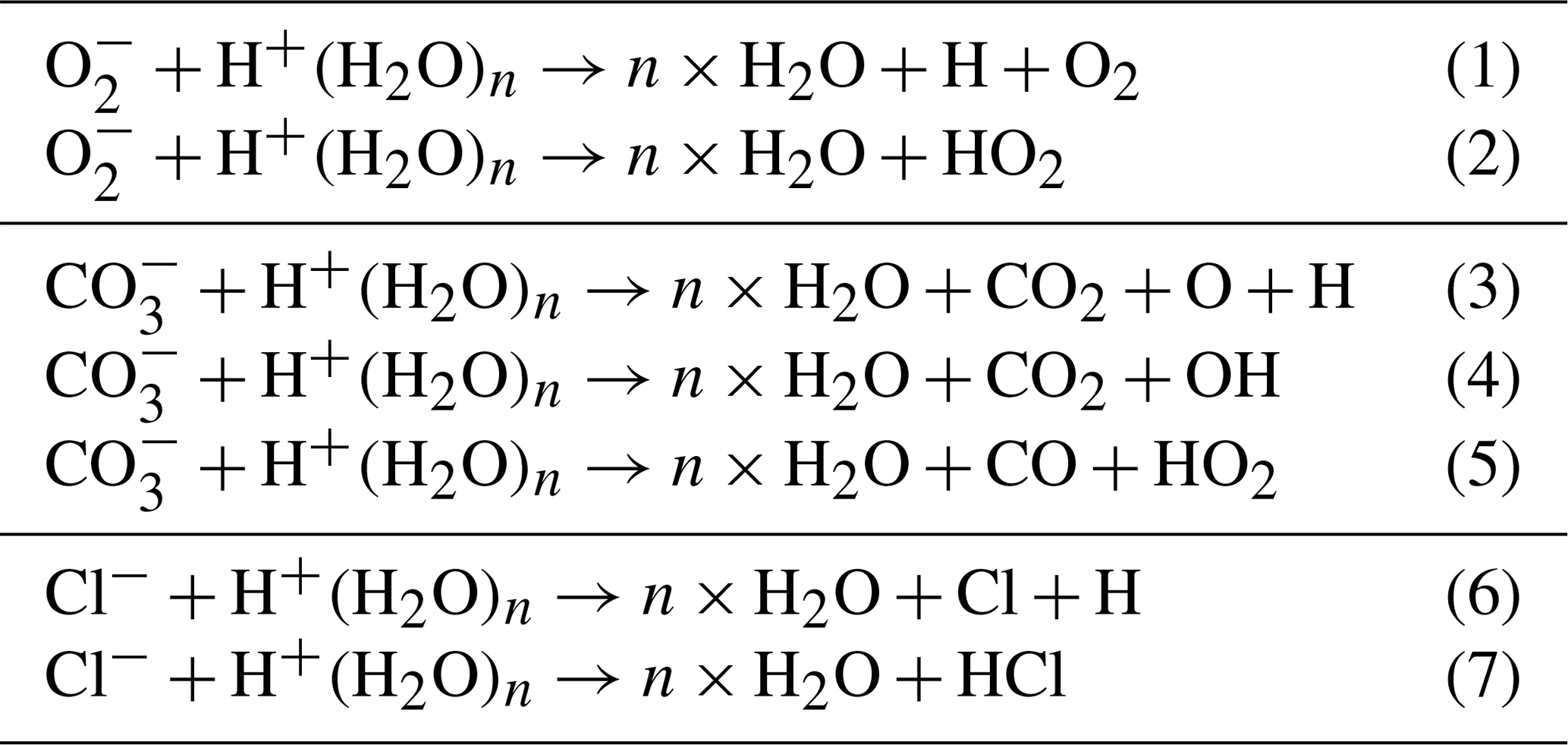
Proton hydrates can undergo recombination reactions with atomic or molecular anions as well. In the model this is accounted for by two-body and three-body recombination processes; for details see the Supplement to Winkler and Notholt (2014). In this sprite simulation, the relevant species with which proton hydrate undergo recombination are , , and Cl− (see Figs. 4 and 5). As there are uncertainties regarding some of the recombination products, we have carried out different simulations with different possible reaction products. The model results are virtually not affected by varying the recombination products according to Table 5. This shows that the branching ratios of the production of H, OH, and HO2 due to recombination is of minor importance and that the recombination with Cl− does not contribute significantly to the production of HOx (as the concentration of proton hydrates is already small when Cl− becomes the most abundant negative species).
Table 5Possible recombination reactions of proton hydrates with , , and Cl− considered in the model. Simulations have been performed for the combinations: (1)–(3)–(6), (1)–(4)–(7), (1)–(5)–(6), (1)–(5)–(7), and (2)–(5)–(6), which include cases of maximum direct HO2 formation with maximum HOx production as well as minimum direct HO2 formation with minimum HOx production.
Next we consider the impact on neutral hydrogen species. Figure 6 shows the decrease in water corresponding to the formation of hydrogen-bearing positive ions and HOx at 75 km. The effect is similar at other altitudes between 70 and 80 km. The small discontinuities of proton hydrates and HOx at a model time of 2 h are due to the end of the ion–chemical simulations (the total hydrogen amount is balanced, though). Figure 6 also displays the results of a model simulation of the undisturbed atmosphere, that is, a model run without electric fields applied. Water, hydrogen radicals, and several other species change in the no-sprite model simulation on timescales of hours (this is not a model drift but due to the fact that the night-time mesosphere is not in a perfect chemical steady state). Therefore, for a proper assessment of the sprite impact, the following analysis focuses on concentration differences between the sprite streamer simulation and the no-sprite simulation. Figure 7 shows the changes of the total amount of hydrogen atoms contained in those hydrogen species which are significantly affected by the sprite discharge at 75 km. During the first few seconds, there is a formation of positive hydrogen-bearing ions and an increase in HOx at the expense of water molecules. After about 10 s, the increase in HOx slows down, and water starts to recover.
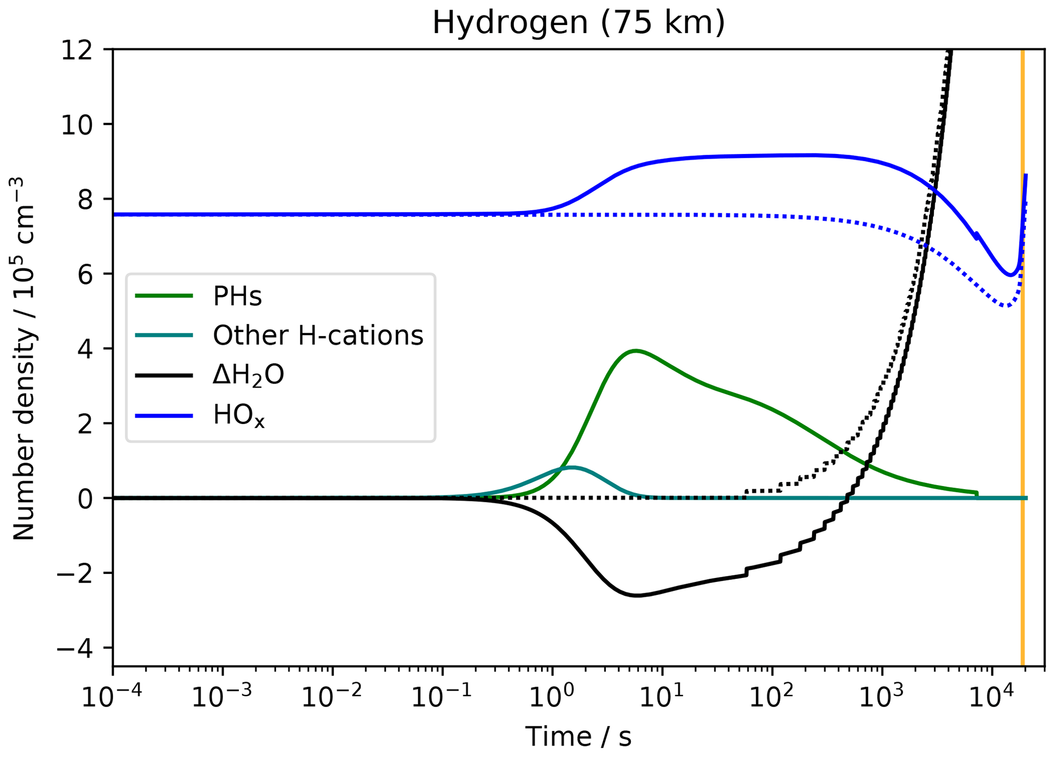
Figure 6Modelled evolution of hydrogen-containing species at 75 km altitude for RUN1. The solid lines show the sprite model run, and the dotted lines show a model run without electric fields applied. PHs denotes proton hydrates. The teal solid line depicts all hydrogen-bearing positive ions except for proton hydrates. Because of its large abundance, for water the absolute concentrations are not shown but the change of the concentration with respect to its initial value is shown. The step-like changes of H2O are due to the transport simulations once every minute. The vertical orange line indicates the time of sunrise.
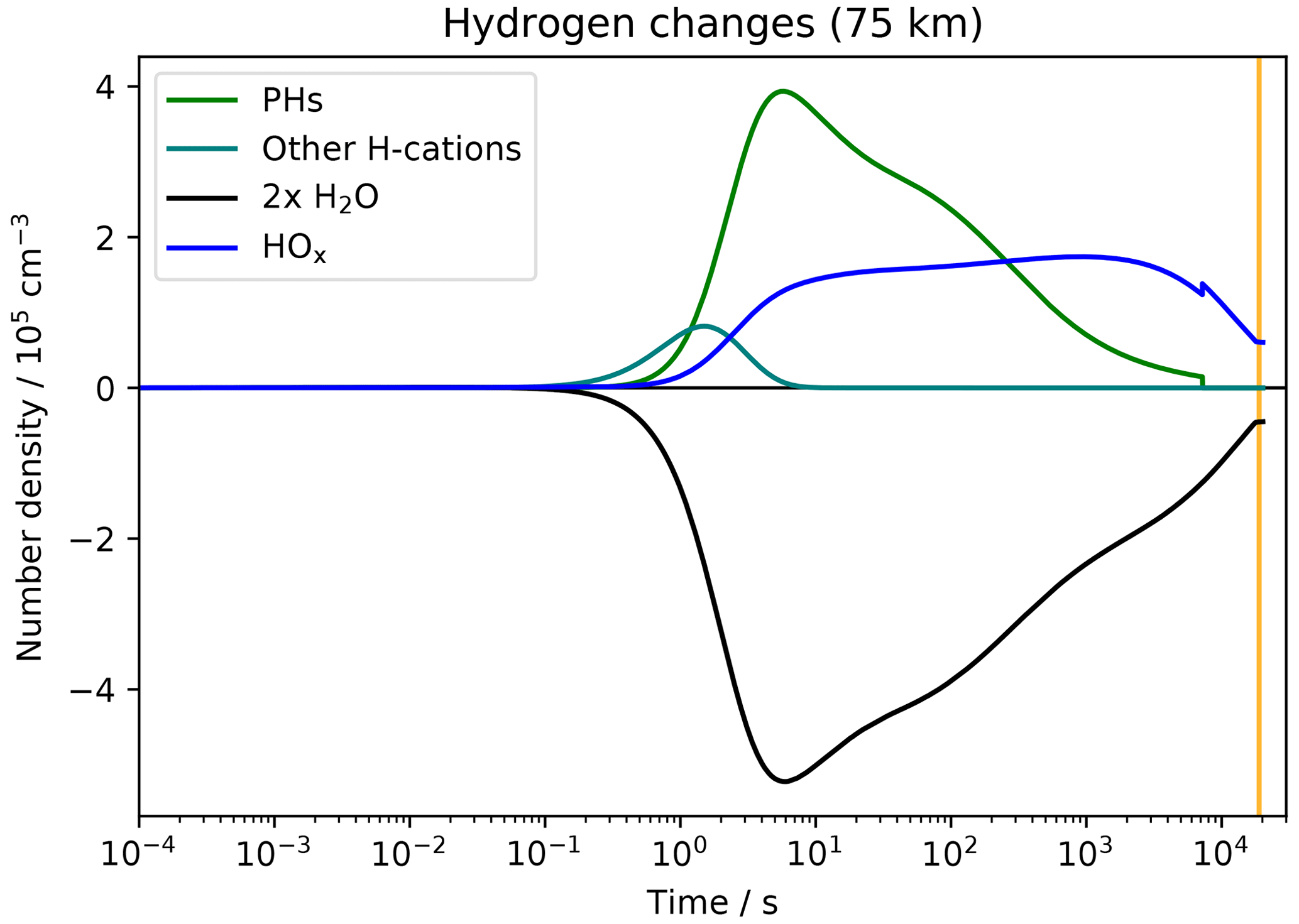
Figure 7Evolution of the modelled amount of hydrogen atoms contained in selected species at 75 km altitude for RUN1. Shown are the differences between the sprite model run and the model run without electric fields applied. PHs denotes all hydrogen atoms in proton hydrates. The teal solid line depicts all hydrogen atoms in positive ions except for proton hydrates. The vertical orange line indicates the time of sunrise.
The processes just analysed take place in the whole altitude range 70–80 km. At the highest altitudes, there is an additional process which affects the hydrogen chemistry. The already mentioned electron detachment process
causes a conversion of H2 into water molecules. This leads to a decrease in H2 at 80 km compared to the no-sprite simulation; see Fig. 8. However, the production of HOx is still mainly due to hydration reactions of positive ions. The formation of HOx molecules due to reactions of proton hydrates in the streamer at 80 km is smaller than it is at 75 km. The two main reasons for this are that (1) the total ionisation decreases with altitude (because the streamer tip peak electron density scales with air density) and (2) the formation efficiency of proton hydrates decreases with altitude (because of pressure-dependent three-body reactions and decreasing water concentrations). Both aspects can be seen in Fig. 5. Other species than the ones shown in Fig. 8 do not contribute significantly to hydrogen changes. The reactions of energetic electrons with H2 and H2O during the discharge (Table 4) are irrelevant.
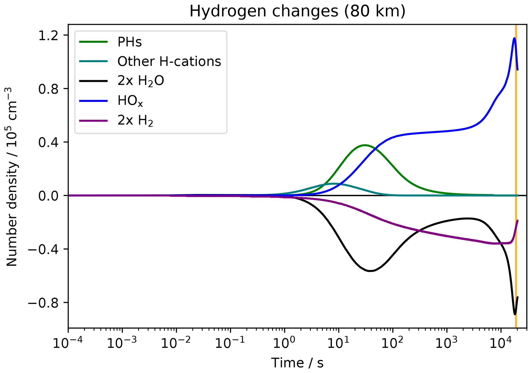
Figure 8Similar to Fig. 7 but here at 80 km and additionally showing the change of the total hydrogen amount in the form of H2 (purple line).
The temporal evolution of the different HOx species at 75 km is resolved in Fig. 9. Initially, there is an increase in both OH and H concentrations due to the ion–chemical decomposition of water molecules while the concentration of HO2 is decreased compared to the undisturbed atmosphere. The main reason for the latter is the reactions of HO2 with increased amounts of atomic oxygen produced in the sprite streamer:
On longer timescales, the concentration of HO2 slightly increases above ambient values. The most important production process at all altitudes is the three-body reaction
Figure 10 displays HO2 concentrations in the sprite streamer at altitudes 70, 75, and 80 km. The sprite effect on HO2 at 80 km is negligible.
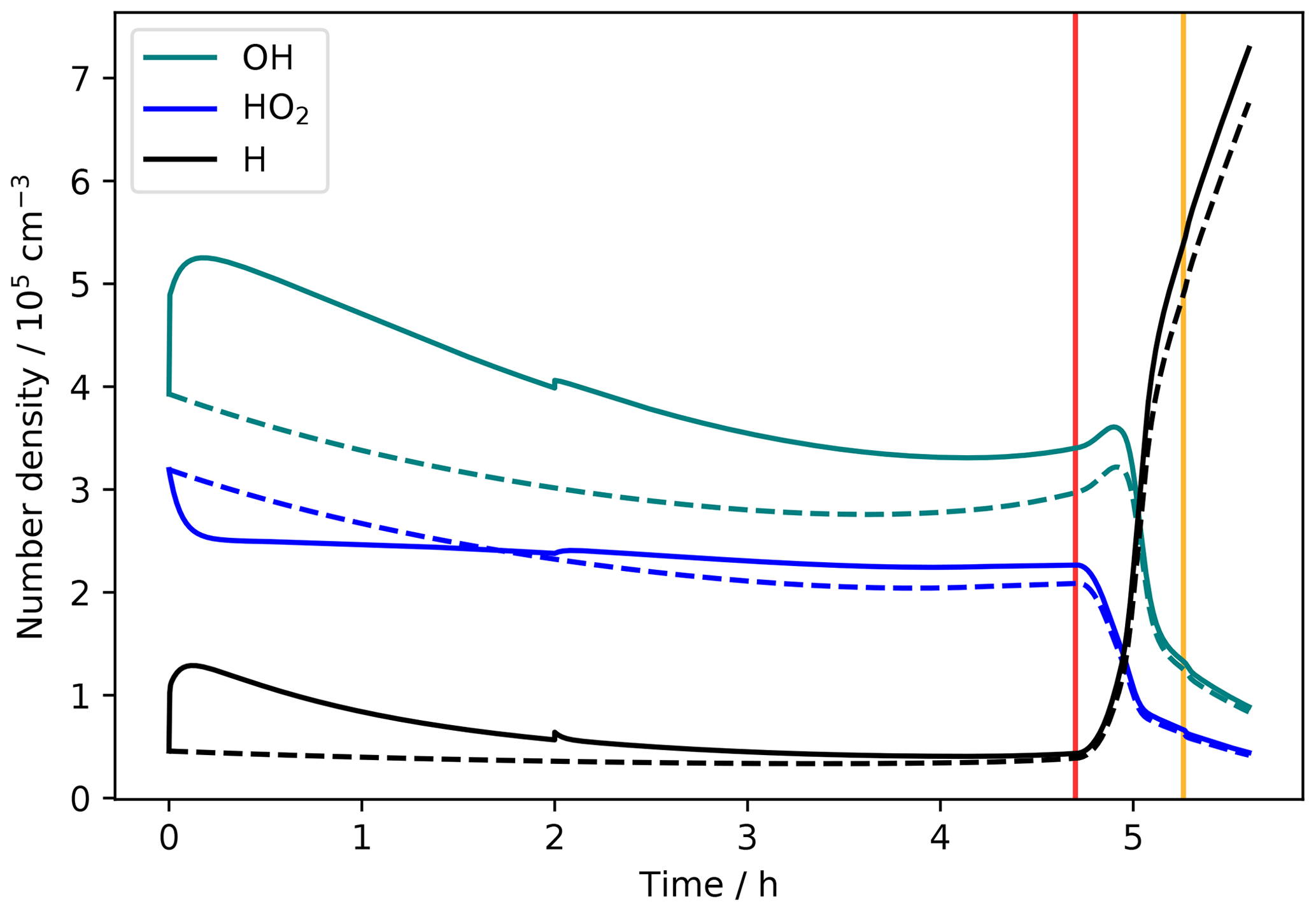
Figure 9Concentrations of H, OH, and HO2 at 75 km altitude for RUN1. The solid lines depict the sprite model simulation, and the dashed lines depict the no-sprite simulation. The vertical orange line indicates the time of sunrise, and the vertical red line indicates the time when the model starts to account for scattered sunlight (at a solar zenith angle of 98∘).
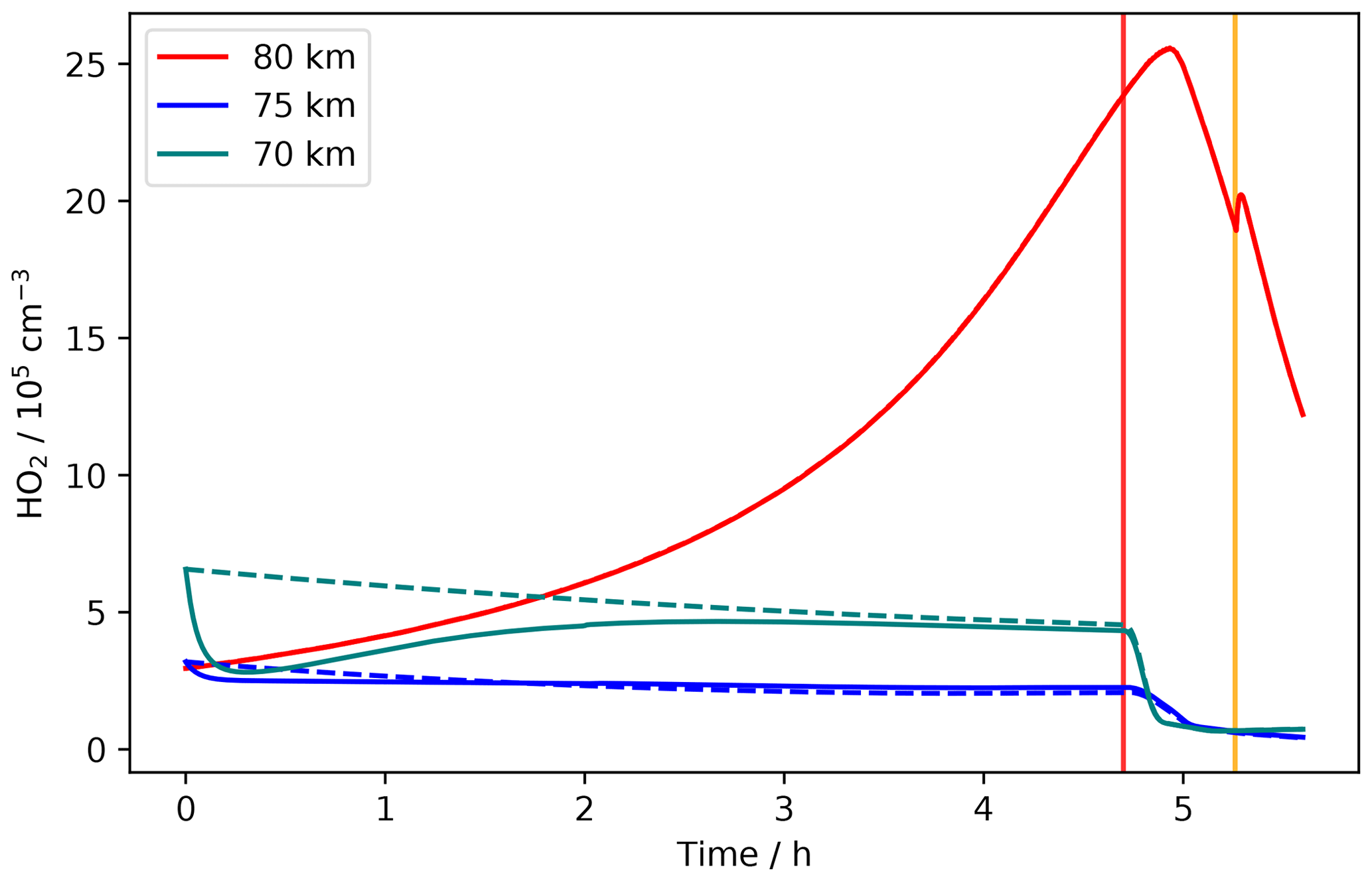
Figure 10Concentrations of HO2 at altitudes 70, 75, and 80 km for RUN1. The solid lines depict the sprite model simulation, and the dashed lines depict the no-sprite simulation (at 80 km the lines lie on top of each other). The vertical orange line indicates the time of sunrise, and the vertical red line indicates the time when the model starts to account for scattered sunlight (at a solar zenith angle of 98∘).
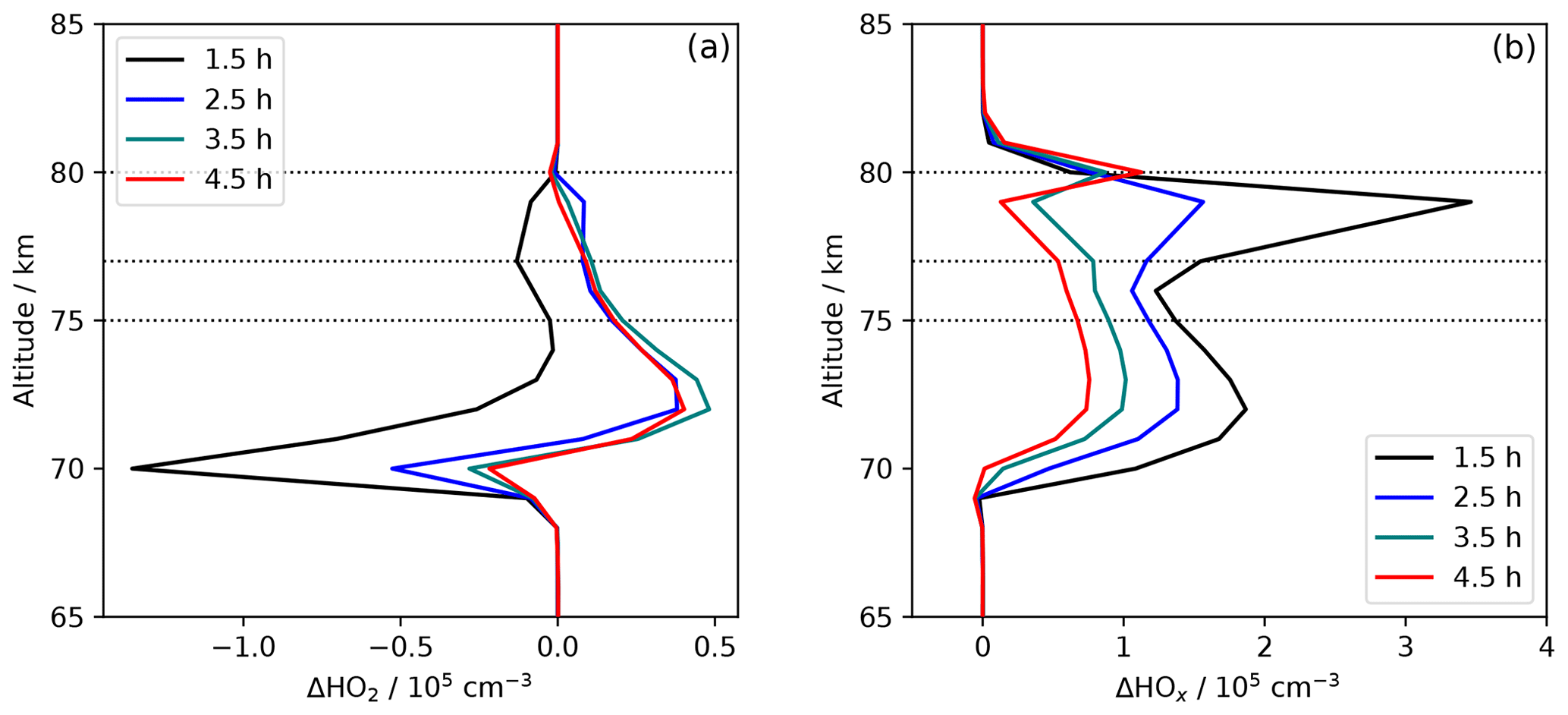
Figure 11Concentration differences between sprite and no-sprite simulation as a function of altitude for different times after the sprite discharge for RUN1. (a) ΔHO2; (b) ΔHOx. The dashed lines marks the SMILES measurement tangent height altitudes of 75, 77, and 80 km.
In Fig. 11 the concentration changes of HO2 and HOx as a function of altitude are displayed for different times after the sprite event. Note that after 1.5 h, the concentration of HO2 is smaller for the sprite model run than for the no-sprite model run basically at all altitudes between 70 and 80 km. Therefore, according to this model result, the HO2 enhancement observed by SMILES 1.5 h after sprite event B can not be attributed to that event. A possible explanation could be that other sprites previously occurred near the SMILES measurement volume. On longer timescales, there is an HO2 enhancement at all altitudes between 70 and 80 km, and an accumulation of HO2 released by different sprites appears possible. Between 2.5 and 4.5 h of model time, the HO2 enhancement is basically constant (Fig. 11). At 77 km (tangent height altitude of the SMILES measurement) the increase in HO2 is of the order of 104 molecules per cubic centimetre. The largest increase of the order 5×104 cm−3 is located at altitudes 73–74 km.
Up to this point, the results of model RUN1 were considered. The mechanism of HOx production is the same in RUN0 and RUN2. The absolute numbers, however, are different. Figure 12 compares the change of HO2 at 75 km for all three model runs. The peak HO2 increase in RUN2 is about a factor of 2 higher than that of RUN1. In RUN0 the increase is smaller than in the other runs, which highlights the importance of taking the electric fields in the streamer glow region into account.
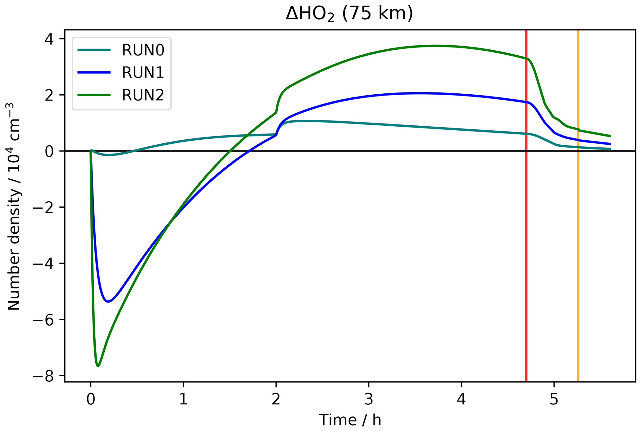
Figure 12Modelled change of HO2 at 75 km altitude for the three model simulations RUN0, RUN1, and RUN2. Shown are differences between the sprite model runs and the model simulation without electric fields applied. The vertical orange line indicates the time of sunrise, and the vertical red line indicates the time when the model starts to account for scattered sunlight (at a solar zenith angle of 98∘).
The streamer model results of this section will be used to estimate the HO2 produced by a whole sprite to compare it with the SMILES measurements in Sect. 7. Before that, the effects of advection and expansion of sprite air masses will be addressed in the next section.
As the SMILES measurements are taken a few hours after the sprite events, and at distances of several kilometres from the sprite locations, it is desirable to consider the atmospheric transport processes acting on the sprite air masses. For this purpose, we have applied a Lagrangian plume (or puff) model. This model calculates the expansion of the sprite body due to atmospheric turbulent diffusion while the sprite centre is allowed to move with the wind. Similar approaches were successfully used in research studies on air pollution plumes, aircraft trails, and rocket exhaust (e.g. Egmond and Kesseboom, 1983; Denison et al., 1994; Karol et al., 1997; Kelley et al., 2009). Our model accounts only for horizontal transport because vertical transport is already included in the one-dimensional model run presented in Sect. 5 and more importantly because the timescales of vertical transport in the mesosphere are larger than the horizontal ones by orders of magnitude (e.g. Ebel, 1980).
The advection of the sprite centre is calculated using wind field data originating from the Leibniz Institute middle atmosphere model (LIMA). LIMA is a global three-dimensional general circulation model of the middle atmosphere (Berger, 2008). It extends from the Earth's surface to the lower thermosphere. In the troposphere and lower stratosphere the model is nudged to observed meteorological data (ECMWF/ERA-40). LIMA uses a nearly triangular mesh in horizontal direction with a resolution of about 110 km. At each time step, the LIMA wind fields are linearly interpolated to the current position of the sprite centre.
The expansion of the sprite cross section is calculated by a Gaussian plume model approach (e.g. Karol et al., 1997). The radius of the plume corresponds to the standard deviation of a Gaussian concentration distribution. If wind shear effects are neglected, the temporal change of the variance σ2 is given by (Konopka, 1995)
with K being the apparent horizontal diffusion coefficient. The formation time of a sprite is short compared to the timescales of atmospheric eddy diffusion. For such an instantaneous source, the diffusion coefficient is given by (Denison et al., 1994)
where K∞ is the atmospheric macroscale eddy diffusion coefficient, t is the age of the plume, and tL is the Lagrangian turbulence timescale. The latter is connected with K∞ and the specific turbulent energy dissipation rate ε through
Based on ranges of literature values of the turbulent parameters for the upper mesosphere (Ebel, 1980; Becker and Schmitz, 2002; Das et al., 2009; Selvaraj et al., 2014) we have considered two cases:
-
a slow diffusion scenario with K∞=106 cm2 s−1 and ε=0.01 W kg−1;
-
a fast diffusion scenario with cm2 s−1 and ε=0.1 W kg−1.
The initial plume diameters were taken to be the horizontal widths of the sprites derived from the sprite observations (Table 1). Figure 13 shows results of the plume model simulations for both fast and slow diffusive sprite expansion. Only in case of sprite event C, the SMILES field of view lies inside the expanded sprite body. For the other cases there is only little or no overlap of the SMILES measurement volume and the increased sprite volume. Therefore, it is unlikely that the measured HO2 enhancements are solely due to the three observed sprites. As pointed out by Yamada et al. (2020), additional sprites may have occurred in the same region, which would allow an accumulation of HO2 released by different events.
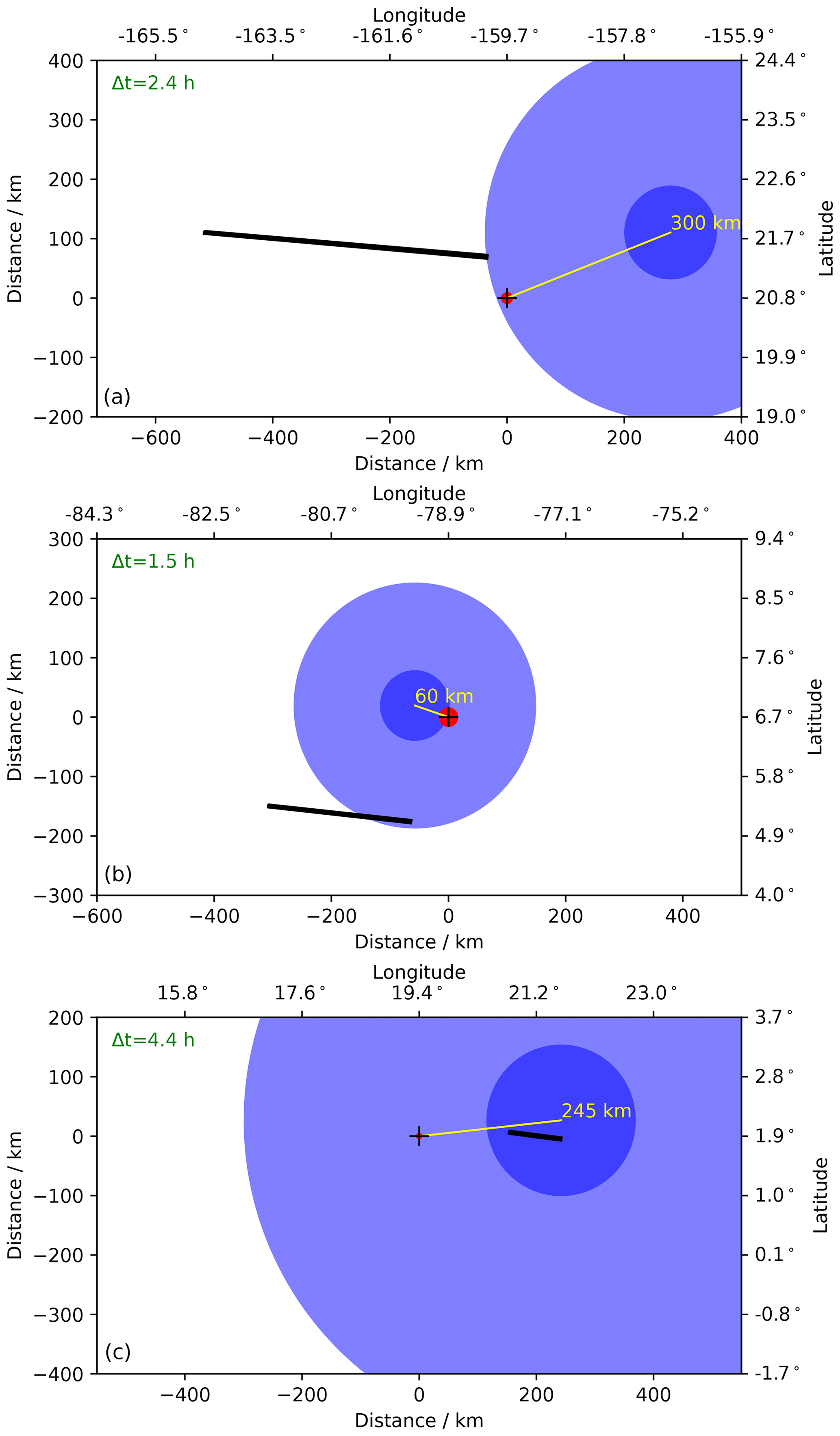
Figure 13Results of the sprite transport and dispersion calculations. From top to bottom: sprite event A, B, and C (Table 1). The axes give latitude and longitude of the scenes as well as the meridional and zonal distances from the initial sprite locations (all three maps display the same area size). The red circles depict the initial sprite cross sections derived from the observed horizontal widths of the sprites. The blue circles indicate the sprite cross sections at the times of the SMILES measurements. The large/small blue circles correspond to the fast/slow diffusion scenario. The black lines show the fields of view of the SMILES measurements (between the tangent points and an altitude of 81.5 km). The yellow lines show the displacement of the sprite centres, and Δt is the time difference between the sprite occurrence and the SMILES measurement.
The model results of Sect. 5 referred to the concentration changes inside a single sprite streamer. Now we make an attempt to estimate the resulting total ΔHO2 of the sprite event. Unfortunately, the sprite images do not allow us to infer the number of streamers or a volume filling fraction of the sprite body with streamers. We estimate these parameters by considering the emissions in the first positive band of molecular nitrogen:
A time integration of the model rates of this process yields the total number of photons emitted by a streamer in the altitude range 70–80 km (using the streamer diameter scaling of Luque and Ebert, 2010). The obtained values are ∼ 5 × 10²⁰ ∼ 1022 and ∼ 1024 photons for RUN0, RUN1, and RUN2, respectively. The large differences between these values are due to the fact that in the streamer glow region N2(B3Πg) is effectively produced by electron collisions with ground state N2.
Typically, the total number of photons in the first positive band of N2 emitted by a sprite lies in the range 1023 to a few 1024 photons (e.g. Heavner et al., 2000; Kuo et al., 2008; Takahashi et al., 2010). Assuming a value of 1024 photons emitted by the sprite event under consideration and neglecting absorption of photons inside the sprite volume yields 10 streamers for RUN1. This corresponds to a volume filling fraction of the sprite body with streamers of nearly 10 % under the assumption that the sprite was of cylindrical shape with a diameter of 30 km (Table 1). This appears to be a realistic value. For comparison, Arnone et al. (2014) assumed a higher number of 4500 streamers inside a larger sprite volume, which corresponds to a smaller volume filling fraction of 1 %. For RUN0 one yields ∼2000 streamers, which would correspond to an unrealistic volume filling fraction of ∼ 200 %. The reason for this is the missing production of N2(B3Πg) in the streamer trailing column in RUN0. For RUN2 one would yield only one streamer. This is unrealistic as well. The reason is that there is too much production of N2(B3Πg) in alignment with the electron densities and conductivities of RUN2 that are too high. Therefore, the results of RUN1 are used for the following estimations.
Integrating ΔHO2 over the sprite body yields a negative value of about −1020 molecules per 1.5 h after the event. For later times (2.5–4.5 h), a total increase of the order of 1020 molecules is obtained.
In order to compare the modelled HO2 enhancements with the SMILES observations, we estimate the total ΔHO2 inside the SMILES measurement volume. For this purpose, it is assumed that the SMILES measurement volume lies inside of an expanded sprite body. The dispersion simulations in Sect. 6 have shown that, already a few hours after the sprite events, the diameter of the expanding sprite air masses is of the same order as the length of the SMILES line of sight in the sprite altitude region. Therefore, in particular if several sprites occurred in the same region, significant overlap of the SMILES measurement volumes and expanded sprites can be expected.
For the sprite event B, the tangent height of the SMILES measurement is 77 km. The HO2 enhancement in a streamer at that altitude is ∼ 104 cm−3 for model times larger than 2.5 h (Sect. 5, Fig. 11). With a volume filling fraction of 10 %, the mean enhancement in the initial sprite volume is ∼ 103 cm−3. According to the dispersion simulations, within a few hours the volumes of the sprite air masses increase by a factor between about 10 and 1000. Therefore, the diluted ΔHO2 is in the range 1–100 cm−3. At the tangent point, the antenna beam of SMILES has an elliptical cross section of 3 km in vertical direction and 6 km in horizontal direction. With a length of ∼ 250 km of the SMILES field of view for event B (Fig. 13), the total number of excess molecules in that volume is of the order of 5 × 10¹⁹ to 5 × 10²¹. Even the largest value of that range is small compared to the observed ∼ 1.6 × 1025 molecules. A number of ∼ 3200 sprites would be required to cause such an enhancement provided that the ΔHO2 values of the single sprites add up.
For the sprite event A, the measurement tangent height is lower (75 km) than for event B, and the length of the SMILES field of view is larger (∼ 500 km, Fig. 13). At the same time, the streamer ΔHO2 is larger at that altitude. This leads to an estimated total number of HO2 excess molecules in the SMILES line of sight of 5 × 10²⁰ to 5 × 10²². The largest value is about 200 times smaller than the observed ∼ 9 × 1024 molecules.
For sprite event C, the model does not predict any noticeably increase in HO2 at the measurement tangent height of 80 km, in contrast to the SMILES measurements.
For a quantitative comparison between model and measurements, it would be necessary to know the number of sprites which occurred and affected the air masses observed by SMILES. We make an estimate of that number of sprites although the available data on the thunderstorms are very limited. Lightning properties such as polarity and electric charge moment change were not stored in the WWLLN database. Therefore, only the total number of lightning strokes is known. During the time of 4.5 to 1.5 h before the SMILES measurements, the WWLLN detected 2822, 4427, and 1507 lighting flashes in the areas of event A, B, and C shown in Fig. 13. Assuming a WWLLN detection efficiency of 10 % (Yamada et al., 2020), and a ratio of 1 sprite per 1000 lightning flashes (Arnone et al., 2014), the expectation values are 28, 44, and 15 sprites. These numbers are smaller than the estimated 200 and 3200 sprites which were needed to explain the observed ΔHO2 in case A and B.
Our model simulations predict a production of HO2 due to sprite streamer discharges. According to the model, the most important mechanism for the production of hydrogen radicals is the reactions of proton hydrates formed a few to several seconds after the electrical discharge. This generally agrees with the model investigations of Sentman et al. (2008) and Evtushenko et al. (2013). The model of Hiraki et al. (2008) predicts a decrease in HO2 at almost all altitudes an hour after a sprite discharge. This is in agreement with our model results which show an initial decrease in HO2 followed by an increase after about 1.5 h. The increase in HO2 at 80 km predicted by Hiraki et al. (2008) is not in contrast to our model results. Also our simulations show such an increase in HO2 at high altitudes, but this is just an effect of the continued formation of HO2 in the upper mesosphere during night. It also takes place in the model simulation of the undisturbed atmosphere without sprite discharge. According to our model, the sprite-induced production of HO2 at 80 km is negligible.
The estimated modelled enhancement of HO2 due to a single sprite is much smaller than the ΔHO2 observed by the SMILES instrument. This is in particular true for higher altitudes. For sprite event A the measurement tangent height is 75 km, and the estimated modelled ΔHO2 is smaller than the observed enhancement by a factor of 200. For sprite event B the tangent height is 77 km, and the modelled ΔHO2 is smaller than the observed enhancement by a factor of 3200. Finally, for event C with measurement tangent height 80 km, the model does not predict any increase in HO2.
There are several possible reasons for the discrepancies between modelled and observed ΔHO2, and we comment on some of them here. As shown in Sect. 4, there are significant uncertainties concerning the rate coefficients of some hydrogen and oxygen reactions in the mesosphere. The model results shown in Sect. 5 were obtained with Model_WD. In order to test for the effects of changed rate coefficients, we have also performed sprite simulations using Model_JPL and Model_Li4. One difference is that in the case of Model_Li4 the formation of HO2 is faster than in the other models. As a result, there is already a slight enhancement of HO2 at a time of 1.5 h after the electric breakdown pulse. However, the results generally do not differ significantly from the Model_WD simulations. In particular, the amount of HO2 production is similar for all model versions. Possibly, there are plasma chemical processes missing in the streamer model. However, we do not intend to speculate about this here as there are no specific hints for such issues.
The electric fields used to model the streamer discharge might not be perfect, but the RUN1 simulation yields reasonable values of streamer conductivity and N2(B3Πg) emissions. Both longer and shorter field pulses in the streamer glow region would cause unrealistic streamer properties.
The model relies on prescribed vertical transport parameters. A variation of the transport velocities has significant impact on the altitude profiles of long-lived species including H2O (see Fig. 1), which potentially can affect the HO2 formation in a sprite. The model results shown in Sect. 5 were obtained with medium vertical transport velocities. We have repeated the simulations with faster and slower vertical transport. The effect on the sprite-induced HOx production and HO2 enhancements is very small. At all altitudes, the abundance of H2O is much larger than the produced amount of HOx. Water is not a limiting factor for the formation of HO2.
We emphasise that the estimated number of sprites which occurred before the three SMILES measurement is highly uncertain as it is based on a typical mean WWLLN detection efficiency and an estimated global mean ratio of sprite and lightning occurrence. Both quantities could be significantly different for the three thunderstorms considered here.
A plasma chemistry model in combination with a vertical transport module was used to simulate the impact of a single sprite streamer in the altitude range 70–80 km corresponding to an observed sprite event. The model indicates that the most important mechanism for the production of hydrogen radicals is the reactions of proton hydrates formed a few to several seconds after the electrical discharge. The net effect is a conversion of water molecules into H+OH. At all altitudes, the reaction is the most important process for the formation of HO2 after the streamer discharge.
Due to the modelled long-lasting increase in HO2 after a sprite streamer discharge, an accumulation of HO2 produced by several sprites appears possible. However, the estimated number of sprites needed to explain the observed HO2 enhancements is unrealistically high. The estimated numbers of sprites that actually occurred near to the SMILES measurement volumes are much lower. The discrepancies increase with increasing measurement tangent height. For the highest tangent height, the model does not predict any HO2 in contrast to the observations. Therefore, in general the model results do not explain the measured HO2 enhancements. At least for the lower measurement tangent heights, the production mechanism of HO2 predicted by the model might contribute to the observed enhancements. It is not clear whether the discrepancies between model predictions and observations are due to incorrect model parameters or assumptions or whether there are chemical processes missing in the plasma chemistry model.
Possibly, the observed HO2 enhancements are not (or not only) due to direct chemical sprite effects. Perhaps the chemical composition of the upper mesosphere above active thunderstorms (with or without sprites) is affected by changed transport patterns as they may arise from upward-propagating and breaking gravity waves (Grygalashvyly et al., 2012) produced by the thunderstorms. A simultaneous observation of gravity waves and sprites emanating from an underlying thunderstorm was reported on by Sentman et al. (2003). It would be desirable to have more observational data available concerning the occurrence of sprites and their properties as well as concerning sprite-induced chemical perturbations.
The transport part of the model calculates the change rate of the number density ni of species i according to the one-dimensional vertical diffusion and advection equation (e.g. Brasseur and Solomon, 2005):
with t being time, z altitude, Di the molecular or atomic diffusion coefficient of species i, Kzz the vertical eddy diffusion coefficient, αT the thermal diffusion factor, T the temperature in Kelvin, Hi the individual scale height of species i, H the atmospheric scale height, and w the vertical wind speed. The diffusion coefficients Di (in cm2s−1) are given by (Banks and Kockarts, 1973)
where Mi and M are the molecular mass of species i and the mean molecular air mass (expressed in atomic mass units), respectively, and n is the air number density (in units of cm−3). Following Smith and Marsh (2005), the thermal diffusion factor is taken to be for H and H2 and zero for all other species.
Equation (A1) is solved by an implicit finite-difference scheme (Crank and Nicolson, 1996).
The free parameters in Eq. (A1) are the eddy diffusion coefficient Kzz and the vertical wind speed w. We have experimented with different altitude profiles of the eddy diffusion coefficient and decided to use a profile parameterisation proposed by Shimazaki (1971):
with standard coefficients km−1 and S3=0.07 km−1. The parameter z0 is the altitude at which the eddy diffusion is maximal, with Kzz(z0)=A. For all model simulations presented here, A=106 cm2s−1 and z0=105 km were used. The parameter B controls the eddy diffusion coefficient at lower altitudes. For the three cases – slow, medium, and fast vertical transport (Sect. 4) – the following values have been used: cm2 s−1, cm2 s−1, and cm2 s−1.
There are one-dimensional model simulations of the middle atmosphere which do not consider vertical winds but only diffusive transport. We noted that the inclusion of advection due to winds significantly improves the model predictions compared to satellite measurements. In particular, the abundance of water in the middle to upper mesosphere increases and is in better agreement with observations if upward-directed winds are included. This is in accordance with the findings of Sonnemann et al. (2005). Data from the Leibniz Institute middle atmosphere model (LIMA; see Sect. 6) were used to calculate a vertical wind profile. To reduce scatter, a zonal mean LIMA wind profile for the sprite (event B) latitude 6.7∘ N of November 2011 was calculated. This LIMA wind profile, however, would cause much too strong a transport if it was used in the model in addition to the diffusive transport. Therefore, the LIMA wind profile was multiplied by a scaling factor S<1 to obtain the profile for the net vertical wind w in Eq. (A1). A similar approach of scaling wind data originating from a global circulation model to obtain the net vertical wind for a one-dimensional advection-diffusion model was taken by Gardner et al. (2005). For the three cases – slow, medium, and fast vertical transport (Sect. 4) – the following values for the scaling factor have been used: Sslow=0.02, Smedium=0.05, and Sfast=0.1.
Model code requests should be addressed to hwinkler@iup.physik.uni-bremen.de.
Model data requests should be addressed to hwinkler@iup.physik.uni-bremen.de. Requests for SMILES data should be addressed to yamada-takayoshi@nict.go.jp.
HW developed the model, performed the simulations, analysed the results, produced the figures, and is the main author of the article. TY provided the SMILES and WWLLN data. TY and YK helped with the interpretation of the SMILES data and were involved in the discussion of the results. JN participated in the discussion and helped to formulate the research programme. UB provided the LIMA data and helped process them. All co-authors made significant contributions to the article's text, with the exception of UB, who passed away on 4 April 2019.
The authors declare that they have no conflict of interest.
We would like to thank the editor Bernd Funke and the anonymous reviewers for their valuable comments and suggestions. Parts of the model simulations were performed on the HPC cluster Aether at the University of Bremen, financed by DFG in the scope of the Excellence Initiative.
This research has been supported by the German Research Council (Deutsche Forschungsgemeinschaft – DFG, grant no. WI 4322/4-1).
This paper was edited by Bernd Funke and reviewed by two anonymous referees.
Arnone, E., Kero, A., Dinelli, B. M., Enell, C.-F., Arnold, N. F., Papandrea, E., Rodger, C. J., Carlotti, M., Ridolfi, M., and Turunen, E.: Seeking sprite-induced signatures in remotely sensed middle atmosphere NO2, Geophys. Res. Lett., 35, L05807, https://doi.org/10.1029/2007GL031791, 2008. a
Arnone, E., Kero, A., Enell, C.-F., Carlotti, M., Rodger, C. J., Papandrea, E., Arnold, N. F., Dinelli, B. M., Ridolfi, M., and Turunen, E.: Seeking sprite-induced signatures in remotely sensed middle atmosphere NO2: latitude and time variations, Plasma Sources Sci. T., 18, 034014, https://doi.org/10.1088/0963-0252/18/3/034014, 2009. a
Arnone, E., Smith, A. K., Enell, C.-F., Kero, A., and Dinelli, B. M.: WACCM climate chemistry sensitivity to sprite perturbations, J. Geophys. Res.-Atmos., 119, 6958–6970, https://doi.org/10.1002/2013JD020825, 2014. a, b, c
Banerjee, A., Archibald, A. T., Maycock, A. C., Telford, P., Abraham, N. L., Yang, X., Braesicke, P., and Pyle, J. A.: Lightning NOx, a key chemistry–climate interaction: impacts of future climate change and consequences for tropospheric oxidising capacity, Atmos. Chem. Phys., 14, 9871–9881, https://doi.org/10.5194/acp-14-9871-2014, 2014. a
Banks, P. and Kockarts, G.: Aeronomy, Part 2, 1st edn., Academic Press, New York, USA, 372 pp., 1973. a
Becker, E. and Schmitz, G.: Energy Deposition and Turbulent Dissipation Owing to Gravity Waves in the Mesosphere, J. Atmos. Sci., 59, 54–68, https://doi.org/10.1175/1520-0469(2002)059<0054:EDATDO>2.0.CO;2, 2002. a
Berger, U.: Modeling of middle atmosphere dynamics with LIMA, J. Atmos. Sol.-Terr. Phy., 70, 1170–1200, https://doi.org/10.1016/j.jastp.2008.02.004, 2008. a
Brasseur, G. P. and Solomon, S.: Aeronomy of the Middle Atmosphere, Chemistry and Physics of the Stratosphere and Mesosphere, edn. 3, Springer, Dordrecht, the Netherlands, 646 pp., https://doi.org/10.1007/1-4020-3824-0, 2005. a, b, c
Burkholder, J. B., Sander, S. P., Abbatt, J., Barker, J. R., Huie, R. E., Kolb, C. E., Kurylo, M. J., Orkin, V. L., Wilmouth, D. M., and Wine, P. H.: Chemical Kinetics and Photochemical Data for Use in Atmospheric Studies, Evaluation No. 18, JPL Publication 15–10, Jet Propulsion Laboratory, Pasadena, California, USA, available at: https://jpldataeval.jpl.nasa.gov/pdf/JPL_Publication_15-10.pdf (last access: 17 May 2021), 2015. a
Chern, J., Hsu, R., Su, H., Mende, S., Fukunishi, H., Takahashi, Y., and Lee, L.: Global survey of upper atmospheric transient luminous events on the ROCSAT-2 satellite, J. Atmos. Sol.-Terr. Phy., 65, 647–659, https://doi.org/10.1016/S1364-6826(02)00317-6, 2003. a
Chern, R. J.-S., Lin, S.-F., and Wu, A.-M.: Ten-year transient luminous events and Earth observations of FORMOSAT-2, Acta Astronaut., 112, 37–47, https://doi.org/10.1016/j.actaastro.2015.02.030, 2015. a
Crank, J. and Nicolson, P.: A practical method for numerical evaluation of solutions of partial differential equations of the heat-conduction type, Adv. Comput. Math., 6, 207–226, https://doi.org/10.1007/BF02127704, 1996. a
Das, U., Sinha, H. S. S., Sharma, S., Chandra, H., and Das, S. K.: Fine structure of the low-latitude mesospheric turbulence, J. Geophys. Res.-Atmos., 114, D10111, https://doi.org/10.1029/2008JD011307, 2009. a
Denison, M. R., Lamb, J. J., Bjorndahl, W. D., Wong, E. Y., and Lohn, P. D.: Solid rocket exhaust in the stratosphere – Plume diffusion and chemical reactions, J. Spacecraft Rockets, 31, 435–442, https://doi.org/10.2514/3.26457, 1994. a, b
Ebel, A.: Eddy diffusion models for the mesosphere and lower thermosphere, J. Atmos. Sol.-Terr. Phy., 42, 617–628, https://doi.org/10.1016/0021-9169(80)90096-3, 1980. a, b
Egmond, N. V. and Kesseboom, H.: Mesoscale air pollution dispersion models – II. Lagrangian puff model and comparison with Eulerian GRID model, Atmos. Environ., 17, 267–274, https://doi.org/10.1016/0004-6981(83)90042-2, 1983. a
Enell, C.-F., Arnone, E., Adachi, T., Chanrion, O., Verronen, P. T., Seppälä, A., Neubert, T., Ulich, T., Turunen, E., Takahashi, Y., and Hsu, R.-R.: Parameterisation of the chemical effect of sprites in the middle atmosphere, Ann. Geophys., 26, 13–27, https://doi.org/10.5194/angeo-26-13-2008, 2008. a, b
Eriksson, P., Rydberg, B., Sagawa, H., Johnston, M. S., and Kasai, Y.: Overview and sample applications of SMILES and Odin-SMR retrievals of upper tropospheric humidity and cloud ice mass, Atmos. Chem. Phys., 14, 12613–12629, https://doi.org/10.5194/acp-14-12613-2014, 2014. a
Evtushenko, A., Kuterin, F., and Mareev, E.: A model of sprite influence on the chemical balance of mesosphere, J. Atmos. Sol.-Terr. Phy., 102, 298–310, https://doi.org/10.1016/j.jastp.2013.06.005, 2013. a, b, c
Franz, R. C., Nemzek, R. J., and Winckler, J. R.: Television Image of a Large Upward Electrical Discharge Above a Thunderstorm System, Science, 249, 48–51, https://doi.org/10.1126/science.249.4964.48, 1990. a
Gardner, C. S., Plane, J. M. C., Pan, W., Vondrak, T., Murray, B. J., and Chu, X.: Seasonal variations of the Na and Fe layers at the South Pole and their implications for the chemistry and general circulation of the polar mesosphere, J. Geophys. Res.-Atmos., 110, D10302, https://doi.org/10.1029/2004JD005670, 2005. a
Gordillo-Vázquez, F. J.: Air plasma kinetics under the influence of sprites, J. Phys. D Appl. Phys., 41, 234016, https://doi.org/10.1088/0022-3727/41/23/234016, 2008. a, b, c
Gordillo-Vázquez, F. J. and Luque, A.: Electrical conductivity in sprite streamer channels, Geophys. Res. Lett., 37, L16809, https://doi.org/10.1029/2010GL044349, 2010. a, b, c, d, e, f, g
Grygalashvyly, M., Becker, E., and Sonnemann, G. R.: Gravity Wave Mixing and Effective Diffusivity for Minor Chemical Constituents in the Mesosphere/Lower Thermosphere, Space Sci. Rev., 168, 333–362, https://doi.org/10.1007/s11214-011-9857-x, 2012. a
Hagelaar, G. J. M. and Pitchford, L. C.: Solving the Boltzmann equation to obtain electron transport coefficients and rate coefficients for fluid models, Plasma Sources Sci. T., 14, 722–733, https://doi.org/10.1088/0963-0252/14/4/011, 2005. a, b
Heavner, M. J., Sentman, D. D., Moudry, D. R., Wescott, E. M., Siefring, C. L., Morrill, J. S., and Bucsela, E. J.: Sprites, Blue Jets, and Elves: Optical Evidence of Energy Transport Across the Stratopause, in: Atmospheric Science Across the Stratopause, edited by: Siskind, D. E., Eckermann, S. D., and Summers, M. E., AGU Monograph 123, 69–82, AGU, Washington, USA, 2000. a
Hiraki, Y., Tong, L., Fukunishi, H., Nanbu, K., Kasai, Y., and Ichimura, A.: Generation of metastable oxygen atom O(1D) in sprite halos, Geophys. Res. Lett., 31, L14105, https://doi.org/10.1029/2004GL020048, 2004. a
Hiraki, Y., Kasai, Y., and Fukunishi, H.: Chemistry of sprite discharges through ion-neutral reactions, Atmos. Chem. Phys., 8, 3919–3928, https://doi.org/10.5194/acp-8-3919-2008, 2008. a, b, c, d, e
Hu, W., Cummer, S. A., and Lyons, W. A.: Testing sprite initiation theory using lightning measurements and modeled electromagnetic fields, J. Geophys. Res.-Atmos., 112, D13115, https://doi.org/10.1029/2006JD007939, 2007. a, b
Itikawa, Y. and Mason, N.: Cross Sections for Electron Collisions with Water Molecules, J. Phys. Chem. Ref. Data, 34, 1–22, https://doi.org/10.1063/1.1799251, 2005. a
Karol, I. L., Ozolin, Y. E., and Rozanov, E. V.: Box and Gaussian plume models of the exhaust composition evolution of subsonic transport aircraft in- and out of the flight corridor, Ann. Geophys., 15, 88–96, https://doi.org/10.1007/s00585-997-0088-0, 1997. a, b
Kasai, Y., Sagawa, H., Kreyling, D., Dupuy, E., Baron, P., Mendrok, J., Suzuki, K., Sato, T. O., Nishibori, T., Mizobuchi, S., Kikuchi, K., Manabe, T., Ozeki, H., Sugita, T., Fujiwara, M., Irimajiri, Y., Walker, K. A., Bernath, P. F., Boone, C., Stiller, G., von Clarmann, T., Orphal, J., Urban, J., Murtagh, D., Llewellyn, E. J., Degenstein, D., Bourassa, A. E., Lloyd, N. D., Froidevaux, L., Birk, M., Wagner, G., Schreier, F., Xu, J., Vogt, P., Trautmann, T., and Yasui, M.: Validation of stratospheric and mesospheric ozone observed by SMILES from International Space Station, Atmos. Meas. Tech., 6, 2311–2338, https://doi.org/10.5194/amt-6-2311-2013, 2013. a
Kelley, M. C., Seyler, C. E., and Larsen, M. F.: Two-dimensional turbulence, space shuttle plume transport in the thermosphere, and a possible relation to the Great Siberian Impact Event, Geophys. Res. Lett., 36, L14103, https://doi.org/10.1029/2009GL038362, 2009. a
Kikuchi, K.-I., Nishibori, T., Ochiai, S., Ozeki, H., Irimajiri, Y., Kasai, Y., Koike, M., Manabe, T., Mizukoshi, K., Murayama, Y., Nagahama, T., Sano, T., Sato, R., Seta, M., Takahashi, C., Takayanagi, M., Masuko, H., Inatani, J., Suzuki, M., and Shiotani, M.: Overview and early results of the Superconducting Submillimeter-Wave Limb-Emission Sounder (SMILES), J. Geophys. Res.-Atmos., 115, D23306, https://doi.org/10.1029/2010JD014379, 2010. a
Konopka, P.: Analytical Gaussian Solutions for Anisotropie Diffusion in a Linear Shear Flow, J. Non-Equil. Thermody., 20, 78–91, https://doi.org/10.1515/jnet.1995.20.1.78, 1995. a
Kuo, C. L., Chen, A. B., Chou, J. K., Tsai, L. Y., Hsu, R. R., Su, H. T., Frey, H. U., Mende, S. B., Takahashi, Y., and Lee, L. C.: Radiative emission and energy deposition in transient luminous events, J. Phys. D Appl. Phys., 41, 234014, https://doi.org/10.1088/0022-3727/41/23/234014,, 2008. a
Li, K.-F., Zhang, Q., Wang, S., Sander, S. P., and Yung, Y. L.: Resolving the Model-Observation Discrepancy in the Mesospheric and Stratospheric HOx Chemistry, Earth and Space Science, 4, 607–624, https://doi.org/10.1002/2017EA000283, 2017. a, b, c
Luque, A. and Ebert, U.: Sprites in varying air density: Charge conservation, glowing negative trails and changing velocity, Geophys. Res. Lett., 37, L06806, https://doi.org/10.1029/2009GL041982, 2010. a, b, c, d
Neubert, T., Rycroft, M., Farges, T., Blanc, E., Chanrion, O., Arnone, E., Odzimek, A., Arnold, N., Enell, C.-F., Turunen, E., Bösinger, T., Mika, Á., Haldoupis, C., Steiner, R., Velde, O., Soula, S., Berg, P., Boberg, F., Thejll, P., Christiansen, B., Ignaccolo, M., Füllekrug, M., Verronen, P., Montanya, J., and Crosby, N.: Recent Results from Studies of Electric Discharges in the Mesosphere, Surv. Geophys., 29, 71–137, https://doi.org/10.1007/s10712-008-9043-1, 2008. a
Parra-Rojas, F. C., Luque, A., and Gordillo-Vázquez, F. J.: Chemical and electrical impact of lightning on the Earth mesosphere: The case of sprite halos, J. Geophys. Res.-Space, 118, 5190–5214, https://doi.org/10.1002/jgra.50449, 2013. a
Parra-Rojas, F. C., Luque, A., and Gordillo-Vázquez, F. J.: Chemical and thermal impacts of sprite streamers in the Earth's mesosphere, J. Geophys. Res.-Space, 120, 8899–8933, https://doi.org/10.1002/2014JA020933, 2015. a
Pasko, V. P., Inan, U. S., Taranenko, Y. N., and Bell, T. F.: Heating, ionization and upward discharges in the mesosphere, due to intense quasi-electrostatic thundercloud fields, Geophys. Res. Lett., 22, 365–368, https://doi.org/10.1029/95GL00008, 1995. a
Pérez-Invernón, F. J., Luque, A., and Gordillo-Vázquez, F. J.: Modeling the Chemical Impact and the Optical Emissions Produced by Lightning-Induced Electromagnetic Fields in the Upper Atmosphere: The case of Halos and Elves Triggered by Different Lightning Discharges, J. Geophys. Res.-Atmos., 123, 7615–7641, https://doi.org/10.1029/2017JD028235, 2018. a
Pérez-Invernón, F. J., Malagón-Romero, A., Gordillo-Vázquez, F. J., and Luque, A.: The Contribution of Sprite Streamers to the Chemical Composition of the Mesosphere-Lower Thermosphere, Geophys. Res. Lett., 47, e2020GL088578, https://doi.org/10.1029/2020GL088578, 2020. a
Picone, J. M., Hedin, A. E., Drob, D. P., and Aikin, A. C.: NRLMSISE-00 empirical model of the atmosphere: Statistical comparisons and scientific issues, J. Geophys. Res.-Space, 107, 1468, https://doi.org/10.1029/2002JA009430, 2002. a
Reid, G. C.: The production of water-cluster positive ions in the quiet daytime D region, Planet. Space Sci., 25, 275–290, https://doi.org/10.1016/0032-0633(77)90138-6, 1977. a
Rodger, C. J., Seppälä, A., and Clilverd, M. A.: Significance of transient luminous events to neutral chemistry: Experimental measurements, Geophys. Res. Lett., 35, L07803, https://doi.org/10.1029/2008GL033221, 2008. a
Russell, J., Mlynczak, M., Gordley, L., Tansock, J., and Esplin, R.: Overview of the SABER experiment and preliminary calibration results, Optical Spectroscopic Techniques and Instrumentation for Atmospheric and Space Research III, in: Proc. SPIE 3756, SPIE'S International Symposium on optical Science, Engineering, and Instrumentation, Denver, Colorado, USA, 18–23 July 1999, 277–288, https://doi.org/10.1117/12.366382, 1999. a
Schumann, U. and Huntrieser, H.: The global lightning-induced nitrogen oxides source, Atmos. Chem. Phys., 7, 3823–3907, https://doi.org/10.5194/acp-7-3823-2007, 2007. a
Selvaraj, D., Patra, A., Chandra, H., Sinha, H., and Das, U.: Scattering cross section of mesospheric echoes and turbulence parameters from Gadanki radar observations, J. Atmos. Sol.-Terr. Phy., 119, 162–172, https://doi.org/10.1016/j.jastp.2014.08.004, 2014. a
Sentman, D. D., Wescott, E., Picard, R., Winick, J., Stenbaek-Nielsen, H., Dewan, E., Moudry, D., Sabbas, F. S., Heavner, M., and Morrill, J.: Simultaneous observations of mesospheric gravity waves and sprites generated by a midwestern thunderstorm, J. Atmos. Sol.-Terr. Phy., 65, 537–550, https://doi.org/10.1016/S1364-6826(02)00328-0, 2003. a
Sentman, D. D., Stenbaek-Nielsen, H. C., McHarg, M. G., and Morrill, J. S.: Plasma chemistry of sprite streamers, J. Geophys. Res.-Atmos., 113, D11112, https://doi.org/10.1029/2007JD008941, 2008. a, b, c, d, e
Shimazaki, T.: Effective eddy diffusion coefficient and atmospheric composition in the lower thermosphere, J. Atmos. Sol.-Terr. Phy., 33, 1383–1401, https://doi.org/10.1016/0021-9169(71)90011-0, 1971. a
Siskind, D. E., Stevens, M. H., Englert, C. R., and Mlynczak, M. G.: Comparison of a photochemical model with observations of mesospheric hydroxyl and ozone, J. Geophys. Res.-Atmos., 118, 195–207, https://doi.org/10.1029/2012JD017971, 2013. a, b
Smith, A. K. and Marsh, D. R.: Processes that account for the ozone maximum at the mesopause, J. Geophys. Res., 110, D23305, https://doi.org/10.1029/2005JD006298, 2005. a
Solomon, S., Crutzen, P. J., and Roble, R. G.: Photochemical coupling between the thermosphere and the lower atmosphere: 1. Odd nitrogen from 50 to 120 km, J. Geophys. Res.-Oceans, 87, 7206–7220, https://doi.org/10.1029/JC087iC09p07206, 1982. a
Sonnemann, G. R., Grygalashvyly, M., and Berger, U.: Autocatalytic water vapor production as a source of large mixing ratios within the middle to upper mesosphere, J. Geophys. Res.-Atmos., 110, D15303, https://doi.org/10.1029/2004JD005593, 2005. a
Takahashi, Y., Yoshida, A., Sato, M., Adachi, T., Kondo, S., Hsu, R.-R., Su, H.-T., Chen, A. B., Mende, S. B., Frey, H. U., and Lee, L.-C.: Absolute optical energy of sprites and its relationship to charge moment of parent lightning discharge based on measurement by ISUAL/AP, J. Geophys. Res.-Space, 115, A00E55, https://doi.org/10.1029/2009JA014814, 2010. a
Waters, J. W., Froidevaux, L., Harwood, R. S., Jarnot, R. F., Pickett, H. M., Read, W. G., Siegel, P. H., Cofield, R. E., Filipiak, M. J., Flower, D. A., Holden, J. R., Lau, G. K., Livesey, N. J., Manney, G. L., Pumphrey, H. C., Santee, M. L., Wu, D. L., Cuddy, D. T., Lay, R. R., Loo, M. S., Perun, V. S., Schwartz, M. J., Stek, P. C., Thurstans, R. P., Boyles, M. A., Chandra, K. M., Chavez, M. C., , Chudasama, B. V., Dodge, R., Fuller, R. A., Girard, M. A., Jiang, J. H., , Knosp, B. W., LaBelle, R. C., Lam, J. C., Lee, K. A., Miller, D., Oswald, J. E., Patel, N. C., Pukala, D. M., Quintero, O., Scaff, D. M., Van Snyder, W., Tope, M. C., Wagner, P. A., and Walch, M. J.: The Earth observing system microwave limb sounder (EOS MLS) on the aura Satellite, IEEE T. Geosci. Remote, 44, 1075–1092, https://doi.org/10.1109/TGRS.2006.873771, 2006. a
Winkler, H. and Notholt, J.: The chemistry of daytime sprite streamers – a model study, Atmos. Chem. Phys., 14, 3545–3556, https://doi.org/10.5194/acp-14-3545-2014, 2014. a, b, c, d, e
Winkler, H. and Notholt, J.: A model study of the plasma chemistry of stratospheric Blue Jets, J. Atmos. Sol.-Terr. Phy., 122, 75–85, https://doi.org/10.1016/j.jastp.2014.10.015, 2015. a, b
Winkler, H., Kazeminejad, S., Sinnhuber, M., Kallenrode, M.-B., and Notholt, J.: Conversion of mesospheric HCl into active chlorine during the solar proton event in July 2000 in the northern polar region, J. Geophys. Res.-Atmos., 114, D00I03, https://doi.org/10.1029/2008JD011587, 2009. a
Wong, W. and Davis, D. D.: A flash photolysis-resonance fluorescence study of the reaction of atomic hydrogen with molecular oxygen , Int. J. Chem. Kinet., 6, 401–416, https://doi.org/10.1002/kin.550060310, 1974. a, b
Yamada, T., Sato, T. O., Adachi, T., Winkler, H., Kuribayashi, K., Larsson, R., Yoshida, N., Takahashi, Y., Sato, M., Chen, A. B., Hsu, R. R., Nakano, Y., Fujinawa, T., Nara, S., Uchiyama, Y., and Kasai, Y.: HO2 Generation Above Sprite-Producing Thunderstorms Derived from Low-Noise SMILES Observation Spectra, Geophys. Res. Lett., 47, e60090, https://doi.org/10.1029/2019GL085529, 2020. a, b, c, d, e, f, g, h, i, j, k, l, m
Yoon, J.-S., Song, M.-Y., Han, J.-M., Hwang, S. H., Chang, W.-S., Lee, B., and Itikawa, Y.: Cross Sections for Electron Collisions with Hydrogen Molecules, J. Phys. Chem. Ref. Data, 37, 913–931, https://doi.org/10.1063/1.2838023, 2008. a
- Abstract
- Introduction
- Satellite observations
- Model description
- Background atmosphere simulations
- Sprite streamer simulations
- Sprite advection and dispersion simulation
- Total sprite effects and comparison with SMILES
- Discussion
- Summary and conclusions
- Appendix A: Transport modelling
- Code availability
- Data availability
- Author contributions
- Competing interests
- Acknowledgements
- Financial support
- Review statement
- References