the Creative Commons Attribution 4.0 License.
the Creative Commons Attribution 4.0 License.
 | 05 Jan 2021
The enhancement of droplet collision by electric charges and atmospheric electric fields
Shian Guo
Huiwen Xue
The effects of electric charges and fields on droplet collision–coalescence and the evolution of cloud droplet size distribution are studied numerically. Collision efficiencies for droplet pairs with radii from 2 to 1024 µm and charges from −32 r2 to +32 r2 (in units of elementary charge; droplet radius r in units of µm) in different strengths of downward electric fields (0, 200, and 400 V cm−1) are computed by solving the equations of motion for the droplets. It is seen that the collision efficiency is increased by electric charges and fields, especially for pairs of small droplets. These can be considered as being electrostatic effects.
The evolution of the cloud droplet size distribution with the electrostatic effects is simulated using the stochastic collection equation. Results show that the electrostatic effect is not notable for clouds with the initial mean droplet radius of µm or larger. For clouds with the initial µm, the electric charge without a field could evidently accelerate raindrop formation compared to the uncharged condition, and the existence of electric fields further accelerates it. For clouds with the initial µm, it is difficult for gravitational collision to occur, and the electric field could significantly enhance the collision process. The results of this study indicate that electrostatic effects can accelerate raindrop formation in natural conditions, particularly for polluted clouds. It is seen that the aerosol effect on the suppression of raindrop formation is significant in polluted clouds, when comparing the three cases with , 9, and 6.5 µm. However, the electrostatic effects can accelerate raindrop formation in polluted clouds and mitigate the aerosol effect to some extent.
- Article
(5886 KB) - Full-text XML
- BibTeX
- EndNote


Clouds are usually electrified (Pruppacher and Klett, 1997). For thunderstorms, several theories of electrification have been proposed in the past decades. The proposed theories assume that the electrification involves the collision of graupel or hailstones with ice crystals or supercooled cloud droplets, based on radar observational results indicating that the onset of strong electrification follows the formation of graupel or hailstones within the cloud (Wallace and Hobbs, 2006). However, the exact conditions and mechanisms are still under debate. One charging process could be due to the thermoelectric effect between the relatively warm, rimed graupel or hailstones and the relatively cold ice crystals or supercooled cloud droplets. Another charging process could be due to the polarization of particles by the downward atmospheric electric field. The thunderstorm electrification can increase the electric fields to several thousand volts per centimeter, while the magnitude of electric fields in fair weather air is only about 1 V cm−1 (Pruppacher and Klett, 1997). Droplet charges can reach |q|≈42 r2 in a unit of elementary charge in thunderstorms, with the droplet radius r in a unit of µm, according to observations (Takahashi, 1973). For cumulus clouds, previous studies show smaller charge amounts.
Liquid stratiform clouds do not have such strong charge generation as those in thunderstorms. But the charging of droplets can indeed occur at the upper and lower cloud boundaries as the fair weather current passes through the clouds (Harrison et al., 2015; Baumgaertner et al., 2014). The global fair weather current and the electric field are in the downward direction. Given the electric potential of 250 kV for the ionosphere, the exact value of the fair weather current density over a location depends on the electric resistance of the atmospheric column, but its typical value is about 2 × 10⁻¹² A m−2 (Baumgaertner et al., 2014). For the given current density, the fair weather electric field is typically about 1 V cm−1 in cloud-free air but is usually much stronger inside stratus clouds because the cloudy air has a lower electrical conductivity than cloud-free air. At the cloud top, the difference in the downward electric fields on the two sides of the cloud boundary leads to a certain amount of positive charge being accumulated on the cloud boundary, according to Gauss's law. In the same way, a certain amount of negative charge is accumulated on the cloud boundary at the cloud base. Therefore, the cloud top is positively charged and the cloud base is negatively charged. Previous studies also evaluated the charge amount per droplet in warm clouds. Based on the in situ measurements of charge density in liquid stratiform clouds, and assuming that the cloud has a droplet number concentration of the order of 100 cm−3, it is estimated that the mean charge per droplet is +5e (ranging from +1e to +8e) at the cloud top, and −6e (ranging from −1e to −16e) at the cloud base (Harrison et al., 2015). According to Takahashi (1973) and Pruppacher and Klett (1997), the mean absolute charge of droplets in warm clouds is around |q|≈6.6 r1.3 (e, µm). For a droplet with radii of 10 µm, it is about 131e.
In general, the charging of droplets can lead to the following effects on warm cloud microphysics. First, for charged haze droplets, the charges can lower the saturation vapor pressure over the droplets and enhance cloud droplet activation (Harrison and Carslaw, 2003; Harrison et al., 2015). Second, the electrostatic induction effect between charged droplets can lead to a strong attraction at a very small distance (Davis, 1964) and higher collision–coalescence efficiencies (Beard et al., 2002). However, Harrison et al. (2015) showed that charging is more likely to affect the collision processes than activation for small droplets.
The electrostatic induction effect can be explained by regarding the charged cloud droplets as spherical conductors. The electrostatic force between two conductors is different from the well-known Coulomb force between two point charges. When the distance between a pair of charged droplets approaches infinity, the electrostatic force converges to a Coulomb force between two point charges. But, when the distance between the surfaces of two droplets is small (e.g., much smaller than their radii), their interaction shows extremely strong attraction. Even when the pair of droplets carry the same sign of charges, the electrostatic force can still change from repulsion to attraction at small distances. Although there is no explicit analytical expression for the electrostatic interaction between two charged droplets, a model with high accuracy has been developed (Davis, 1964) for the interaction of charged droplets in a uniform electric field. Many different approximate methods are also proposed for the convenience of computation in cloud physics (e.g., Khain et al., 2004).
Based on this induction concept, the electrostatic effects on the droplet collision–coalescence process have been studied in the past decades. A few experiments show that electric charges and fields can enhance coalescence between droplets. Beard et al. (2002) conducted experiments in cloud chambers and showed that even a minimal electric charge can significantly increase the probability of coalescence when the two droplets collide. Eow et al. (2001) examined several different electrostatic effects in a water-in-oil emulsion, indicating that electric fields can enhance coalescence by using several mechanisms, such as film drainage.
Model simulations indicate that charges and fields can increase droplet collision efficiencies because of the electrostatic forces. Schlamp et al. (1976) used the model of Davis (1964) to study the effect of electric charges and atmospheric electric fields on collision efficiencies. They demonstrated that the collision efficiencies between small droplets (about 1–10 µm) are enhanced by an order of magnitude in thunderstorms, while the collision between large droplets is hardly affected. Harrison et al. (2015) investigated the electrostatic effects in weakly electrified liquid clouds rather than thunderstorms. They calculated the collision efficiencies between droplets with radii less than 20 µm and charge less than 50e, using the equations of motion in Klimin (1994). Their results indicate that electric charges at the upper and lower boundaries of warm stratiform clouds are sufficient to enhance collisions, and the enhancement is especially significant for small droplets. Moreover, solar influences (e.g., solar modulation of high-energy particles) can modulate atmospheric electrical parameters, such as current density in the atmosphere, and can influence the amount of electric charge on the cloud–air boundary. Since electric charges enhance the collection efficiency of small droplets, this solar modulation can further affect the lifetime and radiative properties of clouds globally (Harrison et al., 2015). Therefore, it is possible that solar modulation may have an indirect influence on climate. Tinsley (2006) and Zhou (2009) also studied the collision efficiencies between charged droplets and aerosol particles in weakly electrified clouds by treating the particles as conducting spheres. They considered many aerosol effects, such as thermophoretic forces, diffusiophoretic forces, and Brownian diffusion.
As for the electrostatic effect on the evolution of droplet size distribution and the cloud system, few studies have been conducted. Focusing on weather modification, Khain et al. (2004) showed that a small fraction of highly charged particles can trigger the collision process and, thus, accelerate raindrop formation in warm clouds or fog dissipation significantly. In their study, the electrostatic force between the droplet pair is represented by an approximate formula. The charge limit is set to the electrical breakdown limit of air. Stokes flow is adopted to represent the hydrodynamic interaction that can be used to derive the trajectories of droplet pairs. Harrison et al. (2015) calculated droplet collision efficiencies affected by electric charges in warm clouds. When simulating the evolution of droplet size distribution in their study, the enhanced collision efficiencies were not used. Instead, the collection cross sections were multiplied by a factor of no more than 120 % to approximately represent the electric enhancement of the collision efficiency. This approximation can roughly show the enhancement of droplet collision and raindrop formation from the charges in warm clouds. Further studies are still needed to evaluate the electrostatic effect more accurately and for various aerosol conditions that are typical in warm clouds.
The increased aerosol loading by anthropogenic activities can lead to an increase in cloud droplet number concentration, a reduction in droplet size, and, therefore, an increase in cloud albedo (Twomey, 1974). This imposes a cooling effect on the climate. It is further recognized that the aerosol-induced reduction in droplet size can slow droplet collision–coalescence and cause precipitation suppression. This leads to increased cloud fraction and liquid water amount and imposes an additional cooling effect on climate the (Albrecht, 1989). As the charging of cloud droplets can enhance droplet collision–coalescence, especially for small droplets, it is worth studying to what extent the electrostatic effect can mitigate the aerosol effect on the evolution of droplet size distribution and precipitation formation.
This study investigates the effect of electric charges and fields on droplet collision efficiency and the evolution of the droplet size distribution. The electric charges on droplets are set as large as in typical warm clouds, and the electric fields are set as the early stage of thunderstorms. A more accurate method for calculating the electric forces is adopted (Davis, 1964). The correction of the flow field for large Reynolds numbers is also considered. Section 2 describes the theory of droplet collision–coalescence and the stochastic collection equation. Section 3 presents the equations of motion for charged droplets in an electric field. A method for obtaining the terminal velocities and collision efficiencies for charged droplets is also presented. Section 4 describes the model setup for solving the stochastic collection equation. Different initial droplet size distributions and different electric conditions are considered. Section 5 shows the numerical results of the electrostatic effects on collision efficiency and on the evolution of droplet size distribution. We intend to find out to what extent the electric charges and fields, as in the observed atmospheric conditions, can accelerate the warm rain process and how sensitive these electrostatic effects are to aerosol-induced changes in droplet sizes.
The evolution of droplet size distribution due to collision–coalescence is described by the stochastic collection equation (SCE), which was first proposed by Telford (1955) and is expressed as follows (Lamb and Verlinde, 2011, p. 442):
where n(m,t) is the distribution of the droplet number concentration over droplet mass at time t, and K is the collection kernel between the two classes of droplets. For example, the collection kernel describes the rate at which the droplets of mass mx and mass m−mx collide to form new droplets of mass m. The first term on the right side of Eq. (1) describes the formation of droplets of mass m through the collisions of smaller droplets, and the second term describes the loss in droplets of mass m through collision with other droplets.
The collection kernel between droplets with mass m1 and mass m2 can be written as follows:
where subscripts 1 and 2 denote droplet 1 and droplet 2, respectively, V is the terminal velocity of the droplet, and r is the droplet radius. Terminal velocity is the steady-state velocity of the droplet relative to the flow, when no other droplets are present, and therefore, there is no interaction from other droplets. Suppose droplet 1 is the collector and droplet 2 is the collected droplet, then the term represents the geometric volume swept by droplet 1 in a unit of time. Collision efficiency E(m1,m2) and coalescence efficiency ε(m1,m2) are introduced to the kernel because not all the droplets in this volume will necessarily collide or coalesce with the collector.
For a pair of droplets, each one induces a flow field that interacts with the other. As the collector falls and sweeps the air volume, the droplets in the volume tend to follow the streamlines of the flow field induced by the collector. Droplets collide with the collector only when they have enough inertia to cross the streamlines. Collision efficiency is then defined as the ratio of the actual collisions over all possible collisions in the swept volume. It can be much smaller than 1.0 when the sizes of the two droplets are significantly different. The physical meaning of the collision efficiency is shown in Fig. 1 for a droplet pair. The collector droplet falls faster and induces a flow field that interacts with the small droplet. The small droplet follows a grazing trajectory (as shown in Fig. 1), when the centers of the two droplets have an initial horizontal distance rc, which can be regarded as the threshold horizontal distance. Collision occurs only when the two droplets have an initial horizontal distance smaller than rc. For any droplet pair, rc depends on the sizes of the two droplets. Then, the collision cross section is , and the collision efficiency is . There are many previous studies on collision efficiency, by both numerical simulations and chamber experiments (Pruppacher and Klett, 1997).
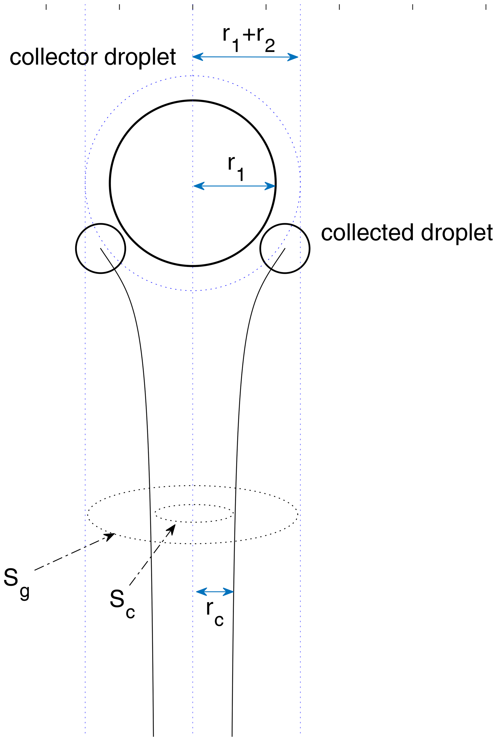
Figure 1A schematic diagram for a droplet pair collision. The initial vertical distance between the center of the two droplets is set to be 30 (r1+r2), which approximates two droplets initially separated by an infinite distance. To calculate the collection cross section , the initial horizontal distance needs to be changed with the bisection method until it converges to rc. Collision happens only when the initial horizontal distance is smaller than rc.
Two droplets may not coalesce even when they collide with each other. Observations show that the droplet pair can rebound in some cases because of an air film temporarily trapped between the two surfaces. Especially for droplets with radii both larger than 100 µm, the coalescence efficiency is remarkably less than 1.0. Beard and Ochs (1984) provide a formula of the coalescence efficiency for a certain range of droplet radii. Basically, the coalescence efficiency is a function of the sizes of the two droplets in their formula.
In this study, electric charges and external electric fields are taken into consideration for droplet collision–coalescence. The droplet distribution function has two variables, namely droplet mass m (or radius r) and electric charge q. The SCE can be expressed as follows:
where is the distribution of the droplet number concentration over mass and charge, and K is the collection kernel of the two classes of droplets. The collection kernel K () represents the rate at which droplets of mass mx and charge qx collide with droplets of mass m−mx and charge q−qx to form new droplets of mass m and charge q.
The collection kernel for charged droplets in an external electric field has the same form as Eq. (2). However, terminal velocity, collision efficiency, and coalescence efficiency in the kernel may all be affected by the electric charge and field. We consider these as electrostatic effects. In a vertical electric field, the terminal velocity of a charged droplet may be increased or decreased, depending on the charge sign and the direction of the field. The threshold horizontal distance rc, the collision cross section, and the collision efficiency of a droplet pair may be changed because the electric charge and field can make the droplets to cross the streamlines more easily under some circumstances. Therefore, terminal velocity, collision efficiency, and coalescence efficiency not only depend on the sizes of the two droplets, but may also depend on the electric charge and the external electric field.
As will be seen in this study, the electrostatic effect on collision efficiency is much stronger than on terminal velocity. Therefore, the electrostatic effect on terminal velocity is presented in Sect. 6 as the discussion, and we focus on the electrostatic effects on collision efficiency in this paper. The method for obtaining droplet terminal velocity and collision efficiency with the electrostatic effects will be presented in Sect. 3. The electrostatic effect on coalescence efficiency is not considered here. The coalescence efficiency used in this study is the same as that for uncharged droplets, based on the results of Beard and Ochs (1984). In their study, coalescence efficiency is a function of r1 and r2 and is valid for 1<r2<30 µm and 50<r1<500 µm. In this study, however, the range of r1 and r2 is much wider – from 2 to 1024 µm. The formula of the coalescence efficiency in Beard and Ochs (1984) is extrapolated for the droplet size range here. The coalescence efficiency is set to be 1 if the extrapolated value is higher than 1 or set to be 0.3 if the extrapolated value is smaller than 0.3.
3.1 Equations of motion for charged droplets
In order to calculate the terminal velocity and collision efficiency, the equations of motion need to be solved. Droplet motion depends on the following three forces: gravity, the flow drag force, and the electrostatic force due to droplet charge and the external electric field. The equations of motion for a pair of droplets are as follows:
where subscripts 1 and 2 denote droplet 1 and droplet 2, respectively, g is the gravitational acceleration, v is the velocity of the droplet relative to the flow if there are no other droplets present, u is the flow velocity field induced by the droplet, μ is the dynamic viscosity of air, C is the drag coefficient, which is a function of Reynolds number, r is the droplet radius, and m is the droplet mass, with , and Fe is the electrostatic force. We set the air temperature at T=283 K and pressure p=900 hPa in this study for the calculation of air dynamic viscosity.
3.2 The drag force term
The flow drag force is described by the second term on the right hand side of Eq. (4), which assumes a simple hydrodynamic interaction of the two droplets. That is, each droplet moves in the flow field induced by the other one moving alone, and it is called the superposition method in cloud physics. This method has been successfully used in many studies for the calculation of collision efficiencies (Pruppacher and Klett, 1997). The superposition method can also ensure that the stream function satisfies the no-slip boundary condition (i.e., Wang et al., 2005). To calculate the flow drag force, the induced flow field u is required. The method for obtaining the induced flow field u is discussed below.
Considering a rigid sphere moving in a viscous fluid with a velocity U relative to the flow, the stream function depends on the Reynolds number of this spherical particle, , where ρ is the density of the air, and μ is the dynamic viscosity of the air. It is known that when the Reynolds number is small, the flow is considered as being a Stokes flow, and the stream function can be expressed as follows:
where is the normalized distance (R is the distance from the sphere center, and r is the droplet radius), θ0 is the angle between the droplet velocity and vector R pointing from the sphere center. U is the value of the droplet velocity relative to the flow, i.e., for droplet 1 and for droplet 2. However, this stream function for the Stokes flow does not apply to the system with a large Reynolds number. Hamielec and Johnson (1962, 1963) gave the stream function ψh induced by a moving rigid sphere, which can be used for flows with large Reynolds numbers as follows:
where are functions only of the Reynolds number NRe for each droplet. The method is valid for NRe<5000. But the solution deviates from the Stokes flow solution when NRe→0 for small droplets. Cloud droplets with radii ranging from 2 to 1024 µm typically have a Reynolds number ranging from 10−4 to 103. Therefore, it is necessary to construct a stream function that applies to a wide range of NRe. This work adopts a stream function that is a linear combination of ψh and a Stokes stream function ψs (Pinsky and Khain, 2000) as follows:
which converges to a Stokes flow when NRe→0. Then the induced flow field u is derived as follows:
where and are the unit vectors in the polar coordinate (R, θ0). It can also be expressed in Cartesian coordinates (x, z) as follows:
where the direction of is vertically down, the same as gravitation. φ is the angle between and the droplet velocity v.
Both the Stokes and Hamielec stream functions satisfy the no-slip boundary condition, i.e., the fluid velocity on the surface of the droplet is equal to the velocity of the droplet. The Hamielec stream function is no-slip because those functions in Eq. (6) satisfy and , as long as the droplet is considered as a rigid sphere (Hamielec, 1963). These relations ensure that at the surface of the droplet, which means the no-slip boundary condition. (Note that uθ is the tangential component of the velocity of the fluid, and Usin θ0 is the tangential velocity of the droplet surface.)
According to an empirical equation of Beard (1976), the drag coefficient C in Eq. (4) is a function of NRe as follows:
where X=ln (NRe) and fitting constants are from Table 1 of Beard (1976). The drag coefficient increases with the Reynolds number. For example, the terminal velocity of a droplet of 2 µm in radius is 4.92 × 10⁻⁴ cm s−1, with NRe=1.23 × 10⁻⁴ and C=1.00001; the terminal velocity of a droplet of 32 µm in radius is 11.8 cm s−1, with NRe=0.47 and C=1.07; the terminal velocity of a droplet of 1024 µm in radius is 715 cm s−1, with NRe=915 and C=18.0.
For droplets with r<10 µm, the assumption of no-slip boundary condition is no longer valid because droplet sizes are comparable with the mean free path of air molecules. Air cannot be considered as a continuous medium. The flow slips on the droplet surface. To take this effect into consideration, the drag coefficient should be multiplied by another coefficient (Lamb and Verlinde, 2011, p. 386) as follows:
where λ is the free path of air molecules, and r is the droplet radius.
3.3 The electric force term
The electric force is described by the third term on the right side of Eq. (4). The electric force includes the interactive force between the two charged droplets, and it is also an external electric force if there is an external electric field. For two point particles, we apply Coulomb's law as follows:
where Fe is the interactive force between point charges q1 and q2, and R is the distance between the two point charges. However, this inverse-square law does not apply to uneven charge distribution such as the case of charged cloud droplets.
The interaction between charged conductors is a complex mathematical problem in physics. Davis (1964) demonstrated an appropriate computational method for an electric force between two spherical conductors in a uniform external field. The electric force depends on droplet radius (r1,r2), charge (q1,q2), center distance R, electric field E0, and the angle θ between the electric field and the line connecting the centers of two droplets (note that ). The resultant electric force acting on droplet 2 is expressed as follows:
where is the radial unit vector, is the tangential unit vector, E0 is the eternal electric field, and parameters F1 to F10 are a series of complicated functions of geometric parameters (; Davis, 1964).
The electric force directly from the external field is shown as two terms in Eq. (13) and can be simply written as E0q2 if the two terms are combined. The second half of Eq. (13) represents the interactive force from droplet 1 in the radial direction and tangential direction, respectively. Note that the third term represents the interactive force from droplet 1 if there is no external electric field. Except for this term, all the other terms in Eq. (13) are the interactive forces from droplet 1 due the induction from the external field.
Similarly, the resultant electric force Fe1 acting on droplet 1 includes both the force directly from the external field and the interactive force from droplet 2. The sum of the electric forces on the two droplets, Fe1+Fe2, must equal to the external electric force acting on the system, which can be expressed as E0(q1+q2), because the two droplets can be considered as a system. Then, the electric force acting on droplet 1 can be derived immediately as follows:
Figure 2 is a schematic diagram showing the forces acting on each droplet in a pair. Also shown in Fig. 2 is the velocity of each droplet relative to the flow, if there are no other droplets present (v), and the flow velocity induced by the other droplet (u). Droplet velocity relative to the flow is v−u. The electric field E0 is in the downward direction, which is the same as gravity. Droplet 1 has a positive charge and droplet 2 has a negative charge in this example. The forces acting on each droplet include gravity, flow drag force, and the electrostatic force, as seen on the right side of Eq. (4). For droplet 1, the electric force directly from the external field is in the downward direction and is shown as E0q1 in the figure. The interactive electric force from droplet 2, shown as Finter in the figure, has a radial component and a tangential component, so that it is in a direction that does not necessarily align with the line connecting the two droplets. Because of the interactive electric force from droplet 2, the velocity v of droplet 1 is not in the vertical direction. The electrostatic force between charged droplets tends to make the droplets attract each other. This force is particularly strong when droplets are close to each other, thus enhancing collisions. The flow drag force on droplet 1 is in the opposite direction with v−u.
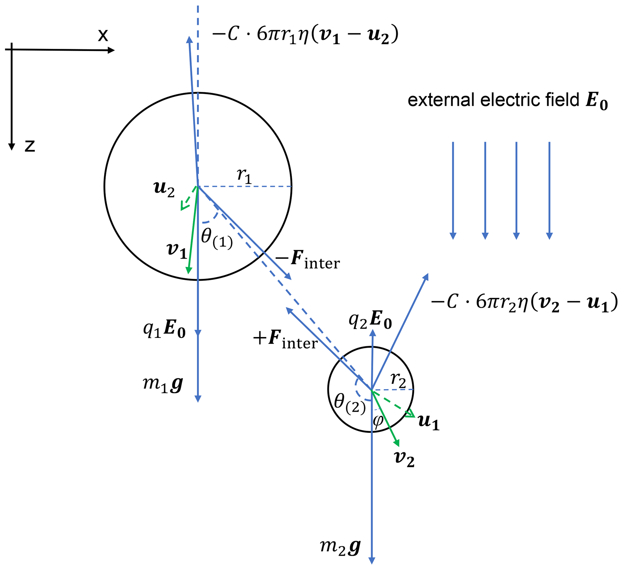
Figure 2A schematic diagram of all the forces acting on two charged droplets and droplet velocities and the induced flow velocities. The electric field E0 is vertically downward, and the electric charges are q1>0,q2<0. Note that the electrostatic force Fe1, Fe2 includes two parts, namely the electric force from the other droplet (Finter in the figure) and the force purely from the external electric field (q1E0, q2E0 in the figure).
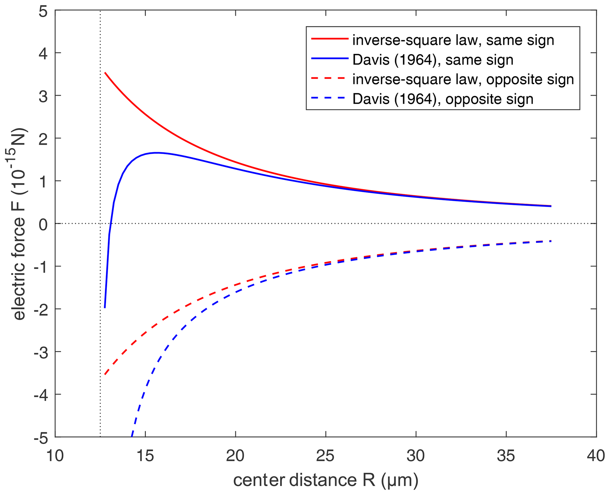
Figure 3Comparison of the electric force from the conductor model (Davis, 1964; Eq. 15 in this study) and the inverse-square law (Eq. 12 in this study). Positive force represents repulsion and negative force represents attraction. Radius of the pair is set to r1=10 µm and r2=2.5 µm, respectively. Solid lines are for the droplet pair with the same sign of electric charges, with and . Dashed lines are for droplets with the opposite sign of electric charges, with and .
If there is no external electric field but only a charge effect, Eq. (13) is reduced to the following:
To illustrate it, a comparison between the electrostatic forces derived by the inverse-square law and conductor model without electric field (i.e., Eq. 15) is shown in Fig. 3, where the electric force between droplets with opposite-sign charges (dashed lines) and with same-sign charges (solid lines) varies with distance. When , we have , and it is also shown that two models are basically identical in remote distance. But when the spheres approach closely, the conductor interaction (blue lines) changes to strong attraction, because of electrostatic induction. The interaction is always attraction at a small distance, regardless of the sign of charges. If there is only an inverse-square law without electrostatic induction, it is obvious that the same-sign charges must decrease collision efficiency. However, after taking electrostatic induction into account, the effects of same-sign and opposite-sign charges need to be reconsidered.
3.4 Terminal velocity and collision efficiency
The equations of motion (Eq. 4), along with the other equations in this section, are used to calculate the terminal velocities of charged droplets. Note that the terminal velocity refers to the steady-state velocity of a droplet relative to the flow when there are no other droplets present, as mentioned earlier. Therefore, by setting the induced flow u to be 0, Eq. (4) can be integrated to obtain the terminal velocity of the droplets with electric charge and field.
Equation (4), along with other equations, is also integrated to obtain the trajectories for the two droplets in any possible droplet pair (r1,q1 and r2,q2) for different strengths of the downward electric field (0, 200, and 400 V cm−1). The second-order Runge–Kutta method is used for the integration. The initial settings of droplet positions and velocities and the flow velocities are required. To save computational power, the initial vertical distance is set to be 30 (r1+r2), as an approximation of infinity. The initial flow velocity field u1 and u2 are set to be zero. Initial velocities of the two droplets are set to be the terminal velocities V1 and V2. We vary the initial horizontal distance using the bisection method until we find a threshold distance rc, which is the maximum horizontal distance at which the two droplets can collide. The threshold distance is found with a precision of 0.1 %. The collision cross section and collision efficiency E are than calculated.
After computing the collision efficiencies E for a droplet pair with (r1,q1) and (r2,q2), the collection kernel is then derived. With the collection kernel , the effect of the electric charges and fields on the droplet collision is determined by solving the SCE.
4.1 Setting of the bins for droplet radius and charge
To solve the stochastic collection equation (Eq. 3) numerically, droplet radius and charge are both divided into discrete bins that are logarithmically equidistant. Droplet radius, ranging from 2 to 1024 µm, is divided into 37 bins, with the radius increasing by a factor of 21∕4 from one bin to the next. Droplets with radii larger than 1024 µm are assumed to precipitate out and are not included in the size distribution.
In each radius bin, droplets may have different amounts and different signs of charges. For the bin of radius r, droplet charge ranges from −32 r2 to +32 r2 (in units of elementary charge and r in µm). This means that smaller droplets have a smaller range of charge. The setting here is based on the observations that the charge amount is proportional to the square of droplet radius, as discussed in the Introduction. The upper limit charge bin of 32 r2 is close to the thunderstorm condition of 42 r2. The charge range is then divided into 15 bins, with the center bin having zero charge, seven bins to the right having positive charges, and seven bins to the left having negative charges. For the positive charge bins, the one next to the center bin has a charge of +0.5 r2. The charge amount is increased by a factor of 2 from this bin to the next, until the upper limit of 32 r2 is reached. The setting for the negative charge bins is symmetric to the positive charge bins. For the size bins and charge bins described above, a large matrix of kernel is computed in advance as a lookup table for solving the SCE.
4.2 Redistribution of droplets into radius and charge bins after collision–coalescence
Droplet size and charge after collision–coalescence usually do not fall into any existing bins. A simple method is to linearly redistribute the droplets to the two neighboring bins (Khain et al., 2004). We first redistribute the droplets to the size bins. The ratio of redistribution is simultaneously based on total mass conservation and droplet number conservation. For example, to redistribute droplets with mass m (mi<m<mi+1) and number Δn, a proportion of is added to the ith bin, and is added to the (i+1)th bin. These droplets are then redistributed to the charge bins within each size bin, satisfying the total charge conservation and droplet number conservation. For example, to redistribute droplets with charge q () within the ith size bin, a proportion of is added to the bin of (i,j), and a proportion of is added to the bin of (1).
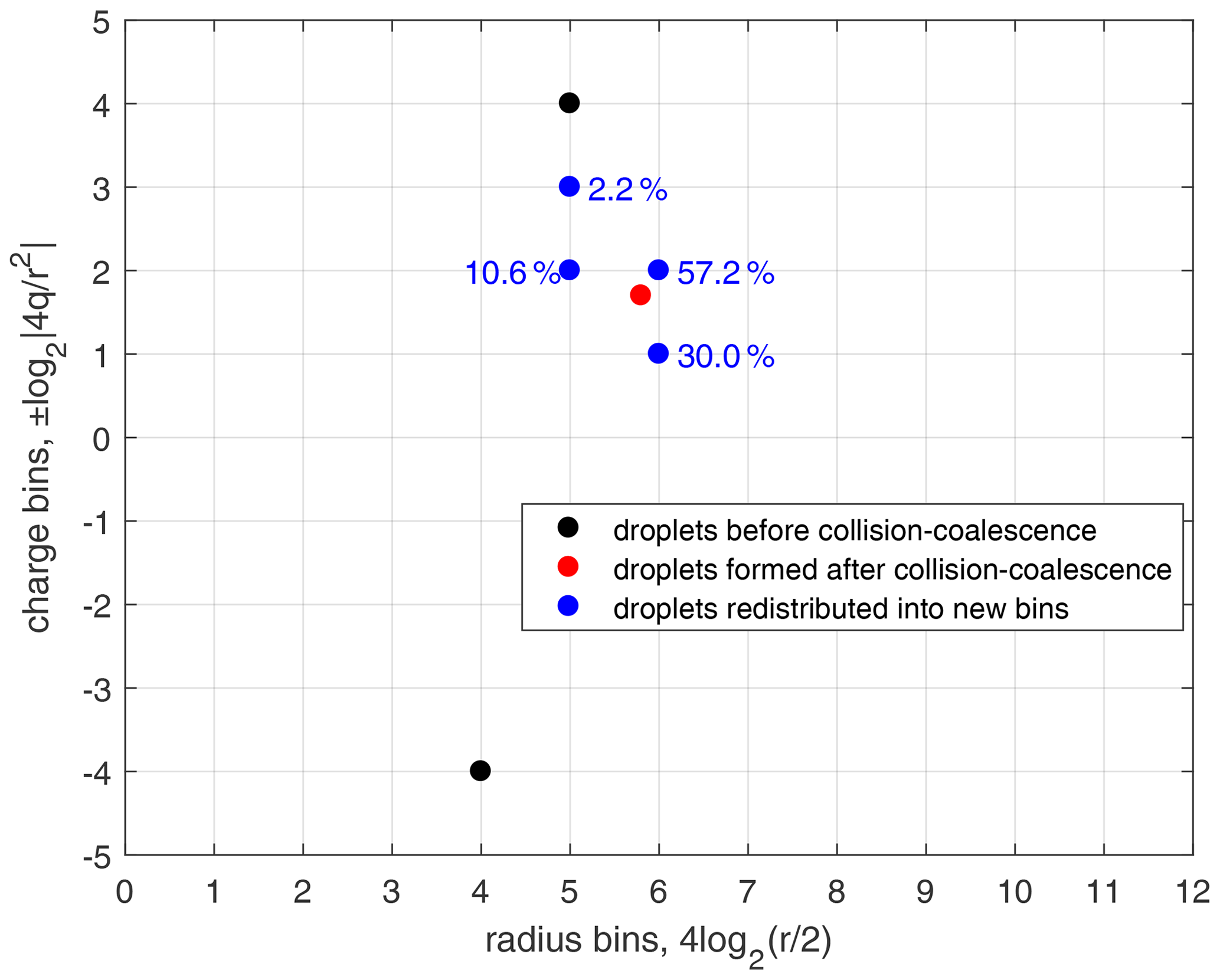
Figure 4An example of droplet redistribution to new size and charge bins after collision–coalescence. Black dots denote the two bins of droplets before collision–coalescence. The red dot denotes the droplets after collision–coalescence but not on the bin grids. Blue dots denote the droplets that are redistributed to the new bins. Numbers close to the blue dots are the percentage of droplets that are redistributed into that bin. The redistribution method is constrained by particle number conservation, mass conservation, and charge conservation.
As shown in Fig. 4, the collision–coalescence between bin (r1,q1) and bin (r2,q2), shown with black dots, generates droplets shown with the red dot. These newly generated droplets are then redistributed into two size bins and are further redistributed into two charge bins within each of the size bins, as shown with the blue dots. Note that the numbers close to each of the blue dots in Fig. 4 are the percentages of droplets that are redistributed into that bin. In fact, this method only reaches first-order accuracy. Although Bott (1998) compared several methods for redistributing droplets with higher-order correction, the two-parameter distribution is too complicated to do the higher-order correction in this study.
4.3 The initial droplet size and charge distributions
The initial droplet size distribution used in this study is derived based on an exponential function in Bott (1998) as follows:
where n(m) is the distribution of droplet number concentration over droplet mass, L is the liquid water content, and is the mean mass of droplets. This function is used to derive n(ln (r)), which is the distribution of droplet number concentration over droplet radius. With the definitions of n(m) and n(ln (r)), and , where ρ is droplet density, we can derive n(ln (r)) as follows:
By substituting Eq. (16) into Eq. (17) and assuming that , where is the mean radius, we have the following:
Equation (18) is used as the initial droplet size distribution for the calculations of collision–coalescence in this study. It has two parameters, L and , and can be considered as a gamma distribution. Using parameters L and in the initial size distribution has the advantage of representing the aerosol effect. The parameter L can be set as a constant. Using a different mean radius can represent different aerosol conditions and a different number concentration of cloud droplets.
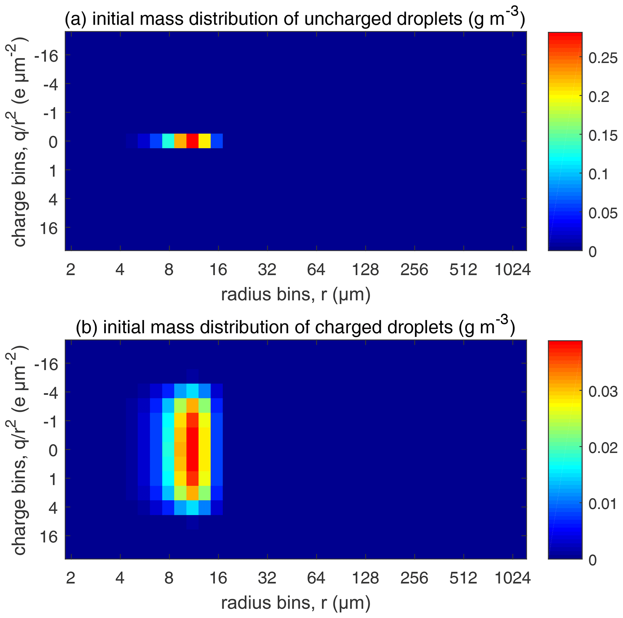
Figure 5The initial droplet mass distributed over the size and charge bins. Colors represent water mass content in the bins (in units of g m−3). (a) Uncharged droplets and (b) charged droplets.
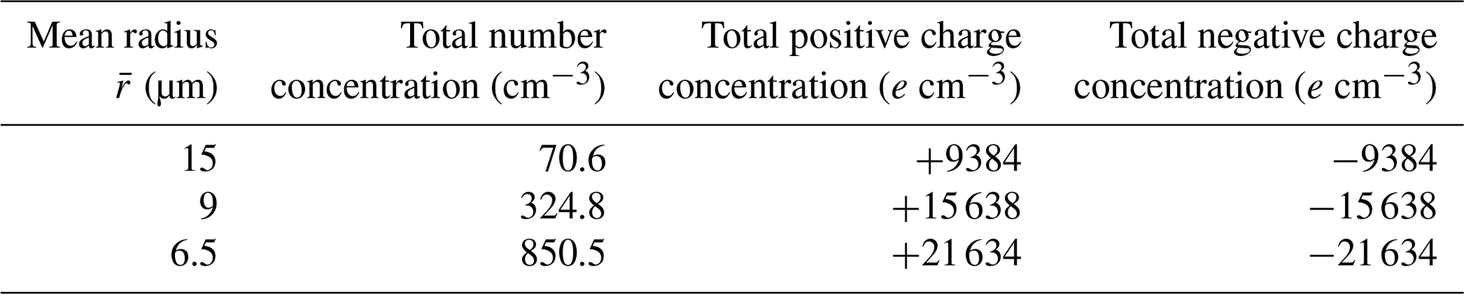
A total of 12 cases with different initial conditions are considered for studying the evolution of droplet distribution. The mean droplet radius is set with three different sizes, namely 15, 9, and 6.5 µm, where µm case represents clean conditions and 6.5 µm represents polluted conditions. The liquid water content in our study is set at L=1 g m−3, which is a typical value in warm clouds, according to observations (Warner, 1955; Miles et al., 2000). With the fixed liquid water content, a smaller mean radius corresponds to a larger number concentration. As shown in Table 1, , 9, and 6.5 µm give an initial droplet number concentration of 71, 325, and 851 cm−3, respectively.
Table 1Total number concentration and charge content for all initial droplet distributions.
For each , comparisons are made among four different electric conditions in which (a) droplets are uncharged, (b) droplets are charged but have no external electric field, (c) droplets are charged and also have an external downward electric field of 200 V cm−1, and (d) droplets are charged and also have an external downward electric field of 400 V cm−1. For the uncharged cloud, the initial distribution is shown in Fig. 5a, where all droplets are put in the bins with no charge. For the charged clouds, an initial charge distribution shown in Fig. 5b is made as follows. To simulate an early stage of the warm cloud precipitation, we need to distribute the droplets in each size bin to different charge bins so that these droplets have different charges. Since there is little data on this, we assume a Gaussian distribution as follows:
where N0 is the number concentration in the size bin, and σ is the standard deviation of the Gaussian distribution in that size bin. N(q) represents the number concentration of droplets with charge q. This distribution satisfies electric neutrality . For different size bins, the droplet number concentration N0 is different. We purposely set the standard deviation σ to be different for different size bins. For a larger size, the charge amount is larger, based on r2 (q in units of elementary charge and r in µm) as stated in the Introduction. Therefore, we set a larger standard deviation σ for the larger size bins. With this setting of droplet charge, the total amount of charge in each case is shown in Table 1. The , 9, and 6.5 µm cases have an initial charge concentration of 9438, 15 638, and 21 634e cm−3, respectively, for both positive charge and negative charge.
The initial electric charges and electric field strength are set according to the conditions in warm clouds or in the early stage of thunderstorms. In fact, in some extreme thunderstorm cases, both the electric charge and field could be 1 order of magnitude larger (Takahashi, 1973) than the values used in this study. Furthermore, in natural clouds, the electric charge on a droplet leaks away gradually. In this study, the charge leakage is assumed to be a process of exponential decay (Pruppacher and Klett, 1997), and the relaxation time is set to τ=120 min. Thus, all the bins lose of electric charge in each time step of Δt=1 s.
5.1 Collision efficiency
Here we present collision efficiencies for typical droplet pairs to illustrate the electrostatic effects. During the evolution of droplet size distribution, the radius and charge amount of colliding droplets have large variability. In addition, the charge sign of the colliding droplets may be the same or the opposite. Therefore, only some examples are shown.
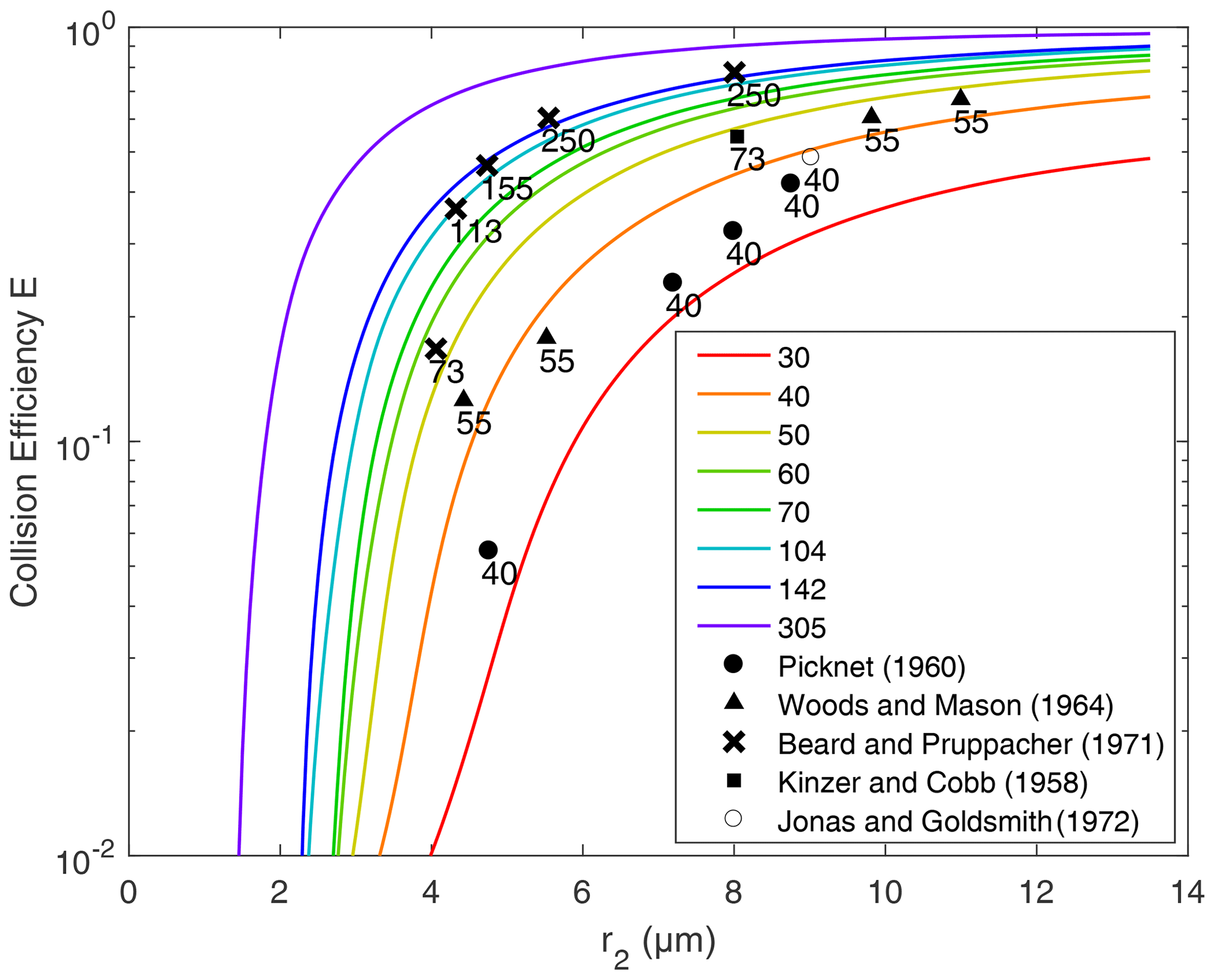
Figure 6Collision efficiency for droplets with no electric charge or field. Lines are the results computed in this study. Different lines represent the different collector radius r1, from 30 to 305 µm. The x axis denotes the collected droplet radius r2. Scatter points represent the collision efficiencies from previous experimental studies. The numbers next to these points represent the collector drop radius.
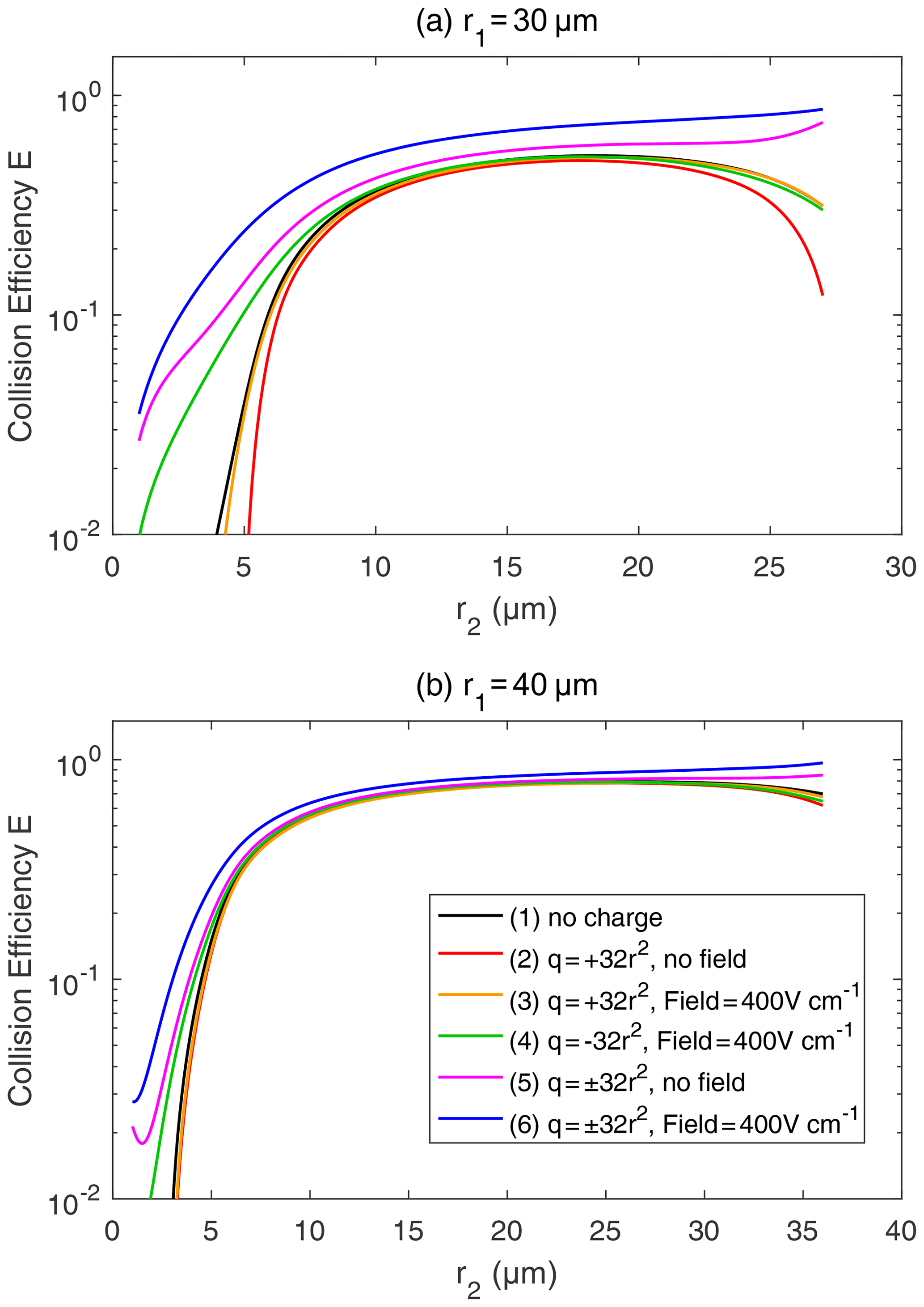
Figure 7Collision efficiency for droplets with electric charge and field. The radius of the collector droplet r1 is (a) 30.0 µm and (b) 40.0 µm. The x axis denotes the collected droplet radius r2. The two droplets carry electric charges proportional to r2. In both panels, line (1) for droplet pairs with no charge is the same as the 30 and 40 µm lines in Fig. 6. In line (1), the setting of the electric charge and field is no charge and no field. Line (2) shows and , with no field. Line (3) shows and , with a downward electric field of 400 V cm−1. Line (4) shows and , with a downward electric field of 400 V cm−1. Line (5) shows and , with no field. Line (6) shows and , with a downward electric field of 400 V cm−1.
The collision efficiencies for droplet pairs with no electric charge and field are presented in Fig. 6 as a reference. Collector droplets with radii larger than 30 µm are shown here to represent the precipitating droplets. The calculated collision efficiencies from this study are also compared with the measurements from previous studies. It is seen that results from this study are generally consistent with the measurements. Collision efficiencies increase as r2 changes from 2 to 14 µm and also increase as r1 changes from 30 to 305 µm. For two droplets that are both large enough, the collision efficiency could be close to one.
Figure 7 shows the collision efficiencies for droplet pairs with electric charge and field. Basically, droplet pairs that have no charge, same-sign charges, and opposite-sign charges are selected here and under the 0 and 400 V m−1 electric fields. Results for the collector droplet with a radius of 30 µm (Fig. 7a) and 40 µm (Fig. 7b) are shown. When comparing Fig. 7a and b, it can be seen that electrostatic effects are less significant for a larger collector. The electrostatic effects are even weaker for a collector radius larger than 40 µm (figures not shown). Therefore, we use the 30 µm collector as an example to explain the electrostatic effects on collision efficiencies below.
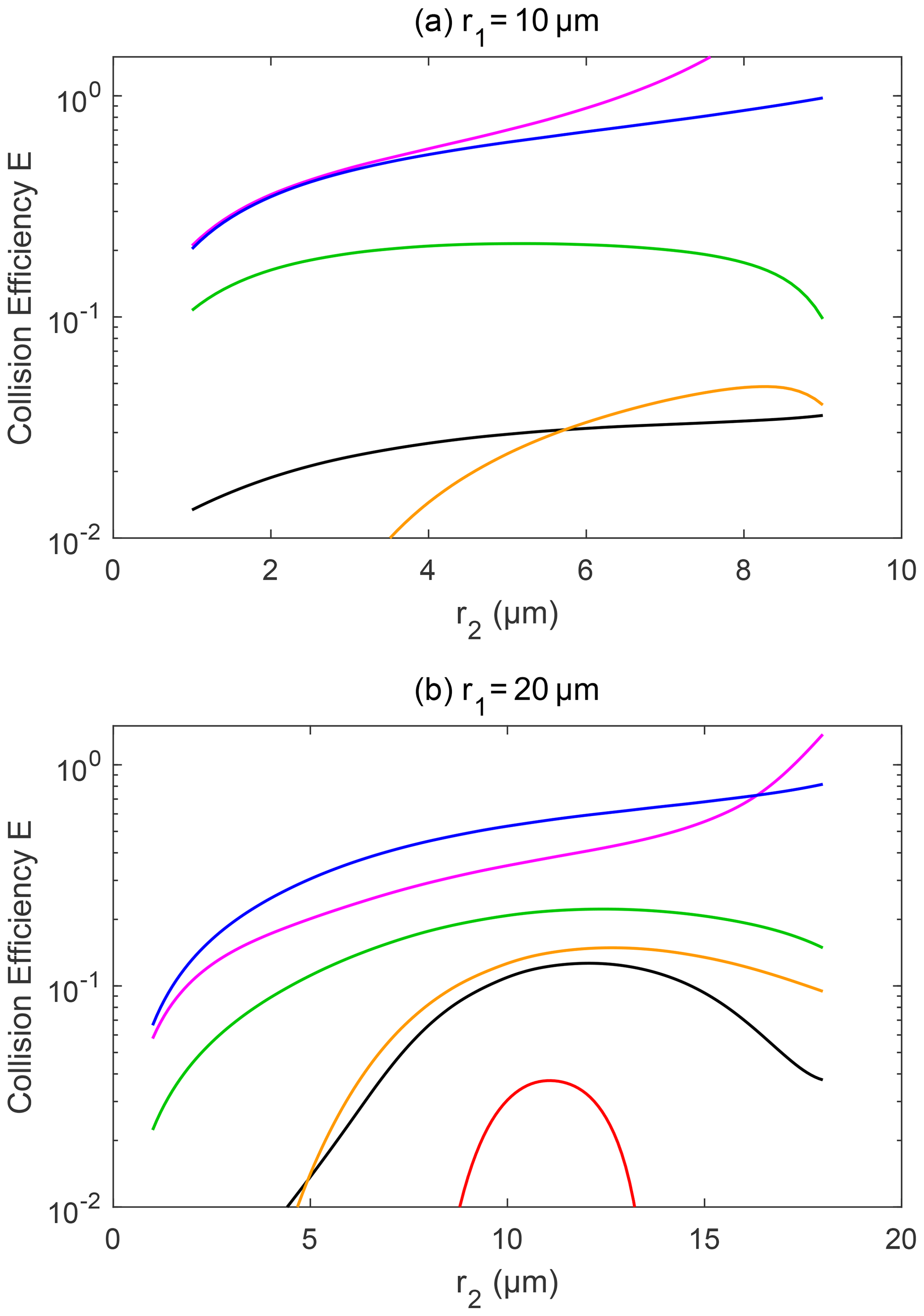
Figure 8Collision efficiency for droplets with electric charge and field. The radius of the collector droplet r1 is (a) 10.0 µm and (b) 20.0 µm. The other characteristics of the droplet pairs are similar to those in Fig. 7.
For the collector droplet with a radius of 30 µm (Fig. 7a), a noticeable, and sometimes significant, electrostatic effect can be seen. Compared to the droplet pair with no charge (line 1), the positively charged pair under no electric field (line 2) has a slightly smaller collision efficiency due to the repulsive force. As can be seen in Fig. 3, when the charged droplets move together, they first experience a repulsive force and then an attractive force at a small distance. The net effect is that the droplets have a smaller collision efficiency. The results for negatively charged pair under no electric field are identical to line 2 and are therefore not shown. When a downward electric field of 400 V m−1 is added, the positively charged pair (line 3) has a collision efficiency very close to the pair with no charge. This implies that the enhancement of collision efficiency by the electric field offsets the repulsive force effect. For a negatively charged pair in a downward electric field (line 4), the collision efficiency with a small r2 is significantly enhanced. This could be easily explained by electrostatic induction, i.e., the strong downward electric field induces a positive charge on the lower part of the collector droplet (even though it is negatively charged overall), so the negatively charged collected droplet below experiences an attractive force. In other words, we can approximately consider the collected droplet as a negative monopole (since it is very small) and consider the collector as a negative monopole plus a downward dipole that is induced by the electric field. When the two droplets are relativity far, the monopole–monopole interaction is dominant so that the force is repulsive. But when the two droplets come close, the monopole–dipole interaction becomes dominant in certain circumstances, so the force changes to attractive.
As for a pair with opposite-sign charges, line 5 in Fig. 7a shows that the collision efficiency is enhanced by the electrostatic effect even when there is no electric field. The collision efficiency is nearly 1 order of magnitude higher, with r2<5 µm. Line 6 in Fig. 7a shows that, with an electric field of 400 V cm−1, the electrostatic effect for the pairs with opposite-sign charges is even stronger. There is also an interesting feature in Fig. 7a; as the collector and collected droplets have similar sizes, the collision efficiency is high for the pairs with opposite-sign charges. This is quite different from the other four lines, where collision efficiencies are very low for droplet pairs with similar sizes.
Figure 8 shows the collision efficiencies for droplet pairs with charge and field and with smaller collectors. The collector droplet has a radius of 10 µm (Fig. 8a) and 20 µm (Fig. 8b) here. Collision efficiencies for these smaller collectors are much smaller than one when there is no charge (line 1 in Fig. 8a and b), which is already well known in the cloud physics community. However, the electrostatic effects are so strong that the collision efficiencies could be significantly changed for these collectors. For the collector droplet with a radius of 10 µm (Fig. 8a), the positively charged pair has a very small collision efficiency that is out of the scale in the figure, due to the dominating effect of the repulsive force, as discussed above. For the positively charged pair under a downward electric field, the collision efficiencies have a similar order of magnitude to the pair with no charge. For the negatively charged pair under the downward electric field, and for the pairs with opposite-sign charges, the electrostatic effects are very strong. The negatively charged pair even exhibits collision efficiency increases of as much as 2 orders of magnitude. Similarly, for the collector droplet with a radius of 20 µm (Fig. 8b), the electrostatic effect can lead to 1 order of magnitude increase in collision efficiencies.
It is evident that droplet charge and field can significantly affect the collision efficiency, especially for smaller collectors. This means that the electrostatic effects depend on the radius of collector droplets, and it mainly affects small droplets. The section below provides a detailed description on how these electrostatic effects can influence droplet size distributions.
5.2 Evolution of droplet size distribution
This section shows the electrostatic effects on the evolution of different droplet size distributions. As discussed in Sect. 4, this study uses three initial size distributions, where , 9, and 6.5 µm, respectively. For each initial size distribution, comparisons are made among four different electric conditions, namely uncharged droplets, charged droplets without electric field, charged droplets with a 200 V cm−1 electric field, and charged droplets with a 400 V cm−1 electric field. Note that charged droplets here refers to the initial charge distribution shown in Fig. 5. We also compare the results of the uncharged clouds with , 9, and 6.5 µm, which represent the aerosol effects, and then investigate whether the electrostatic effects can mitigate the aerosol effects during the collision–coalescence process.

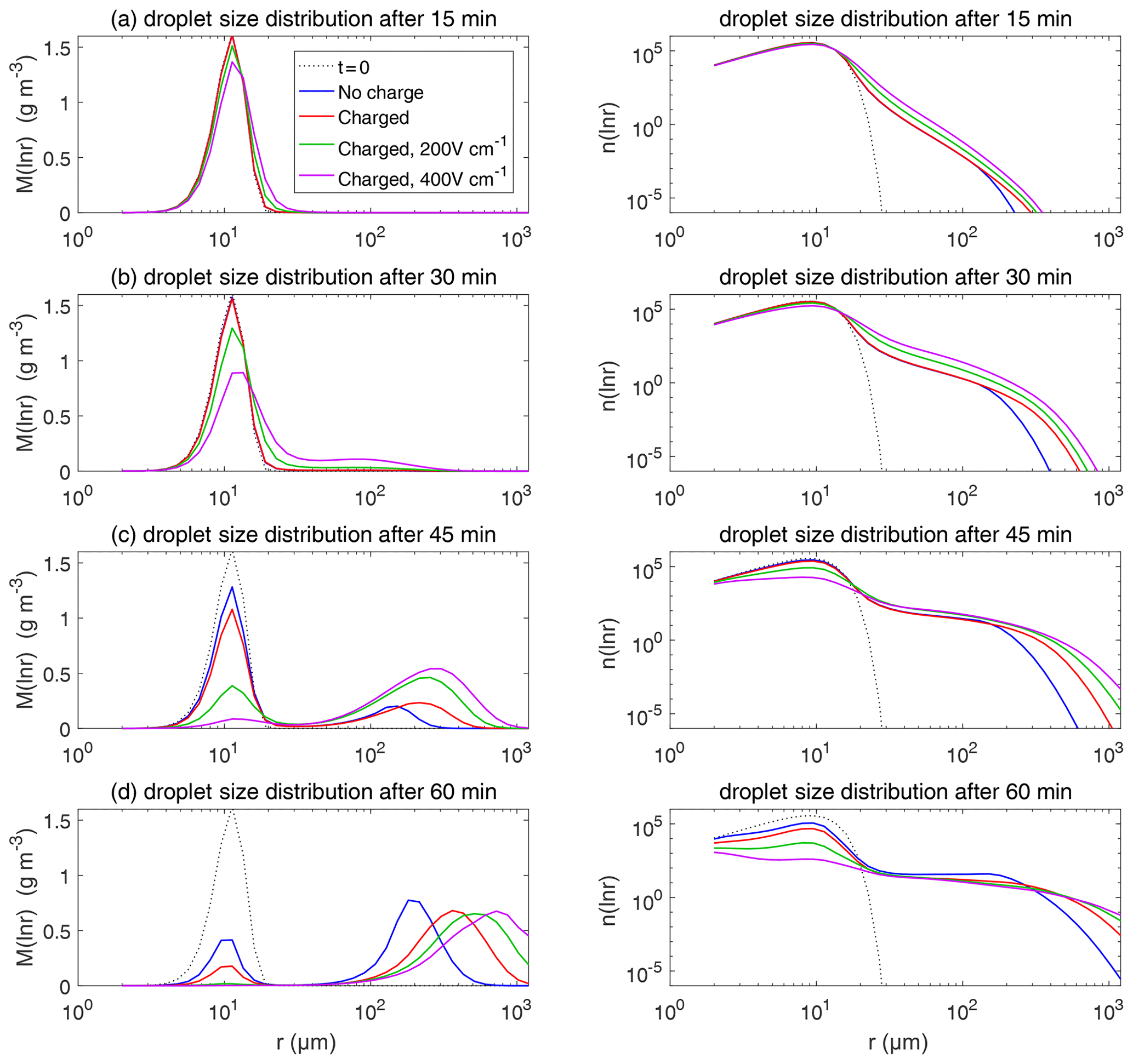
Figure 9The evolution of droplet size distribution with initial µm. These panels show the different stages of the evolution from top to bottom. The left column shows the size distribution of the droplet mass concentration, and the right column shows the size distribution of the droplet number concentration on logarithmic scales. In each panel, comparisons are made for four different electric conditions. Blue lines denote the uncharged cloud. Red lines denote the charged cloud without an electric field. Green and purple lines denote the charged cloud with a field of 200 and 400 V cm−1, respectively. Dotted lines show the initial size distribution.
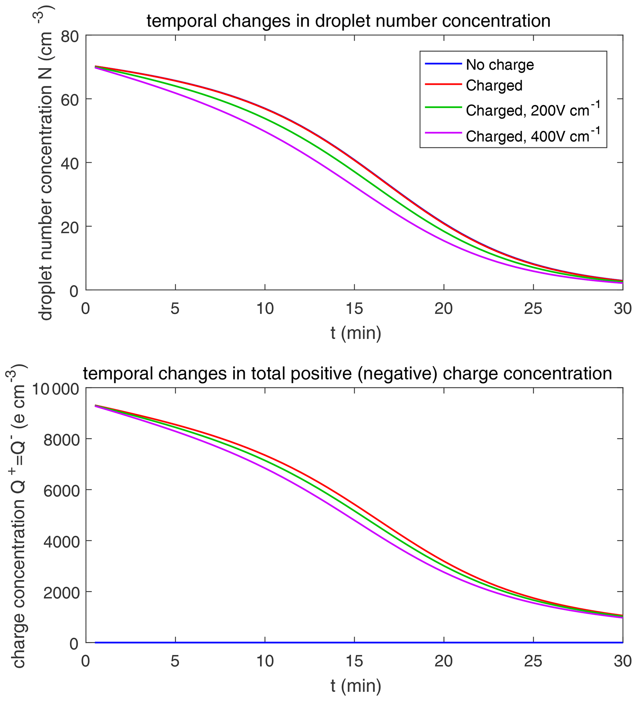
Figure 10Temporal changes in droplet total number concentration and total charge content for µm.
Figure 9 shows the evolution of the droplet size distribution with initial µm, which has an initial droplet number concentration of 71 cm−3. The four rows show different times (t=7.5, 15, 22.5, and 30 min) during the simulated evolution. The left column shows the size distribution of droplet mass concentration M(ln r), and the right column shows the size distribution of droplet number concentration n(ln r). They are related as M(ln r) . A second mode in size distribution gradually forms as droplets undergo the collision–coalescence process from t=7.5 to 30 min. Although the second mode can clearly be seen in the plots of n(ln r), we show M(ln r) here so that the second mode can be seen as a peak. In each panel, the dotted line denotes the initial size distribution (t=0 min) for reference. It is seen that droplet size distributions under four electric conditions have a similar behavior for initial µm in that they all evolve to a double-peak form, regardless of the electric charge or field. At 30 min, the four cases all have a modal radius of about 200 µm (Fig. 9d). The electrostatic effect is not notable for large droplets in the µm cases because the initial radius is large enough to start gravitational collision–coalescence quickly.
The evolution of droplet total number concentration and total positive charge concentration (also equal to the total negative charge concentration) is shown in Fig. 10. It is evident that droplet total number concentration decreases from 71 to less than 5 cm−3 in 30 min and is nearly not affected by the four different electric conditions. Both the positive charge and negative charge concentration decrease from 9384 to about 1000e cm−3 as droplets with opposite-sign charges go through collision–coalescence and charge neutrality occurs.
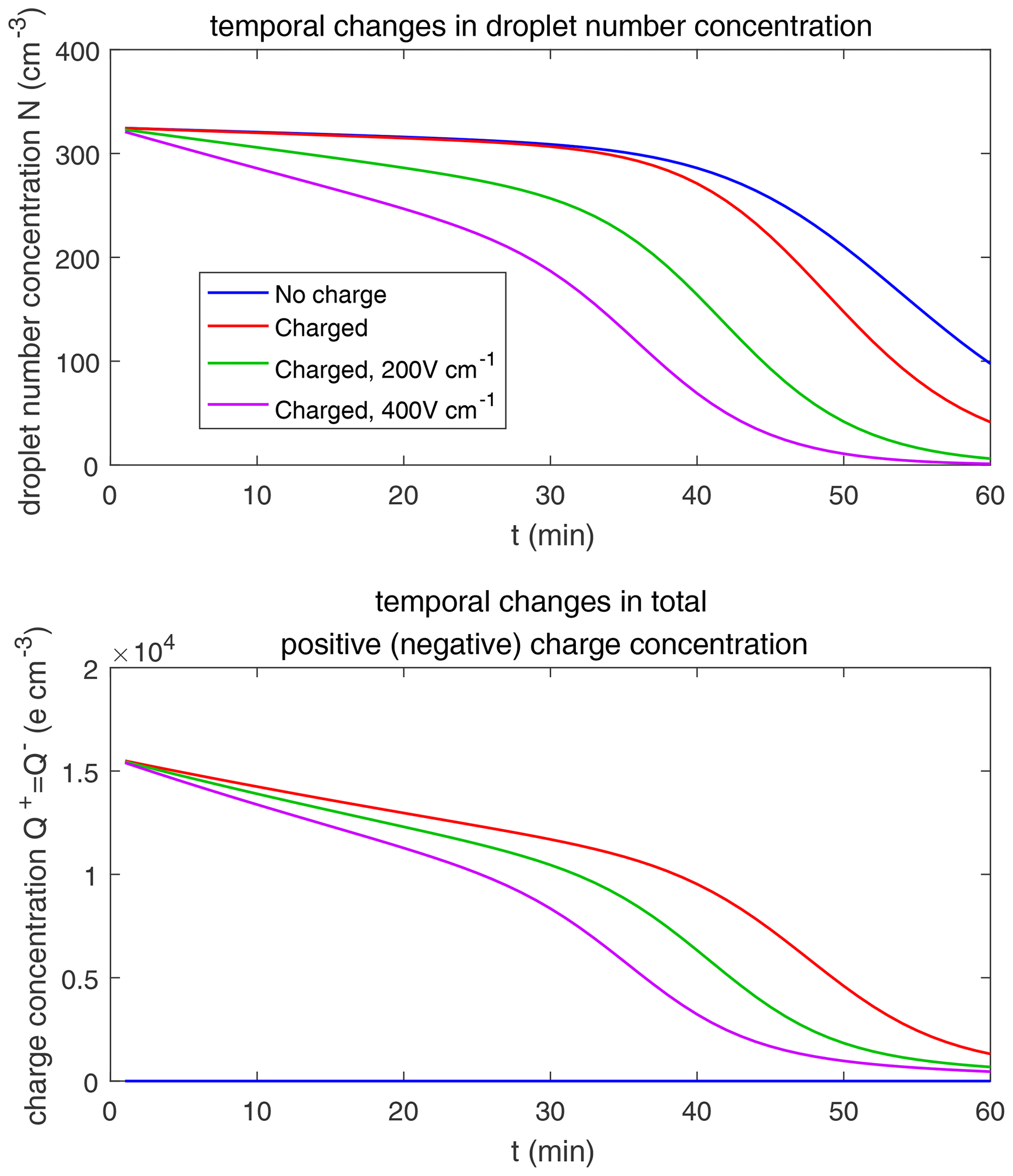
Figure 12Temporal changes in droplet total number concentration and total charge content for µm.
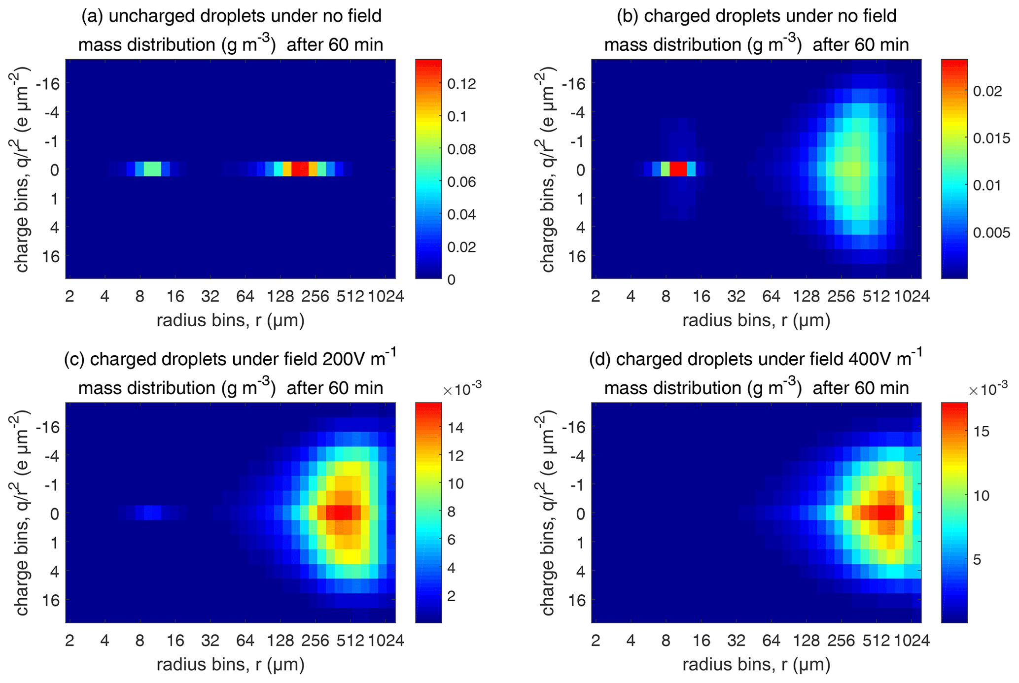
Figure 13Comparison of evolutions of the 2D distribution of droplet mass concentration with different electric conditions at 60 min (initial µm).
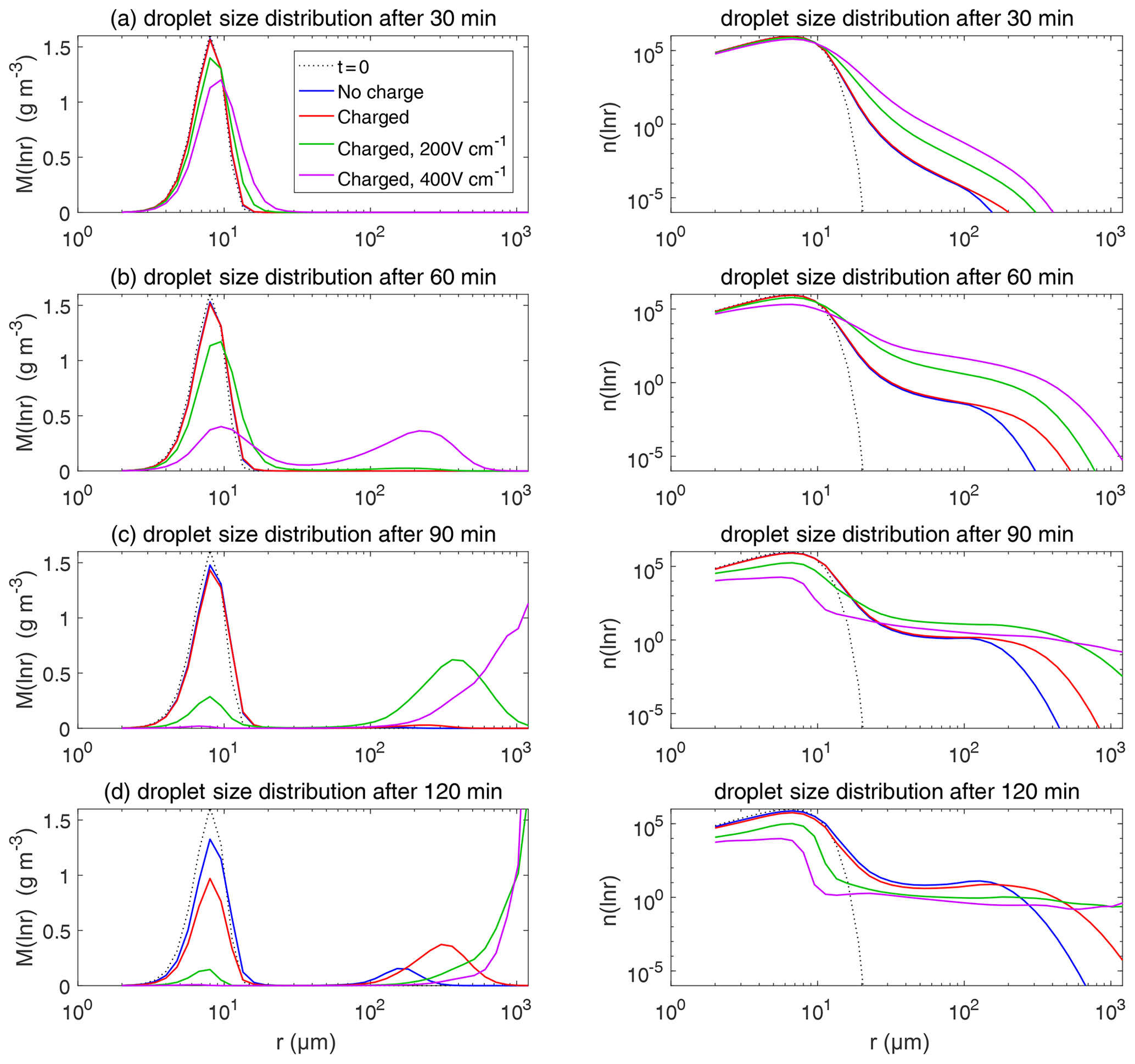
Figure 11 shows the evolution of the droplet size distribution with initial µm. For the uncharged cloud, it takes 60 min to have the second peak grow to about 200 µm. Therefore, the four panels of Fig. 11 show the simulated evolution for t=15, 30, 45, and 60 min. The charges and the electric fields have a more significant effect in the µm case than in the µm case. It is seen that, at 15 and 30 min, the clouds with different electric conditions evidently differ from each other, but the second mode is not obvious. At 45 min, the electrostatic effects on the second peak are evident. The charged cloud (red line) evolves more quickly than the uncharged cloud, as can been from the lower first peak and the growing second peak. Moreover, the downward electric fields further boost the collision–coalescence process of charged droplets (green and purple lines). At 60 min, the modal radius of the second peak is about 200 µm for the uncharged cloud, 300 µm for the charged cloud without an electric field, 500 µm for the charged cloud with a field of 200 V cm−1, and 700 µm for the charged cloud with a field of 400 V cm−1, respectively.
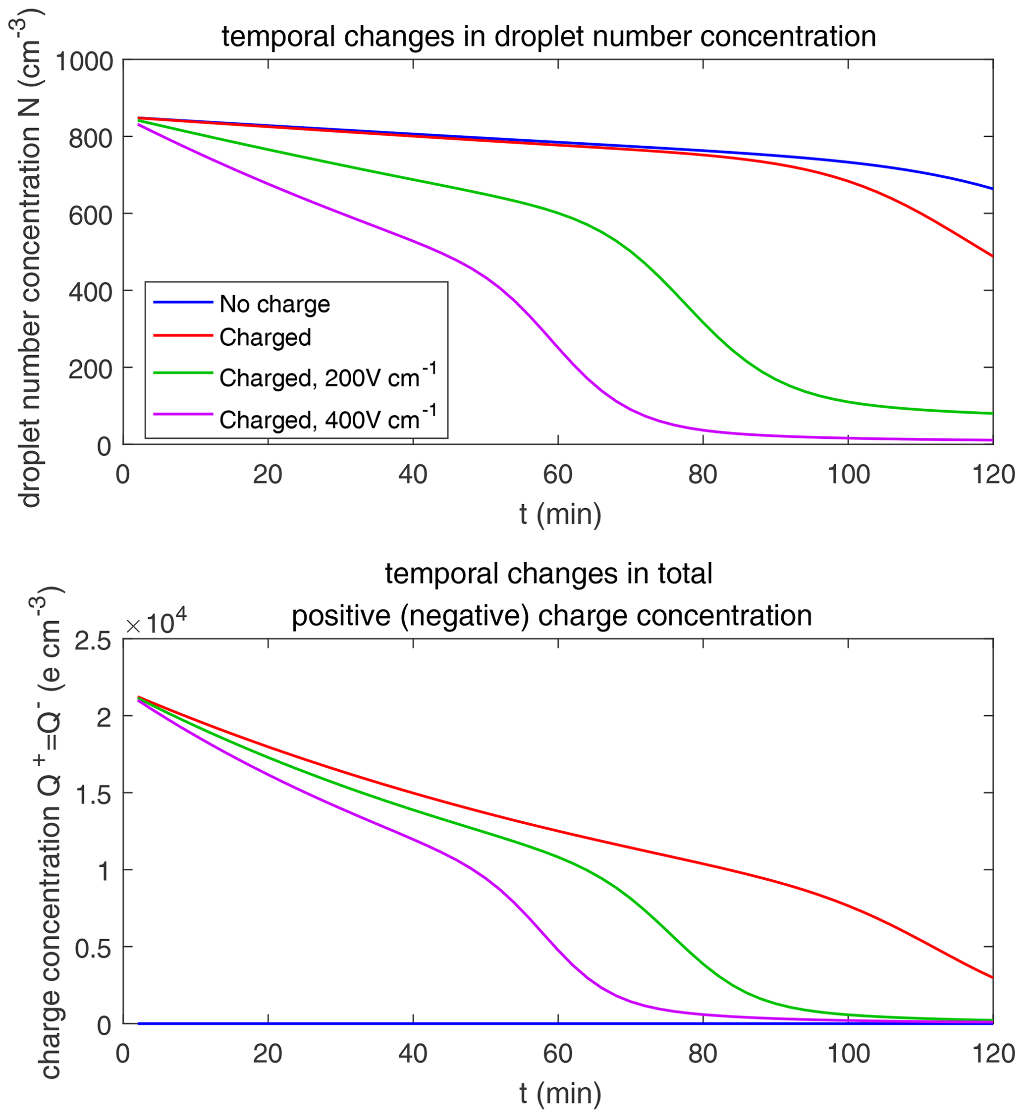
Figure 15Temporal changes in droplet total number concentration and total charge content for µm.
As for the evolution of the droplet total number concentration and charge concentration, Fig. 12 shows that they are distinctly affected by the four different electric conditions. The charged cloud with a field of 400 V cm−1 has a very low droplet number concentration and charge concentration at 60 min. The electrostatic effects play an important role in converting smaller droplets to larger droplets. The 2D distribution of droplet mass concentration for µm at 60 min is shown in Fig. 13. Figure 13a shows the uncharged situation. Figure 13b, c, and d show the situations with charges and with electric fields of 0, 200, 400 V cm−1, respectively. After 60 min of evolution, the distribution of mass over the charge bins is still symmetric. It is also shown that both mass and charges are transported from smaller droplets to larger droplets during collision–coalescence. Note that the integration of this 2D distribution along the charge bins gives a 1D distribution over the droplet size at 60 min, as shown in Fig. 11d.
Figure 14 shows the evolution of the droplet size distribution with initial µm. For the uncharged cloud, it takes 120 min to have the second peak grow to about 200 µm. Therefore, the four panels of Fig. 14 show the simulated evolution for t=30, 60, 90 and 120 min. The enhancement by the electric field on the collision–coalescence process is much more obvious than µm. After 90 min of evolution, the uncharged cloud (blue line) and charged cloud without a field (red line) are almost the same as the initial distribution. This is because the droplets are too small to initiate gravitational collision. At 120 min, a second peak has formed for the situations with no charge and with charge but no field. In contrast, under the external electric field of 200 and 400 V cm−1 (green and purple lines), the cloud droplets grow much more quickly than in the no-field situations. Some droplets have even evolved to larger than 1024 µm, which are supposed to precipitate out from the clouds. The evolution of droplet total number concentration and charge concentration is shown in Fig. 15, which indicates that droplet total number concentrations and charge concentration are strongly affected by the electrostatic effects. These results show that, the electric field would remarkably trigger the collision–coalescence process for the small droplets.
As for the initial mean droplet radius µm (figure not shown), similar to Fig. 14, the droplet size distribution of uncharged and charged clouds without electric field would have nearly no difference, while the effect of electric fields is much stronger. This means that the charge effect is relatively small compared to the electric fields when the initial droplet radius of the cloud is small enough.
Now we compare the electrostatic effects shown above with the aerosol effects. Let us take the cases with µm and µm as examples. When there are no electrostatic effects, the case with µm can develop a significant second peak in the size distribution in less than 30 min, while it takes about 60 min for the µm case to develop a similar second peak, as can be seen in Figs. 9 and 11. This can be regarded as an aerosol effect. When considering the electrostatic effects, it only takes about 45 min for the µm case to develop a similar second peak, as can be seen in Fig. 9. Therefore, the aerosol-induced precipitation suppression effect is mitigated by the electrostatic effects.
According to Eq. (2), the collection kernel K is composed of the collision efficiency E, relative terminal velocity, and coalescence efficiency ε. It is found that the total electrostatic effect on K is mainly contributed by E. The relative terminal velocity term also contributes to the collection kernel K. As mentioned in Sect. 3.4, terminal velocities V1 or V2 are derived by simulating just a single charged droplet in the air with a certain electric field and letting it fall until its velocity converges to the terminal velocity. Therefore, the electric field can affect the terminal velocities of charged droplets and, thus, affect the collection kernels. Terminal velocities of droplets in an external electric field are illustrated in Fig. 16. In a downward electric field of 400 V cm−1, the terminal velocity of a large droplet is hardly affected. The difference in velocity caused by the electric field for r=1000 µm does not exceed 1 %, and the one for 100 µm does not exceed 5 %. On the contrary, electric fields strongly affect the terminal velocities of charged small droplets. For r<5 µm, the terminal velocity of a negatively charged droplet even turns upwards. Electric fields mainly affect terminal velocities of small charged droplets because droplet mass is m∝r3, while droplet charge is q∝r2 according to observations. Therefore, means that the acceleration contributed by the electric force decreases with increasing droplet mass.
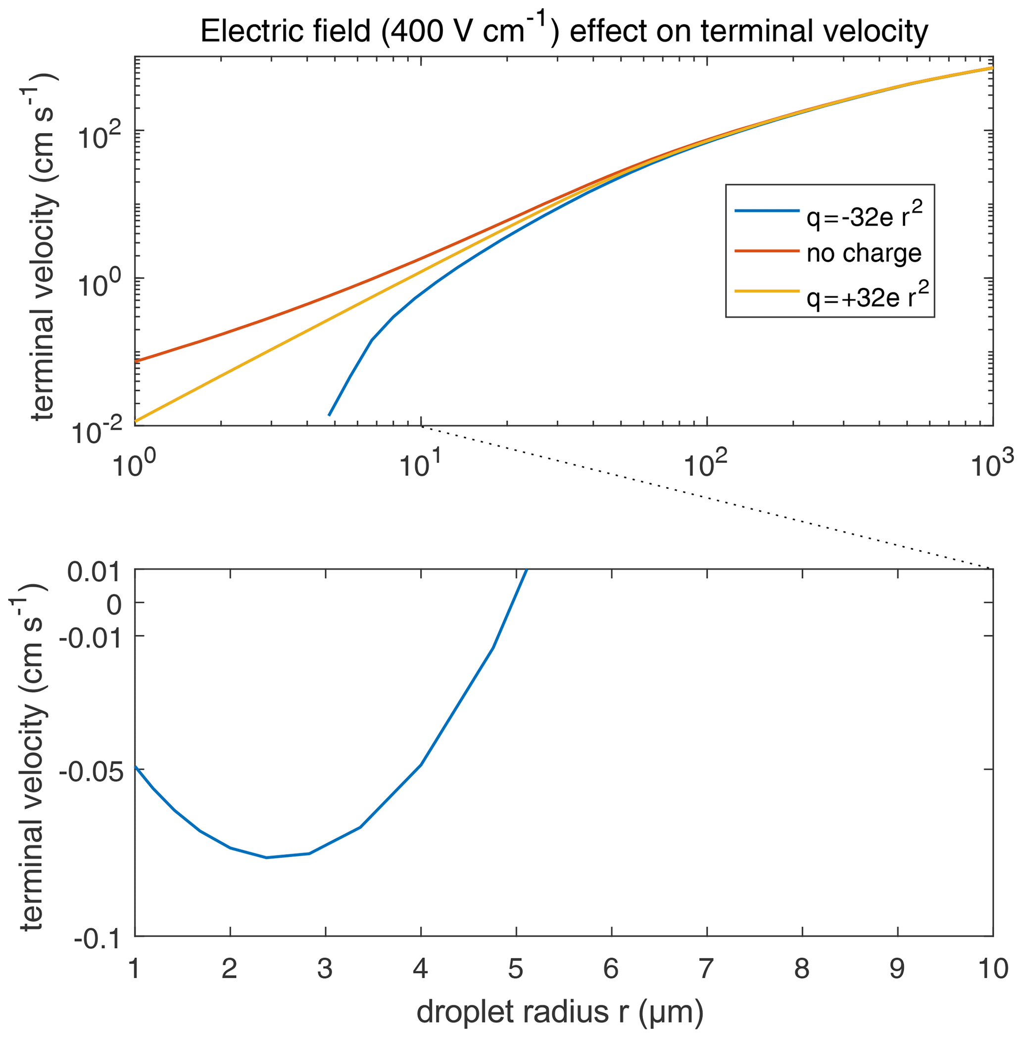
Figure 16Terminal velocities of droplets in an external electric field 400 V cm−1. Different lines denote different droplet charge conditions. It is significant that the terminal velocity of negatively charged droplets smaller than 5 µm turn upwards, leading to the discontinuity of the lower curve in the figure.
This study still neglects some possible electrostatic effects in the collision–coalescence process. The electrostatic effect on coalescence efficiency ε is neglected. Rebound (collision but not coalescence) happens because of an air film temporarily trapped between the two surfaces, which is a barrier to coalescence. This barrier may be overcome by a strong electric attraction occurring at a small distance. Many experiments show that electric charges and fields would enhance coalescence efficiency, such as those by Jayaratne and Mason (1964) and Beard et al. (2002). The latter experiment indicates that even a minimal electric charge incapable of enhancing collision can significantly increase ε, while the marginal utility of larger electric charges on ε is very small. However, there is no proper numerical model to evaluate the effect. Therefore, this study may underestimate the electrostatic effect on the droplet collision–coalescence process.
Induced charge redistribution is also neglected when rebound happens. For instance, let us consider a rebound event in a positive (downward) electric field. The larger droplet is often above the smaller droplet, and the smaller one will carry positive charge instantaneously, according to electrostatic induction, then move apart. The rebound would cause a charge redistribution between the pair. This may lead to some change in the evolution of clouds.
The effect of electric charges and atmospheric electric fields on cloud droplet collision–coalescence and on the evolution of cloud droplet size distribution is studied numerically. The equations of motion for cloud droplets are solved to obtain the trajectories of droplet pair of any radii (2 to 1024 µm) and charges (−32 to +32 r2, in units of elementary charge; droplet radius r, in units of µm) in different strengths of downward electric fields (0, 200, and 400 V cm−1). Based on trajectories, we determine whether a droplet pair collide or not. Thus, collision efficiencies for the droplet pairs are derived. It is seen that the collision efficiency is increased by electric charges and fields, especially when the droplet pair are oppositely charged or both negatively charged in a downward electric field. We consider these effects as being the electrostatic effects. The increase in collision efficiency is particularly significant for a pair of small droplets.
With the collision efficiencies derived in this study, the SCE is solved to simulate the evolution of cloud droplet size distribution under the influence of electrostatic effects. The initial droplet size distributions include , 9, and 6.5 µm, and the initial electric conditions include uncharged and charged droplets (with a charge amount proportional to droplet surface area) in different strengths of electric fields (0, 200, and 400 V cm−1). The magnitudes of electric charges and fields used in this study represent the observed atmospheric conditions. In the natural precipitation process, the charge amount, the strength of electric fields, and the timescale of the evolution are similar to those in this study. It is seen that the electrostatic effects are not notable for clouds with initial µm, since the initial radius is large enough to start a gravitational collision quickly. For clouds with initial µm, electric charges could evidently enhance droplet collision compared to the uncharged condition when there is no electric field, and the existence of electric fields further accelerates the collision–coalescence and the formation of large drops. For clouds with initial µm, it is difficult for gravitational collision to occur. The enhancement of droplet collision merely by an electric charge without a field is still not significant, but electric fields could remarkably enhance the collision process. These results indicate that clouds with droplet sizes smaller than 10 µm are more sensitive to electrostatic effects, which can significantly enhance the collision–coalescence process and trigger the raindrop formation.
It is known that the increase in aerosol number and, therefore, the decrease in cloud droplet size lead to suppressed precipitation and a longer cloud lifetime. But, with the electrostatic effect, the aerosol effect can be mitigated to a certain extent. The three initial droplet size distributions used in this study, with , 9, and 6.5 µm, have an initial droplet number concentration of 71, 325, and 851 cm−3, respectively. The three cases can represent different aerosol conditions. Smaller droplets size and higher droplet number concentration represent a more polluted condition. It is seen that the collision–coalescence process is significantly slowed down as changes from 15 to 9 µm, and to 6.5 µm. It takes about 30, 60, and 120 min, respectively, for the three cases to form a mode of 200 µm in the droplet size distribution. We consider this as being an aerosol effect. When the electrostatic effect is considered, the case with µm now only takes about 45 min to form the mode of 200 µm. Therefore, the enhancement of raindrop formation due to electrostatic effects can mitigate the suppression of rain due to aerosols.
Data and programs are available from Shian Guo (guoshian@pku.edu.cn) upon request.
SG developed the model, wrote the codes of the program, and performed the simulation. HX advised on the case settings of the numerical simulation. HX and SG worked together to prepare the paper.
The authors declare that they have no conflict of interest.
We are grateful to Jost Heintzenberg and Shizuo Fu for their constructive discussions on this study.
This study has been supported by the National Innovation and Entrepreneurship Training Program for College Students and the Chinese Natural Science Foundation (grant no. 41675134).
This paper was edited by Patrick Chuang and reviewed by three anonymous referees.
Albrecht, B. A.: Aerosols, cloud microphysics, and fractional cloudiness, Science, 245, 1227–1230, https://doi.org/10.1126/science.245.4923.1227, 1989.
Baumgaertner, A. J. G., Lucas, G. M., Thayer, J. P., and Mallios, S. A.: On the role of clouds in the fair weather part of the global electric circuit, Atmos. Chem. Phys., 14, 8599–8610, https://doi.org/10.5194/acp-14-8599-2014, 2014.
Beard, K. V.: Terminal velocity and shape of cloud and precipitation drops aloft, J. Atmos. Sci., 33, 851–864, https://doi.org/10.1175/1520-0469(1976)033<0851:TVASOC>2.0.CO;2, 1976.
Beard, K. V. and Ochs III, H. T.: Collection and coalescence efficiencies for accretion, J. Geophys. Res., 41, 863–867, https://doi.org/10.1029/JD089iD05p07165, 1984.
Beard, K. V., Durkee, R. I., and Ochs, H. T.: Coalescence efficiency measurements for minimally charged cloud drops, J. Atmos. Sci., 59, 233–243, https://doi.org/10.1175/1520-0469(2002)059<0233:CEMFMC>2.0.CO;2, 2002.
Bott, A.: A flux method for the numerical solution of the stochastic collection equation, J. Atmos. Sci., 55, 2284–2293, https://doi.org/10.1175/1520-0469(1998)055<2284:AFMFTN>2.0.CO;2, 1998.
Davis, M. H.: Two charged spherical conductors in a uniform electric field: Forces and field strength, Q. J. Mech. Appl. Math., 17, 499–511, https://doi.org/10.1093/qjmam/17.4.499, 1964.
Eow, J. S., Ghadiri, M., Sharif, A. O., and Williams, T. J.: Electrostatic enhancement of coalescence of water droplets in oil: a review of the current understanding, Chem. Eng. J., 84, 173–192, https://doi.org/10.1016/S1385-8947(00)00386-7, 2001.
Hamielec, A. E. and Johnson, A. I.: Viscous flow around fluid spheres at intermediate Reynolds numbers, Can. J. Chem. Eng., 40, 41–45, https://doi.org/10.1002/cjce.5450400202, 1962.
Hamielec, A. E. and Johnson, A. I.: Viscous flow around fluid spheres at intermediate Reynolds numbers (II), Can. J. Chem. Eng., 41, 246–251, https://doi.org/10.1002/cjce.5450410604, 1963.
Harrison, R. G. and Carslaw, K. S.: Ion-Aerosol-Cloud Processes in the Lower Atmosphere, Rev. Geophys., 41, 1012, https://doi.org/10.1029/2002RG000114, 2003.
Harrison, R. G., Nicoll, K. A., and Ambaum, M. H. P.: On the microphysical effects of observed cloud edge charging, Q. J. Roy. Meteor. Soc., 141, 2690–2699, https://doi.org/10.1002/qj.2554, 2015.
Jayaratne, O. W. and Mason, B. J.: The coalescence and bouncing of water drops at an air/water interface, P. R. Soc. London, 280, 545–565, https://doi.org/10.1098/rspa.1964.0161, 1964.
Khain, A., Arkhipov, V., Pinsky, M., Feldman, Y., and Ryabov, Y.: Rain enhancement and fog elimination by seeding with charged droplets. Part I: theory and numerical simulations, J. Appl. Meteorol., 43, 1513–1529, https://doi.org/10.1175/JAM2131.1, 2004.
Klimin, N. N., Rivkind, V. Y., and Pachin, V. A.: Collision efficiency calculation model as a software tool for microphysics of electrified clouds, Meteorol. Atmos. Phys., 53, 111–120, https://doi.org/10.1007/BF01031908, 1994.
Lamb, D. and Verlinde, J.: Physics and Chemistry of Clouds, Cambridge University Press, New York, USA, 2011.
Miles, N. L., Verlinde, J., and Clothiaux, E. E.: 2000 Cloud droplet size distributions in low-level stratiform clouds, J. Atmos. Sci., 57, 295–311, https://doi.org/10.1175/1520-0469(2000)057<0295:CDSDIL>2.0.CO;2, 2000.
Pinsky, M. and Khain, A.: Collision efficiency of drops in a wide range of Reynolds numbers: effects of pressure on spectrum evolution, J. Atmos. Sci., 58, 742–763, https://doi.org/10.1175/1520-0469(2001)058<0742:CEODIA>2.0.CO;2, 2000.
Pruppacher, H. R. and Klett, J. D.: Microphysics of Clouds and Precipitation, Kluwer Academic Publishers, Dordrecht, the Netherlands, 1997.
Schlamp, R. J., Grover, S. N., Pruppacher, H. R., and Hamielec, A. E.: A numerical investigation of the effect of electric charges and vertical external electric fields on the collision efficiency of cloud drops, J. Atmos. Sci., 33, 1747–1755, https://doi.org/10.1175/1520-0469(1976)033<1747:ANIOTE>2.0.CO;2, 1976.
Takahashi, T.: Measurement of electric charge of cloud droplets, drizzle, and raindrops, Rev. Geophys. Space. Ge., 11, 903–924, https://doi.org/10.1029/RG011i004p00903, 1973.
Telford, J. W.: A new aspect of coalescence theory, J. Meteorol., 12, 436–444, 1955.
Tinsley, B. A., Zhou, L., and Plemmons, A.: Changes in scavenging of particles by droplets due to weak electrification in clouds, Atmos. Res., 79, 266–295, https://doi.org/10.1016/j.atmosres.2005.06.004, 2006.
Twomey, S.: Pollution and the planetary albedo, Atmos. Environ., 8, 1251–1256, https://doi.org/10.1016/0004-6981(74)90004-3, 1974.
Wallace, J. M. and Hobbs, P. V.: Atmospheric Science: An Introductory Survey, Second Edition, Academic Press, Elsevier Academic Press, Boston, USA, 2006.
Wang, L. P., Ayala, O., and Grabowski, W. W.: Improved Formulations of the Superposition Method, J. Atmos. Sci, 62, 1255–1266, https://doi.org/10.1175/JAS3397.1, 2005.
Warner, J.: The water content of cumuliform cloud, Tellus, 7, 449–457, https://doi.org/10.3402/tellusa.v7i4.8917, 1955.
Zhou, L., Tinsley, B. A., and Plemmons, A.: Scavenging in weakly electrified saturated and subsaturated clouds, treating aerosol particles and droplets as conducting spheres, J. Geophys. Res., 114, D18201, https://doi.org/10.1029/2008JD011527, 2009.
- Abstract
- Introduction
- Stochastic collection equation
- Method for calculating terminal velocity and collision efficiency with electrostatic effects
- Model setup for solving the stochastic collection equation
- Results
- Discussion
- Conclusion
- Code and data availability
- Author contributions
- Competing interests
- Acknowledgements
- Financial support
- Review statement
- References