Using TROPOspheric Monitoring Instrument (TROPOMI) measurements and Weather Research and Forecasting (WRF) CO modelling to understand the contribution of meteorology and emissions to an extreme air pollution event in India

Several ambient air quality records corroborate the severe and persistent degradation of air quality over northern India during the winter months, with evidence of a continued, increasing trend of pollution across the Indo-Gangetic Plain (IGP) over the past decade. A combination of atmospheric dynamics and uncertain emissions, including the post-monsoon agricultural stubble burning, make it challenging to resolve the role of each individual factor. Here we demonstrate the potential use of an atmospheric transport model, the Weather Research and Forecasting model coupled with chemistry (WRF–Chem) to identify and quantify the role of transport mechanisms and emissions on the occurrence of the pollution events. The investigation is based on the use of carbon monoxide (CO) observations from the TROPOspheric Monitoring Instrument (TROPOMI) on board the Sentinel-5 Precursor satellite and the surface measurement network, as well as the WRF–Chem simulations, to investigate the factors contributing to CO enhancement over India during November 2018. We show that the simulated column-averaged dry air mole fraction (XCO) is largely consistent with TROPOMI observations, with a spatial correlation coefficient of 0.87. The surface-level CO concentrations show larger sensitivities to boundary layer dynamics, wind speed, and diverging source regions, leading to a complex concentration pattern and reducing the observation-model agreement with a correlation coefficient ranging from 0.41 to 0.60 for measurement locations across the IGP. We find that daily satellite observations can provide a first-order inference of the CO transport pathways during the enhanced burning period, and this transport pattern is reproduced well in the model. By using the observations and employing the model at a comparable resolution, we confirm the significant role of atmospheric dynamics and residential, industrial, and commercial emissions in the production of the exorbitant level of air pollutants in northern India. We find that biomass burning plays only a minimal role in both column and surface enhancements of CO, except for the state of Punjab during the high pollution episodes. While the model reproduces observations reasonably well, a better understanding of the factors controlling the model uncertainties is essential for relating the observed concentrations to the underlying emissions. Overall, our study emphasizes the importance of undertaking rigorous policy measures, mainly focusing on reducing residential, commercial, and industrial emissions in addition to actions already underway in the agricultural sectors.

1 Introduction

Biomass burning (BB) has been recognized as the second-largest source of radiatively and chemically active trace gases (e.g. carbon monoxide – CO; carbon dioxide – CO₂; and sulfur dioxide – SO₂) and aerosols (e.g. particulate matter – PM₁₀ and PM_2.5) in the global atmosphere, which has significant implications for climatic change and human health (Andreae, 2001; Bond, 2004; Crutzen and Andreae, 1990; Guenther et al., 2006; Kaiser et al., 2012; van der Werf et al., 2017). According to previous reports, BB alone accounts for 59 % of black carbon (BC) emissions, one-third to one-half of global carbon monoxide (CO), and 20 % of nitrogen oxide (NO_x) emissions (Akagi et al., 2011; Andreae, 2019). Based on the model estimates of Ward et al. (2012), in the absence of fire-related emissions, there would be a reduction of about 40 ppm (parts per million) CO₂ from the current atmospheric concentration level, indicating the importance of fire activities for the global carbon budget.

In India, emissions from open biomass burning include significant contributions from agricultural crop residue burning, in addition to forest and grassland fires, and play an essential role in terms of releasing total carbon content to the atmosphere. Agricultural stubble burning during the post-harvesting period is one of the main kinds of biomass burning practices used in India to clear the land to make it suitable for the next crop (Tai-Yi, 2012; Zha et al., 2013). According to previous estimates, crop waste open burning, which includes its use in residential heating and cooking, is responsible for 78 %–83 % (116–289 Tg yr⁻¹) of the total biomass burned in India during the year 2001, while rest of the contributions are from forest fires (Venkataraman et al., 2006). As per the previous studies, the primary crop residues generated in India are rice straw (112 Mt), wheat straw (109.9 Mt), rice husk (22.4 Mt), sugarcane tops (97.8 Mt), and bagasse (101.3 Mt), the major part of which is burnt in the open air (Lasko and Vadrevu, 2018). Most of these burning activities are found over the northern part of India along the foothills of the Himalayas known as the Indo-Gangetic Plains (hereafter called the IGP). The IGP is a highly populated and very important agro-eco region in South Asia, which includes the states of Punjab, Haryana, Bihar, Uttar Pradesh, and West Bengal. The region occupies nearly 20 % of the total geographical area of India and contributes about 42 % to India's total grain production (Tripathi et al., 2007). Based on VIIRS (Visible Infrared Imaging Radiometer Suite) thermal anomalies, a recent study has estimated burnt crop residues of 20.4 Mt and 9.6 Mt in Punjab and Haryana for the agricultural year 2017–2018 in which most of the residue burnt (>90 %) at the field was from rice and wheat crops (Singh et al., 2020).

Episodes of pollution events are a major concern in the IGP region, which worsen during post-monsoon and winter seasons (Cusworth et al., 2018; Dekker et al., 2019; Girach and Nair, 2014). According to the World Air Quality Report 2019 based on ambient PM_2.5 concentration, 14 of the top 20 most polluted cities in the world are located in the IGP region, which also includes India's capital region, Delhi. Earlier studies and reports attributed this to several reasons but mainly to crop residue burning over Punjab and Haryana, the two adjoining states of India's capital city of Delhi (Girach and Nair, 2014; Gupta et al., 2004; Sidhu et al., 1998). However, the contributions from different source sectors and source regions on Delhi's pollution levels still remain highly uncertain, which hinders the implementation of definitive measures to address pollution events. A recent study reported a general lack of reliable data and research efforts on biomass-burning-related issues on environment and human health (Yadav et al., 2017). Since agricultural stubble burning is a practice prohibited by law in India, official surveys conducted to estimate the extent of fire emission are not reliable. There is, therefore, a critical need to improve the current knowledge base to help to make future policies and implement mitigation strategies.

Kaiser et al. (2012) demonstrated an approach for the calculation of biomass burning emissions by assimilating satellite-based fire radiative power (FRP) observations. Along with FRP data, this approach derives the combustion rate and trace gas emissions subsequently, with land-cover-specific conversion factors and emission factors compiled through literature surveys. While the FRP-based approach has a clear advantage of enhancing accuracy compared to other inventory-based data sets, such as the Global Fire Emission Database (GFED), several studies have indicated inaccuracies in the FRP-derived biomass burning products due to instrument limitations and usage of conversion factors (Cusworth et al., 2018; Dekker et al., 2019; Huijnen et al., 2016; Kaiser et al., 2012; Mota and Wooster, 2018). The recent availability of greenhouse gas satellite observations with unprecedented data density at high spatial and temporal resolution paves the more direct way for a detailed study on the origin, distribution, and extent of trace gas levels over a vast domain on a monthly to daily basis. Carbon monoxide (CO) is one of the major gases emitted from biomass burning and incomplete fossil fuel combustion. The major sink of CO is its reaction with the hydroxyl radical (OH) to form CO₂ and precursor tropospheric ozone. The lifetime of CO in the atmosphere is between several weeks and several months and varies with the location and season, depending on the oxidizing capacity of the environment (Jaffe, 1968). Compared to CO₂ and methane (CH₄), the short lifetime of CO makes it easier to detect from the background concentration level, and thus, it can be a good tracer of pollution transport (Dekker et al., 2017). Therefore, CO can be used as a proxy for the anthropogenic emissions of other pollutants, for example, emissions of important greenhouse gases (GHGs) such as CO₂ (Gamnitzer et al., 2006).

The TROPOspheric Monitoring Instrument (TROPOMI), on board the Sentinel-5 Precursor satellite, has been measuring various trace gases, including CO, since November 2017 (Landgraf et al., 2016; Borsdorff, 2018; Borsdorff et al., 2018; Schneising et al., 2019, 2020a). TROPOMI measures with a high spatial (7 km × 7 km) and temporal resolution (global daily coverage, not accounting for cloud and aerosol contamination). The unprecedented data density, with a high spatial and temporal resolution, makes TROPOMI useful for obtaining information from the city scale to regional scale. The validation of the TROPOMI retrieval with ground-level measurements and model simulations has confirmed the high quality of the measurements, with a high signal-to-noise ratio, indicating the usefulness of the data collected (Borsdorff, 2018; Borsdorff et al., 2018; Schneising et al., 2019, 2020a).

In this study, we make use of CO observations from TROPOMI (see Sect. 2.1) and the surface measurement network to investigate different regional sources of CO in terms of their contribution to the total column and surface-level concentrations during high pollution episodes in the winter season.  By comparing CO measurements with high-resolution model simulations generated by WRF–Chem-GHG, we aim to understand the contribution of different sources to the observed CO enhancement. In particular, we focus on CO enhancement caused by the emissions from both biomass burning and anthropogenic activities and their relative roles in the severe air pollution of major cities nearby. This paper aims to address the following questions: (1) how large is the CO enhancement over northern India detected by TROPOMI during the agricultural stubble burning period? (2) What is the regional contribution of CO emissions over India during the entire year of 2018? (3) How good is the agreement between the WRF–Chem-GHG and the observations, both at ground level and integrated across the column? (4) How does the column respond to the spatio-temporal variations in surface emissions, particularly biomass emissions? (5) What is the role of different emission sources in terms of their contribution to the enhanced concentration level during the high pollution episodes over India? An analysis focusing on identifying the sources contributing to the high pollution event in northern India during November 2017, using WRF modelling and TROPOMI preliminary operational data was reported in Dekker et al. (2019). Here, we present the analysis for the succeeding year, i.e. November 2018. Additionally, this study differs from the previous study as follows. The present study (1) uses the retrievals from both algorithms of the Weighting Function Modified Differential Optical Absorption Spectroscopy (TROPOMI/WFM-DOAS; Schneising et al., 2019; see Sect. 2.1) and TROPOMI Shortwave Infrared Carbon Monoxide Retrieval (TROPOMI/SICOR; Landgraf et al., 2016); (2) examines the regional distribution of CO for the entire year, (3) employs different model configuration such as the model domain size, vertical eta levels, and planetary boundary layer scheme; (4) prescribes a different anthropogenic emission inventory that also includes hourly variations; and (5) utilizes the entire month, which includes biomass burning and non-biomass burning periods to obtain a more detailed view of the dispersion to nearby places.

2 Data

2.1 TROPOMI column observations

The TROPOMI onboard the Sentinel-5 Precursor satellite (S5P), has been measuring various trace gases, including CO, since November 2017 (Landgraf et al., 2016; Borsdorff, 2018; Borsdorff et al., 2018; Schneising et al., 2019, 2020a). The TROPOMI instrument consists of a shortwave infrared (SWIR), nadir-viewing imaging spectrometer, which measures radiances around 2.3 µm wavelength, from which the total column mixing ratio (XCO) is retrieved (Schneising et al., 2019; Landgraf et al., 2016). Due to the wide swath of about 2600 km, the instrument is able to cover the whole globe on a daily basis, capturing full scenes of continuous observations in cloud-free conditions (Schneising et al., 2019, 2020a). As a result of the observation of reflected solar radiation in the SWIR part of the solar spectrum, TROPOMI yields atmospheric carbon monoxide measurements with high sensitivity to all altitude levels, including the planetary boundary layer, and is thus well suited for studying emissions from fires (Schneising et al., 2020a).

For this study, we use TROPOMI CO data for November 2018, retrieved using the scientific algorithm TROPOMI/WFM-DOAS, optimized to retrieve vertical columns of carbon monoxide and methane simultaneously (Schneising et al., 2019). Additionally, we use TROPOMI operational CO data (TROPOMI/SICOR CO; Borsdorff, 2018; Borsdorff et al., 2018) to examine the consistency of these two observational products over India. The TROPOMI/SICOR and TROPOMI/WFM-DOAS algorithms differ in many aspects, including radiative transfer models, inversion schemes and the quality filtering method used. Whereas TROPOMI/WFM-DOAS retrievals are limited to cloud-free scenes, TROPOMI/SICOR aims to retrieve CO columns for cloudy ground pixels too. A global comparison between these two data sets from December 2018 (Schneising et al., 2019) shows a very similar spatial CO pattern for both algorithms, with a high correlation coefficient of 0.98 and a regression factor close to the 1:1 line, confirming a good agreement between the two data sets. An overview of the TROPOMI data sets used in this study is provided in Table 1, and additional details are provided in the following two sub-sections.

Table 1 Overview of the TROPOMI CO products used in this study.

2.1.1 Scientific TROPOMI/WFMD CO product

The WFM-DOAS retrieval algorithm was initially developed for the SCanning Imaging Absorption spectroMeter for Atmospheric CartograpHY (SCIAMACHY) instrument on board the ENVISAT satellite (Buchwitz et al., 2006, 2007; Schneising et al., 2011, 2014) and has recently been adjusted for XCO retrieval from TROPOMI (Schneising et al., 2019, 2020a). TROPOMI/WFM-DOAS uses a least squares approach, which retrieves XCO from the shortwave infrared spectra recorded by the TROPOMI instrument. The TROPOMI/WFM-DOAS CO retrievals (hereafter referred to as TROPOMI/WFMD) have undergone direct validation with independent reference data from the worldwide total carbon column observing network (TCCON; Wunch et al., 2011), which consists of ground-based Fourier transform spectrometer (FTS) instruments with a well-controlled light path. TCCON measurements are calibrated to the World Meteorological Organization (WMO) scale. As per this validation, TROPOMI/WFMD XCO has a systematic error of 1.9 ppb (parts per billion) and a random error of 5.1 ppb (Schneising et al., 2019).

2.1.2 Operational TROPOMI/SICOR CO product

The Shortwave Infrared Carbon Monoxide Retrieval (SICOR) algorithm is used to retrieve the operational CO product (hereafter referred to as TROPOMI/SICOR; Landgraf et al., 2016; Borsdorff, 2018; Borsdorff et al., 2018). The validation study of TROPOMI/SICOR with the CAMS data shows a good agreement with global mean difference of +3.2 % and a Pearson correlation coefficient of 0.97 (Borsdorff et al., 2018). For the Indian region, a 2.9 % difference was found with CAMS, with a standard deviation of 6 % and a Pearson correlation coefficient of 0.9 (Borsdorff, 2018). As per the validation of TROPOMI/SICOR with ground-based total column measurements of TCCON, a mean bias of 6 ppb with a standard deviation of 3.9 and 2.4 ppb has been found for clear and cloudy skies, respectively (Borsdorff, 2018).

2.2 Ground-level observations

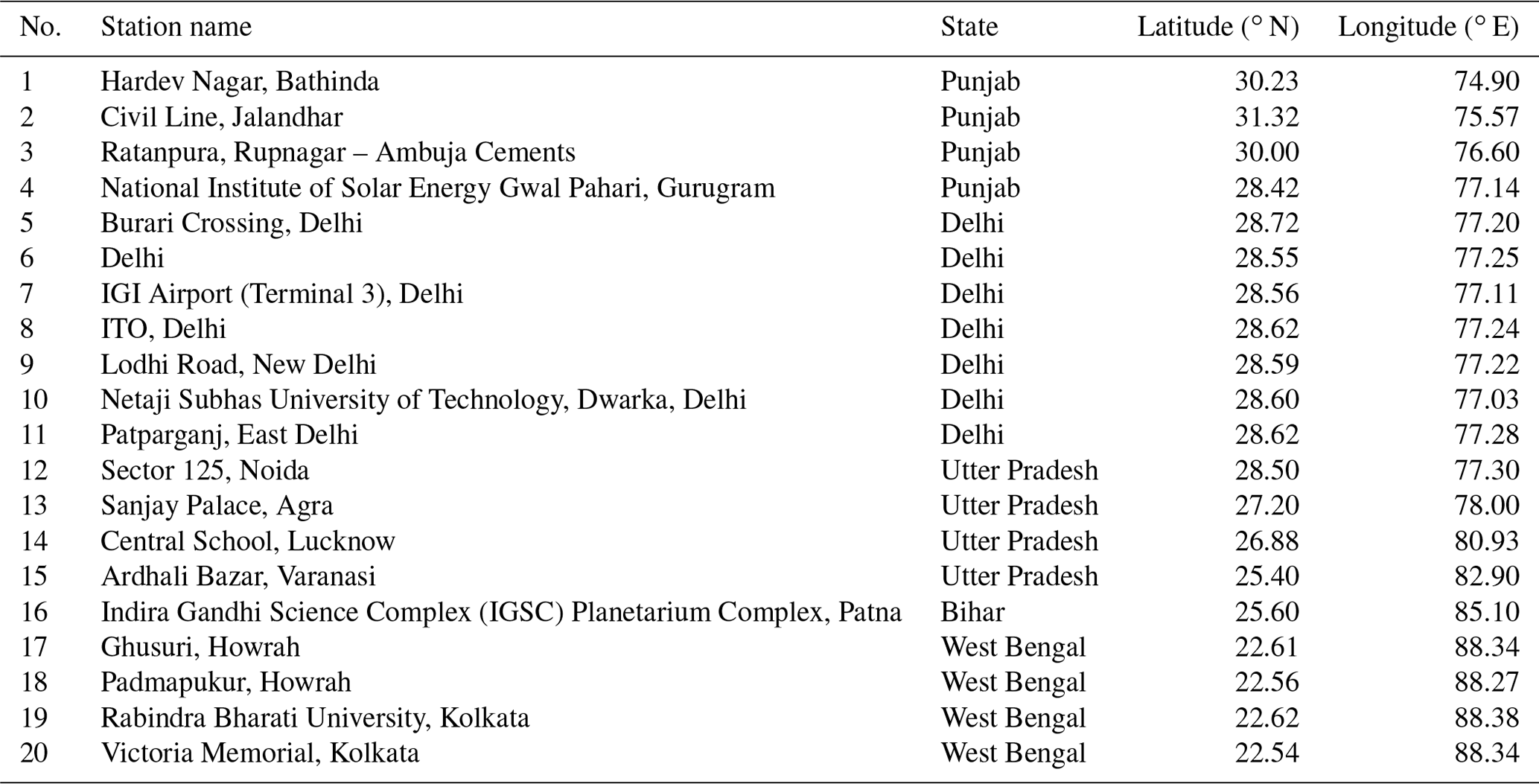
To assess the model performance against the surface-level measurements, we use measurements from ground-based air quality monitoring network maintained by the Central Pollution Control Board (CPCB) of India. The measurements of CO are performed using CO analysers based on non-dispersive infrared spectroscopy, and the data are provided as 6 h averages via a publicly accessible online portal (https://app.cpcbccr.com/ccr/#/caaqm-dashboard-all/caaqm-landing/data, last access: 16 March 2020). Though we have analysed CO measurements available from all stations for the period of 3–20 November 2018, measurement stations that are too close to local emissions sources or show extremely large and ambiguous variations in which the stability of the analyser could be questioned were excluded for the evaluation. All the stations used for this evaluation are listed in Table 2.

Table 2 List of ground-level measurement stations used for this study.

3 WRF–Chem-GHG model

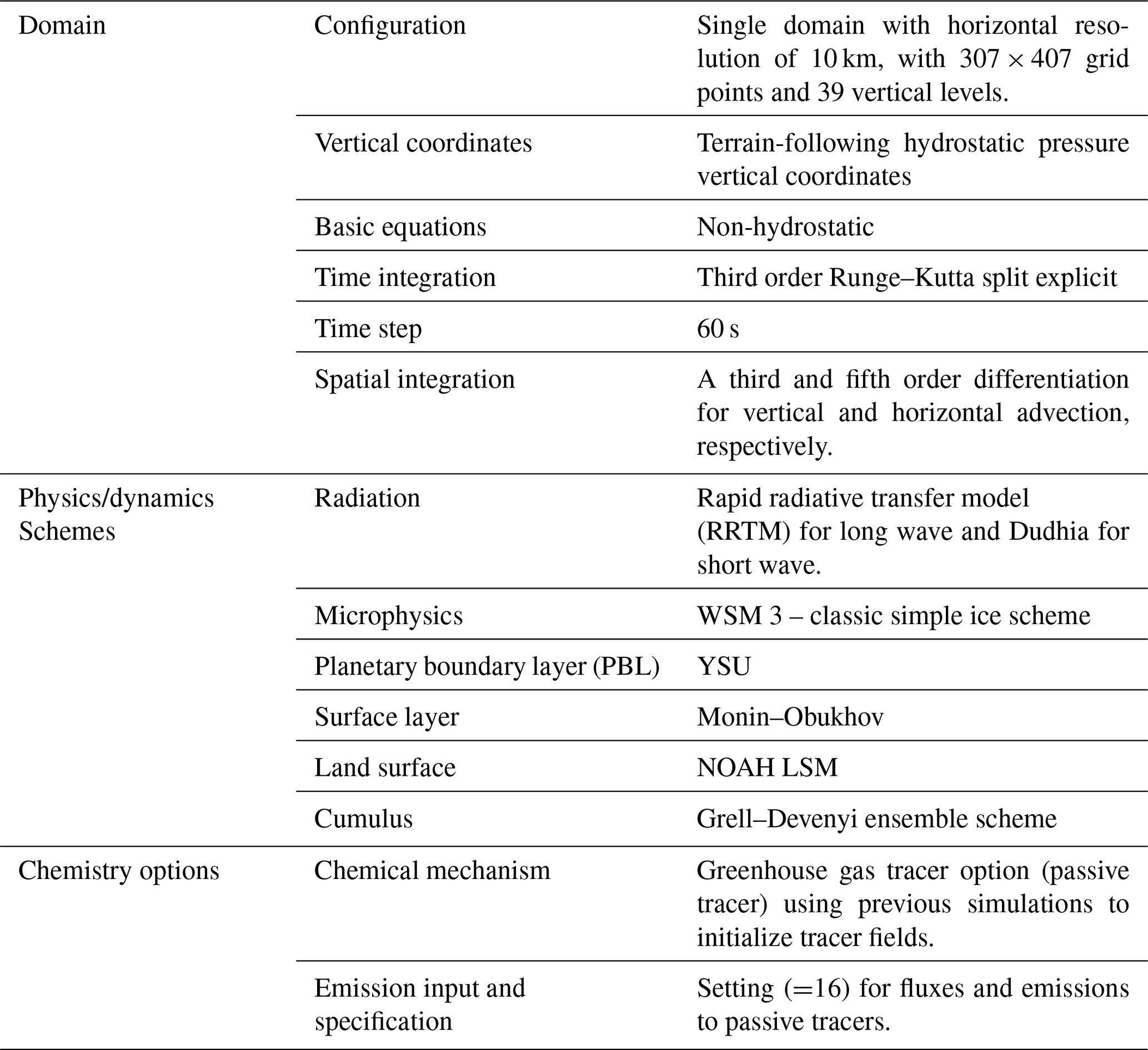
We utilize a high-resolution modelling framework based on a WRF–Chem-GHG (version 3.9.1.1; hereafter referred to as WRF) to simulate CO concentrations at a spatial resolution of 10 km × 10 km) and a temporal resolution of 1 h. The model solves the compressible Euler non-hydrostatic equations and uses a terrain-following hydrostatic pressure coordinate system in the vertical direction (Skamarock et al., 2008). In our case, simulations have 39 vertical levels extending from the surface to 50 hPa (∼ 20 km), and the model domain describes a region with a spatial extent of 3500 km × 2500 km, covering the Indian domain and some parts of Bangladesh, China, Nepal, and Pakistan.

For meteorological initial and boundary conditions, we have taken fifth generation ECMWF reanalysis (ERA5) data, on an hourly basis, with a horizontal resolution of 0.25^∘ × 0.25^∘. The model is re-initialized each day with ERA5 meteorology and allowed a 6 h spin-up time. For CO concentration fields, initial and boundary conditions are prescribed from the Copernicus Atmosphere Monitoring Service (CAMS re-analysis data). CAMS provides the estimated mixing ratios of CO, with a spatial resolution of 0.25^∘ × 0.25^∘ at a temporal resolution of 6 h on 60 vertical levels. For CO simulations, we have mainly used anthropogenic and biomass burning emissions tracers from external data sets. To represent anthropogenic contributions, we use the global EDGAR emission inventory (Emission Database for Global Atmospheric Research; version 4.3.2; the year 2012) data at a spatial resolution of 0.1^∘ × 0.1^∘. EDGAR provides global inventories for GHG emissions and air pollutants on an annual basis, but we apply time factors in order to create hourly emissions. The time factors are based on the step function time profiles, based on the TROTREP/POET profiles provided in Olivier et al., 2003. We use the CO emission data from the Global Fire Assimilation System (GFAS) for the year of 2018 to represent biomass burning emissions. GFAS is a satellite-based fire emission inventory (http://apps.ecmwf.int/datasets/data/cams-gfas/, last access: 10 March 2019), which provides biomass burning emissions daily at a global horizontal resolution of 0.1^∘ × 0.1^∘. The inventory calculates the fire emissions by assimilating FRP observations from MODIS instruments on the polar-orbiting satellites, Aqua and Terra, which observe the thermal radiation from fire activities at wavelengths around 3.9 and 11 µm (Kaiser et al., 2012). It achieves higher spatial and temporal (daily) resolution than almost any other inventory and can estimate near-real-time emissions. A number of studies have reported the underestimation of GFAS in fire emissions due to the limitations of the MODIS instruments, which do not capture all active fires such as small fires (Cusworth et al., 2018; Dekker et al., 2019; Huijnen et al., 2016; Kaiser et al., 2012; Mota and Wooster, 2018; Pan et al., 2020).

All these emissions fluxes are gridded to WRF's Lambert conformal conic projection grid, with 10 km horizontal resolution, conserving the total mass of emissions. These fluxes are added to the first model layer and transported separately as tagged tracers (Pillai et al., 2016). In order to account for the CO transported from the boundaries, we used CAMS CO data derived at the boundary conditions and refer to this CO tracer as background, meaning the concentration without considering any sources or sinks in the targeted domain. The total CO is then calculated as CO total equals CO background (BCK) plus CO anthropogenic (ANT) plus CO biomass (BBU).

Utilizing the emission tracers mentioned above and the multiple physics and chemistry options and dynamics schemes (see Table 3), model simulations of CO are performed for the period 1–30 November 2018. To assess the impact of small fires on our atmospheric CO mixing ratio simulations, we use another satellite-based fire inventory, the Global Fire Emissions Database version 4s (GFED4s), which includes small fires (Randerson et al., 2012; van der Werf et al., 2017). The dry matter (DM) emissions from GFED4s are converted to CO emissions, using emissions factors given in Akagi et al. (2011).

Table 3 Overview of WRF–Chem model set-up.

The model setup does not include the deposition and chemical formation of CO from volatile organic compounds (VOCs). Compared to the direct CO sources, such as anthropogenic and biomass burning emissions over the model domain, the indirect source from VOC oxidation is much smaller, and the deposition processes are minor compared to the transport of CO out of the model domain (Dekker et al., 2017). Also, the oxidation with the hydroxyl (OH) radical is not considered. Based on a few sensitivity simulations, Dekker et al. (2017) reported a slight (4 %) net decrease in enhancement when including chemical reactions of CO and concluded that the CO enhancement pattern is hardly affected by VOCs and OH oxidation.

4 Methods

4.1 Comparison of WRF simulations with satellite column observations

To evaluate the performance of WRF, we have performed a comparison study on a daily and monthly basis using TROPOMI/WFMD column CO (XCO) data during the period 1–30 November 2018 over the Indian domain. The TROPOMI/WFMD data set also provides the column averaging kernel vector (AK) describing the vertical sensitivity of the retrieved CO column to the partial column at different vertical levels (Schneising et al., 2019). In order to compare the satellite data with model simulations quantitatively, we have to use the AK to take into account the vertical sensitivity of the instrument. In the data set, the elements of the AK mostly have values close to 1, meaning that the instrument is sensitive to the full column of CO. As such, the prior estimates have a negligible contribution to the retrieved columns. To compare the simulated concentration fields with the satellite observations, the simulated pressure-weighted column-averaged dry air mole fraction after applying the averaging kernel, c_avgk, is calculated as follows:

$$\begin{array}{}\text{(1)}& {\mathit{c}}_{\mathrm{avgk}}=c+{\displaystyle \frac{\mathrm{1}}{{\mathit{m}}_{\mathrm{0}}}}{\sum }_{l=\mathrm{1}}^n\left({\mathit{m}}_l\left(\mathrm{1}-{\mathit{A}}_l\right)({\mathit{x}}_T^l-x^l\right).\end{array}$$

In this equation, l is the index of the vertical layer, n is the number of vertical layers, and A_l the corresponding column-averaging kernel of the TROPOMI/WFMD algorithm. c is the pressure-weighted column averaged dry air mole fraction calculated from model simulations. x_T is the a priori dry air mole fraction profile used by the TROPOMI/WFMD retrieval algorithm, which is also provided in the data product, and x is the model simulation. m_l is the mass of dry air for the corresponding layer, and m₀ is the total mass of dry air. For the comparison, we used only WRF simulations that correspond to the satellite sampling time. For a fair comparison between the satellite observations and model simulations, the averaging kernel matrix and a priori profile for each retrieval have been applied to the corresponding model output as explained in Eq. (1). For the ease of the statistical analysis, the observations, though comparable to the model resolution, are gridded to the WRF spatial resolution of 10 km × 10 km. Both TROPOMI/WFMD and WRF averaged data for the month of November and the period of 6–9 November (enhanced biomass burning period as per the GFAS data) are utilized in this study to investigate the column enhancement by fire CO and their distribution over the study domain. During the enhanced biomass burning period, a definite enhancement in XCO is found over the biomass burning hotspot. The monthly averaged map shows decreased concentration levels over these hotspots, which is attributed to the CO concentration dispersion resulted by changing weather conditions.

4.2 Comparison of WRF simulations with ground-level observations

To evaluate the model performance at the surface level, we have performed a comparison study with the CO in situ measurements obtained from the ground-level pollution measurement stations. We use the data collected from 20 measurement stations within the IGP region, and evaluation is done against each station data. In order to see overall agreement for different regions in the IGP, we have averaged the data temporally using only the stations within the corresponding regions (Delhi, Punjab, and the IGP). The entire month is not used here due to the existence of data gaps from several stations. In order to avoid very localized influence and noise in the observed data, the 1 h data sets are temporally averaged to 6 h resolution.

5 Results and Discussions

5.1 Regional and seasonal variation of fire CO emission

In order to examine the spatio-temporal variations of the monthly fire CO emission, we have divided the entire region into five sub-regions, as shown in Fig. 1. The fire CO emissions show significant spatial and temporal variations, with predominant emissions over the Indo-Gangetic Plain (IGP), central India (CI), and northeastern India (NEI).

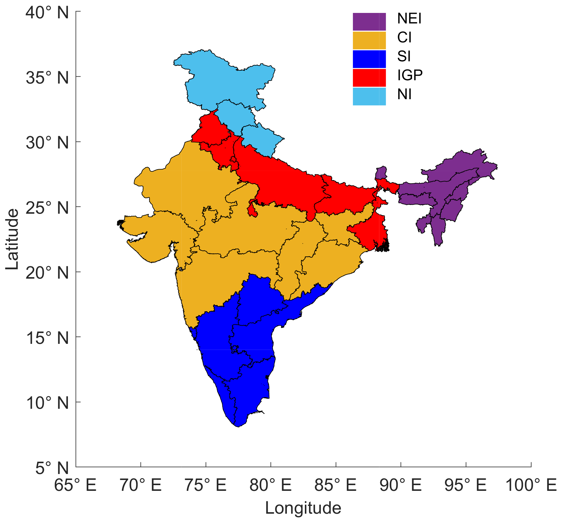
Figure 1 India is partitioned into the following five different areas for analysis: northeastern India (NEI), central India (CI), southern India (SI), the Indo-Gangetic Plain (IGP), and northern India (NI).

Figure 2 illustrates the integrated monthly fire CO emission for those regions in 2018. In most parts of India, the fire CO emissions peak during the March–April (pre-monsoon) period, accounting for about 76 % of the annual emissions. This is consistent with a study based on the fire counts analysis from 1998–2009, which reported that more than 75 % of the annual fires occurred during March–April (Sahu et al., 2015). Fire CO emissions during March are significantly higher when compared to other months, accounting for about 55 % of the annual emissions for India. Although having a small geographical area, the fire activities over northeastern India (NEI) made a significant contribution (57 %) to emissions during pre-monsoon months, while the IGP contributed only about 5 %. Central (CI) and southern regions (SI) of India add about 33 % towards the pre-monsoon fire CO emissions, while northern India (NI) shows fewer emissions during the whole year. However, emission spikes are seen in the IGP during the October–November (post-monsoon) period. This is also consistent with the distribution of total fire counts over IGP region during the post-monsoon period, as seen in Kulkarni et al. (2020). Over the IGP, the fire CO emissions show evident monthly variations, with a higher emission during the post-monsoon time compared to the pre-monsoon period. About 73 % of the country's total fire CO emissions during the post-monsoon period are from the IGP region. Of these IGP post-monsoon emissions, 70 % come from the northwestern states of the IGP (Punjab and Haryana). Over this region, 25 % of the total fire CO emissions happened within a short period during 6–9 November, which accounts for about 18 % of the country's post-monsoon total fire CO emissions. During the monsoon time, all regions are found to have fewer fire emissions, which can be attributed to the fact that rainfall leads to suppressed fire activity. In addition to the minimal possibility of fire activities during the rainy season, note that MODIS has only a limited capability to detect fire emissions over a cloudy scene. It should also be noted that very small fires involved can be missed due to MODIS instruments limitations, which may underestimate the fire CO emissions. With a finer spatial resolution of VIIRS (375 m) than MODIS (1 km), VIIRS detected ∼ 20 % more active fires at the spatial scale of 0.02^∘ × 0.02^∘ over Punjab and Haryana during the post-monsoon season (Liu et al., 2019).

Figure 2 (a) The monthly integrated GFAS fire CO emissions (mg/m² per month) over different regions of India (as seen in Fig. 1) during the year of 2018. (b) Integrated GFAS fire CO emission during 6–9 November 2018.

The observed monthly variations in fire emissions are mainly due to factors such as post-harvest crop residue burning, meteorological conditions (dry weather), and land-use practices (Habib et al., 2006). The fire activities during post- and pre-monsoon periods in India are mostly associated with the high level of crop residue burning during the post-harvest seasons (Sahu et al., 2015). Crop residue burning after harvesting is a general practice used by farmers to clear the land for the next crop. Over the IGP, there are mainly two seasonal crop seasons, known as kharif (primarily rice) and rabi (mainly wheat), which are harvested during post- and pre-monsoon seasons, respectively (Sahu et al., 2015). This results in temporal variations in residue burning emissions over the IGP. Compared to other parts of the IGP, the northwestern part of the IGP has the greatest preponderance of crop residues during the post-monsoon season (Singh and Panigrahy, 2011). Consistent with the spatial and seasonal differences in agricultural practices, we see a high level of fire CO emissions in this region during the short period of 6–9 November.

5.2 Enhanced XCO as observed by the satellite

Figure 3a shows the column CO dry mixing ratio retrieved from TROPOMI/WFMD over the Indian domain, averaged for the entire month of November and 6–9 November (most intense biomass burning period). During this period, higher values of column CO are observed over the northern part of India, particularly over the IGP region, compared to the other regions of India, showing higher values during the biomass burning period than the monthly average. A distinct enhancement in XCO can be observed during the biomass burning period, specifically over the states of Punjab and Haryana, with a distribution plume towards the southeasterly direction, including the regions of Delhi and Agra. Note that this emission hotspot is also seen in the GFAS inventory during the biomass burning period (Fig. 2). Consistency between the GFAS inventory and satellite observations suggests that the XCO enhancement over the northwestern part of the IGP during 6–9 November can be attributed to the crop residue burning that occurred over the Punjab region. The consistency check between two retrieval products (TROPOMI/WFMD and TROPOMI/SICOR) has resulted in a very similar spatial CO pattern for both algorithms, with a high correlation coefficient of 0.97, confirming the robustness of our findings between the two data sets over India (see Table 4). During early winter (November and December), the shallow planetary boundary layer (PBL) and low wind speed cause locally emitted gases to be trapped in the lower atmosphere, which is considered to be the primary cause for high concentrations during this period. For a better understanding of the role of transport and CO emissions from biomass burning to the distribution over the domain, we utilized WRF model simulations and performed a comparison study with the TROPOMI/WFMD observations, as explained in Sect. 4.1.

Table 4 Comparison between TROPOMI/WFMD and TROPOMI/SICOR products over India during the burning period and the full month of November 2018. Abbreviations N, MB, SD, and R correspond to the number of observations, mean bias, standard deviation of differences, and correlation coefficient, respectively.

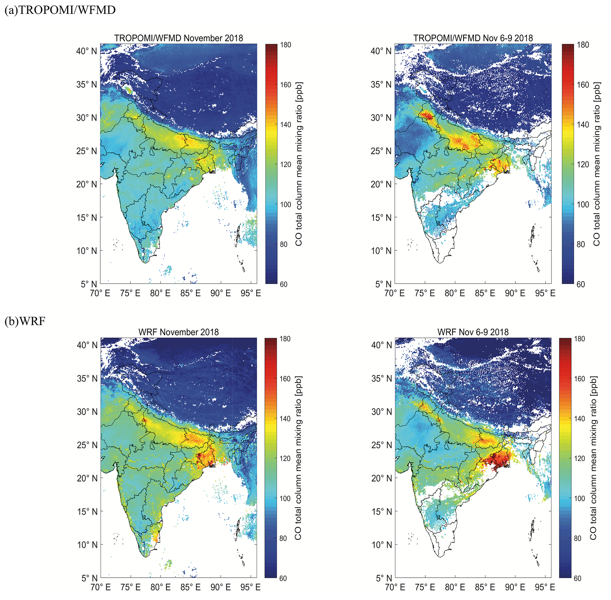
Figure 3 CO total column mixing ratios averaged for (a) TROPOMI/WFMD and (b) WRF over all of November 2018 (left panel) and from 6–9 November 2018 (right panel).

5.3 Validation of WRF

5.3.1 Agreement with column observations

We compared WRF simulations with TROPOMI/WFMD observations averaged over the days of peak burning and over the full month of November 2018. Figure 3 shows these comparisons. Both the satellite and the model show a higher level of column CO over the IGP region than over any other region of the domain. In the monthly averaged plots, the model slightly overestimates (by about 10 ppb) the XCO in most parts of the domain. Between the monthly averaged observations and the simulations, we find a mean difference of 7 ppb, with a standard deviation of 8 ppb and a correlation coefficient of 0.87 (Fig. 4). Given that both CO and particulate matter (PM) are usually co-emitted, and there exists a reasonably high correlation between them during high pollution episodes, the reported enhanced CO can also be a good indicator of increased PM₁₀ and PM_2.5 that are associated with bad air quality and health impacts. As a first-order approximation, a high episodic PM estimation can be made using PM and/or CO linear conversion factors. However, the accurate prediction of particulate matter needs aerosol–chemistry modelling, since PM concentration is affected by heterogeneous chemistry and wet and/or dry removal processes, unlike CO which is mainly affected by atmospheric transport and mixing at regional scales.

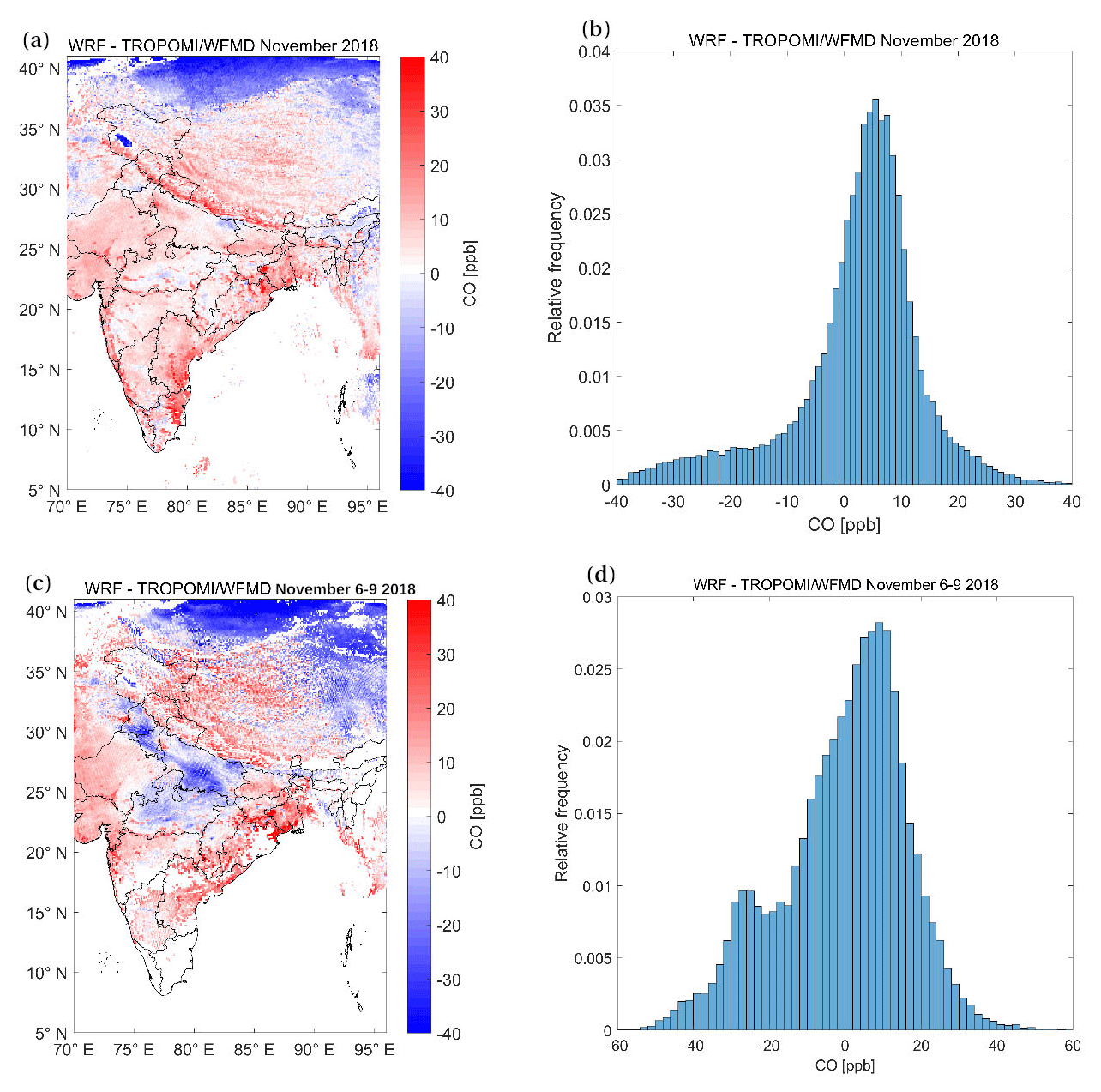
Figure 4 (a) Differences in CO total column mixing ratios (WRF – TROPOMI/WFMD) averaged over the month of November 2018. (b) Histogram of the differences. (c) Same as panel (a) but restricting the period to 6–9 November 2018. (d) Same as panel (b) but restricting the period to 6–9 November 2018.

During the biomass burning period, the model underestimates (by about 10–15 ppb) the enhancement over Punjab and some central parts of Uttar Pradesh, while overestimating (by about 15–20 ppb) enhancements over the eastern parts of IGP, including West Bengal and some parts of Bihar. Daily retrievals of TROPOMI/WFMD and the corresponding simulations for the biomass burning period are shown in Fig. 5. An enhanced XCO is reported in both observations and simulations over the state of Punjab, starting from 6 November and gradually increasing in the following days. During this period, the plume is seen to be partly transported in a southeasterly direction along the regions of Delhi and Agra. Over the IGP there exists an overall slight underestimation by WRF in comparison to TROPOMI during this period, with a mean model-to-observation difference of −2.7 ppb.

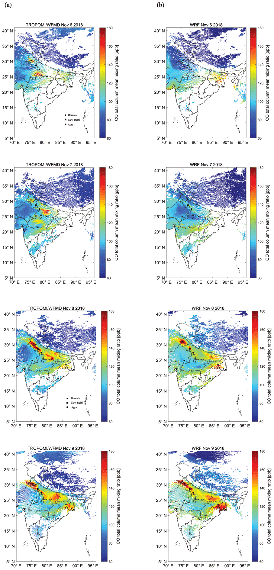
Figure 5 (a) Daily column CO observations from TROPOMI/WFMD and (b) the co-located WRF simulation for 6–9 November 2018.

Figure 6 shows the temporal evolution of the CO concentration in three cities (Barnala, New Delhi, and Agra) located along the transport pathway of pollution. The data are averaged in a 100 km × 100 km square around the centre of each city. During the biomass burning period, the XCO over Barnala (Punjab) shows a steady positive increment with time, with a peak on 9 November with a value of approximately 165 ppb. Both observations and simulations suggest a southeasterly transport of this plume, which increases the CO concentration over Delhi and Agra during 8 and 9 November. Over Delhi, the TROPOMI/WFMD XCO reached a maximum on 8 November, while modelled CO showed a delay with a maximum concentration on 9 November. On 9 November, the observation shows more dispersed XCO over Delhi towards the southeasterly direction in comparison with model simulations. Over Agra, which is located far away from the pollution hotspot but along the transport pathway, an increase in XCO, which is consistent with that over the other two cities, is found.

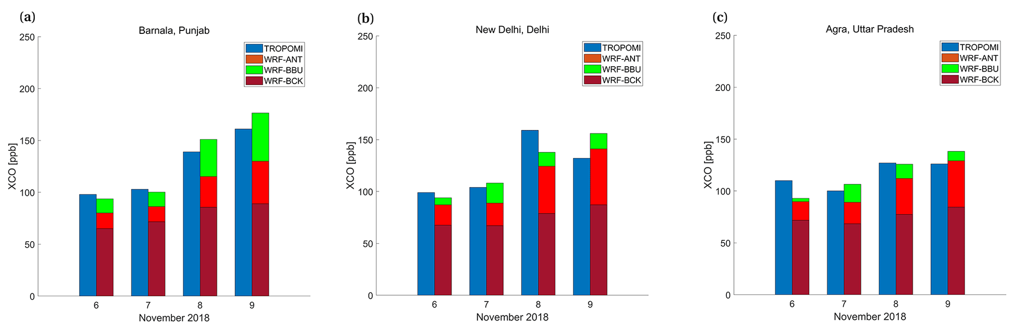
Figure 6 Carbon monoxide (CO) total column mixing ratios over (a) Barnala, (b) New Delhi, and (c) Agra for individual days from 6–9 November 2018.

Based on VIIRS AOD (aerosol optical depth) and WRF–Chem simulations using different chemical and meteorology boundary conditions and biomass burning emissions, Roozitalab et al. (2021) assessed the model performance over the IGP region during an intensive fire period in November 2017 and reported an underestimation of AODs for the entire IGP region, except for Punjab. Furthermore, Kumar et al. (2020) found a considerable impact of uncertainties in the WRF meteorology on simulated PM_2.5 concentrations over IGP during the crop residue burning period in November 2017. Note that our study also reports a slight underestimation of WRF compared to TROPOMI CO observations over IGP during the biomass burning period. Though we cannot directly compare AOD and/or PM_2.5 results during November 2017 from previous studies with our CO simulations during November 2018, the results indicate shortcomings in the model that can be refined by better representation of atmospheric transport (including model initialization) and emission.

The details in Table 4 confirm the minimal impact of the differences in satellite retrieval algorithms on our results. This analysis suggests a promising usage of TROPOMI observations for understanding the details of hotspot emissions and the distribution of transport. The model is able to capture many of these spatial and temporal patterns, supporting the potential use of WRF via inverse modelling to infer hotspot emissions using column measurements.

5.3.2 Agreement with ground-level observations

Figure 7 shows the model evaluation with ground-level measurements over the regions IGP, Delhi, and Punjab for a period from 3 to 20 November 2018. The location of ground-level measurement stations used for this study is shown in Fig. 8. The entire month is not used here due to the existence of data gaps from several stations. Taking various ground-based stations over the IGP, Delhi, and Punjab, we see an overall agreement between the model and measurements, with a correlation coefficient of 0.6 (for the IGP), 0.6 (Delhi), and 0.41 (Punjab). Among these three study regions, a lower correlation is found for the Punjab region in which measurement sites are very close to the biomass burning hotspots, therefore showing a larger variability associated with biomass emissions compared to other stations. These variations are not fully reproduced by the model, resulting in lower correlations over the Punjab region. Though the model is able to follow the temporal variation in the surface-level CO concentrations, overall underestimations of 9 and 54 ppb are found for Punjab and Delhi. For the IGP region, the model underestimates the observed enhancements considerably, resulting in a mean bias of 162 ppb. The observed underestimation of WRF can be attributed to the local source enhancements at the ground-level stations, which are located close to the cities. For the Punjab region, the model CO surface concentration shows the influence of biomass burning, starting from 6 November with a maximum of 800 ppb on 8 November. Unlike the Punjab region, the concentration patterns over Delhi and the IGP show a steadily increasing trend from 6 to 13 November, with a subsequent reduction in mixing ratios for the remaining days. Among these study regions during this period, the lowest and highest surface CO levels are observed over the regions of Punjab (mean – 500 ppb) and Delhi (mean – 1500 ppb), respectively. Except for Punjab, we see better mean bias when excluding nighttime values (21 ppb for Delhi and 141 ppb for the IGP region), as the uncertainty from mixing height simulations is larger during nighttime compared to daytime. Surprisingly the overall underestimation increased in Punjab when using only daytime values, indicating a considerable underestimation of local emission sources, likely from the biomass emission inventory. Note that the GFAS fire emissions may be underestimated (Mota and Wooster, 2018). The GFAS fire emissions are partly based on the MODIS satellite instrument, and the limited resolution of the instrument misses many small fires, including biomass burning over India (Cusworth et al., 2018). A comparison of post-monsoon fire CO emissions over Punjab and Haryana, as estimated from five global inventories for the period from 2003 to 2016, indicates the limitation of satellite-derived fire products and the associated uncertainties in the CO fire emissions (Liu et al., 2019). Overall, the results show that the model simulation, at a high spatial resolution, is capable of capturing the CO enhancement and reduction pattern at most of the stations; however, there is a non-trivial mean bias which can be attributed to issues with simulating transport (including the emission release height) and PBL dynamics in WRF as well as the variability in emission fluxes (both EDGAR and GFAS), which is likely to not be sufficiently well represented in the emission inventories used.

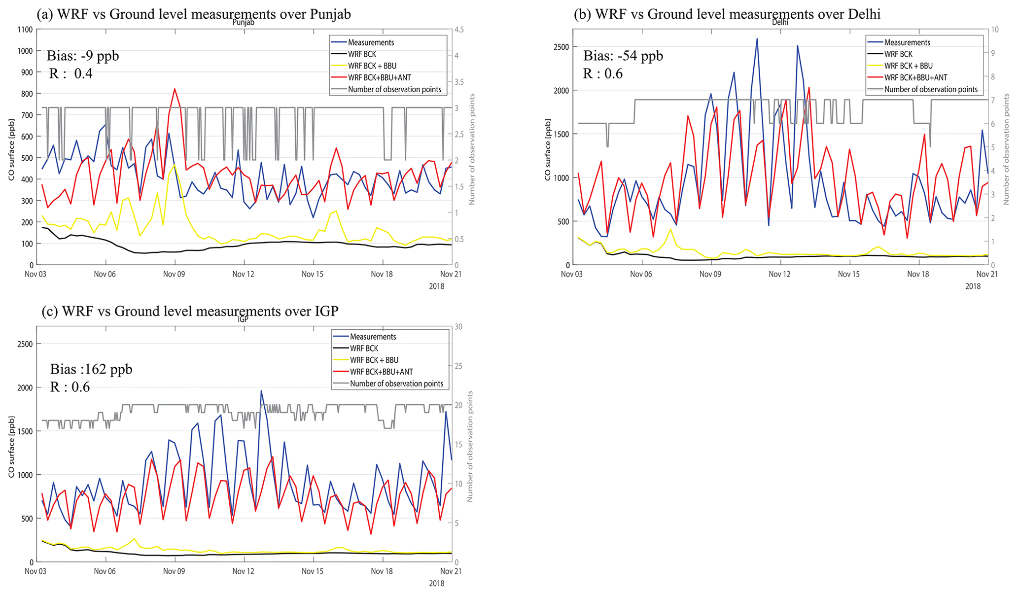
Figure 7 Ground-level CO measurements and WRF model simulations for the period 3–20 November 2018 over (a) the IGP region, (b) Delhi, and (c) Punjab. Note that different y-axis scale ranges are used in the panels for a better visualization of the signals.

Figure 8 Map showing the locations of sites used for model evaluation. The yellow contour represents the IGP region. The inset shows the broader region for context.

5.4 Contribution of different sources to the observed concentration

To further investigate the contribution of different emission sources to the observations, we use the tagged tracer option in WRF and separate the contributions from different sources, as shown in Figs. 6 and 7. Note that the signals contributing to satellite observations are difficult to disentangle without underlying assumptions or the availability of multi-tracers such as CO and nitrogen oxides and the following: NO_x and NO${}_y^{*}$ (NO${}_y^{*}$ includes NO_x, peroxyacetyl nitrate (PAN), organic nitrates, nitric acid (HNO₃), and dinitrogen pentoxide (N₂O₅; e.g. Wang et al., 2002). The relative contributions of different emission sources and processes to the WRF CO column, as summarized in Table 4, clearly indicate the dominance of anthropogenic signals over biomass burning signals on the XCO enhancements (see Figs. S1 and S2 in the Supplement). The significant impact of background signal, owing to the advection from the domain boundary throughout the column, indicates the influence of far-field fluxes and large-scale transport patterns on column CO (see Fig. 6). During the biomass burning period, there exists a considerable contribution of biomass burning emissions to the column mixing ratios, particularly over the Punjab region (14 %). Relatively low contributions of biomass burning signals to the column in Delhi and the IGP compared to Punjab indicates the dominant contribution of surface CO emission to the column in Punjab, which is where the biomass emissions originated. It also suggests the possibility of less dilution of surface emissions during wintertime, enhancing the total column mixing ratios. The effect of advected biomass burning signals in terms of their contribution to the column can be seen over Delhi (12 %); however, this effect becomes smaller in the IGP (5 %) due to further dispersion.

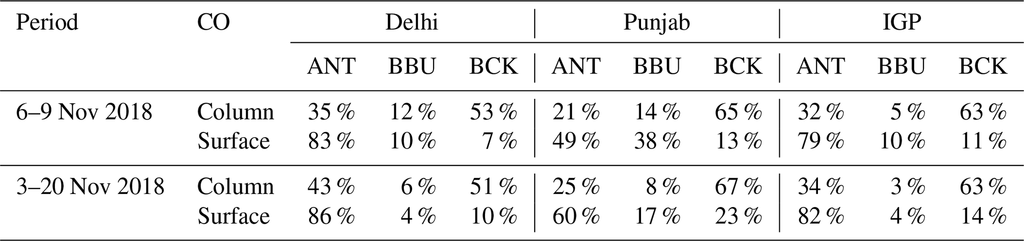
The diurnal variation in the surface-level CO concentration pattern is due to the diurnal variation in the planetary boundary layer height (PBLH) combined with strong sources of CO at the surface. The contribution from emissions sources over the Delhi, IGP, and Punjab regions for the period of 3–20 and, specifically, 6–9 November are also summarized in Table 5. For all regions, the influence of background CO concentrations to the surface-level CO observed variability is minimal, as expected (see Fig. 7). The background influence is expected to be smaller for surface CO in urban areas, where the CO fraction from local anthropogenic emissions dominates the background signals. At ground level in Delhi and the IGP, a detectable enhancement in surface CO due to fire CO is found only during 6–9 November. During this period, the average contribution of biomass burning to the ground-level concentration is 10 %, while the anthropogenic contribution is 79 %–83 %. During 3–20 November over Delhi, however, the average contribution from fire dropped to 4 % compared to 85 % in the case of the anthropogenic contribution.

Table 5 Contributions from different emissions sources to the CO concentration between 6–9 and 3–20 November 2018. Abbreviations ANT, BBU, and BCK represent anthropogenic, biomass burning, and background signals, respectively (see Sect. 3).

To examine the impact of missed active fires on our WRF results, we perturb GFAS fire emissions by a factor of 50 % and quantify how this perturbation affects the size of the anomaly in CO mixing ratios over the IGP region. Note that VIIRS detected ∼ 20 % more active fires during the post-monsoon season over Punjab and Haryana. Using the perturbed GFAS emissions, we estimate that the relative increase in modelled XCO contribution arises from increased biomass emissions. With the increased emissions, we see an increment of XCO contribution, ranging approximately from 5 to 25 ppb, during biomass burning period over IGP region, mostly over Punjab, Haryana, and Delhi (see Figs. S3 and S5). As for the model observation performance statistics, a slight improvement is found for XCO over IGP region with this perturbed simulation (see Table S1).

For allocating small fires over the model domain, we use the GFED4s fire product, including fire fractions stemmed from the small fire-burned area. The small fire boost in GFED4s is calculated based on active fire hotspots and burned area observations from MODIS surface reflectance (Randerson et al., 2012). The difference in fire emission fields in GFED4s, relative to GFAS, is derived over the model domain and is applied to WRF to quantify the fire CO contribution that also includes small fires. While including small fires based on GFED4s has improved the model observation mean bias over IGP region for surface CO mixing ratio during biomass burning period, we see a minimal improvement for XCO (see Table S1). Enhancing the fire emission by incorporating small fires resulted in an overall increment of XCO concentration ranging from 20 to 40 ppb; however, most of the contributions arising from small fires are seen only over Punjab and some parts of Haryana (see Figs. S3 and S5). Based on GFED4s, we quantify the effect of small fires on the modelled atmospheric CO plumes. The addition of small fires contributed to an increment of 12.2 % surface CO over Punjab and Haryana, and the small fire contribution is reduced to 8.6 % and 4.3 % over Delhi and IGP, respectively. In the case of XCO, there exists only a minimal impact of small fires on mixing ratios, which are estimated to be 2.5 % over Punjab and Haryana, 1.4 % over IGP, and 0.8 % over Delhi. The difference in the contribution of small fires between surface CO and XCO can be explained by the meteorology conditions that prevailed (see Sect. 5.5).

Overall, our findings suggest that the enhanced CO levels during pollution episodes over Delhi and the greater part of IGP are affected by biomass burning. However, a more significant contribution comes from anthropogenic emissions. Unlike the surface CO mixing ratios, the majority of the column CO mixing ratio is contributed by the background signal. A recent study conducted by Dekker et al. (2019) concluded that there exists an underestimation in GFAS fire emission data over the Indian region. This is also supported by our study in which we find that the underestimation of the total CO concentration in Punjab during biomass burning period and a part of this model observation mismatch can be attributed to the underestimation of modelled fire CO contribution. Over the Punjab region, biomass burning played a significant role in determining the ground-level CO measurements, especially during 6–9 of November during which enhanced fire activities occurred. This has contributed considerably to the column mixing ratio that is detected by TROPOMI. On average, for 3–20 November, 17 % of the total ground-level CO concentration over the Punjab region is on account of fire CO emission, whereas for 6–9 November the share is about 38 %.

5.5 Effect of meteorology

Usually pollution episodes during winter are the result of meteorological conditions due to low wind speed and a shallow boundary layer (PBL height). To further analyse the effect of meteorological conditions, we use WRF-simulated meteorology due to the lack of observations of wind and PBL height in this region. An inter-model comparison of WRF meteorology with corresponding variables from reanalysis data provided by Modern-Era Retrospective Analysis for Research and Applications, version 2 (MERRA-2) is performed to assess the overall agreement (see Table S2 and Fig. S6). Note that MERRA-2 is an assimilation product at an approximate spatial resolution of 0.5^∘ × 0.625^∘, publicly available online at https://gmao.gsfc.nasa.gov/reanalysis/MERRA-2/ (last access: 14 January 2021). More information on MERRA-2 and the assimilation system can be seen in Gelaro et al. (2017). Figure 9 demonstrates the influence of the PBL height and surface-level wind speed to the observed CO level. We found a negative correlation of CO with modelled PBLH (−0.83 – IGP; −0.73 – Delhi; −0.56 – Punjab) and wind speed (−0.40 – IGP; −0.62 – Delhi; −0.24 – Punjab) for November 2018. Similar correlations of CO with modelled PBLH (−0.87 – IGP; −0.83 – Delhi; −0.65 – Punjab) and wind speed (−0.46 – IGP; −0.70 – Delhi; −0.26 – Punjab) exist for the biomass burning time period of 6–9 November 2018. A strong negative relation between PBL height and CO level is seen, indicating the impact of meteorology on the diurnal variation of surface-level CO concentration. Among the regions, a less negative correlation of CO with PBLH and wind speed is observed for Punjab. It suggests that, when compared to Delhi and the IGP, the surface-level CO variation over the Punjab region cannot be explained by meteorology alone. Here the local emission activities, such as biomass burning, explain more of the variability in surface-level CO. A gradual increase in surface CO levels was observed from 3 to 13 November during which an overall decrease in PBL height and surface-level wind speed took place. The highest CO values around Delhi were found during 11–13 November, just before the winds and PBL height were increasing.

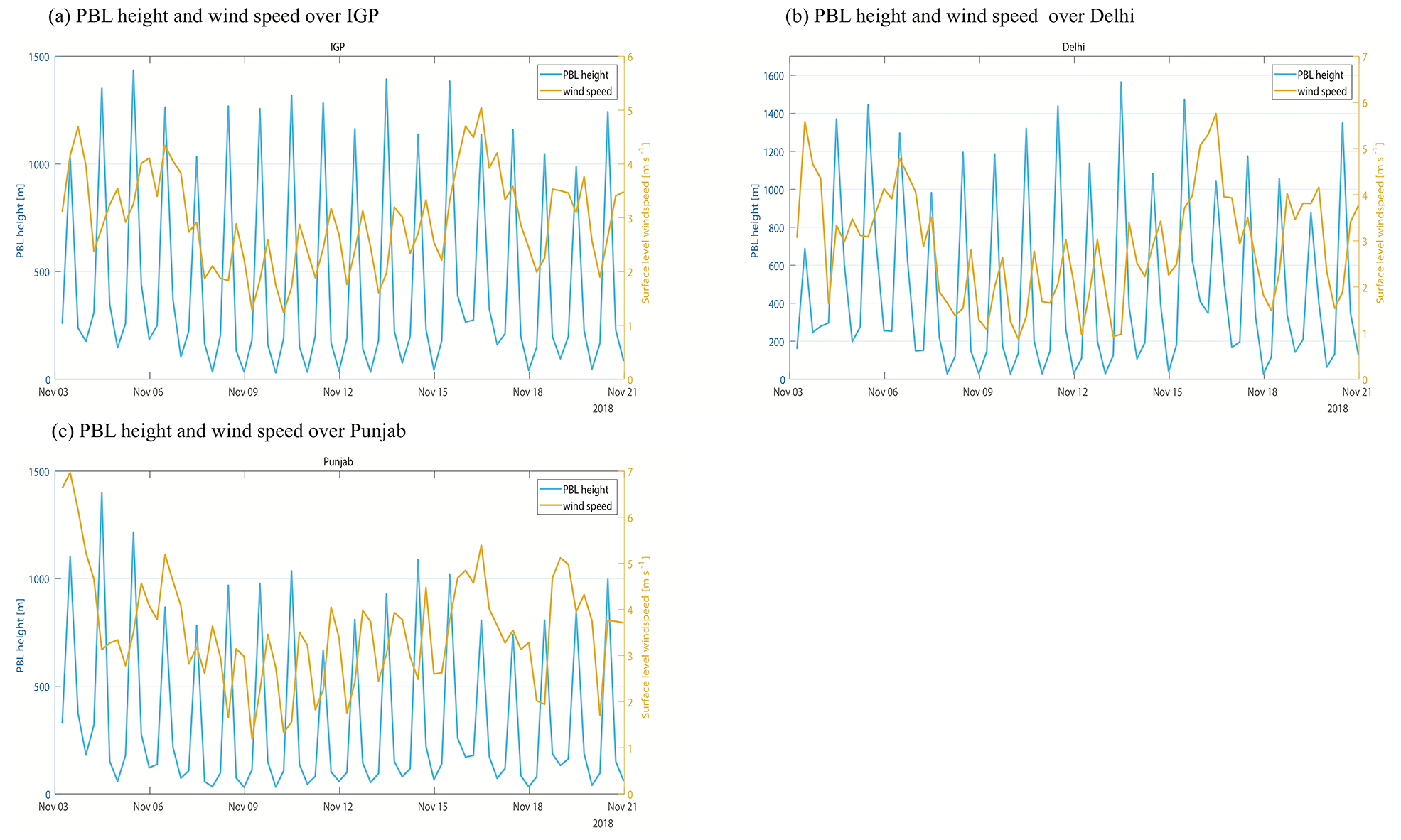
Figure 9 PBL height and surface-level wind speed from WRF model simulations for a period of 3–20 November 2018 over (a) the IGP region, (b) Delhi, and (c) Punjab.

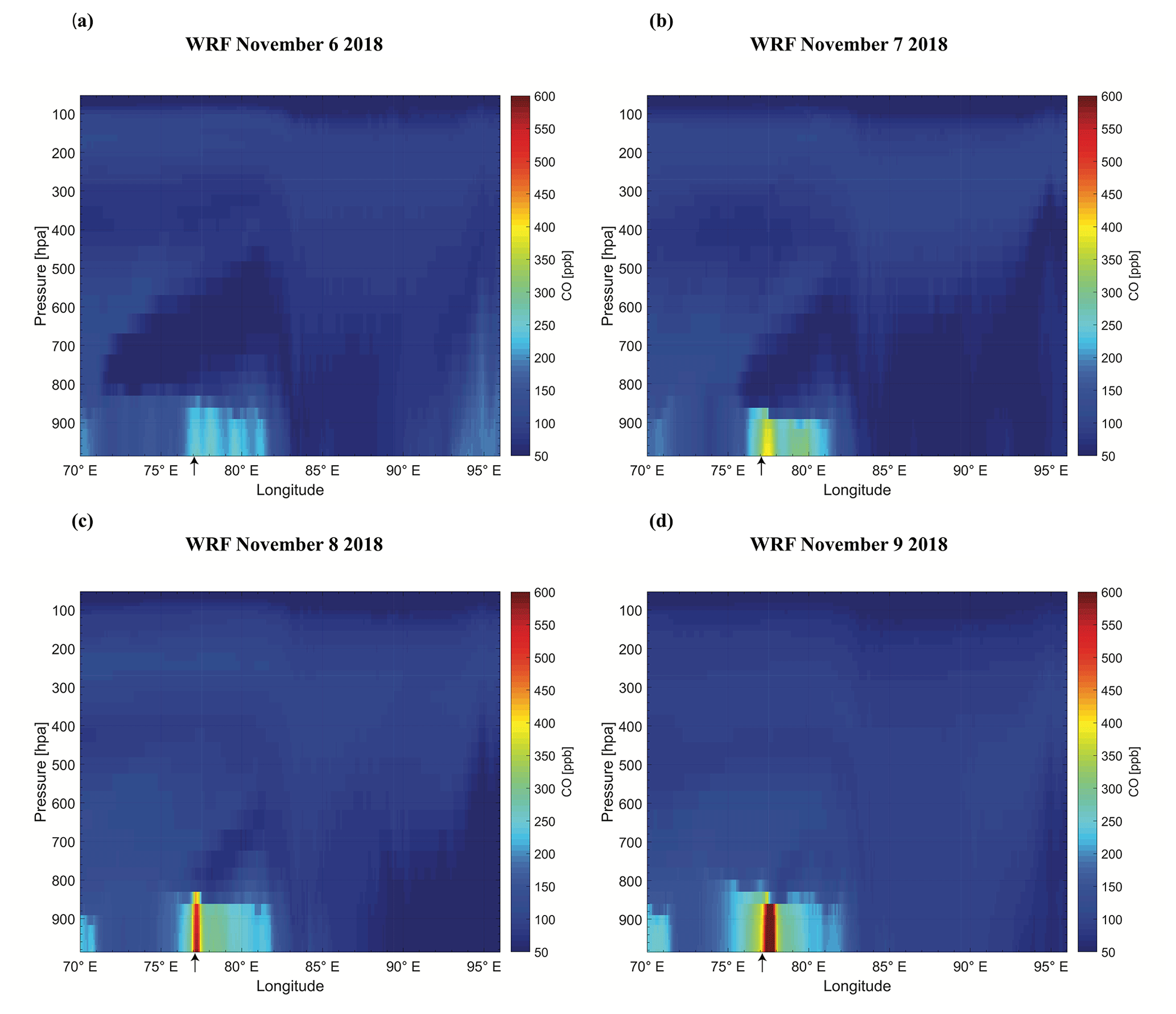
Figures 10 and 11 provide transport patterns involving the vertical distribution of CO biomass burning contribution and total CO mixing ratio, respectively, during the biomass burning period. Vertical cross sections show an impact of fire emission over Delhi during the biomass burning period (40 to 120 ppb), peaking its boundary layer CO contribution (>110 ppb) on 7 November (Fig. 10). On the other hand, the total CO shows peak values (>550 ppb) on 9 November, indicating a significant additive contribution from anthropogenic fluxes, in addition to biomass burning, together with the winter meteorology conditions that prevailed over the region (see Fig. 11). A consistently low PBL height can be clearly seen during these days, which traps CO plumes in the lower boundary layer due to less extent of vertical mixing. These findings suggest that the meteorological conditions have a large impact on the surface-level CO concentration, especially over the IGP and Delhi. Our results are consistent with Dekker et al. (2019), who identified that the meteorological conditions contributed significantly to the enhancement of CO mixing ratios at the ground level during November 2017. Similarly, Kariyathan et al. (2020), by using a-temporal emission fields and a Lagrangian modelling framework, found a considerable impact of meteorological conditions during November 2017 that contributed to the enhancements of trace gases over Delhi. Together with strong emissions (anthropogenic and biomass burning), they found that these enhancements could be several orders of magnitude higher compared to other seasons.

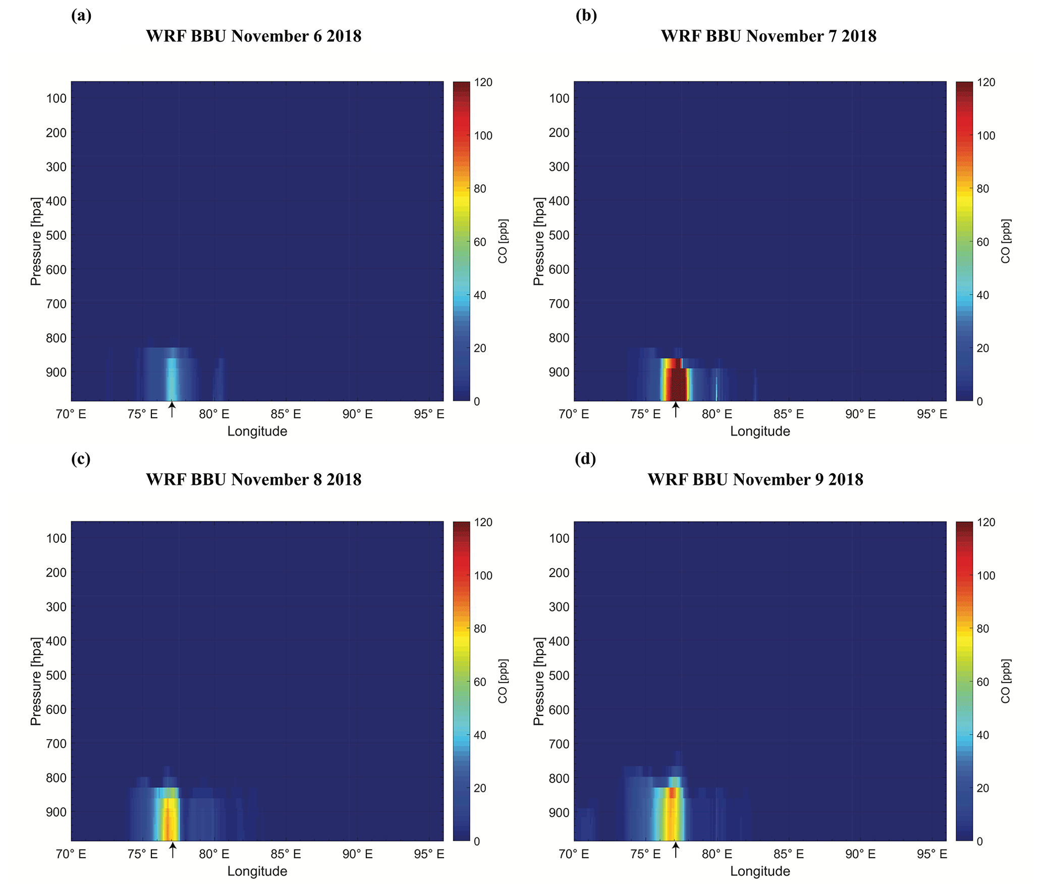
Figure 10 Vertical cross section of the CO mixing ratio that arises from biomass burning emissions during 6–9 November 2018. Cross sections are over Delhi at 13:30 (local time). The black arrow indicates the location of Delhi.

Figure 11 Same as Fig. 10 but showing total CO distribution.

6 Conclusions

The TROPOMI on board the European Space Agency's S5P mission provides shortwave infrared measurements of CO with a daily global coverage and a high spatial resolution of 7×7 km². These high-density and high-accuracy CO column observations enable us to investigate high CO pollution episodes over India, which otherwise would not have been possible at this spatial resolution. In this study, we demonstrate the usefulness of TROPOMI CO column observations for detecting and analysing local CO enhancement over India during winter 2018, employing WRF at a resolution comparable to TROPOMI to aid in the interpretation of the data. The GFAS biomass burning emission product shows a substantial amount of fire CO emitted from various parts of India during the year 2018. Over the IGP, the fire CO emission shows an apparent monthly variation, with a higher emission during the post-monsoon time compared to the pre-monsoon period. A large amount of fire CO emissions is reported over the state of Punjab within the short period of 6–9 November 2018. Consistent with the emission data, TROPOMI XCO shows a clear enhancement during November, not only over the fire emission hotspots but also along the western parts of the IGP, including the capital of India, Delhi.

To further analyse the causes of these enhancements, we used simulations generated by WRF. A similar study conducted by Dekker et al. (2019) also utilized WRF to identify the sources contributing to the high pollution event in northern India during 2017 but used preliminary TROPOMI data generated with the SICOR algorithm. The present study uses both fossil fuel emissions data based on EDGAR (version 4.3.2), with hourly variations, and biomass burning emissions data based on GFAS fire CO emissions. If WRF reproduces the transport sufficiently well, the mismatch between the simulations and observations is mostly caused by uncertainties in the prior emission fluxes (EDGAR and GFAS) due to the linear dependence of the CO concentrations on the source strength of the emissions. To evaluate the simulated CO fields with the observed CO columns, we applied the TROPOMI/WFMD averaging kernel to the corresponding model profile, taking into account the vertical sensitivity of the satellite measurement. Overall, we find a good agreement between WRF and TROPOMI/WFMD.

Our analysis shows that daily observations from TROPOMI allow pollution transport from the emissions hotspots to be captured. As an example, we analysed the pollution transport from the fire emissions hotspots over northern India during the enhanced burning period of 6–9 November. The TROPOMI/WFMD XCO level started to rise over the fire emission hotspots from 6 November and gradually increased during the following days. Both TROPOMI/WFMD and model simulations show the transport of CO polluted air masses towards the northeastern part of the IGP along with the capital city of Delhi. Due to this pollution transport, the CO concentration level in the cities along the transport pathway shows CO enhancements. A similar transport pattern is also observed in our WRF model simulation. This supports the reliability of the WRF transport simulation and suggests the potential of using WRF to estimate CO emission via flux inversions. The good agreement between TROPOMI/WFMD and TROPOMI/SICOR retrievals over India confirms the robustness of our findings irrespective of the differences in the retrieval algorithm. For the further evaluation of WRF with surface measurements, we used ground-level CO measurements from the stations along the IGP for the period of 3–20 November 2018. Over these regions, the surface CO showed a steadily increasing trend from 6 to 13 November, followed by a reduction in mixing ratio in the following days. Among these study regions, the lowest and highest surface CO level was observed over the regions Punjab and Delhi respectively.

We answer the five questions raised in the introduction as follows: (1) the TROPOMI XCO shows a clear enhancement during the stubble burning period over the fire emission hotspots but also along the western parts of the IGP, including the national capital of India, Delhi. The detected XCO level over most parts of the IGP was about 40 ppb higher than in other parts of India. (2) In terms of regional fire CO contribution, in most parts of India, the fire CO emissions peak during the pre-monsoon period (76 %) compared to the post-monsoon period (24 %). Fire activities over northeastern India (NEI) made a significant contribution (57 %) to emissions during pre-monsoon months, while the IGP contributed only about 5 %. Central (CI) and southern regions (SI) of India add about 33 % towards the pre-monsoon fire CO emissions. IGP contributed about 73 % of the country's total fire CO emissions during the post-monsoon period. A large number of fire CO emissions is reported over the state of Punjab within the short period of 6–9 November 2018. (3) Comparing model simulations with observations, we find a good agreement between WRF and TROPOMI/WFMD, with a mean difference of 7 ppb, a standard deviation of 8 ppb, and a spatial correlation coefficient of 0.87. The comparison of WRF CO at surface level with ground-level CO measurements from the stations along the IGP for the period of 3–20 November 2018 shows a less agreement compared to the values for XCO, with a correlation coefficient of 0.6 (for the IGP), 0.6 (Delhi), and 0.41 (Punjab). (4) The response of column CO to the surface biomass emission was clearly visible during the enhanced burning period. The CO level started to rise over the fire emission hotspots from 6 November and gradually increased during the following days (see Fig. 5). (5) Compared to anthropogenic emission sources, our results imply a minimal role of biomass burning in terms of its contribution to both column and surface enhancements, except for the state of Punjab during the high pollution episodes. This is also consistent with Dekker et al. (2019), who concluded that the low wind speeds and shallow atmospheric boundary layers were the most likely causes for the temporal accumulation and subsequent dispersion of CO during the biomass burning period in November 2017.

Overall, comparing our results with Dekker et al. (2019), we can infer the significant role of atmospheric dynamics and anthropogenic emissions in producing exorbitant level of pollutants and trace gases during every winter in northern India. While these anthropogenic urban sources (e.g. road traffic, residential usages, such as cooking and heating by solid fuels, industries, including coal-fired kilns, and power plants) are primarily responsible for the CO enhancement in winter months, there exists a non-trivial fraction of contribution from biomass burning activities in Punjab and nearby locations for a short duration of time. The variation in surface-level CO concentrations is found to be influenced significantly by the meteorological parameters such as PBL height and surface-level wind speed. Our results show a clear influence of atmospheric transport, leading to a complex CO enhancement pattern. This demonstrates the need for high-resolution models in the interpretation of TROPOMI observations in order to obtain more insight into the pollution transport and deduce causes for the observed enhancements (and resulting poor air quality) over India.

In an effort to minimize the pollution episodes, a robust evaluation of emissions inventories and their trends is vital, particularly in light of uncertainties in existing emission sources, and the limited availability of appropriate emissions estimates in different emission sectors. Studies identifying the emissions hotspots and understanding their transport patterns, such as those carried out in Dekker et al. (2019) and in this work, are thus important for further decision-making for controlling emissions. While WRF is able to reproduce observations reasonably well, the model errors are not negligible when utilizing TROPOMI observations for emission estimates. Nevertheless, we emphasize the importance of taking rigorous policy measures to reduce residential and commercial emissions in addition to measures already being taken in the agricultural sectors (e.g. the implementation of second-generation direct seeders, such as the Happy Seeder, which facilitate sowing under heavy stubble conditions, thereby avoiding the need for residue burning; NAAS, 2017). The future task involves the implementation of appropriate inverse techniques suitable for flux inversion of spatially resolved sources of CO emissions over India.