the Creative Commons Attribution 4.0 License.
the Creative Commons Attribution 4.0 License.
 | 18 Mar 2021
Simulations of anthropogenic bromoform indicate high emissions at the coast of East Asia
Josefine Maas
Susann Tegtmeier
Birgit Quack
Jonathan V. Durgadoo
Arne Biastoch
Bromoform is the major by-product from chlorination of cooling water in coastal power plants. The number of power plants in East and Southeast Asian economies has increased rapidly, exceeding mean global growth. Bottom-up estimates of bromoform emissions based on few measurements appear to under-represent the industrial sources of bromoform from East Asia. Using oceanic Lagrangian analyses, we assess the amount of bromoform produced from power plant cooling-water treatment in East and Southeast Asia. The spread of bromoform is simulated as passive particles that are advected using the three-dimensional velocity fields over the years 2005/2006 from the high-resolution NEMO-ORCA0083 ocean general circulation model. Simulations are run for three scenarios with varying initial bromoform concentrations based on the range of bromoform measurements in cooling-water discharge. Comparing the modelled anthropogenic bromoform to in situ observations in the surface ocean and atmosphere, the two lower scenarios show the best agreement, suggesting initial bromoform concentrations in cooling water to be around 20–60 µg L−1. Based on these two scenarios, the model produces elevated bromoform in coastal waters of East Asia with average concentrations of 23 and 68 pmol L−1 and maximum values in the Yellow Sea, Sea of Japan and East China Sea. The industrially produced bromoform is quickly emitted into the atmosphere with average air–sea flux of 3.1 and 9.1 , respectively.
Atmospheric abundances of anthropogenic bromoform are derived from simulations with the Lagrangian particle dispersion model FLEXPART based on ERA-Interim wind fields in 2016. In the marine boundary layer of East Asia, the FLEXPART simulations show mean anthropogenic bromoform mixing ratios of 0.4–1.3 ppt, which are 2–6 times larger compared to the climatological bromoform estimate. During boreal winter, the simulations show that some part of the anthropogenic bromoform is transported by the northeasterly winter monsoon towards the tropical regions, whereas during boreal summer anthropogenic bromoform is confined to the Northern Hemisphere subtropics. Convective events in the tropics entrain an additional 0.04–0.05 ppt of anthropogenic bromoform into the stratosphere, averaged over tropical Southeast Asia. In our simulations, only about 10 % of anthropogenic bromoform is outgassed from power plants located in the tropics south of 20∘ N, so that only a small fraction of the anthropogenic bromoform reaches the stratosphere.
We conclude that bromoform from cooling-water treatment in East Asia is a significant source of atmospheric bromine and might be responsible for annual emissions of 100–300 Mmol of Br in this region. These anthropogenic bromoform sources from industrial water treatment might be a missing factor in global flux estimates of organic bromine. While the current emissions of industrial bromoform provide a significant contribution to regional tropospheric budgets, they provide only a minor contribution to the stratospheric bromine budget of 0.24–0.30 ppt of Br.
- Article
(5425 KB) - Full-text XML
-
Supplement
(624 KB) - BibTeX
- EndNote


Power plants require cooling water to regulate the temperature in the system. As their demand for cooling water is very high, power plants are often located at the coast to profit from an unlimited water supply. Seawater, however, needs to be disinfected to prevent biofouling and to control pathogens in effluents. The usual disinfection method, chlorination, is known to generate a broad suite of disinfection by-products (DBPs) including trihalomethanes, halogenated acetic acids and bromate (e.g. Helz et al., 1984; Jenner et al., 1997). The generally proposed mechanism for generating DBPs is the reaction of oxidants such as chlorine and ozone with organic and inorganic substances, such as bromide (Br−) and iodide (I−), in the water via the formation of hypobromous (HOBr) and hypoiodous (HIO) acid (Allonier et al., 1999; Khalanski and Jenner, 2012). Discharge of DBPs within the cooling-water effluent can be harmful to the local ecosystem in combination with temperature and pressure gradients (Taylor, 2006). The composition and amount of generated DBPs depend on many factors including the type and concentration of the injected oxidant and the chemical characteristics of the treated water such as salinity, temperature and amount of dissolved organic matter (Liu et al., 2015). Cooling-water effluents regularly involve the discharge of large water volumes into the marine environment (Khalanski and Jenner, 2012). This water is often warmer than the surrounding waters, and its decreased density means it stays at the sea surface. Chemicals such as DBPs contained in cooling water are likely to spread laterally across the sea surface, which facilitates air–sea gas exchange for volatile DBPs.
One of the major DBPs is bromoform (CHBr3), a halogenated volatile organic compound. Bromoform is also naturally produced in the ocean by macroalgae and phytoplankton and is the largest source of organic bromine to the atmosphere (Quack and Wallace, 2003). Current estimates of bromoform emissions show large variations and suggest a global contribution to atmospheric bromine (Br) of 0.5–3.3 Gmol Br a−1 (Engel and Rigby, 2018). Bottom-up bromoform emission estimates based on statistical gap filling of observational surface data suggest in general smaller global fluxes when compared to other approaches. The bottom-up approach from Ziska et al. (2013) uses surface ocean and atmosphere measurement collected in the HalOcAt (Halocarbons in the Ocean and Atmosphere) database (https://halocat.geomar.de/, last access: 1 March 2021) to estimate bromoform emissions of 1.5 Gmol Br a−1. Based on physical and biogeochemical characteristics of the ocean and atmosphere, the data are classified into 21 regions and extrapolated to a regular grid within each region. Top-down bromoform emission estimates, on the other hand, are based on global model simulations adjusted to match available aircraft observations (e.g. Butler et al., 2007; Liang et al., 2010; Ordóñez et al., 2012). They are, in general, a factor of 2 larger than bottom-up emission estimates. Individual ship cruises, aircraft campaigns and modelling studies have demonstrated a large spatio-temporal variability of bromoform in surface water and air (e.g. Fiehn et al., 2017; Fuhlbrügge et al., 2016; Jia et al., 2019). These pronounced variations combined with the poor temporal and spatial data coverage are a major challenge when deriving reliable emission estimates and may explain the large deviations between bottom-up and top-down estimates. Geographical regions with poor data coverage might not be well represented in the global emission scenarios. Furthermore, the anthropogenic input of bromoform might be underestimated for large industrial regions (Boudjellaba et al., 2016).
With an atmospheric lifetime of about 2–3 weeks, bromoform belongs to the so-called very short-lived substances (VSLSs) (Engel and Rigby, 2018). Once bromoform is photochemically destroyed in the atmosphere, it can deplete ozone by catalytic cycles (Saiz-Lopez and von Glasow, 2012) or change the oxidising capacity of the atmosphere by shifting HOx ratios towards OH (Sherwen et al., 2016). In the tropics, VSLSs such as bromoform can be entrained into the stratosphere (e.g. Aschmann et al., 2009; Liang et al., 2010; Tegtmeier et al., 2015) and contribute to stratospheric ozone depletion (Hossaini et al., 2015). Stratospheric entrainment of trace gases with very short lifetimes is most efficient in regions of strong, high-reaching convective activity such as the western Pacific and Maritime Continent (e.g. Pisso et al., 2010; Marandino et al., 2013). The Asian summer monsoon represents another important pathway to the lower stratosphere (e.g. Randel et al., 2010), entraining mostly Southeast Asian planetary boundary layer air. The monsoon also has the potential to include VSLSs emitted from the Indian Ocean and Bay of Bengal (Fiehn et al., 2017, 2018b). Model simulations suggest that the monsoon circulation transports the oceanic emissions towards India and the Bay of Bengal, from where they are convectively lifted and reach stratospheric levels in the southeastern part of the Asian monsoon anticyclone. The stratospheric bromine injections from the tropical Indian Ocean and western Pacific depend critically on the seasonality and spatial distribution of the emissions (Fiehn et al., 2018a). Model studies based on bottom-up emission estimates indicate global bromoform maxima over India, the Bay of Bengal, and the Arabian Sea as well as over the Maritime Continent and western Pacific (Tegtmeier et al., 2020a). While aircraft measurements in the western Pacific have confirmed high concentrations of bromoform (Wales et al., 2018), the role of the Asian monsoon as an entrainment mechanism for VSLSs has not been confirmed yet due to the lack of observations in this region.
Quantifying the contribution of bromoform to tropospheric and stratospheric bromine budgets requires reliable emission estimates that include natural and anthropogenic sources. Industrially produced bromoform will spread in the marine environment once the treated water is released and will be emitted into the atmosphere together with naturally produced bromoform. Atmospheric and oceanic measurements cannot distinguish between naturally and industrially produced bromoform, and all the top-down and bottom-up emission estimates discussed above potentially include the latter already. A first comparison of natural and industrial bromoform sources from Quack and Wallace (2003) concluded a negligible global contribution of 3 % man-made bromoform. Their estimate was based on measurements of bromoform in disinfected water (80 nmol L−1) from European power plants and cooling-water use and projections of the global electricity production. In the meantime, the global electricity production has increased by almost 50 % from 16 700 TWh in 2003 (IEA, 2005) to 25 000 TWh in 2016 (IEA, 2018). Furthermore, new measurements of bromoform in disinfected cooling water have become available, suggesting potentially higher concentrations of up to 500 nmol L−1 (Padhi et al., 2012; Rajamohan et al., 2007; Yang, 2001). Emerging economies in East Asia, such as China and India, have experienced a massive growth over the last years, exceeding the global economic growth. As the existing estimate of industrially produced bromoform is outdated, updated estimates taking into account new measurements are required to assess the impact of anthropogenic activities on the production and release of brominated VSLSs as well as their contribution to stratospheric ozone depletion.
We will derive a new bottom-up VSLS emission estimate for East and Southeast Asia by quantifying anthropogenic contributions to bromoform production. We will use available cooling-water measurements to predict oceanic and atmospheric bromoform concentrations in regions of extensive industrial activities. Based on comparisons to available ocean surface and atmosphere measurements, we will evaluate our predictions and discuss implications for an atmospheric bromine budget as well as future research needs. As 50 % of the global coastal cooling water is produced in East and Southeast Asia, we define these areas as our study region. We identify locations of high industrial activity along the coast of East and Southeast Asia and derive estimates of released cooling water and therein contained bromoform (Sect. 2). Based on Lagrangian simulations in the ocean, we derive the general marine distribution of non-volatile DBPs released with cooling water. For the case study of bromoform, we show oceanic distributions of the volatile DBP by taking air–sea exchange into account (Sect. 3). Based on the oceanic emissions, the atmospheric distribution of bromoform generated in industrial cooling water is simulated with a Lagrangian particle dispersion model (Sect. 4). Results are discussed and compared to existing observational atmospheric and oceanic distributions (Sect. 5). Methods are described in Sect. 2, while conclusion and summary are provided in Sect. 6.
2.1 Estimation of DBP production in cooling water from East Asian power plants
In this study, we investigate the oceanic distribution of DBPs produced in power plants that chlorinate seawater. We assume that all power plants located at the coast use seawater for cooling purposes. Most of the seawater is only used once in the system as the ocean provides an unlimited water supply. For the estimation of the cooling-water volumes, we use the global power plant database Enipedia from 2007 (Davis, 2012; Davis et al., 2012), where over 21 000 power plants are given together with location, electricity generation (in MWh) and sometimes fuel type. Based on the coordinates, we choose those power plants that are located less than 0.02∘ (maximum 2 km at the Equator) away from any coastline and refer to them as coastal. Based on this classification, 23 % of energy capacity from listed power plants in the database is generated by coastal power plants. The Key World Energy Statistics (IEA, 2018) give a total global electricity production of 24 973 TWh in 2016. The average water use per MWh of energy was given by Taylor (2006) to be 144 m3 MWh−1, which leads to a global cooling-water discharge of about 800 billion m3 a−1 along the coast in 2016. For the individual coastal power plants in East and Southeast Asia, annual cooling-water volumes are shown in Fig. 1.

Figure 1Location and annual cooling-water volume [billion m3 a−1] of coastal power plants in East and Southeast Asia extracted from the Enipedia database and colour-coded by the cooling-water discharge.
Table 1Bromoform concentrations measured in water samples from power plant cooling water and surrounding waters. Measurements in the power plant effluent can refer to both samples of the undiluted water stream or seawater samples at the outlet.
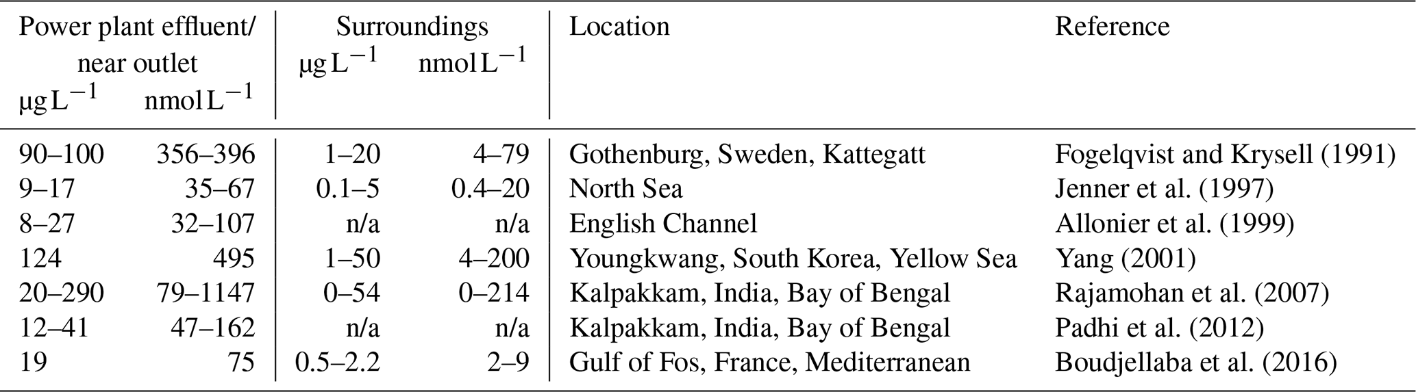
To determine the amount of bromoform produced in the cooling water, there are only a few measurements available and the locations are limited (Table 1). Most data originate from several power plants in Europe (Allonier et al., 1999; Boudjellaba et al., 2016; Jenner et al., 1997), and some studies are based on measurements from single power plants in Asia (Padhi et al., 2012; Rajamohan et al., 2007; Yang, 2001). Only Yang (2001) provides DBP measurements in East Asia. Furthermore, the location where water is sampled is not consistent among the different studies. Some samples were taken in the coastal surface water at the power plant outlet (Fogelqvist and Krysell, 1991; Yang, 2001), while other studies sampled directly inside the power plant before dilution with the ocean (Jenner et al., 1997; Rajamohan et al., 2007). The measurements show a very large variability ranging from 8–290 µg L−1. As there is no systematic difference between measurements inside the power plant and at the power plant outlet, both types of measurements are given in Table 1 together in the first column.
In addition to the sampling location, differences in the concentrations can result from water temperature, salinity and dissolved organic carbon content, which vary with season. Colder water from mid- to high latitudes during winter requires less water treatment as the growth of pathogens takes longer compared to warm tropical or subtropical waters. The chlorination dosage and frequency of treatment also play a distinct role for the resulting DBP concentrations (Joint Research Council, 2001).
Given that available measurements are sparse and depend on many factors, the uncertainties in initial bromoform concentrations in cooling water are relatively high. For our analyses we chose to scale the bromoform discharge according to three scenarios (LOW, MODERATE and HIGH), which reflect the range of values given in available literature (Table 1). For our simulations, we use initial bromoform concentrations of 20 µg L−1 (LOW), 60 µg L−1 (MODERATE) and 100 µg L−1 (HIGH) in undiluted cooling water.
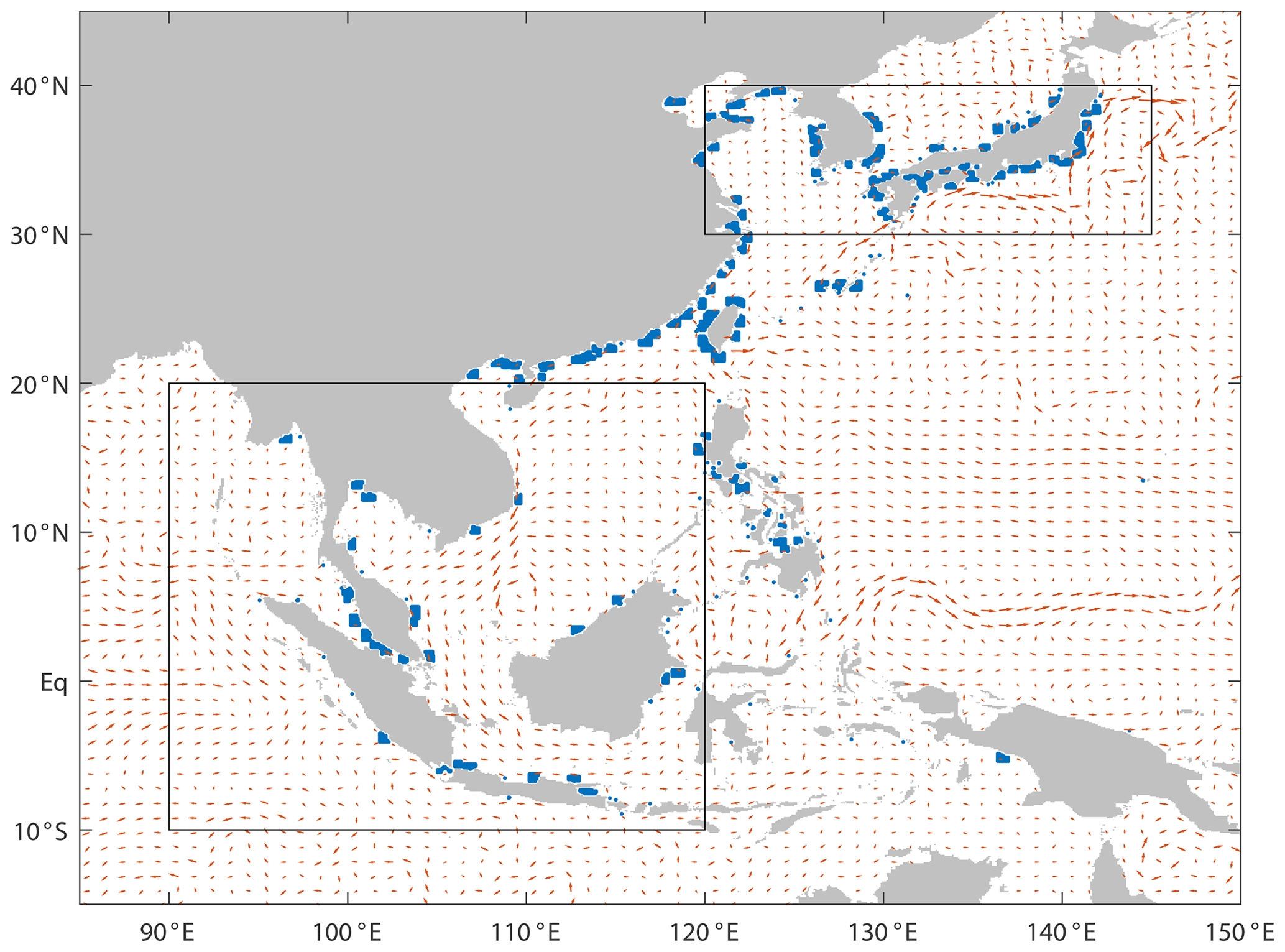
Figure 2Initial position of particles in East and Southeast Asia (blue dots). NEMO-ORCA0083 ocean currents from the initialisation time in January 2005 (red arrows); the two boxes mark the regions referred to as tropics and subtropics as described in Sect. 2.3.
2.2 Lagrangian simulations in the ocean
To assess the long-term, large-scale effect of DBPs from power plant cooling water on the environment, we simulate the distribution of non-volatile DBPs and the concentration and emission of the volatile DBP bromoform in the ocean. The Lagrangian model runs are based on velocity output from the high-resolution, eddy-rich ocean general circulation model (OGCM) NEMO-ORCA version 3.6 (Madec, 2008). The ORCA0083 configuration (The DRAKKAR Group, 2007) has a horizontal resolution of ∘ at 75 vertical levels, and output is given at a temporal resolution of 5 d for the time period 1963–2012. Atmospheric forcing comes from the DFS5.2 data set (Dussin et al., 2016). The experiment ORCA0083-N06 used in this study was run by the National Oceanography Centre, Southampton, UK. Further details can be found in Moat et al. (2016).
We simulate the spread of the DBPs from treated cooling water by applying a Lagrangian trajectory integration scheme to the 3D velocity fields with the Ariane software (Blanke et al., 1999). We perform offline trajectory calculations by passively advecting virtual particles, which represent the DBP amount discharged with the cooling water. The calculation of trajectories with Ariane is primarily based on advection. For each scenario we perform one simulation over the same time period from 2005/2006. The year chosen is the same as in Maas et al. (2019), where it is shown that interannual variability of surface velocity in the study region is small compared to seasonal variability. In each simulation, particles are continuously released close to the power plant locations at 5 d time steps over 2 years. We allow for an accumulation period of 11 months and show the results of the seasonal and annual mean of the second year starting in December 2005. A detailed description of the applied method can be found in Maas et al. (2019).
Our study focusses on the region of East and Southeast Asia (90–165∘ E, 10∘ S–45∘ N), which comprises 50 % of the global coastal power plant capacity and cooling-water discharge. The particle discharge locations have been chosen as close to the coastlines as possible (Fig. 2). Particles are released approximately 8 to 40 km offshore, as the model-resolution does not allow us to capture smaller-scale coastal structures such as harbours or estuaries, nor does it simulate the near-costal exchange, e.g. through tides. Our approach ensures minimal influence of the land boundaries on the simulation in order to avoid numerically related beaching of particles into the coastal boundary.
We conduct two different simulations allowing us to analyse the spread of long-lived DBPs in general and the spread of bromoform as a specific case. First, we simulate the spread of a passive tracer, which does not have any environmental sinks and is representative of long-lived non-volatile DBPs. We consider the full history of simulated particle positions which is equivalent to assuming no particles getting lost through sinks in the ocean or emission into the atmosphere. The resulting distribution shows locations where non-volatile DBPs such as bromoacetic acid are transported through the ocean currents within 1 year.
Second, we simulate the spread of bromoform as a major volatile DBP including the simulation of atmospheric fluxes and oceanic sinks. Each particle is assigned an initial mass of bromoform according to the amount of cooling water used by the respective power plant (Fig. 1) and the bromoform concentration prescribed by the three scenarios: MODERATE, HIGH and LOW. The particle density distribution is calculated at the sea surface down to 20 m on a grid. The distribution is given as particle density per grid box in percent for non-volatile DBPs and as concentration in pmol L−1 for bromoform.
For the second set of simulations, the sink processes of bromoform such as constant gas exchange at the air–sea interface or chemical loss rates are taken into account. The air–sea flux of bromoform is calculated following the general flux equation at the air–sea interface:
Here flux is positive when it is directed from the ocean to the atmosphere and is given in . Cw is the actual concentration in the surface mixed layer in pmol L−1, and
is the theoretical equilibrium concentration at the sea surface (in pmol L−1) calculated from the atmospheric mixing ratio (in ppt) and Henry's law constant of bromoform. The gas transfer velocity k (in cm h−1) mainly depends on the surface wind speed and temperature and is calculated following Nightingale et al. (2000). Wind velocities at 10 m height are taken from the NEMO-ORCA forcing data set DFS5.2 (Dussin et al., 2016), which is based on the ERA-Interim atmospheric data product.
As the oceanic and atmospheric terms in the air–sea flux parameterisation are of additive nature, it is possible to calculate the flux of anthropogenic and natural bromoform separately. For our simulations, we only consider bromoform from cooling water and apply the air–sea flux parameterisation to the anthropogenic portion of bromoform in water and air. We have conducted sensitivity tests (see Sect. 2.3) to estimate the impact that atmospheric bromoform abundances have upon the flux calculations. The tests show that outgassed anthropogenic bromoform leads to atmospheric surface values Ceq, which are always below 8 % of the underlying sea surface concentration Cw (at a water temperature of 20 ∘C). Such low equilibrium concentrations can be considered negligible for the flux calculation, and therefore Ceq is set to zero in our study.
The sea surface concentration and air–sea flux from the three simulations are also compared to climatological maps of bromoform concentration and emissions from the updated Ziska et al. (2013) inventory (hereafter referred to as Ziska2013) (Fiehn et al., 2018a).
Mean sea surface concentrations Cw are calculated by averaging over the area where 90 % of all released bromoform accumulates. To this end, all grid cells are sorted according to descending bromoform concentrations and the average is calculated over the first grid cells that contain in total 90 % of all bromoform. Maximum concentrations are calculated by averaging over the area where 10 % of the highest bromoform values accumulate. Mean and maximum air–sea fluxes are calculated using the same averaging principle as for Cw. The annual mean atmospheric bromine flux resulting from industrial bromoform emissions in East and Southeast Asia is derived from the air–sea flux maps of the whole domain.
2.3 Lagrangian simulation in the atmosphere
Based on the seasonal mean emission maps, we obtain a source function of atmospheric bromoform. We simulate the atmospheric transport and distribution of bromoform for the three different emission strength scenarios with the Lagrangian particle dispersion model FLEXPART (Stohl et al., 2005). The FLEXPART model includes parameterisation for moist convection (Forster et al., 2007) and turbulence in the boundary layer and free troposphere (Stohl and Thomson, 1999). It has been used in previous studies with a similar model set-up and shown robust VSLS profiles compared to observations (e.g. Fiehn et al., 2017; Fuhlbrügge et al., 2016; Tegtmeier et al., 2020a).
Seasonal mean bromoform emissions derived from the three scenarios are used as input data at the air–sea interface over the East and Southeast Asia area defined as our study region. The meteorological input data (temperature and winds) stem from the ERA-Interim reanalysis product (Dee et al., 2011) and are given on a horizontal grid, at 61 vertical model levels and a 3-hourly temporal resolution. The chemical decay of bromoform in the atmosphere was accounted for by prescribing a lifetime of 17 d during all runs (Montzka and Reimann, 2010).
The FLEXPART simulations were performed for boreal winter (December–February, DJF) and summer (June–August, JJA) seasons, respectively, each with a 2-month spin-up phase. Since there are only weak dynamical variations between different years, we used an ensemble mean of 4 years (2015–2018) each. A total of 1000 particles are randomly seeded inside each grid box at each time step according to the air–sea flux strength. Output mixing ratios are given at the same horizontal resolution and 33 vertical levels from 50 to 20 000 m. Detailed descriptions of model settings are described in Jia et al. (2019).
We perform three additional FLEXPART runs, Ziska2013-EastAsia, Ziska2013 and Ziska2013 + MODERATE, based on the updated Ziska2013 emission inventory with the same FLEXPART configuration as described above for both seasons, DJF and JJA. As the Ziska2013 inventory currently presents our best knowledge of bottom-up bromoform emissions, it is of interest to analyse how much of these emissions can be explained by industrial sources and how much stems from natural sources.
The Ziska2013-EastAsia run uses only the Ziska2013 climatological emissions over East and Southeast Asia defined as our study region. Results from Ziska2013-EastAsia in the atmospheric boundary layer are used to compare the mixing ratios based on our anthropogenic emissions in the East and Southeast Asia region.
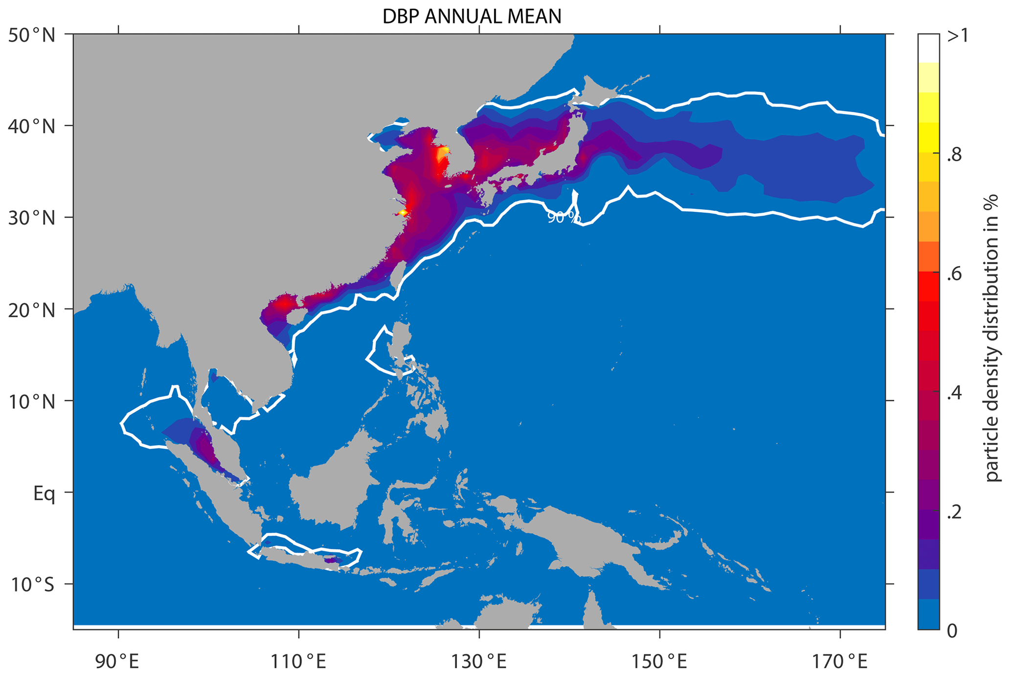
Figure 3Annual mean particle density distribution in percent (%) of DBPs from cooling-water treatment in coastal power plants in East and Southeast Asia. The white contour line shows the patches where 90 % of the largest particle density is located.
For comparisons of mixing ratios in the free troposphere and upper troposphere–lower stratosphere (UTLS), air–sea fluxes from other parts of the tropics also need to be taken into account as the timescales for horizontal transport are often shorter than the ones for vertical transport. Therefore, we set up the runs Ziska2013 and Ziska2013 + MODERATE. Ziska2013 uses the air–sea flux of the Ziska2013 climatology for the global tropics and subtropics between 45∘ S and 45∘ N. As the Ziska2013 climatology is taking into account only very few northern hemispheric coastal data points, it likely neglects anthropogenic fluxes in some regions. Therefore, the Ziska2013 + MODERATE run uses the Ziska2013 fluxes between 45∘ S and 45∘ N but replaces them with the anthropogenic MODERATE flux values in all grid boxes where the MODERATE fluxes are larger than the Ziska2013 fluxes. The two runs, Ziska2013 + MODERATE and Ziska2013, are used to quantify the additional anthropogenic bromoform based on the MODERATE scenario in the UTLS region. The UTLS region is calculated as the height of the cold-point tropopause, which has been derived from ERA-Interim model level data at 6-hourly resolution (Tegtmeier et al., 2020b).
Mean mixing ratios from the whole domain (90–165∘ E, 10∘ S–45∘ N) in the marine boundary layer and in the UTLS are given as the average over the 90 % area characterised by the highest local values, and maximum mixing ratios are given as the average over the largest 10 % (see Sect. 2.2). In a second step, we define two regions in order to analyse the vertical transport of bromoform into the free troposphere and into the UTLS. For the height profiles of the Ziska2013 and the Ziska2013 + MODERATE runs, we average mixing ratios over a region above the Maritime Continent, which we refer to as the tropical box (10∘ S–20∘ N, 90–120∘ E), and over another region from China to Japan, which we refer to as the subtropical box (30–40∘ N, 120–145∘ E) (Fig. 2).
The particle density distribution shows the annual mean DBP accumulation pattern in the region of interest in East and Southeast Asia (Fig. 3). Non-volatile DBPs from cooling water usually accumulate around the coast and in the marginal seas. There is a clear latitudinal gradient with only little DBP distribution south of 20∘ N, except for higher values in the Strait of Malacca. In contrast to the relatively low DBP density in the inner tropics, the subtropics show a very high accumulation of DBPs with a centre in the marginal seas between 25 and 40∘ N. While power plants can be found along all coastlines (Fig. 1), the power plant capacity and therefore the amount of treated cooling water is much higher along the subtropical coasts of China, Korea and Japan, leading to the DBP distribution pattern shown in Fig. 3. Hotspots are around the coast of Shanghai and Incheon, with a DBP density of 1 %. A relatively high DBP density of 0.8 % can also be found in the East China Sea, the Yellow Sea, the southern Sea of Japan, the Gulf of Tonkin and the Strait of Malacca. Medium to low DBP density in the South China Sea suggests only small contributions of cooling waters to this region. Since Japan and Korea have a large number of power plants with high volumes of cooling-water discharge, a relatively large amount of DBPs is transported eastward with the Kuroshio Current east of Japan into the North Pacific.
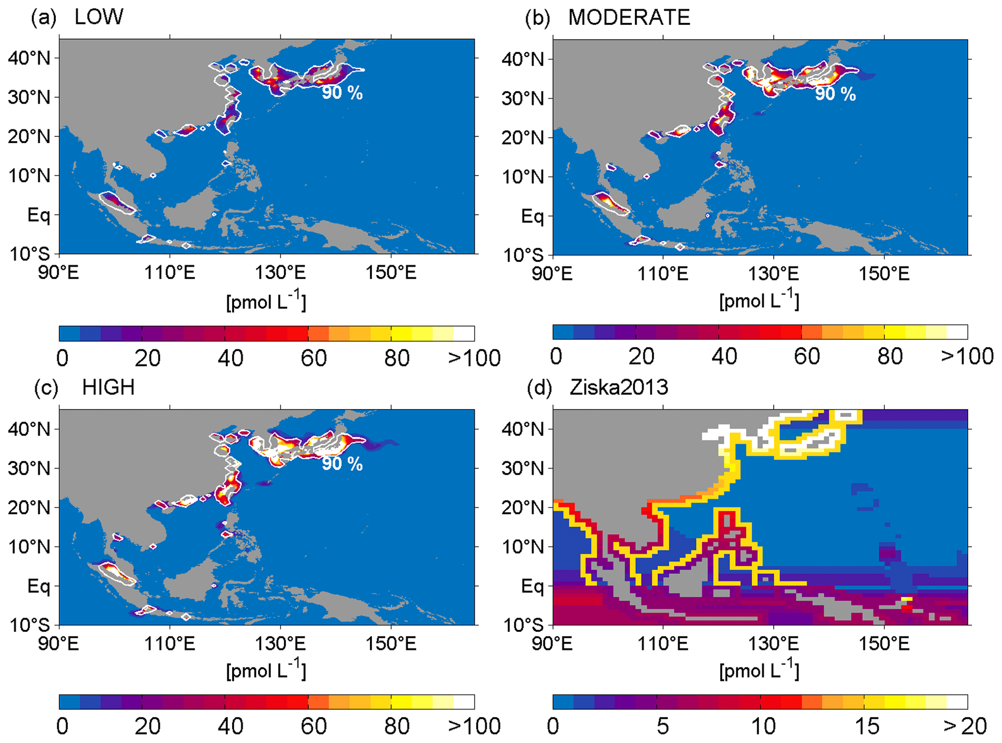
Figure 4Annual mean surface bromoform concentration in pmol L−1 for the three scenarios (a) LOW, (b) MODERATE and (c) HIGH as well as (d) the bromoform surface map updated from Ziska2013. Note that the colour bar limits for panel (d) vary from the limits in panels (a)–(c). The white contour line in panels (a)–(c) shows the patches where 90 % of the largest concentrations are located.
The distribution of bromoform as a volatile DBP in the surface ocean differs from the DBP accumulation pattern shown in Fig. 3, because the volatile DBPs are outgassed into the atmosphere. The annual mean sea surface concentration of bromoform from cooling water is shown in Fig. 4a–c for the three cooling-water discharge scenarios LOW, MODERATE and HIGH and with a substantially smaller spread compared to the non-volatile DBPs. The area which contains the 90 % highest bromoform concentrations does not vary between the three scenarios, as the air–sea flux, which determines how much bromoform remains in the water, is linearly proportional to the sea surface concentration. Higher surface concentrations result in higher fluxes into the atmosphere, which limits the spread of bromoform substantially compared to non-volatile DBPs. Bromoform concentrations are around 23, 68 and 113 pmol L−1 (LOW, MODERATE and HIGH), averaged over the region where the 90 % of bromoform with the highest concentrations accumulates (Table 2). This region is to a large degree limited to latitudes north of 20∘ N as a result of the power plant distribution. As in the case of the non-volatile DBPs, most of the bromoform is centred along the Chinese, Korean and Japanese coastline, with a larger spread into the marginal seas for the latter two. One exception to this latitudinal gradient is the Strait of Malacca, where local power plants result in average bromoform concentrations of 3.4, 10.3 and 16.7 pmol L−1 (LOW, MODERATE, and HIGH).
Table 2Mean and maximum bromoform concentration [pmol L−1] for the three Ariane runs LOW, MODERATE, and HIGH, as well as the climatological values from the Ziska2013 bottom-up estimate in East and Southeast Asia. Mean and maximum air–sea flux [] from the three scenarios and the Ziska2013 air–sea flux in East and Southeast Asia. The annual mean bromine flux [Mmol Br a−1] is derived from the air–sea flux of the total domain in East and Southeast Asia. Mean and maximum atmospheric bromoform mixing ratios in the marine boundary layer [ppt] from the four FLEXPART runs. Values are given as the mean and the standard deviation averaged over the largest 90 % (referred to as mean values) and over the largest 10 % (referred to as maximum values).
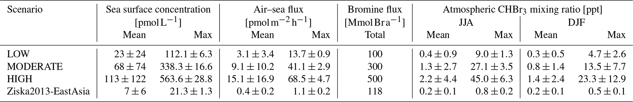
Observation-based oceanic bromoform concentrations from Ziska2013 (Fig. 4d) are relatively evenly spread along the coastlines of the region and do not show the latitudinal gradient found for the anthropogenic concentrations. North of 20∘ N the anthropogenic bromoform is much higher than the oceanic distribution from Ziska2013, where the maximum lies around 21 pmol L−1. Our simulations reach maximum values (averaged over the 10 % highest bromoform concentrations) of 112, 338 and up to 563 pmol L−1 (LOW, MODERATE and HIGH, Table 2) in the Sea of Japan. These concentrations are all above 100 pmol L−1 and are very high compared to observational values from Ziska2013 (Fig. 4d).
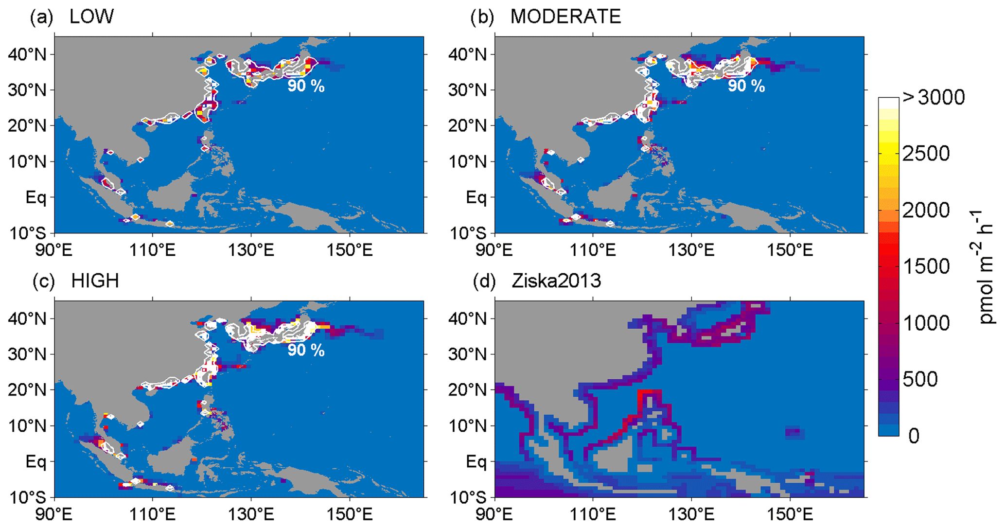
Figure 5Annual mean air–sea flux of bromoform in for the three scenarios (a) LOW, (b) MODERATE, and (c) HIGH, as well as (d) the air–sea flux calculated from updated ocean and atmospheric maps following Ziska2013. The white contour line in panels (a)–(c) shows the patches where 90 % of the largest emissions are located.
Air–sea fluxes of anthropogenic bromoform show a similar distribution as the oceanic concentrations (Fig. 5a–c). Flux rates averaged over the region of the 90 % highest flux values are 3, 9 and 15 (LOW, MODERATE and HIGH). Maximum flux rates (averaged over the highest 10 %) even reach 13, 41 and 68 in the Sea of Japan near the Korean and Japanese coast for the three scenarios (Table 2). In contrast, the existing observation-based estimates from the Ziska2013 climatology peak with a flux of 1.1 in the South China Sea along the west coast of the Philippines (Fig. 5d).
The annual bromine input from the ocean into the atmosphere in the form of bromoform emissions in the East and Southeast Asia region is 118 Mmol of Br according to the observation-based inventories from Ziska2013 (Table 2). Our simulations suggest that the anthropogenic input alone amounts to 100, 300 and 500 Mmol Br a−1 (LOW, MODERATE and HIGH) for the same region, which corresponds to almost 99 % of the bromine produced during cooling-water treatment in the power plant for each scenario. This implies that all bromoform from cooling-water treatment is eventually outgassed from the ocean into the atmosphere. While average and maximum air–sea fluxes of anthropogenic bromoform are much higher and confined to small areas around the discharge locations, the Ziska2013 air–sea fluxes are distributed along all coastlines and along the Equator and result in a similar total annual mean Br flux as the LOW emission scenario (Table 2). A total of 90 % of the annual mean atmospheric bromine input from anthropogenic bromoform in East Asia occurs north of 20∘ N where 89–447 Mmol of Br is released over 1 year, compared to the tropical Southeast Asian regions south of 20∘ N where only 10–52 Mmol Br a−1 enters the atmosphere (from LOW to HIGH). In contrast, only 29 % of the total bromine from the Ziska2013 climatology in East Asia is released into the atmosphere north of 20∘ N, which suggests that the majority of the anthropogenic emissions from this region are missing in the Ziska2013 climatology.

Figure 6Seasonal mean bromoform mixing ratios [ppt] in 50 m height during JJA derived from FLEXPART runs driven by the three scenarios (a) LOW, (b) MODERATE, (c) HIGH, and (d) Ziska2013-EastAsia.
4.1 Mixing ratios in the marine boundary layer
Atmospheric mixing ratios of anthropogenic bromoform are derived from FLEXPART runs driven by the seasonal emission estimates discussed in Sect. 3. Atmospheric bromoform from industrial emissions is shown for a seasonal average in the marine boundary layer at 50 m height for JJA for all three scenarios (Fig. 6a–c). Mean mixing ratios are 0.4, 1.3 and 2.3 ppt (LOW, MODERATE and HIGH, Table 2). Overall, high atmospheric mixing ratios are found around the coastlines of Japan, South Korea and northern China. Although maximum emissions are located in the Sea of Japan, maximum mixing ratios are mostly located south of Japan with values up to 9.0, 27.1 and 45.0 ppt (LOW, MODERATE and HIGH, Table 2). Here, the westerlies lead to bromoform transport from the Sea of Japan into the northwest Pacific. We also localise hotspots of strong anthropogenic bromoform accumulations due to enhanced emissions over Shanghai, Singapore or the Pearl River Delta, respectively (Fig. 6a). During boreal summer, the western Pacific and Maritime Continent are influenced by southwesterly winds, and the anthropogenic bromoform experiences northward transport, bringing some smaller portion of the subtropical emissions into the mid-latitudes (Fig. 6a–c).

Figure 7Same as Fig. 6 only during DJF.
During boreal winter (DJF, Fig. 7a–c), anthropogenic bromoform shows somewhat lower atmospheric mixing ratios with a mean of 0.3, 0.8 and 1.4 ppt and maximum values of 4.7, 13.5 and 23.3 ppt for the three scenarios (Table 2). In contrast to boreal summer, the atmospheric transport is dominated by winds from the northeast, and higher bromoform values are confined to tropical and subtropical regions (Fig. 7). Thus, tropical mixing ratios show a clear seasonal variability and are on average over 3 times higher for DJF than for JJA without large shifts in the location of the bromoform emissions (Fig. S1 in the Supplement).
In order to compare the atmospheric impact of industrial emissions with existing results, we repeat our analysis for the bottom-up emissions scenario Ziska2013 for the same region, which has been frequently used in past studies (e.g. Hossaini et al., 2013, 2016). Atmospheric mixing ratios are derived from seasonal FLEXPART runs driven by Ziska2013-EastAsia and shown for a seasonal average at 50 m height for JJA (Fig. 6d). For both seasons, JJA and DJF, atmospheric bromoform based on industrial emissions is larger than atmospheric bromoform based on the Ziska2013-EastAsia emissions (Figs. 6d and 7d). These differences are maximised in the subtropical regions, where anthropogenic bromoform dominates especially during JJA when anthropogenic mixing ratios are 2–5 times larger compared to climatological Ziska2013 bromoform (for LOW and MODERATE). In the tropical regions, the situation is more complicated. Atmospheric abundances driven by the industrial emissions reach higher peak values of up to 2 ppt, especially in the Strait of Malacca (MODERATE, Fig. 6b), while mixing ratios driven by the observationally based emissions from Ziska2013-EastAsia are smaller, only reaching peak values of up to 0.8 ppt, but are spread over a much wider area (Fig. 6d). Given the comparison of the boundary layer values, it is not clear which emission scenario will result in a larger contribution to the stratospheric halogen budget.
4.2 Mixing ratios in the free troposphere and UTLS
In order to analyse atmospheric transport from the marine boundary layer into the free troposphere and UTLS, seasonal mean bromoform mixing rations are averaged over a subtropical box (30–40∘ N, 120–145∘ E, Fig. 2) and a tropical box (10∘ S–20∘ N, 90–120∘ E, Fig. 2) from the Ziska2013 and Ziska2013 + MODERATE simulations for DJF and JJA. Both simulations are based on global climatological Ziska2013 bromoform air–sea fluxes between 45∘ S and 45∘ N, with Ziska2013 + MODERATE including additional anthropogenic bromoform fluxes in East and Southeast Asia.
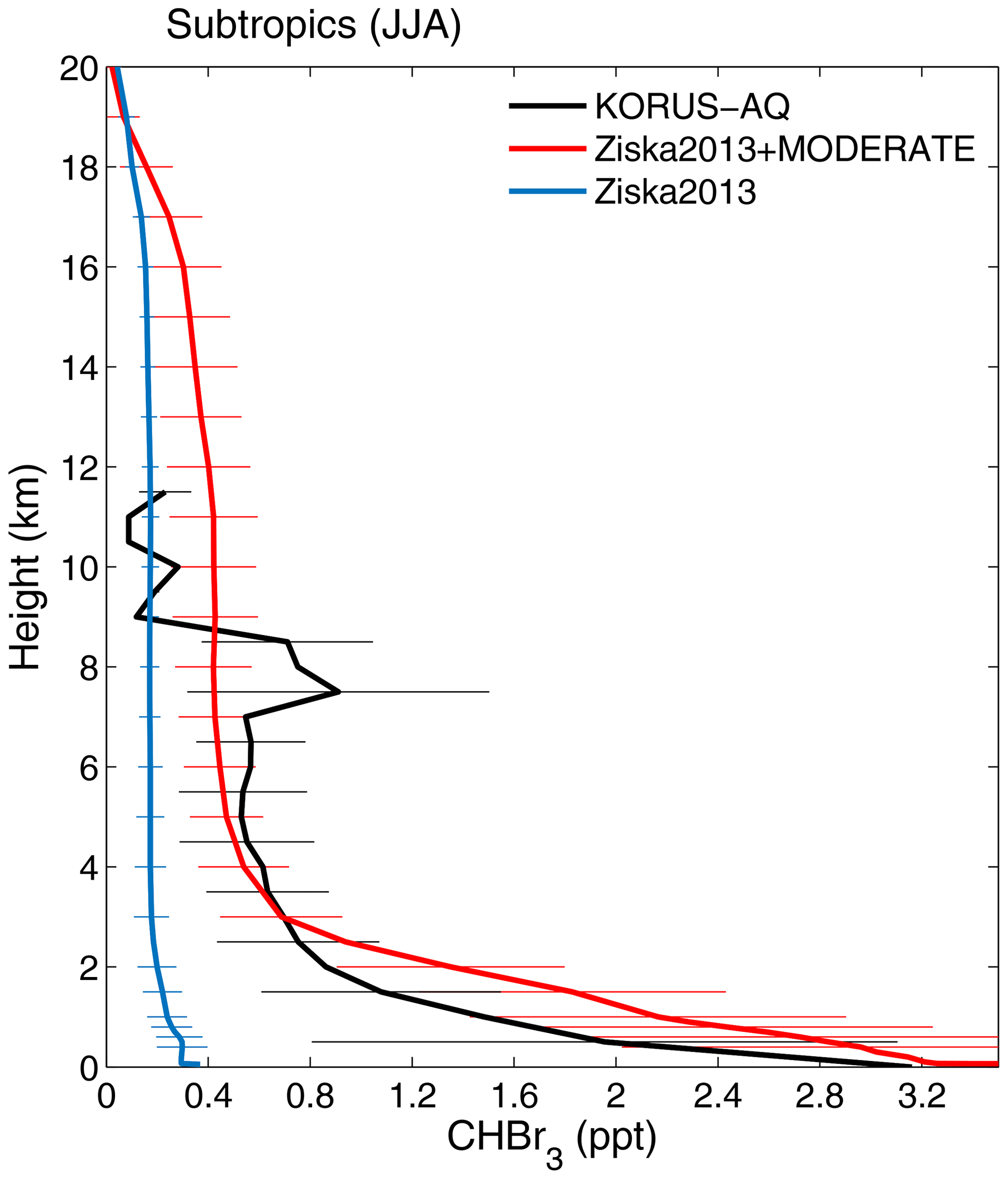
Figure 8Height profile of seasonal mean bromoform mixing ratio [ppt] in the subtropics (30–40∘ N, 120–145∘ E) during JJA for the Ziska2013 + MODERATE run (red) and the Ziska2013 run (blue). Additionally shown is the averaged profile of bromoform measurements from the KORUS-AQ campaign over South Korea and the Yellow Sea (black). Horizontal lines show the standard deviation for specific heights.
In the subtropical box (Fig. 8), there is a strong dominance of anthropogenic bromoform in the marine boundary layer during JJA that is several times higher compared to bromoform from climatological bottom-up emissions (Fig. 8). Our simulations suggest that during convective events in JJA, anthropogenic bromoform from the subtropical marine boundary layer can be transported into the UTLS region, up to the height of the cold point. In our simulation Ziska2013 + MODERATE, convective events during the summer bring on average over 0.3 ppt into the UTLS (Fig. 8). During DJF (not shown), there is only very little transport of bromoform out of the boundary layer, and entrainment of anthropogenic bromoform into the subtropical UTLS is confined to boreal summer when the Intertropical Convergence Zone (ITCZ) is located north of 10∘ N (Waliser and Gautier, 1993).
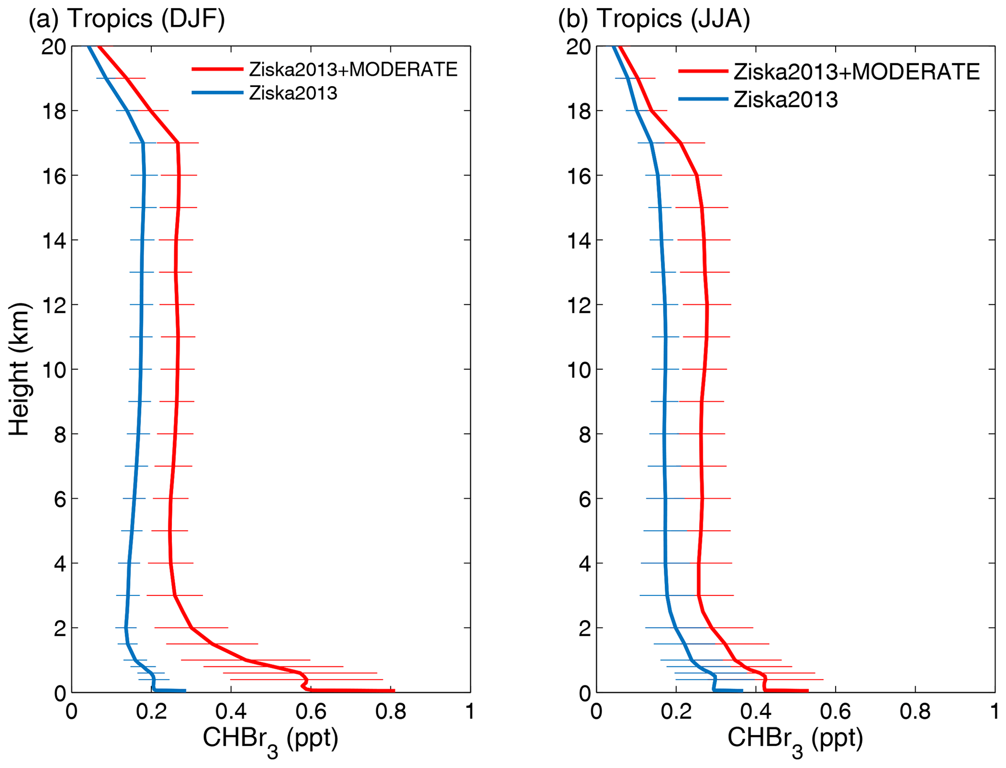
Figure 9Height profile of seasonal mean bromoform mixing ratio [ppt] in the tropics (10∘ S–20∘ N, 90–120∘ E) for the Ziska2013 + MODERATE run (red) and Ziska2013 run (blue) for both (a) DJF and (b) JJA. Horizontal lines show the standard deviation for specific heights.
In the tropical box (Fig. 9), atmospheric bromoform mixing ratios in the marine boundary layer are generally weaker than in the subtropics (Fig. 8). The seasonal difference between DJF and JJA is only pronounced in the tropical marine boundary layer for Ziska2013 + MODERATE, where mixing ratios during DJF exceed 0.5 ppt throughout the whole time period (Fig. 9a) and are around 0.4 ppt during JJA (Fig. 9b). The air–sea fluxes show no strong seasonal variations; therefore, this difference must be transport driven. During DJF, the prevailing northeasterly winds advect the bromoform from regions of high anthropogenic emissions in East Asia towards the Maritime Continent, increasing the tropical bromoform abundance substantially. Thus, tropical convection during DJF can transport more of the anthropogenic bromoform emitted in East Asia into the UTLS compared to similar events during JJA (Fig. 9). The difference between the Ziska2013 + MODERATE and the Ziska2013 average mixing ratios in the UTLS is 0.05 ppt during DJF and 0.04 ppt during JJA. These values present the anthropogenic contribution to stratospheric bromine from East and Southeast Asian cooling water based on the MODERATE bromoform emission scenario.
Atmospheric processes over the Maritime Continent, which encloses the tropical box, are characterised by deep convective events, which can lead to entrainment of VSLSs into the stratosphere (Aschmann and Sinnhuber, 2013; Tegtmeier et al., 2020a). For our case study, convective events reaching the UTLS occur in both seasons (Fig. 9). Moreover, here is a clear anthropogenic signal from Ziska2013 + MODERATE compared to Ziska2013 in the free troposphere in this region in both seasons, which is more pronounced during DJF (Fig. 9a) than during JJA (Fig. 9b), in agreement with the elevated mixing ratios in the marine boundary layer.

Figure 10Seasonal mean atmospheric CHBr3 mixing ratios [ppt] for (a, b) the Ziska2013 + MODERATE and (c, d) the Ziska2013 simulation at the cold-point tropopause height for (a, c) DJF and (b, d) JJA.
In addition to the mixing ratios averaged over two boxes, we show the spatial distribution of seasonally averaged bromoform mixing ratios at the cold-point tropopause for the whole domain (90–165∘ E, 10∘ S–45∘ N) (Fig. 10) based on the Ziska2013 and Ziska2013 + MODERATE emissions. During DJF (Fig. 10a and c), there is a clear anthropogenic signal over the Bay of Bengal, across the Equator towards Indonesia. Mixing ratios for the Ziska2013 + MODERATE run are 0.22±0.07 ppt, averaged over the area of 90 % highest mixing ratios, and 0.18±0.05 ppt for Ziska2013, which implies that 0.04 ppt is of anthropogenic origin (Table S1 in the Supplement). Again, the strong advective transport in the boundary layer during DJF bringing higher bromoform abundances from the subtropics into the tropics plays an important role here. Some fraction of the advected bromoform is picked up by tropical deep convection and transported into the UTLS and up to the cold point. As the latter represents the stratospheric injection level, the interaction of boundary layer advection and local convection over the Indian Ocean and Maritime Continent results in an efficient transport pathway for anthropogenic bromoform from industrial sources in East Asia to the stratosphere.
During JJA (Fig. 10b and d), mean bromoform mixing ratios averaged over the area of 90 % highest mixing ratios are slightly smaller, with 0.20±0.06 and 0.15±0.05 ppt based on the Ziska2013 + MODERATE and Ziska2013 emissions, respectively (Table S1). During the Asian summer monsoon, the region of main upward transport of VSLS lies at about 20∘ N over the Indian Ocean so that the main stratospheric injection region of VSLSs shifts to the Bay of Bengal and northern India (Fiehn et al., 2018b). However, most of the boundary layer bromoform from anthropogenic sources stays in the Northern Hemisphere around the coastline of China and over the western Pacific, thus decoupled from the monsoon convection.
While over 90 % of anthropogenic bromoform is outgassed north of 20∘ N, our simulations show that the additional anthropogenic emissions in the MODERATE scenario contribute on average 0.05 ppt of CHBr3 during JJA to 0.04 ppt of CHBr3 during DJF to the stratospheric bromine budget at the UTLS (Table S1). This is an increase of 22 %–32 % compared to the Ziska2013 mixing ratios of 0.15 and 0.18 ppt of CHBr3 during JJA and DJF, respectively.
5.1 Comparison with bromoform measurements in the ocean
Observations of bromoform in the surface ocean and atmosphere from East and Southeast Asia can help to determine which scenario (LOW, MODERATE and HIGH) offers the best fit for simulating anthropogenic bromoform in this region. Recent measurement campaigns show elevated bromoform concentrations in the coastal waters of the East China and Yellow seas (He et al., 2013a, b; Yang et al., 2014, 2015). Average values of 6–13 pmol L−1 were measured in the Yellow and East China seas during boreal spring and summer (Yang et al., 2014, 2015), and 17 pmol L−1 was measured in boreal winter (He et al., 2013b). Particularly high concentrations were detected by He et al. (2013a) during spring in the East China Sea with a mean of 134 pmol L−1. The highest bromoform concentration over 34 pmol L−1 (He et al., 2013b) and over 200 pmol L−1 (He et al., 2013a) was observed near the estuaries of the Yangtze River, which the authors attributed to anthropogenic activities including coastal water treatment in the Shanghai region. Our simulations also show mean surface concentrations around Shanghai of 14–71 pmol L−1 (LOW to HIGH), in the range of the observations by He et al. (2013a).
Measurements in the South China and Sulu seas (Fuhlbrügge et al., 2016) show a high variability of bromoform in the surface seawater with average concentrations of 19.9 pmol L−1. The highest values of up to 136.9 pmol L−1 are found close to the Malaysian Peninsula and especially in the Singapore Strait, suggesting industrial contributions. Maximum anthropogenic bromoform from our simulations in the Singapore Strait ranges from 36–178 pmol L−1 (LOW to HIGH), in good agreement with maximum values reported by Fuhlbrügge et al. (2016).
Average anthropogenic bromoform concentrations for the three scenarios are around 23–113 pmol L−1 (averaged over the region of the 90 % highest values, Table 2) and are larger than the observational average values. The larger model values might be due to the fact that the cooling-water effluents do not distribute far into the marginal seas but stay near the coast as observed by Yang (2001) and confirmed by our simulations. Our simulated anthropogenic bromoform concentrations stay usually within 100 km of the coast; the averaged observational values, however, include also measurements that are up to 200 km away from the coastline and can therefore be expected to be lower. While observational mean values are slightly lower than our model results, maximum values found close to the coastline show very good agreement with the model results.
5.2 Comparison with bromoform measurements in the troposphere
An extensive study of atmospheric measurements over South Korea and adjacent seas was performed in spring (May and June) 2016 by the Korea–United Sates Air Quality Study (KORUS-AQ; https://www-air.larc.nasa.gov/missions/korus-aq/, last access: 1 March 2021). The aircraft measurements of various VSLSs including bromoform were repeatedly taken between 0 and 12 km in the region between 30–40∘ N and 120–145∘ E, coinciding with our subtropical box discussed earlier (Fig. S2). The data used here are based on the 60 s merged data set from all flight sections. In the campaign region around South Korea, an average bromoform atmospheric mixing ratio from all sections of 2.5±1.4 ppt was measured in the lower 100 m (Fig. 8). In comparison, our simulations for the Ziska2013 + MODERATE scenario show an average mixing ratio of 3.8±1.4 ppt in the lowest 100 m in the subtropical box during JJA. The simulations based on Ziska2013 give a bromoform mixing ratio of only 0.3±0.1 ppt for the same altitude range, demonstrating that the additional anthropogenic bromoform results in a much better agreement with the observations in the marine boundary layer around South Korea.
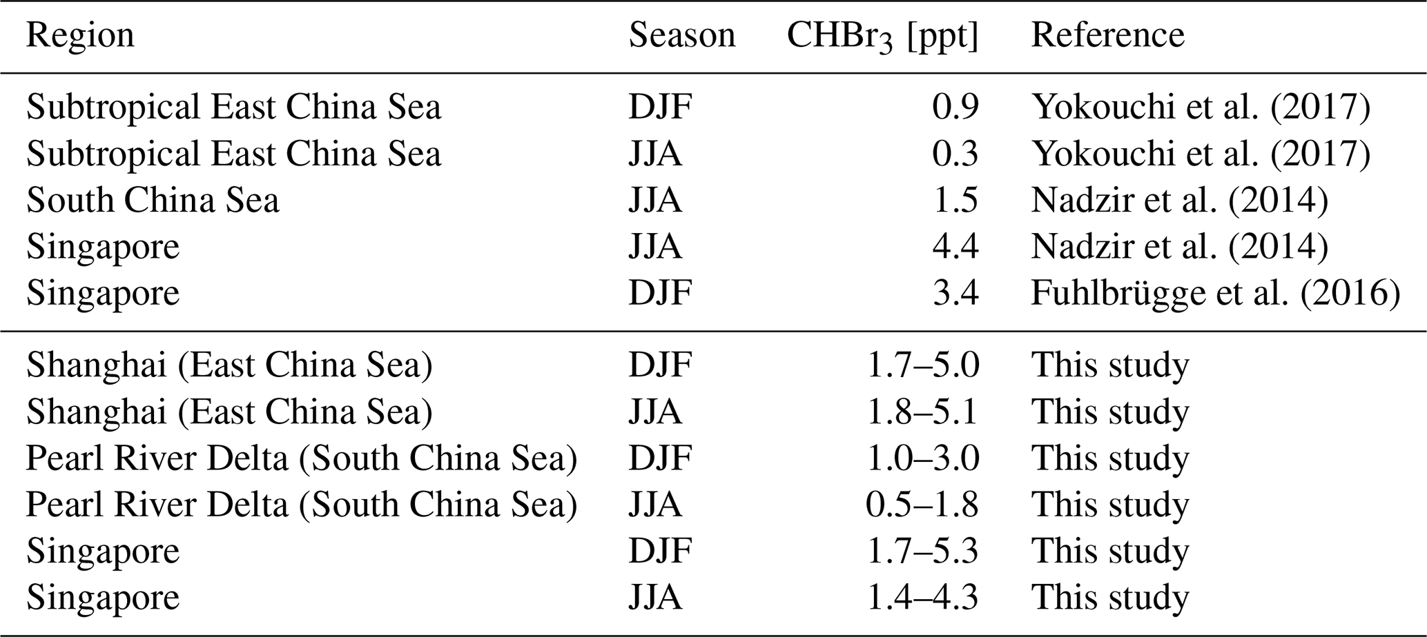
Table 3Observations with reference and corresponding range of mean modelled bromoform mixing ratios [ppt] from the FLEXPART simulations LOW and MODERATE from this study.
Above the boundary layer, mixing ratios from KORUS-AQ rapidly decline to 0.5–0.7 ppt in the 3–9 km altitude range (Fig. 8). Here, the Ziska2013 + MODERATE simulation suggest seasonal mean mixing ratios between 0.4–0.7 ppt, which fit very well to the KORUS-AQ data. Simulations based on Ziska2013 suggest 0.2 ppt bromoform in this region, clearly underestimating the observations (Fig. 8). Between 9 and 12 km, the observed bromoform values drop sharply to values around 0.2±0.08 ppt, suggesting that the aeroplane probed air masses above the convective outflow. The smooth seasonal mean profiles from the two simulations do not show such a sharp decrease in values, and in consequence the lower Ziska2013 results agree better with the observations in the height 9–12 km. In general, the comparison with the KORUS-AQ data shows that our simulations agree quite well with the observations in the middle troposphere when anthropogenic emissions from cooling-water treatment in East Asia are included based on the MODERATE scenario.
Additional bromoform mixing ratios from observations near large industrial cities are shown in Table 3. In the subtropical East China Sea, surface measurements are available and atmospheric mixing ratios of 0.9 and 0.3 ppt were found during boreal winter and summer, respectively (Yokouchi et al., 2017). Our simulations in the East China Sea suggest anthropogenic bromoform contributions of 1.7–5.1 ppt near Shanghai, being on the upper side of the observations (Table 3). Nadzir et al. (2014) observed relatively high values in the South China Sea (1.5 ppt) during boreal summer. Our simulations show average mixing ratios of 0.5–1.8 ppt at the surface (LOW to MODERATE) near the Pearl River Delta in the South China Sea, in good agreement with Nadzir et al. (2014) (Table 3). Around Singapore, high oceanic bromoform concentrations were measured to be 4.4 ppt during JJA (Nadzir et al., 2014) and 3.4 ppt during DJF (Fuhlbrügge et al., 2016). Our simulations result in peak bromoform mixing ratios near Singapore of 1.4–4.3 ppt for JJA and of 1.7–5.3 ppt for DJF (LOW and MODERATE), respectively, in good agreement with Nadzir et al. (2014) and Fuhlbrügge et al. (2016) (Table 3). Especially the high atmospheric bromoform mixing ratios found near Singapore and the Pearl River Delta can be associated with anthropogenic activity.
The HIGH scenario shows average mixing ratios, which are in general too high for the whole domain. Thus, it is not likely that cooling-water treatment produces anthropogenic bromoform with average concentrations of 100 µg L−1. Nevertheless, such concentrations can occur at some locations and produce extremely high bromoform abundances near the coast of industrial regions, as confirmed by the observations presented here.
5.3 Discussion of uncertainties
Our analyses suggests that anthropogenic bromoform accumulates in the boundary layer, increasing the bromine budget in East and Southeast Asia by 85 %–254 % compared to the Ziska2013 climatology. This input can be expected to impact tropospheric bromine budget and ozone chemistry. While we have not analysed these aspects in our study, it should be investigated in follow-on projects. The highest uncertainties in the estimates presented here arise from the highly variable bromoform amounts found in chemically treated cooling water. Since there are very few and no recent measurements from power plants in East and Southeast Asia available, the chosen scenarios aim to give a range of environmental concentrations of anthropogenic bromoform. Additional uncertainties can arise from oceanic and atmospheric transport simulations and the parameterisation of air–sea fluxes. Since bromoform is emitted into the atmosphere on very short timescales, uncertainties arising from oceanic transport simulations are small compared to scenario uncertainties. Similarly, given the high saturation of anthropogenic bromoform in surface water, the sensitivity of our results to the air–sea flux parameterisation can be expected to be small.
Atmospheric modelling can introduce additional uncertainties, especially regarding the contribution of anthropogenic sources to stratospheric bromine. VSLS FLEXPART simulations have been evaluated in numerous previous studies and shown in most cases to give good agreement with upper air observations (e.g. Fuhlbruegge et al., 2016; Tegtmeier et al., 2020a). In summary, uncertainties of our results are dominated by uncertainties of the bromoform concentrations in undiluted cooling water. We have successfully reduced these uncertainties by nearly a factor of 2 based on comparing our predictions to available observations.
5.4 Discussion of stratospheric entrainment
If bromoform is entrained into the stratosphere, it will contribute to ozone depletion driven by catalytic cycles. Atmospheric transport simulations show that during boreal winter strong northeasterly winds transport the anthropogenic bromoform from the East China Sea towards the tropics. Here, it can be taken up by deep convection and reach the cold-point tropopause, thus being entrained into the stratosphere. On average, 0.22 ppt of bromoform is entrained above the cold point based on natural and additional anthropogenic emissions (from the MODERATE scenario). For the same configuration during boreal summer, the large amount of anthropogenic bromoform emitted over the East China Sea does not reach the tropics, resulting in average mixing ratios of 0.20 ppt at the cold-point level. In summary, the high anthropogenic bromoform emissions in the East China Sea, Yellow Sea and Sea of Japan do not efficiently reach the stratosphere, except for some fraction that is advected with the Asian winter monsoon into the tropics, in which case it can lead to an increased entrainment of 22 %–32 % over this area when compared to Ziska2013. Comparison with measurements up to 12 km in the subtropics shows that the simulated bromoform agrees very well with the observations if additional anthropogenic sources from the MODERATE scenario are included. The good agreement suggests that anthropogenic bromoform can lead to an additional stratospheric entrainment of 0.04–0.05 ppt of CHBr3, which corresponds to a bromine input of 0.12–0.15 ppt of Br.
This study focusses on source gas entrainment into the stratosphere and does not take into account additional product gas entrainment resulting from anthropogenic bromoform sources. Most observational and modelling studies estimate the total stratospheric bromine contribution to be split half and half into source and product gas contributions (Engel and Rigby, 2018, and references therein). Therefore, we estimate the total stratospheric bromine contribution in the form of both source gas and product gases from the East and Southeast Asia anthropogenic bromoform sources to be around 0.24–0.30 ppt of Br. Compared to a total stratospheric bromine contribution from all VSLSs of about 3–7 ppt of Br (Engel and Rigby, 2018), the anthropogenic input estimated in this study provides only a minor contribution.
We predict that there is a strong anthropogenic source of bromoform along the coast of East Asia, with particularly large contributions north of 20∘ N from the East China Sea, Yellow Sea and Sea of Japan. This anthropogenic source results from local cooling-water treatment in power plants and leads to extremely high annual mean air–sea flux rates of 3.1–9.1 in coastal waters in East Asia. Simulations of atmospheric bromoform originating from industrial sources show an accumulation in the marine boundary layer and result in mean bromoform mixing ratios of 0.4–1.3 ppt. The simulations show a strong seasonal variability with high bromoform abundances being transported into the mid-latitudes during boreal summer and into the tropics during boreal winter. In comparison, the bottom-up inventory by Ziska2013 shows much lower concentrations along the coast of East Asia but higher mean sea surface concentrations in Southeast Asia. Our predictions are based on assuming initial bromoform concentrations in chemically treated cooling water from power plants. These concentrations depend on many different factors, and observational studies provide a range of 8–290 µg CHBr3 L−1. We take the large range of possible bromoform concentrations into account by analysing three different scenarios that assume LOW, MODERATE and HIGH bromoform concentrations in undiluted cooling water.
We evaluate our predictions by comparing the model results to available measurement data in the ocean and atmosphere. Comparisons with some individual campaigns suggest that our averaged anthropogenic values based on the MODERATE scenario agree very well with the observations. For other campaigns, the model results overestimate campaign-averaged bromoform concentrations in surface water and air. The latter discrepancy of the mean values is possibly related to the regional extent of the specific campaign data, given the very sharp bromoform gradients from the coast into the open-ocean waters. Maximum values found in surface water and air during the campaigns, however, agree very well with our estimates based on industrial sources for the LOW and MODERATE scenarios in nearly all cases. Oceanic and atmospheric abundances based on the HIGH scenario are likely too high, and only results based on the two lower scenarios are presented in this summary.
Our predictions and their evaluation indicate that cooling water from power plants provides a substantial source of anthropogenic bromoform. Depending on the scenario, 100 to 300 Mmol Br a−1 is released into the atmosphere from the coastal regions in Southeast and East Asia (LOW to MODERATE) in the form of anthropogenic bromoform. The largest part, about 90 %, is emitted in coastal regions north of 20∘ N. In comparison, the Ziska2013 climatology estimates bromoform emissions of 34 Mmol Br a−1 for the same region north of 20∘ N. The high emissions of industrially produced bromoform in East Asia are most likely under-represented in existing bottom-up estimates by Ziska2013 and Stemmler et al. (2015) in these regions and might explain some of their differences when compared to top-down estimates. However, the additional input from anthropogenic bromoform sources in Southeast Asia makes only a minor contribution to stratospheric bromine. Our models show that the anthropogenic bromoform emissions from their major sources in the East China Sea, Yellow Sea and Sea of Japan do not efficiently reach the stratosphere. The anthropogenic contribution from product and source gases to stratospheric bromine is estimated to be around 0.24–0.30 ppt of Br, which is small compared to the total estimate of stratospheric bromine of 3–7 ppt of Br.
This study suggests that current bottom-up bromoform climatologies miss large anthropogenic sources. Further targeted measurement campaigns in coastal, shelf, and open-ocean regions and dedicated monitoring of DBPs at coastal sites are required to estimate the regional extent and distribution of anthropogenic bromine sources. Detailed information about the water volumes used for each power plant, as well as the disinfection technique, can also help to better localise regions of high DBP discharge.
While this study exclusively looks at the DBPs from cooling-water treatment in power plants, other anthropogenic sources also contribute to local and global emissions of organic bromine, like desalination plants or ballast water from commercial ships, which produce DBPs in chemically treated water. Desalination is mostly done in the Arabian Peninsula (Jones et al., 2019) and does not play a large role in Southeast Asia. Ballast water volumes of 3–5 billion m3 a−1 (Tamelander et al., 2010) are globally negligible compared to cooling-water volumes from coastal power plants but can locally increase DBP discharge (Maas et al., 2019). For assessing the total impact of anthropogenic VSLSs on a local industrial area, such as Singapore or the Pearl River Delta region, all sources of chemical water treatment need to be taken into account. Direct outgassing during treatment of circulating water through the cooling towers into the atmosphere can also occur, which has not been quantified yet and is therefore not considered here. Overall, cooling water from power plants can be assumed to be the largest global source of anthropogenic bromoform as it has by far the largest water volumes and is present in all regions and climate zones. The contribution of bromoform from anthropogenic sources should be considered as relevant next to natural sources for future estimates of the global bromine fluxes.
Data from the ARIANE and FLEXPART simulations are available upon request from the corresponding author.
The supplement related to this article is available online at: https://doi.org/10.5194/acp-21-4103-2021-supplement.
JM wrote the manuscript, performed the Lagrangian ocean simulations and created the output. YJ performed the Lagrangian simulations in the atmosphere. ST developed the research question and guided the research process. BQ developed the research question and gave input on the observational data. AB and JVD provided the NEMO-ORCA model data and gave input on the ocean simulations. All authors took part in the process of the manuscript preparation.
The authors declare that they have no conflict of interest.
The OGCM model data used for this study were kindly provided through collaboration within the DRAKKAR framework by the National Oceanographic Centre, Southampton, UK. We especially thank Andrew C. Coward, Adrian L. New and colleagues for making the data available. The OGCM and trajectory simulations were performed in the High-Performance Computing Centre at the Christian-Albrechts-Universität zu Kiel. Furthermore, we wish to thank Bruno Blanke and Nicolas Grima for realising and providing the Lagrangian software ARIANE, as well as Siren Rühs for helping with the set-up of the ARIANE environment. We also thank Donald Blake for providing the KORUS-AQ bromoform measurements. Jonathan V. Durgadoo acknowledges the Helmholtz-Gemeinschaft and the GEOMAR Helmholtz Centre for Ocean Research Kiel (grant IV014/GH018).
This research has been supported by the Deutsche
Forschungsgemeinschaft (DFG, German Research Foundation) (grant no. TE 1134/1).
The article processing charges for this open-access publication were covered by a Research Centre of the Helmholtz Association.
This paper was edited by Neil Harris and reviewed by three anonymous referees.
Allonier, A.-S., Khalanski, M., Camel, V., and Bermond, A.: Characterization of Chlorination By-products in Cooling Effluents of Coastal Nuclear Power Stations, Mar. Pollut. Bull., 38, 1232–1241, https://doi.org/10.1016/S0025-326X(99)00168-X, 1999.
Aschmann, J. and Sinnhuber, B.-M.: Contribution of very short-lived substances to stratospheric bromine loading: uncertainties and constraints, Atmos. Chem. Phys., 13, 1203–1219, https://doi.org/10.5194/acp-13-1203-2013, 2013.
Aschmann, J., Sinnhuber, B.-M., Atlas, E. L., and Schauffler, S. M.: Modeling the transport of very short-lived substances into the tropical upper troposphere and lower stratosphere, Atmos. Chem. Phys., 9, 9237–9247, https://doi.org/10.5194/acp-9-9237-2009, 2009.
Blanke, B., Arhan, M., Madec, G., and Roche, S.: Warm Water Paths in the Equatorial Atlantic as Diagnosed with a General Circulation Model, J. Phys. Oceanogr., 29, 2753–2768, https://doi.org/10.1175/1520-0485(1999)029<2753:WWPITE>2.0.CO;2, 1999.
Boudjellaba, D., Dron, J., Revenko, G., Démelas, C., and Boudenne, J.-L.: Chlorination by-product concentration levels in seawater and fish of an industrialised bay (Gulf of Fos, France) exposed to multiple chlorinated effluents, Sci. Total Environ., 541, 391–399, https://doi.org/10.1016/j.scitotenv.2015.09.046, 2016.
Butler, J. H., King, D. B., Lobert, J. M., Montzka, S. A., Yvon-Lewis, S. A., Hall, B. D., Warwick, N. J., Mondeel, D. J., Aydin, M., and Elkins, J. W.: Oceanic distributions and emissions of short-lived halocarbons, Global Biogeochem. Cy., 21, GB1023, https://doi.org/10.1029/2006GB002732, 2007.
Davis, C., Chmieliauskas, A., Dijkema, G., and Nikolic, I.: Enipedia, Energy and Industry group Faculty of Technology Policy and Managment, TU Delft, Delft, the Netherlands, available at: http://enipedia.tudelft.nl,Technical report (last access: 1 March 2021), 2012.
Davis, C. B.: Making sense of open data: from raw data to actionable insight, TU Delft, Delft, the Netherlands, https://doi.org/10.4233/uuid:88c3c6f9-d6a2-4a82-9353-884a3b77b6ed, 2012.
Dee, D. P., Uppala, S. M., Simmons, A. J., Berrisford, P., Poli, P., Kobayashi, S., Andrae, U., Balmaseda, M. A., Balsamo, G., Bauer, P., Bechtold, P., Beljaars, A. C. M., van de Berg, L., Bidlot, J., Bormann, N., Delsol, C., Dragani, R., Fuentes, M., Geer, A. J., Haimberger, L., Healy, S. B., Hersbach, H., Hólm, E. V., Isaksen, L., Kållberg, P., Köhler, M., Matricardi, M., McNally, A. P., Monge-Sanz, B. M., Morcrette, J.-J., Park, B.-K., Peubey, C., de Rosnay, P., Tavolato, C., Thépaut, J.-N., and Vitart, F.: The ERA-Interim reanalysis: configuration and performance of the data assimilation system, Q. J. Roy. Meteorol. Soc., 137, 553–597, https://doi.org/10.1002/qj.828, 2011.
Dussin, R., Barnier, B., Brodeau, L., and Molines, J. M.: The Making Of the DRAKKAR FORCING SET DFS5, DRAKKAR/MyOcean Rep. 01-04-16, 1–34, 2016.
Engel, A. and Rigby, M. (Lead Authors), Burkholder, J. B., Fernandez, R. P., Froidevaux, L., Hall, B. D., Hossaini, R., Saito, T., Vollmer, M. K., and Yao, B.: Update on Ozone-Depleting Substances (ODSs) and Other Gases of Interest to the Montreal Protocol, Chapter 1, in: Scientific Assessment of Ozone Depletion: 2018, Global Ozone Research and Monitoring Project – Report No. 58, World Meteorological Organization, Geneva, Switzerland, 2018.
Fiehn, A., Quack, B., Hepach, H., Fuhlbrügge, S., Tegtmeier, S., Toohey, M., Atlas, E., and Krüger, K.: Delivery of halogenated very short-lived substances from the west Indian Ocean to the stratosphere during the Asian summer monsoon, Atmos. Chem. Phys., 17, 6723–6741, https://doi.org/10.5194/acp-17-6723-2017, 2017.
Fiehn, A., Quack, B., Stemmler, I., Ziska, F., and Krüger, K.: Importance of seasonally resolved oceanic emissions for bromoform delivery from the tropical Indian Ocean and west Pacific to the stratosphere, Atmos. Chem. Phys., 18, 11973–11990, https://doi.org/10.5194/acp-18-11973-2018, 2018a.
Fiehn, A., Quack, B., Marandino, C. A., and Krüger, K.: Transport Variability of Very Short Lived Substances From the West Indian Ocean to the Stratosphere, J. Geophys. Res.-Atmos., 123, 5720–5738, https://doi.org/10.1029/2017JD027563, 2018b.
Fogelqvist, E. and Krysell, M.: Naturally and anthropogenically produced bromoform in the Kattegatt, a semi-enclosed oceanic basin, J. Atmos. Chem., 13, 315–324, https://doi.org/10.1007/BF00057749, 1991.
Forster, C., Stohl, A., and Seibert, P.: Parameterization of convective transport in a Lagrangian particle dispersion model and its evaluation, J. Appl. Meteorol. Clim., 46, 403–422, https://doi.org/10.1175/JAM2470.1, 2007.
Fuhlbrügge, S., Quack, B., Tegtmeier, S., Atlas, E., Hepach, H., Shi, Q., Raimund, S., and Krüger, K.: The contribution of oceanic halocarbons to marine and free tropospheric air over the tropical West Pacific, Atmos. Chem. Phys., 16, 7569–7585, https://doi.org/10.5194/acp-16-7569-2016, 2016.
He, Z., Yang, G.-P., Lu, X.-L., and Zhang, H.-H.: Distributions and sea-to-air fluxes of chloroform, trichloroethylene, tetrachloroethylene, chlorodibromomethane and bromoform in the Yellow Sea and the East China Sea during spring, Environ. Pollut., 177, 28–37, https://doi.org/10.1016/j.envpol.2013.02.008, 2013a.
He, Z., Yang, G.-P., and Lu, X.-L.: Distributions and sea-to-air fluxes of volatile halocarbons in the East China Sea in early winter, Chemosphere, 90, 747–757, https://doi.org/10.1016/j.chemosphere.2012.09.067, 2013b.
Helz, G. R., Sugam, R., and Sigleo, A. C.: Chemical modifications of estuarine water by a power plant using continuous chlorination, Environ. Sci. Technol., 18, 192–199, https://doi.org/10.1021/es00121a011, 1984.
Hossaini, R., Mantle, H., Chipperfield, M. P., Montzka, S. A., Hamer, P., Ziska, F., Quack, B., Krüger, K., Tegtmeier, S., Atlas, E., Sala, S., Engel, A., Bönisch, H., Keber, T., Oram, D., Mills, G., Ordóñez, C., Saiz-Lopez, A., Warwick, N., Liang, Q., Feng, W., Moore, F., Miller, B. R., Marécal, V., Richards, N. A. D., Dorf, M., and Pfeilsticker, K.: Evaluating global emission inventories of biogenic bromocarbons, Atmos. Chem. Phys., 13, 11819–11838, https://doi.org/10.5194/acp-13-11819-2013, 2013.
Hossaini, R., Chipperfield, M. P., Montzka, S. A., Rap, A., Dhomse, S., and Feng, W.: Efficiency of short-lived halogens at influencing climate through depletion of stratospheric ozone, Nat. Geosci., 8, 186–190, https://doi.org/10.1038/ngeo2363, 2015.
Hossaini, R., Patra, P. K., Leeson, A. A., Krysztofiak, G., Abraham, N. L., Andrews, S. J., Archibald, A. T., Aschmann, J., Atlas, E. L., Belikov, D. A., Bönisch, H., Carpenter, L. J., Dhomse, S., Dorf, M., Engel, A., Feng, W., Fuhlbrügge, S., Griffiths, P. T., Harris, N. R. P., Hommel, R., Keber, T., Krüger, K., Lennartz, S. T., Maksyutov, S., Mantle, H., Mills, G. P., Miller, B., Montzka, S. A., Moore, F., Navarro, M. A., Oram, D. E., Pfeilsticker, K., Pyle, J. A., Quack, B., Robinson, A. D., Saikawa, E., Saiz-Lopez, A., Sala, S., Taguchi, S., Tegtmeier, S., Lidster, R. T., Wilson, C., and Ziska, F.: A multi-model intercomparison of halogenated very short-lived substances (TransCom-VSLS): linking oceanic emissions and tropospheric transport for a reconciled estimate of the stratospheric source gas injection of bromine, Atmos. Chem. Phys., 16, 9163–9187, https://doi.org/10.5194/acp-16-9163-2016, 2016.
IEA: Key world energy statistics 2005, Int. Energy Agency, Paris, 2005.
IEA: Key world energy statistics 2018, Int. Energy Agency, Paris, 2018.
Jenner, H. A., Taylor, C. J. L., van Donk, M., and Khalanski, M.: Chlorination by-products in chlorinated cooling water of some European coastal power stations, Mar. Environ. Res., 43, 279–293, https://doi.org/10.1016/S0141-1136(96)00091-8, 1997.
Jia, Y., Tegtmeier, S., Atlas, E., and Quack, B.: How marine emissions of bromoform impact the remote atmosphere, Atmos. Chem. Phys., 19, 11089–11103, https://doi.org/10.5194/acp-19-11089-2019, 2019.
Joint Research Council: Integrated Pollution Prevention and Control (IPPC) Reference Document on the application of Best Available Techniques to Industrial Cooling Systems, December 2001, Eur. Comm. Sev., I–313, 2001.
Jones, E., Qadir, M., van Vliet, M. T. H., Smakhtin, V., and Kang, S.: The state of desalination and brine production: A global outlook, Sci. Total Environ., 657, 1343–1356, https://doi.org/10.1016/j.scitotenv.2018.12.076, 2019.
Khalanski, M. and Jenner, H. A.: Chlorination Chemistry and Ecotoxicology of the Marine Cooling Water Systems, Chapt. 9, in: Operational and Environmental Consequences of Large Industrial Cooling Water Systems, chap. 9, Springer, Boston, 183–226, 2012.
Liang, Q., Stolarski, R. S., Kawa, S. R., Nielsen, J. E., Douglass, A. R., Rodriguez, J. M., Blake, D. R., Atlas, E. L., and Ott, L. E.: Finding the missing stratospheric Bry: a global modeling study of CHBr3 and CH2Br2, Atmos. Chem. Phys., 10, 2269–2286, https://doi.org/10.5194/acp-10-2269-2010, 2010.
Liu, Z., Wang, X., Luo, Z., Huo, M., Wu, J., Huo, H., and Yang, W.: Removing of Disinfection By-Product Precursors from Surface Water by Using Magnetic Graphene Oxide, edited by: Mishra, Y. K., PLoS One, 10, e0143819, https://doi.org/10.1371/journal.pone.0143819, 2015.
Maas, J., Tegtmeier, S., Quack, B., Biastoch, A., Durgadoo, J. V., Rühs, S., Gollasch, S., and David, M.: Simulating the spread of disinfection by-products and anthropogenic bromoform emissions from ballast water discharge in Southeast Asia, Ocean Sci., 15, 891–904, https://doi.org/10.5194/os-15-891-2019, 2019.
Madec, G. and the N. T.: NEMO ocean engine, Note du Pôle modélisation l'Institut Pierre-Simon Laplace No. 27, l'Institut Pierre-Simon Laplace, France, 2008.
Marandino, C. A., Tegtmeier, S., Krüger, K., Zindler, C., Atlas, E. L., Moore, F., and Bange, H. W.: Dimethylsulphide (DMS) emissions from the western Pacific Ocean: a potential marine source for stratospheric sulphur?, Atmos. Chem. Phys., 13, 8427–8437, https://doi.org/10.5194/acp-13-8427-2013, 2013.
Moat, B. I., Josey, S. A., Sinha, B., Blaker, A. T., Smeed, D. A., McCarthy, G. D., Johns, W. E., Hirschi, J. J. M., Frajka-Williams, E., Rayner, D., Duchez, A., and Coward, A. C.: Major variations in subtropical North Atlantic heat transport at short (5 day) timescales and their causes, J. Geophys. Res.-Oceans, 121, 3237–3249, https://doi.org/10.1002/2016JC011660, 2016.
Mohd Nadzir, M. S., Phang, S. M., Abas, M. R., Abdul Rahman, N., Abu Samah, A., Sturges, W. T., Oram, D. E., Mills, G. P., Leedham, E. C., Pyle, J. A., Harris, N. R. P., Robinson, A. D., Ashfold, M. J., Mead, M. I., Latif, M. T., Khan, M. F., Amiruddin, A. M., Banan, N., and Hanafiah, M. M.: Bromocarbons in the tropical coastal and open ocean atmosphere during the 2009 Prime Expedition Scientific Cruise (PESC-09), Atmos. Chem. Phys., 14, 8137–8148, https://doi.org/10.5194/acp-14-8137-2014, 2014.
Montzka, S. A. and Reimann, S.: Ozone-Depleting Substances (ODSs) and Related Chemicals, Chapt. 1, in: Sci. Assess. Ozone Deplet. 2010, 1–108, 2010.
Nightingale, D., Malin, G., Law, C. S., Watson, A. J., Liss, P. S., Liddicoat, M. I., Boutin, J., and Upstill-Goddard, R. C.: In situ evaluation of air-sea gas exchange parameterizations using novel conservative and volatile tracers, Global Biogeochem. Cy., 14, 373–387, 2000.
Ordóñez, C., Lamarque, J.-F., Tilmes, S., Kinnison, D. E., Atlas, E. L., Blake, D. R., Sousa Santos, G., Brasseur, G., and Saiz-Lopez, A.: Bromine and iodine chemistry in a global chemistry-climate model: description and evaluation of very short-lived oceanic sources, Atmos. Chem. Phys., 12, 1423–1447, https://doi.org/10.5194/acp-12-1423-2012, 2012.
Padhi, R. K., Subramanian, S., Mohanty, A. K., Bramha, S. N., Prasad, M. V. R. R., and Satpathy, K. K.: Trihalomethanes in the Cooling Discharge of a Power Plant on Chlorination of Intake Seawater, Environ. Eng. Res., 17, 57–62, https://doi.org/10.4491/eer.2012.17.S1.S57, 2012.
Pisso, I., Haynes, P. H., and Law, K. S.: Emission location dependent ozone depletion potentials for very short-lived halogenated species, Atmos. Chem. Phys., 10, 12025–12036, https://doi.org/10.5194/acp-10-12025-2010, 2010.
Quack, B. and Wallace, D. W. R.: Air-sea flux of bromoform: Controls, rates, and implications, Global Biogeochem. Cy., 17, 1023, https://doi.org/10.1029/2002GB001890, 2003.
Rajamohan, R., Vinnitha, E., Venugopalan, V. P., and Narasimhan, S. V: Chlorination by-products and their discharge from the cooling water system of a coastal electric plant, Curr. Sci. India, 93, 1608–1612, 2007.
Randel, W. J., Park, M., Emmons, L., Kinnison, D., Bernath, P., Walker, K. A., Boone, C., and Pumphrey, H.: Asian monsoon transport of pollution to the stratosphere, Science, 328, 611–613, https://doi.org/10.1126/science.1182274, 2010.
Saiz-Lopez, A. and von Glasow, R.: Reactive halogen chemistry in the troposphere, Chem. Soc. Rev., 41, 6448, https://doi.org/10.1039/c2cs35208g, 2012.
Sherwen, T., Schmidt, J. A., Evans, M. J., Carpenter, L. J., Großmann, K., Eastham, S. D., Jacob, D. J., Dix, B., Koenig, T. K., Sinreich, R., Ortega, I., Volkamer, R., Saiz-Lopez, A., Prados-Roman, C., Mahajan, A. S., and Ordóñz, C.: Global impacts of tropospheric halogens (Cl, Br, I) on oxidants and composition in GEOS-Chem, Atmos. Chem. Phys., 16, 12239–12271, https://doi.org/10.5194/acp-16-12239-2016, 2016.
Stemmler, I., Hense, I., and Quack, B.: Marine sources of bromoform in the global open ocean – global patterns and emissions, Biogeosciences, 12, 1967–1981, https://doi.org/10.5194/bg-12-1967-2015, 2015.
Stohl, A. and Thomson, D. J.: A density correction for Lagrangian particle dispersion models, Bound.-Lay. Meteorol., 90, 155–167, https://doi.org/10.1023/A:1001741110696, 1999.
Stohl, A., Forster, C., Frank, A., Seibert, P., and Wotawa, G.: Technical note: The Lagrangian particle dispersion model FLEXPART version 6.2, Atmos. Chem. Phys., 5, 2461–2474, https://doi.org/10.5194/acp-5-2461-2005, 2005.
Tamelander, J., Riddering, L., Haag, F., and Matheickal, J.: Guidelines for development of a national ballast water management strategy, GEF-UNDP-IMO Glob. London, GloBallast No. 18, UK IUCN, Gland. Switz., 2010.
Taylor, C. J. L.: The effects of biological fouling control at coastal and estuarine power stations, Mar. Pollut. Bull., 53, 30–48, https://doi.org/10.1016/j.marpolbul.2006.01.004, 2006.
Tegtmeier, S., Ziska, F., Pisso, I., Quack, B., Velders, G. J. M., Yang, X., and Krüer, K.: Oceanic bromoform emissions weighted by their ozone depletion potential, Atmos. Chem. Phys., 15, 13647–13663, https://doi.org/10.5194/acp-15-13647-2015, 2015.
Tegtmeier, S., Atlas, E., Quack, B., Ziska, F., and Krüger, K.: Variability and past long-term changes of brominated very short-lived substances at the tropical tropopause, Atmos. Chem. Phys., 20, 7103–7123, https://doi.org/10.5194/acp-20-7103-2020, 2020a.
Tegtmeier, S., Anstey, J., Davis, S., Dragani, R., Harada, Y., Ivanciu, I., Pilch Kedzierski, R., Krüger, K., Legras, B., Long, C., Wang, J. S., Wargan, K., and Wright, J. S.: Temperature and tropopause characteristics from reanalyses data in the tropical tropopause layer, Atmos. Chem. Phys., 20, 753–770, https://doi.org/10.5194/acp-20-753-2020, 2020b.
The DRAKKAR Group: Eddy permitting ocean circulation hindcasts of past decades, CLIVAR Exch., 42, 8–10, 2007.
Wales, P. A., Salawitch, R. J., Nicely, J. M., Anderson, D. C., Canty, T. P., Baidar, S., Dix, B., Koenig, T. K., Volkamer, R., Chen, D., Huey, L. G., Tanner, D. J., Cuevas, C. A., Fernandez, R. P., Kinnison, D. E., Lamarque, J.-F., Saiz-Lopez, A., Atlas, E. L., Hall, S. R., Navarro, M. A., Pan, L. L., Schauffler, S. M., Stell, M., Tilmes, S., Ullmann, K., Weinheimer, A. J., Akiyoshi, H., Chipperfield, M. P., Deushi, M., Dhomse, S. S., Feng, W., Graf, P., Hossaini, R., Jöckel, P., Mancini, E., Michou, M., Morgenstern, O., Oman, L. D., Pitari, G., Plummer, D. A., Revell, L. E., Rozanov, E., Saint-Martin, D., Schofield, R., Stenke, A., Stone, K. A., Visioni, D., Yamashita, Y., and Zeng,G.: Stratospheric injection of brominated very short-lived substances: Aircraft observations in the Western Pacific and representation in global models, J. Geophys. Res.-Atmos., 123, 5690–5719, https://doi.org/10.1029/2017JD027978, 2018.
Waliser, D. E. and Gautier, C.: A satellite-derived climatology of the ITCZ, J. Climate, 6, 2162–2174, https://doi.org/10.1175/1520-0442(1993)006<2162:ASDCOT>2.0.CO;2, 1993.
Yang, B., Yang, G.-P., Lu, X.-L., Li, L., and He, Z.: Distributions and sources of volatile chlorocarbons and bromocarbons in the Yellow Sea and East China Sea, Mar. Pollut. Bull., 95, 491–502, https://doi.org/10.1016/j.marpolbul.2015.03.009, 2015.
Yang, G.-P., Yang, B., Lu, X.-L., Ding, H.-B., and He, Z.: Spatio-temporal variations of sea surface halocarbon concentrations and fluxes from southern Yellow Sea, Biogeochemistry, 121, 369–388, https://doi.org/10.1007/s10533-014-0007-x, 2014.
Yang, J. S.: Bromoform in the effluents of a nuclear power plant: A potential tracer of coastal water masses, Hydrobiologia, 464, 99–105, https://doi.org/10.1023/A:1013922731434, 2001.
Yokouchi, Y., Saito, T., Zeng, J., Mukai, H., and Montzka, S.: Seasonal variation of bromocarbons at Hateruma Island, Japan: implications for global sources, J. Atmos. Chem., 74, 171–185, https://doi.org/10.1007/s10874-016-9333-9, 2017.
Ziska, F., Quack, B., Abrahamsson, K., Archer, S. D., Atlas, E., Bell, T., Butler, J. H., Carpenter, L. J., Jones, C. E., Harris, N. R. P., Hepach, H., Heumann, K. G., Hughes, C., Kuss, J., Krüger, K., Liss, P., Moore, R. M., Orlikowska, A., Raimund, S., Reeves, C. E., Reifenhäuser, W., Robinson, A. D., Schall, C., Tanhua, T., Tegtmeier, S., Turner, S., Wang, L., Wallace, D., Williams, J., Yamamoto, H., Yvon-Lewis, S., and Yokouchi, Y.: Global sea-to-air flux climatology for bromoform, dibromomethane and methyl iodide, Atmos. Chem. Phys., 13, 8915–8934, https://doi.org/10.5194/acp-13-8915-2013, 2013.