Seasonal patterns of atmospheric mercury in tropical South America as inferred by a continuous total gaseous mercury record at Chacaltaya station (5240 m) in Bolivia

High-quality atmospheric mercury (Hg) data are rare for South America, especially for its tropical region. As a consequence, mercury dynamics are still highly uncertain in this region. This is a significant deficiency, as South America appears to play a major role in the global budget of this toxic pollutant. To address this issue, we performed nearly 2 years (July 2014–February 2016) of continuous high-resolution total gaseous mercury (TGM) measurements at the Chacaltaya (CHC) mountain site in the Bolivian Andes, which is subject to a diverse mix of air masses coming predominantly from the Altiplano and the Amazon rainforest. For the first 11 months of measurements, we obtained a mean TGM concentration of 0.89±0.01 ng m⁻³, which is in good agreement with the sparse amount of data available from the continent. For the remaining 9 months, we obtained a significantly higher TGM concentration of 1.34±0.01 ng m⁻³, a difference which we tentatively attribute to the strong El Niño event of 2015–2016. Based on HYSPLIT (Hybrid Single-Particle Lagrangian Integrated Trajectory) back trajectories and clustering techniques, we show that lower mean TGM concentrations were linked to either westerly Altiplanic air masses or those originating from the lowlands to the southeast of CHC. Elevated TGM concentrations were related to northerly air masses of Amazonian or southerly air masses of Altiplanic origin, with the former possibly linked to artisanal and small-scale gold mining (ASGM), whereas the latter might be explained by volcanic activity. We observed a marked seasonal pattern, with low TGM concentrations in the dry season (austral winter), rising concentrations during the biomass burning (BB) season, and the highest concentrations at the beginning of the wet season (austral summer). With the help of simultaneously sampled equivalent black carbon (eBC) and carbon monoxide (CO) data, we use the clearly BB-influenced signal during the BB season (August to October) to derive a mean TGM $/$ CO emission ratio of $(\mathrm{2.3}\pm \mathrm{0.6})\times {\mathrm{10}}^{-\mathrm{7}}$ ppbv_TGM ppbv${}_{\mathrm{CO}}^{-\mathrm{1}}$, which could be used to constrain South American BB emissions. Through the link with CO₂ measured in situ and remotely sensed solar-induced fluorescence (SIF) as proxies for vegetation activity, we detect signs of a vegetation sink effect in Amazonian air masses and derive a “best guess” TGM $/$ CO₂ uptake ratio of 0.058 ±0.017 (ng m⁻³)_TGM ppm${}_{{\mathrm{CO}}_{\mathrm{2}}}^{-\mathrm{1}}$. Finally, significantly higher Hg concentrations in western Altiplanic air masses during the wet season compared with the dry season point towards the modulation of atmospheric Hg by the eastern Pacific Ocean.

1 Introduction

Mercury (Hg) is a global contaminant that accumulates in the marine food chain and, thus, threatens wildlife and populations relying on halieutic resources. In 2017, the Minamata convention was implemented to decrease human exposure to this toxic compound by specifically targeting anthropogenic Hg emissions. It is estimated that humanity has increased atmospheric Hg concentrations by a factor of ∼ 2.6 since the preindustrial era and that legacy Hg is being recycled in the environment (Beal et al., 2014; Lamborg et al., 2014, Obrist et al., 2018). As reported in the 2018 Global Mercury Assessment, anthropogenic sources of Hg mainly comprise artisanal and small-scale gold mining (ASGM; accounting for about 38 % of the total emissions in 2015), stationary fossil fuel and biomass combustion (24 %), metal and cement production (combined 26 %), and garbage incineration (7 %).

Hg exists in the atmosphere mostly as gaseous elemental mercury (GEM) and oxidized gaseous species (GOM), with the sum of both often being referred to as total gaseous mercury (TGM). Over the last 15 years, TGM and GEM have been monitored worldwide by regional, national, and continental initiatives alongside networks such as GMOS (Global Mercury Observation System), AMNet (Atmospheric Mercury Network), MDN (Mercury Deposition Network), and APMMN (Asia-Pacific Mercury Monitoring Network). These measurements provide a tool to rapidly follow changes and patterns in sources and understand regional processes.

Nevertheless, the global coverage of these measurements is far from evenly distributed. While many monitoring sites exist in the Northern Hemisphere, especially China, North America, and Europe, surface observations are sparse in the tropics and the Southern Hemisphere (Howard et al., 2017; Obrist et al., 2018; Sprovieri et al., 2016; Global Mercury Assessment, 2018). In South America, only a few studies provide observations to explore the seasonal and multiannual trends of atmospheric Hg. Guédron et al. (2017) give a short record of TGM measured at Lake Titicaca in the Bolivian–Peruvian Andes, whereas Diéguez et al. (2019) provided a multi-annual (but not continuous) record of atmospheric Hg species in Patagonia, Argentina. GEM averages for Manaus in the Amazon rainforest of Brazil were also reported by Sprovieri et al. (2016). Müller et al. (2012) measured TGM during 2007 in Nieuw Nickerie, Suriname, in the northern part of South America. Lastly, some data on South American upper-tropospheric TGM concentrations are provided by CARIBIC flights (https://www.caribic-atmospheric.com/, last access: 23 October 2020) for the routes with São Paulo, Santiago de Chile, Bogota, or Caracas as a destination (Slemr et al., 2009, 2016).

This lack of data is problematic, as South America plays an important role in the global mercury budget. In 2015, about 18 % of global mercury emissions occurred on this continent, where widespread ASGM is thought to be the major contributor (Global Mercury Assessment, 2018). Worldwide, around 53 % of the estimated ASGM releases are attributed to South America, but the uncertainties regarding their exact quantity and spatial distribution are large (Global Mercury Assessment, 2018). Furthermore, the role of the world's largest tropical rainforest, the Amazon, has not yet been clearly determined, even though this large pool of vegetation may importantly modulate the seasonal cycle of mercury (Jiskra et al., 2018) through mechanisms such as the substantial storage of Hg in plant litter (Jiskra et al., 2015) and a posteriori re-emission in large-scale biomass burning (BB) events (Fraser et al., 2018; Webster et al., 2016). The highly vegetated Amazon region is very sensitive to external changes (Phillips et al., 2008) and undergoes a constant shift in behavior. On the one hand, there are natural changes, like the El Niño–Southern Oscillation (ENSO), which strongly affects moisture transport and precipitation over South America and the Amazon (Ambrizzi et al., 2004; Erfanian et al., 2017). On the other hand, there are anthropogenic perturbations, like land use and climate changes. Both types of variations may greatly and durably alter the equilibrium of the Amazon rainforest ecosystem, with important regional and global consequences (Fostier et al., 2015; Obrist et al., 2018; Phillips et al., 2008).

The goal of this study is to partly overcome the TGM data gap over South America by providing new high-quality Hg measurements from the Global Atmosphere Watch (GAW) station Chacaltaya (CHC), a distinctive site due to its location in the tropical part of the Andes, at 5240 m a.s.l. (above sea level). Between July 2014 and February 2016, we continuously measured TGM at the CHC station, which allowed us to sample air masses of both Altiplanic and Amazonian origin. Through this unique dataset, we explore the seasonal pattern of TGM in the region and discuss possible sources and sinks for atmospheric mercury in the South American tropics.

2 Methodology

2.1 Site description

Measurements were conducted at the CHC GAW regional station (World Meteorological Organization, WMO, region III – South America; 16.35023^∘ S, 68.13143^∘ W), at an altitude of 5240 m a.s.l., about 140 m below the summit of mount Chacaltaya on the eastern edge of the “Cordillera Real” (Fig. 1; Andrade et al., 2015), with a horizon open to the south and west. Measurements of general meteorology, CO₂, CO, CH₄, O₃, and aerosol properties are performed continuously. The area surrounding the station is stony, sparsely vegetated, and has intermittent snow cover (especially in the wet season). The site is located about 17 km north of the La Paz–El Alto urban agglomeration that has more than 1.8 million inhabitants and, in spite of its high elevation, is frequently influenced by air masses arriving from the boundary layer of the Altiplano. Thermally induced circulation is regularly observed between about 09:00 and 12:00 LT (local time) through an increase in equivalent black carbon (eBC), carbon monoxide (CO), and particulate matter (Andrade et al., 2015; Rose et al., 2017; Wiedensohler et al., 2018). However, cleaner conditions can be observed during nighttime, when the site lies in quasi-free tropospheric conditions (Andrade et al., 2015; Chauvigné et al., 2019; Rose et al., 2017).

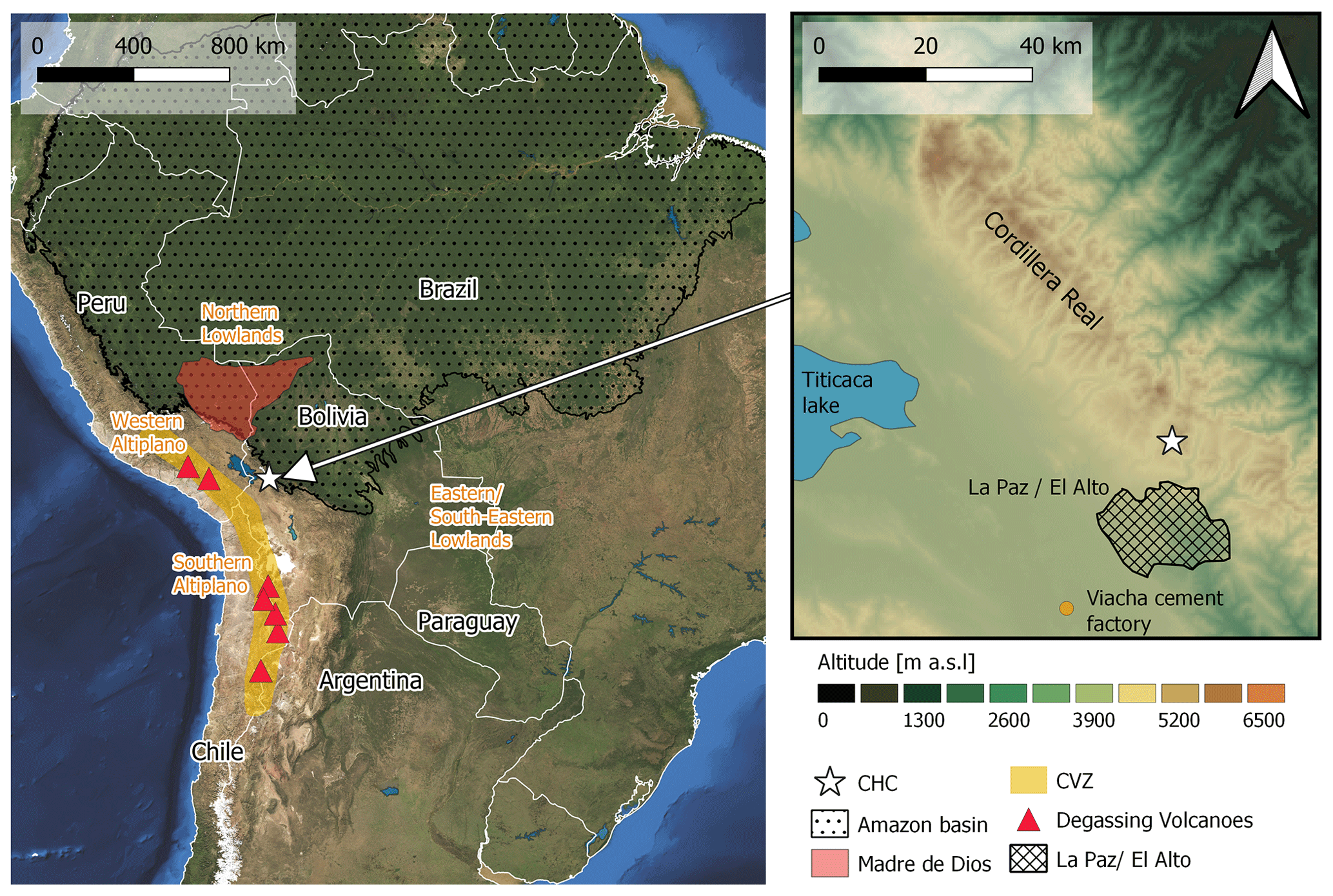
Figure 1 The left panel shows a true-color satellite image (from Esri) of the location of CHC station (star) on the South American continent, with the “Madre de Dios” watershed shaded in red, the Central Volcanic Zone (CVZ) shaded in yellow, and the extent of the Amazon Basin shown using a dotted surface (Amazon shapefile: http://worldmap.harvard.edu/data/geonode:amapoly_ivb, last access: 23 October 2020). Air mass origins, as used in this work, are shown in orange. Selected degassing volcanoes in the CVZ are shown as red triangles: Sabancaya, Ubinas, Ollagüe, San Pedro, Putana, Lascar, and Lastarria (from north to south). The right panel is a zoomed in map with color-coded elevation. The hatched area represents the La Paz–El Alto metropolitan area, and the orange dot shows the cement factory “Cemento Soboce” in the town of Viacha.

CHC is relatively close (∼ 300 km distance) to the “Madre de Dios” watershed, a known ASGM hot spot (Beal et al., 2013; Diringer et al., 2015, 2019). Apart from this prominent region, many other ASGM sites exist in the Bolivian, Peruvian, and Brazilian lowlands, but little exact information is available due to their intrinsically poorly documented and unregulated nature.

Finally, starting in northern Chile, extending all along the Bolivia–Chile border and reaching into Peru, we find the Central Volcanic Zone (CVZ), where several volcanoes have been reported to be actively degassing, both to the south (Tamburello et al., 2014; Tassi et al., 2011) and to the west of CHC (Moussallam et al., 2017). This entire volcanic arc showed SO₂ emissions that were above the long-term average in 2015 (Carn et al., 2017).

2.2 Data

2.2.1 TGM measurements

Atmospheric total gaseous mercury (TGM) was measured at CHC GAW station from July 2014 to February 2016, using a Tekran Model 2537A analyzer (Tekran Inc., Toronto, Canada). Concentrations are expressed in nanograms per cubic meter at standard temperature and pressure (STP; 273.15 K, 1013.25 hPa). The instrument is based on mercury enrichment on a gold cartridge, followed by thermal desorption and detection by cold vapor atomic fluorescence spectroscopy (CVAFS) at 253.7 nm (Fitzgerald and Gill, 1979; Bloom and Fitzgerald, 1988). Switching between two cartridges allows for alternating sampling and desorption and, thus, results in full temporal coverage of the atmospheric mercury measurement. During the 20-month measurement period, the instrument was automatically calibrated every 4 d on average, using an internal mercury permeation source. The latter was annually checked against manual injections of saturated mercury vapor taken from a temperature-controlled vessel, using a Tekran 2505 mercury vapor calibration unit and a Hamilton digital syringe, and following a strict procedure adapted from Dumarey et al. (1985). Atmospheric air, sampled through an unheated and UV-protected polytetrafluoroethylene (PTFE) sampling line and inlet installed outside at 6 m a.g.l. (above ground level), was previously filtered by two 4.5 and 0.5 µm 47 mm filters before entering the Tekran, in order to prevent any particulate matter from being introduced into the detection system. The instrument worked with a flow rate of 0.7 L min⁻¹ at STP, which was permanently checked by a Tylan calibrated and certified internal mass flow meter. In addition, the flow rate was controlled manually with an external volumetric flow meter every 3 months.

The range of TGM concentrations measured during the entire period (43 732 data points) was 0.42 to 4.55 ng m⁻³, with the detection limit of the instrument being below 0.1 ng m⁻³. Given a time resolution of 15 min and a sampling flow rate of 0.70 L (STP) min⁻¹, this corresponds to mercury mass loads on the gold cartridges of between ∼ 5 and ∼ 48 pg per cycle (average collection of 11.3 pg) with 54 % and 81 % of the mercury loading per cycle being above 10 and 8 pg, respectively.

As the instrument is limited by local low pressure (540 mbar) at the high-altitude CHC station and considering the range of detected concentrations, the default peak integration parameters were quickly optimized to avoid any low bias of measurements due to the internal Tekran integration procedure (Ambrose, 2017; Slemr et al., 2016; Swartzendruber et al., 2009). Non-linear integration responses for mercury mass loading below 10 pg per cycle have been observed with non-adjusted parameters that control the detection of the end of the peak (NBase and VBase). The latter were improved as stated by Swartzendruber et al. (2009), ensuring high-quality detection conditions at this very atypical atmospheric station, the highest in the world, where the Tekran analyzer, as well as all measurement systems, run under very stringent environmental conditions.

To ensure the comparability of the mercury measurements regardless of the study site, the Tekran instrument has been operated according to the GMOS (Global Mercury Observation System) standard operating procedures (SOP; Munthe et al., 2011), in accordance with best practices on measurements adopted in well-established regional mercury monitoring networks (CAMNet, AMNet). Raw dataset, routine, and exceptional maintenance and monitoring files were compiled and processed by software developed at the IGE (Institute of Environmental Geosciences) and specifically designed to quality assure and quality control atmospheric mercury datasets in order to produce clean TGM time series. In this automated process, the raw dataset is compared against potential flags corresponding to more than 40 criteria that specifically refer to all operation phases related to the calculation of mercury concentrations and calibration (D'Amore et al., 2015). Each raw observation is individually flagged depending on the result of each corresponding criterion and returns, as a temporary output, a flagged dataset (valid, warning, and invalid). Inclusion of all field notes, implying corrections and invalidations of data regrouped in the flagged dataset step, as well as a clarification step by the site manager according to their knowledge allows for the production of a complete quality-assured and quality-controlled dataset according to the initial temporal acquisition resolution.

2.2.2 CO measurements

The atmospheric CO mixing ratio was measured at CHC with a 1 min integration time using a non-dispersion cross-modulation infrared analyzer (model APMA-370, HORIBA Inc.). The sample air was pulled from the outside at about 0.8 L min⁻¹ through a 2 m Teflon line. The lower detectable limit is 50 [nmol mol⁻¹], and the instrument was set up to measure in the scale of 0–5 [µmol mol⁻¹].

2.2.3 eBC measurements

At CHC, the atmospheric black carbon mass concentration is continuously measured by a multi-angle absorption photometer (MAAP) (model 5012, Thermo Scientific). The MAAP is a filter-based instrument that utilizes a combination of light reflection and transmission measurements at 637 nm (Müller et al., 2011) together with a radiative transfer model to yield the black carbon concentration using a constant mass absorption cross section of 6.6 m² g⁻¹ (Petzold and Schönlinner, 2004). As black carbon by definition cannot be unambiguously measured with filter-based instruments, it is customary to call the measured light-absorbing constituent equivalent black carbon (eBC) (Bond and Bergstrom, 2006). The sample air is conducted to the instrument through a 1.5 m conductive tube from the main inlet that is equipped with an automatic heating system and a whole-air sampling head. Data based on 1 min were recorded, and their hourly averages were used for the analysis given a detection limit of 0.005 µg m⁻³.

2.2.4 CO₂ measurements

Atmospheric CO₂ concentrations have been measured with a cavity ring-down spectrometer (CRDS) from Picarro (model G2301). This analyzer measures the concentration of CO₂, CH₄, and H₂O every 2–3 s. The analyzer was calibrated upon a suite of four calibrated compressed air cylinders provided by LSCE (Laboratory for Sciences of Climate and Environment) central laboratory (calibrated against the WMO scale) every 2–4 weeks, and quality control of the data was ensured by regular analysis of two target gases (with known and calibrated concentrations); one short-term target gas analyzed for 30 min at least twice a day and one long-term target gas analyzed for 30 min during the calibration procedure. Those regular measurements indicate a repeatability of 0.04 ppm. Ambient air is pumped from the roof platform through Dekabon tubing. The Picarro analyzer enables the measurement of atmospheric moisture content, which is used to correct the measured greenhouse gas (GHG) concentrations.

2.2.5 Hourly data averaging

We generally worked with hourly averages to allow for easy synchronization of measurements from different instruments. Hourly averages were based on the arithmetic mean of all data taken within an hour (starting at 0 and ending at 59 min). In the case of TGM, if more than 50 % of the singular data points within an hour were invalid (missing data or flagged as bad data), a no-data value was assigned to the respective hourly average and it was excluded from further analysis. In the case of CO₂, where measurements were obtained every few seconds, the hourly averages were based on previously computed minute averages.

2.2.6 Uncertainties and confidence intervals

All uncertainties of mean concentrations are expressed as 2 times the standard error of the mean (SEM), giving approximately a 95 % confidence interval when comparing subsets of data measured at CHC, under the assumption of constant systematic uncertainty. When comparing CHC data to other stations, we suggest using this value only if it is higher than the average estimated systematic uncertainty for the respective instrument. In the case of the Tekran analyzer, this is about 10 % of the measured value (Slemr et al., 2015).

The approximately 95 % confidence interval for medians in box plots, shown as a notch, is based on the following equation: ${\mathrm{median}}_{\mathrm{upper}/\mathrm{lower}}=\mathrm{median}\pm \mathrm{1.58}\cdot \frac{\mathrm{IQR}}{\surd n}$ , where IQR is the interquartile range, and n is the number of data points (McGill et al., 1978). As in the case of the SEM, we advise using the systematic uncertainty of the respective instrument when carrying out comparisons to other measurement sites.

Robust linear models (iteratively reweighted least squares) and their confidence intervals at a level of 95 % were computed using the “MASS” package for R (Venables and Ripley, 2002). Confidence intervals are displayed in square brackets.

2.2.7 Solar-induced fluorescence (SIF) – SIFTER

As a remotely sensed proxy for vegetation activity, we examined satellite data on solar-induced fluorescence (SIF). More concretely, the SIFTER v2 product described in Koren et al. (2018), provided under the DOI https://doi.org/10.18160/ECK0-1Y4C, and based on the TEMIS SIFTER v2 product, which uses GOME-2A data (Kooreman et al., 2020). SIF has been previously shown to be a good proxy for photosynthetic activity and gross primary production (GPP) (Frankenberg et al., 2011; Koren et al., 2018; Qiu et al., 2020; Sanders et al., 2016; Zhang et al., 2014). Particularly, satellite-obtained SIF is thought to be a more direct measure of plant chemistry than retrieval products based on spectral reflectance, such as the normalized difference vegetation index (NDVI) and the enhanced vegetation index (EVI) (Luus et al., 2017; Zhang et al., 2014). Following the same procedure as described in Koren et al. (2018), we accounted for GOME-2A sensor degradation by linear detrending and obtained an identical time series for the average monthly SIFTER over the entire (legal) Amazon rainforest, which we later used as a proxy for Amazon GPP to establish a connection between the variation in mercury levels and vegetation activity. (The Amazon mask can be found at https://doi.org/10.18160/P1HW-0PJ6.)

2.2.8 The Oceanic Niño index (ONI)

To assess the possible influence of the El Niño–Southern Oscillation (ENSO), we deployed the ONI, which is based on the sea surface temperature (SST) anomaly in the Nino 3–4 region (5^∘ N–5^∘ S, 170–120^∘ W). It is the main index used by the National Oceanic and Atmospheric Administration (NOAA) to evaluate the strength of ENSO events and can be obtained at https://origin.cpc.ncep.noaa.gov/products/analysis_monitoring/ensostuff/ONI_v5.php, last access: 23 October 2020.

2.3 Definition of seasonal periods

Air masses arriving at CHC have been reported to show a strong seasonal dependency, both in their origin and the magnitude of biomass burning (BB) influence (Chauvigné et al., 2019; Rose et al., 2015). As in previous studies about CHC station, we grouped the year into three main seasonal periods (“seasons”), which we define as follows:

1. The part of the dry season from May to the end of July that is not strongly impacted by BB (hereafter shortened to “dry season”); this season is climatologically characterized by predominant highland (Altiplanic) influences and a low moisture content, and it is part of austral winter.

2. The BB season that takes place from August to the end of October. During this time of the year, forest fires tend to be most common in the region (Fig. A1; Ulke et al., 2011; Morgan et al., 2019), and important BB influences are registered at CHC. Initially, this season is climatologically comparable to the dry season, but it experiences quickly increasing lowland influences as time proceeds.

3. The wet season that takes place from December to the end of March. During this time of the year, lowland (Amazonian) influences and moisture content are highest, and BB is mostly insignificant. This season coincides with austral summer.

Furthermore, we considered the remaining months of the year, April and November, to be “transition months” between the mentioned seasons and did not include them in the seasonal analysis.

2.4 Air mass origin at the regional scale

To identify common pathways of air mass origin and transport, we used the same set of HYSPLIT back trajectories as already described in Chauvigné et al. (2019). Briefly, for every hour of the day, a 96 h runtime HYSPLIT back trajectory (Stein et al., 2015) was computed for each of nine arrival points located at 500 m above ground and within a 2 km × 2 km square grid around the station. The input meteorological fields for the HYSPLIT simulations were obtained from ERA-Interim and dynamically downscaled using the Weather Research and Forecasting (WRF) model to increasing nested spatial resolutions of 27, 9.5, 3.17, and, finally, 1.06 km to account for the complex topography of the site.

Additionally, we worked with the air mass classification results introduced in the same work, obtained by applying k-means clustering to the temporal signatures (number of back-trajectory piercings per month of the year) of geographical cells on a log-polar grid (Chauvigné et al., 2019). Their method, applied to HYSPLIT back trajectories between January 2011 and September 2016, yielded six prevalent clusters of air mass origin. They are shown in Fig. 2 and can be briefly described as follows:

• Cluster C1 – northern lowlands; air masses of Amazonian origin, which take a southward turn after hitting the Andes (Ulke et al., 2011). This cluster includes the very ASGM-active Madre de Dios watershed.

• Cluster C2 – eastern and southeastern lowlands. This cluster includes scrubland like the Dry Chaco region between Bolivia and Paraguay as well as the Pantanal wetland at the eastern frontier to Brazil.

• Cluster C3 – northern Chile and southern Altiplano. This cluster includes actively degassing volcanoes of the CVZ (Tamburello et al., 2014; Tassi et al., 2011) and the La Paz valley.

• Cluster C4 – eastern edge of the Altiplano. This cluster includes air masses passing to the east of Lake Titicaca.

• Cluster C5 – western Altiplano. This cluster includes Lake Titicaca, the Peruvian highland, and the Pacific Ocean as well as passing over parts of the CVZ (Moussallam et al., 2017).

• Cluster C6 – this cluster includes cloud forest at the northeastern edge of the Cordillera Real.

By following Eq. (1), Chauvigné et al. (2019) computed the relative influence of the six clusters, expressed as a percentage, for each hour of the day.

$$\begin{array}{}\text{(1)}& P_i\left(t\right)={\displaystyle \frac{{\sum }_{k\in C_i}{n}_k\left(t\right)w_k}{{\sum }_{k\in C_n}{n}_k\left(t\right)w_k}}\cdot \mathrm{100}\mathit{\%},\end{array}$$

where P_i(t) is the relative influence of cluster i for the hour of trajectory arrival t, C_i is the set of all cells assigned to cluster i, C_n is the set of all cells in the grid (C_i⊆C_n), n_k(t) is the total number of pixel piercings for cell k by any of the nine trajectories arriving simultaneously at CHC at hour t, and w_k is the relative weight of cell k as a function of mean residence time and distance to CHC.

Air masses arriving at CHC are usually composed of a mix of the six clusters, and in only very few cases, the relative influence of one single cluster reaches 100 %. Thus, we applied a selection threshold to assign hourly measurements at CHC to one single cluster: if the percentage of relative cluster influence as calculated by Eq. (1) exceeded the selection threshold for any of the six clusters, we considered the latter to be the “dominant cluster” and assigned it to all measurements taken at CHC during the hour of back-trajectory arrival. All data obtained at arrival times for which none of the clusters were dominant were excluded from this analysis. Unless stated otherwise, we chose a threshold of 70 % to find a compromise between unambiguity with respect to air mass origin and the data availability, as the latter decreases rapidly with higher selection thresholds, especially for the weaker clusters C2, C3, C4, and C6. In a nutshell, if the set of nine back trajectories arriving simultaneously at the station spent over 70 % of its time within cells assigned to one single cluster, we considered the latter to be the dominant cluster (at a selection threshold of 70 %).

2.5 Pollution maps

To further visualize the link between air mass origin and TGM concentrations, we produced what we call “pollution maps”. These are based on the same set of HYSPLIT back trajectories introduced previously and were computed with the following procedure: first, for each single back trajectory, we assigned the TGM concentration at back-trajectory arrival to each of its endpoints (each back trajectory consists of 96 trajectory endpoints, one for every hour of its runtime). We then defined a geographical grid and grouped together all endpoints (defined in space by latitude, longitude, and elevation over ground level) falling into the same grid cell. Finally, for each grid cell, we calculated the arithmetic mean of all TGM concentrations assigned to the corresponding grouped endpoints.

It has to be highlighted that this procedure permits the multiple counting of the same measured TGM concentration in the calculation of one single grid cell mean. This happens if more than one endpoint of the same trajectory or endpoints of different trajectories with the same arrival time fall into the same geographical grid cell. We considered this sort of inherent weighting to be desirable, as it gives greater weight to TGM concentrations assigned to air masses passing an extended period of time over the grid cell in question. However, to assure a certain degree of statistical significance, we excluded those grid cell means based on less than 10 independent data points on TGM concentration (n<10).

To account for growing trajectory uncertainty with increasing distance to the receptor site (CHC), to avoid the misinterpretation of a pollution map as a satellite image, and to allow for easy visual comparison between pollution maps and air mass clusters, we used the exact same CHC-centered log-polar grid as deployed in Chauvigné et al. (2019).

Figure 2 Air mass cluster definition as obtained by Chauvigné et al. (2019). The log-polar coordinate system is centered on CHC (white dot). The cells are shaded according to the square root of weight, which is a function of residence time and distance to CHC. Dashed range circles show the distance to CHC in degrees, which can be converted to kilometers using the conversion factor 1^∘ = 108.6 km, with an error below 3 % in the whole domain. Black lines show the borders between countries.

With the goal of focusing on potential sources and sinks acting close to the surface, we excluded all trajectory endpoints with an elevation greater than 1000 m a.g.l. from this analysis (assuming an average boundary layer height of 1000 m a.g.l.). This essentially means that only trajectories passing at low altitudes over a grid cell have an influence on the TGM average calculated for the cell.

3 Results

3.1 TGM concentrations under normal and ENSO conditions – seasonality

A summary of the monthly averaged TGM concentrations is presented in Fig. 3a. The data show an overall rising trend during the measurement period. As this trend exhibits a striking similarity to the evolution of the ONI (Fig. 3c), we suggest an important ENSO influence on TGM measured at CHC. This will be discussed in detail in an upcoming publication. In the present paper, we labeled the last 9 months of our measurement period (June 2015–February 2016) with ONI >1 as ENSO conditions (ECs) and excluded them from most of our analysis as not representative of normal conditions (NCs).

We obtained a mean TGM concentration of 0.89±0.01 ng m⁻³ for NCs and a significantly higher mean of 1.34±0.01 ng m⁻³ for ECs ($p<\mathrm{2.2}\times {\mathrm{10}}^{-\mathrm{16}}$, Mann–Whitney test). For both NCs and ECs, we can observe a similar seasonal pattern, with low TGM concentrations during the dry season, rising TGM concentrations during BB season, and the highest TGM concentrations at the beginning of the wet season (Fig. 3a, b). Under NCs, TGM concentrations started declining again in January, whereas this was not observable for ECs.

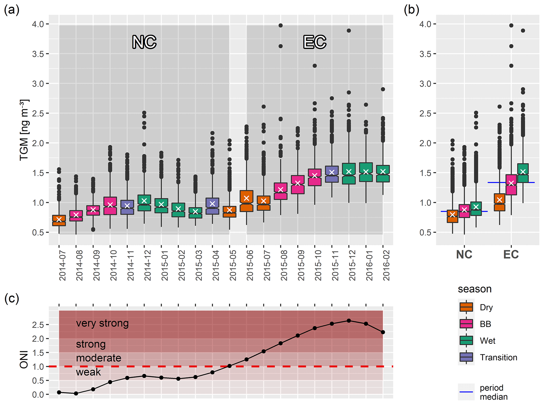
Figure 3 (a) Time evolution of TGM at CHC during the entire measurement period. Notches display 95 % confidence intervals for the median, means are shown as white crosses, and normal condition (NC), and ENSO condition (EC) time intervals are shown using shaded boxes. Whiskers extend to the highest and lowest data points within the interval [1st quartile – 1.5 IQR, 3rd quartile + 1.5 IQR], and values outside of this range are shown as black dots. (c) Evolution of the ONI during the same period alongside NOAA definitions of the strength of ENSO phases. The dashed red line shows the boundary value that we used here to separate NCs from ECs (ONI = 1). (b) Seasonality of TGM in CHC during NCs and ECs, where transition months are excluded. Horizontal blue lines show the total median of the respective period.

3.2 Diel cycle, urban influence, and nearby contamination

Given that the metropolitan area of La Paz–El Alto is located less than 20 km downhill of the measurement site, we investigated the possibility of a statistically important urban influence on TGM measurements. Previous studies (Andrade et al., 2015; Wiedensohler et al., 2018) have shown a significant influence of regional sources and the nearby metropolitan area on CO and eBC concentrations measured at the station. A marked increase in average CO and eBC diel patterns (Fig. 4b, c), starting at around 09:00 LT, has been linked to the arrival of the Altiplanic planetary boundary layer, vehicle traffic, and urban contamination in general. In contrast, the diel cycle of TGM (Fig. 4a) is qualitatively different, with no marked increase associated with the arrival of the boundary layer but, instead, slightly lower TGM values between about 07:00 and 19:00 LT, which coincides well with the typical hours of sunlight and general boundary layer influence. The absence of a diel pattern driven by traffic and urban pollution is not very surprising, as there are no major sources of mercury in the poorly industrialized cities of La Paz and El Alto, and domestic heating is nearly absent. The only potential local sources we suggest could be the occasional waste burning by individuals and a cement factory located about 40 km southwest of the station (Cemento Soboce; 16.647^∘ S, 68.317^∘ W; Fig. 1). Either way, the magnitude of urban- or traffic-related TGM contamination at CHC appears to be negligible.

Figure 4 The left column shows the median diel cycles of (a) TGM, (b) CO, and (c) eBC for NCs. The limits of the gray shaded area correspond to the 25th and 75th percentiles. Vertical lines represent sunrise and sunset hours for the summer solstice in the wet season (solid line) and the winter solstice in the dry season (dashed line). The typical arrival time of the urban-influenced Altiplanic planetary boundary layer (PBL) is highlighted in orange. The right column shows the daily averaged (25th percentile, median, 75th percentile) (d) TGM, (e) CO, and (f) eBC during June 2015.

One event where TGM concentrations were clearly driven by nearby anthropogenic pollution was Saint John's Eve, the night between the 23 and 24 June 2015, where TGM concentrations peaked alongside CO and eBC concentrations (Fig. 4d, e, f). During nights around this traditional festivity, numerous bonfires are lit and fireworks are launched in the region. In these bonfires, in addition to untreated wood, garbage, old furniture, and other objects are also burned. The relatively high mean TGM concentrations during June 2015, compared with May and July 2015 (Fig. 3a), could be explained by the Saint John event alone, especially if we consider the relatively poor data coverage during that month (only 21 out of 30 daily averages available) and the resulting greater weight given to a few days (∼ 6 d) of elevated concentrations.

3.3 Spatial differences in TGM concentrations – air mass origins

The evident seasonal pattern in transportation pathways towards CHC is visualized in Fig. 5. The most important air mass clusters under NCs, measured by mean relative influence and appearance as the dominant cluster, were the Amazonian C1 and Altiplanic C5 clusters (Fig. 5c, d).

Figure 5 (a) Total number of back-trajectory piercings per pixel for the NC period and its seasons, normalized through division by the maximum, so that “1” corresponds to the most frequently pierced pixel. Note the logarithmic color scale. The polar grid has constant angular but variable radial resolution and is centered on CHC (white dot). Dashed range circles show the distance to CHC in degrees, which can be converted to kilometers using the conversion factor 1^∘ = 108.6 km, with an error below 3 % in the whole domain. (b) Reminder of the cluster definition as obtained by Chauvigné et al. (2019), using the same polar grid. (c) Weighted mean relative influence (%) for the six clusters during the entire NC period and its seasons. (d) Number of cluster appearances as “dominant cluster” at a threshold of 70 %. Note the logarithmic y axis.

In the dry season, most of the air masses arriving at the station were western Altiplanic (C5), passing over the Peruvian highlands and Lake Titicaca. This changed in the wet season with a clear shift towards predominantly Amazonian and lowland air masses (northerly C1 and easterly C2). The Altiplanic (C5) cluster was weak during that time of the year (mean relative influence <10 %).

With much less seasonal variation, southerly Altiplanic air (Cluster C3) arrived occasionally from the border between Bolivia and Chile after passing through parts of the CVZ and – frequently – the urban area of La Paz–El Alto. Altiplano–lowland interface clusters C4 and C6 were relatively weak throughout the year and appeared very infrequently as dominant clusters at a threshold of 70 % (Fig. 5d).

As shown in Fig. 6, we tried to infer potential source and sink regions of TGM through clustering results and a pollution map (based on an endpoint cutoff altitude of 1000 m a.g.l., as described in Sect. 2; pollution map results at different cutoff altitudes are given in Appendix B). Based on all NC data, northern Amazonian and southern Altiplanic air masses, especially those passing over or close to reportedly degassing volcanoes south of CHC (Ollagüe, San Pedro, Putana, Lascar, and Lastarria; Tamburello et al., 2014; Tassi et al., 2011), carried the highest mean TGM concentrations (around 0.94±0.02 and 1.08±0.08 ng m⁻³, respectively), whereas western Altiplanic and southeastern lowland air masses showed the lowest mean TGM concentrations (around 0.80±0.02 and 0.85±0.02 ng m⁻³, respectively; Fig. 6a). By grouping data by season (i.e., wet, dry, and BB), more detailed information could be extracted (Fig. 6b). Only the northern Amazonian cluster (C1) showed both the highest CO and TGM concentrations during the BB season (arithmetic means of 150±5 ppbv and 0.99±0.04 ng m⁻³, respectively). Western Altiplanic cluster C5 exhibited the lowest mean TGM concentrations in the dry season (0.77±0.01 ng m⁻³) and the highest TGM concentrations in the wet season (0.93±0.07 ng m⁻³). The mean concentration in the southern Altiplanic cluster (C3) was 0.92±0.05 ng m⁻³ with no significant differences between the wet and BB season (p=0.76, Mann–Whitney test). Eastern lowland cluster C2 only contributed as a dominant cluster during the wet season, but it showed the lowest mean TGM concentrations by far during that time of the year (0.82±0.02 ng m⁻³). The seasonal change in transport pathways becomes evident if we consider that only Altiplanic cluster C5 contributed significantly as a dominant cluster (at a selection threshold of 70 %) in the dry season. No useful information could be extracted about Altiplano–lowland interface clusters C4 and C6, as their relative influence throughout the year was low (Fig. 5c, d).

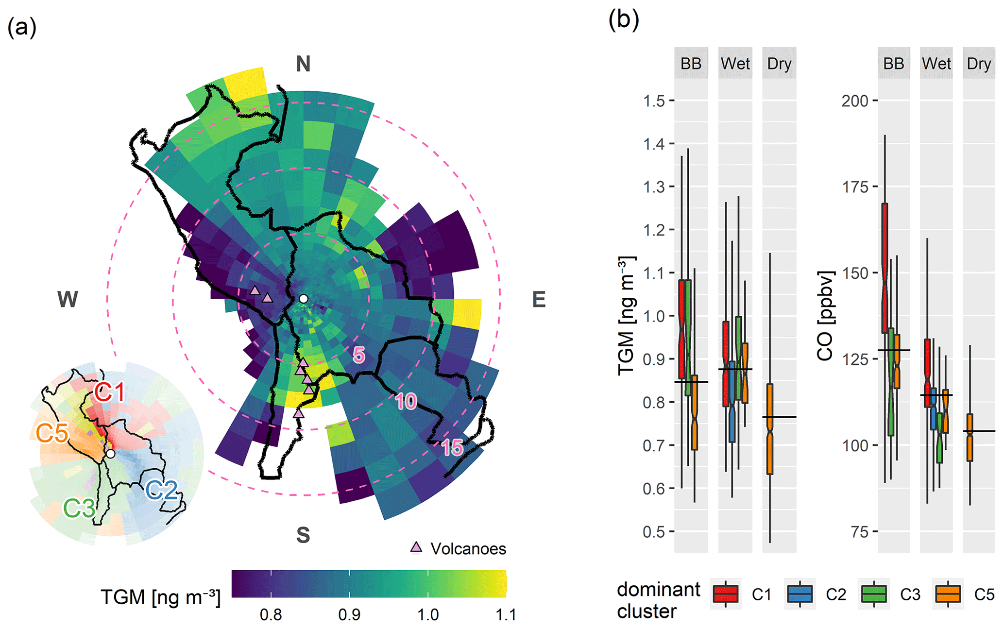
Figure 6 (a) Pollution map based on TGM data taken during the entire NC period. The polar grid is centered on CHC (white dot). Dashed range circles show the distance to CHC in degrees, which can be converted to kilometers using the conversion factor 1^∘ = 108.6 km, with an error below 3 % in the whole domain. Trajectory endpoints with an elevation >1000 m a.g.l. and cells with less than 10 data points (n<10) were excluded. The color scale was capped at the limits. Pink triangles show selected degassing volcanoes in the CVZ: Sabancaya, Ubinas, Ollagüe, San Pedro, Putana, Lascar, and Lastarria (from north to south). The small map shows the air mass cluster definition. (b) TGM and CO concentrations for different seasons and clusters during the NC period, based on a cluster selection threshold of 70 %. Groups with n<10 are excluded from the plot. Horizontal lines show seasonal medians based on all NC data. Whiskers extend to the highest and lowest data point within the interval [1st quartile – 1.5 IQR, 3rd quartile + 1.5 IQR], and values outside of this range are not shown.

4 Discussion

4.1 TGM means and seasonality

TGM concentrations under NCs (11-month mean from July 2014 to May 2015: 0.89±0.01 ng m⁻³) were about 10 % to 15 % lower, compared with subtropical sites of the Southern Hemisphere such as Amsterdam Island in the remote southern Indian Ocean (37.7983^∘ S, 77.5378^∘ E; 55 m a.s.l.) with a GEM annual mean of 1.034±0.087 ng m⁻³ (from 2012 to 2017; Angot et al., 2014; Slemr et al., 2020) and the Cape Point GAW station in South Africa (34.3523^∘ S, 18.4891^∘ E; 230 m a.s.l.) with a GEM annual mean around 1 ng m⁻³ (from 2007 to 2017; Martin et al., 2017; Slemr et al., 2020). No GEM annual mean below 1 ng m⁻³ was observed at these two atmospheric mercury monitoring stations in 2014 and 2015, corresponding to the CHC NC period. Mean annual GEM concentrations of 0.95±0.12 ng m⁻³, i.e., close to but still higher than the NC TGM concentrations, were observed from 2014 to 2016 (Howard et al., 2017) at the Australian Tropical Atmospheric Research Station (ATARS) in northern Australia (12.2491^∘ S, 131.0447^∘ E; near sea level), whereas the midlatitude Southern Hemisphere site of global GAW Cape Grim (40.683^∘ S, 144.689^∘ E; 94 m a.s.l.) exhibited annual mean concentrations of around 0.86 ng m⁻³ (from 2012 to 2013; Slemr et al., 2015). TGM concentrations at CHC are well in line with measurements on the continent performed at Lake Titicaca, at around 3800 m a.s.l. and about 60 km west from our site (not continuously measured between 2013 and 2016: TGM mean of 0.82±0.20 ng m⁻³ in the dry and 1.11±0.23 ng m⁻³ in the wet season; Guédron et al., 2017), and in Patagonia (from 2012 to 2017, GEM mean of 0.86±0.16 ng m⁻³; Diéguez et al., 2019).

CHC TGM under NCs showed a marked seasonality, with the lowest TGM during the dry season (0.79±0.01 ng m⁻³), increasing values during BB season (0.88±0.01 ng m⁻³), and the highest TGM during the wet season (0.92±0.01 ng m⁻³). This behavior is congruent with the results from Guedrón et al. (2017), even though the seasonal difference did not appear statistically significant for the latter. The marked seasonality at the CHC site is in contrast to what has been observed at some subtropical and midlatitude sites in the Southern Hemisphere, both in terms of the amplitude and the seasonal average level (Howard et al., 2017; Slemr et al., 2015, 2020).

This seasonality is likely a product of the superposition of several important drivers, coupled with seasonal changes in transportation pathways (Fig. 5). In the next sections, we further explore the potential role of BB-related Hg emissions, the Amazon rainforest, and the Pacific Ocean. We also explore volcanoes in the CVZ and ASGM as atmospheric Hg sources without specific seasonality but with possible influence on CHC TGM levels.

4.2 Biomass burning and the TGM $/$ CO emission ratio

4.2.1 Biomass burning influence

BB is an important source of atmospheric mercury (Obrist et al., 2018; Shi et al., 2019). Friedli et al. (2009) estimated global mercury emissions from BB and found a high contribution from South America (13±10 Mg_Hg yr⁻¹ for its Northern hemispheric and 95±39 Mg_Hg yr⁻¹ for its Southern hemispheric regions). Michelazzo et al. (2010) measured Hg stored in Amazonian vegetation before and after fires, finding that mercury emissions originated mostly from the volatilization of aboveground vegetation and the plant litter layer (O-horizon). Very recently, Shi et al. (2019) showed, among others, high Hg emissions in northern Bolivia, a region overlapping very well with the source region of Amazonian cluster C1. Indeed, for this cluster, whose BB influence had already been confirmed by Chauvigné et al. (2019), we found both the highest CO and TGM concentrations during the BB season (see Figs. 6b and A1); these concentrations were significantly higher than during the rest of the NC period in both cases ($p<\mathrm{2.2}\times {\mathrm{10}}^{-\mathrm{16}}$ and p<0.0008, respectively, Mann–Whitney test).

In order to further explore the link between BB and TGM in our data, independently of computed HYSPLIT back trajectories, we used the combination of CO and eBC data measured in situ as tracers for distinct combustion sources and transport times (Choi et al., 2020; Subramanian et al., 2010; Zhu et al., 2019). We grouped CO and eBC data into eight percentile groups each, ranging from the 0th to 100th in steps of 12.5 % (CO range: 37– 336 ppbv; eBC range: 0–5.09 µg m⁻³). Based on these groups we produced an 8×8 grid, where each cell (“pollution signature”) corresponds to a combination of CO and eBC concentration intervals. We then calculated the median TGM concentration for each pollution signature in the grid (Fig. 7a).

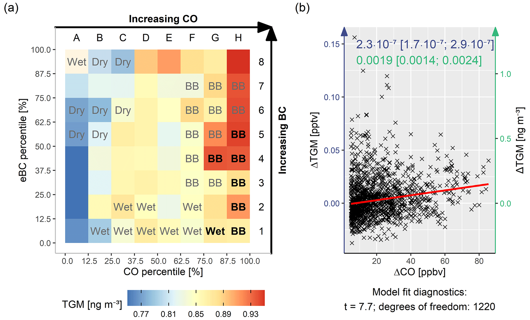
Figure 7 (a) TGM medians for different combinations (“pollution signatures”) of eBC and CO concentrations, each split into eight percentile groups ranging from 0 % to 100 %, so that the first group contains data below the 12.5th and the last group contains data above the 87.5th percentile. All data were taken during NCs at CHC. Gray (black) letters mark signatures whose data falls into the respective season more than 51 % (85 %) of the time. Cells with n<30 are shaded out proportionally. The color scale is centered on the NC median and capped at the limits. (b) The red line shows the robust linear model (iteratively reweighted least squares) between Δ TGM and ΔCO, defined as the difference between actual measurement and assumed background concentrations, for all data in pollution signatures with a >51 % occurrence during the NC BB season (all cells with gray or black “BB” letters in panel a). The resulting slope, which can be interpreted as the TGM $/$ CO emission ratio, is given in units of ppbv_TGM ppbv${}_{\mathrm{CO}}^{-\mathrm{1}}$ (blue) and (ng m⁻³)_TGM ppbv${}_{\mathrm{CO}}^{-\mathrm{1}}$ (green) with its 95 % confidence interval.

Pollution signatures showed a clear seasonal trend. During the dry season, eBC tended to be high and CO was low. TGM concentrations tended to increase with rising CO concentrations, whereas even highly eBC enriched air masses had very low TGM concentrations in the absence of CO (for example, cells B-8 and C-8). The latter suggests that urban pollution originating from traffic does not act as an important driver of atmospheric Hg measured at CHC, in agreement with the TGM diel pattern (Fig. 4a), which shows no TGM increase upon arrival of the frequently traffic-influenced planetary boundary layer and a simultaneous increase in eBC. During the wet season, eBC at CHC station tended to be very low, which is likely linked to the increased wet deposition of particulate matter during that season, whereas CO concentrations were very variable. The absence of a visible pattern concerning TGM in those pollution signatures suggests that TGM concentrations during the wet season are either not importantly affected by combustion of any kind or that different combustion sources are indistinguishable through their eBC and CO signatures around this time.

Finally, BB season pollution signatures generally showed very high CO and highly variable eBC concentrations. Within those signatures, TGM concentrations clearly increased with rising CO concentrations but did not depend strongly on eBC loadings, even though they tended to be lower in the case of very low eBC (e.g., H1, H3, G3, F3, with the exception of H2).

Considering that atmospheric lifetime is much shorter for BC (days to weeks; Cape et al., 2012; Park et al., 2005) than for CO (months; Khalil et al., 1990), especially under conditions of high wet deposition, we can expect that even if both eBC and CO are strongly co-emitted during BB events, air masses arriving at CHC should be significantly enriched in CO alone after a few days of transport. Thus, we can interpret the steadily high CO but comparatively low eBC loading of air masses with these pollution signatures as the result of an important BC deposition (wet and dry) during the transport between pollutant source and receptor site regions, either due to precipitation favoring wet deposition or a transport time of at least a few days. As the La Paz–El Alto metropolitan area, a hot spot for BC (Wiedensohler et al., 2018), is quite close to the station (<20 km) and transport time is, therefore, usually less than a few hours (see Fig. C1 in Appendix C), we can exclude urban influences as contributors to these pollution signatures and assign them to BB.

As median TGM concentrations were significantly higher in those pollution signatures occurring almost exclusively in the BB season (over 85 % of the time; Fig. 7a), compared with median NC concentrations (0.93 ng m⁻³ vs. 0.85 ng m⁻³, $p=\mathrm{1.7}\times {\mathrm{10}}^{-\mathrm{11}}$, Mann–Whitney test), we can conclude that there is an important influence of regional and continental BB on atmospheric mercury concentrations in the Bolivian Andes. This occurs only during a few months of the year (August–October), and it is mostly constrained to northern Amazonian air masses (cluster C1, remotely obtained CO concentrations in the cluster C1 source region are shown in Appendix A).

4.2.2 The TGM $/$ CO emission ratio

Having established a clear link between TGM and long-range-transported BB in our data, we aimed to estimate an average biomass burning TGM $/$ CO emission ratio on the continent. A first obstacle arises from the fact that BB is not the only source of TGM and CO measured at Chacaltaya. CO in particular is also readily emitted by anthropogenic activities (e.g., urban and traffic sources) in the surrounding Altiplano, as can be inferred from CO diel patterns (Fig. 4b) and previous work (Wiedensohler et al., 2018). As a consequence, simply computing TGM vs. CO in the entire unfiltered CHC dataset would not provide the BB-related TGM $/$ CO emission ratio, but a sort of “net emission ratio” over different sources of pollution with distinct emission ratios. To remove this distorting factor as much as possible and obtain a best guess biomass burning TGM $/$ CO emission ratio, we used the results from the previous section (pollution signatures): we attempted to isolate highly BB-influenced air masses by selecting only data with pollution signatures occurring preferentially during the BB season (>51 % of signature data taken in BB season; Fig. 7a) as BB representatives.

With this data selection performed, a linear model between TGM and CO could not yet be computed directly to obtain the emission ratio, as this would assume constant TGM and CO background conditions for the whole data selection. This is not a valid assumption, considering that the selection contains TGM data from different months and that a strong seasonal pattern was observed (Fig. 3a, b). To account for the changing background conditions, we first computed ΔTGM and ΔCO, which we defined as their measured concentration minus their assumed background concentration at the time of measurement. We expressed the TGM background through a 30 d running median, as it is clearly not constant during the year and seasonally shifting concentrations cannot be attributed to BB alone. This is different for CO, where we can assume that BB is the main driver of the seasonal signal in South America (Fig. A1a) and that the fluctuations in the background concentrations unrelated to BB are small in comparison to the BB-induced variations in measured concentrations at CHC (Fig. A1b). Thus, we used a simple median using all NC data to express the CO background (illustrated in Fig. A1b).

Finally, we determined the TGM $/$ CO emission ratio through the use of a robust linear regression (linear regression with iterative reweighting of points) between ΔTGM and ΔCO $(\mathrm{\Delta }\mathrm{TGM}=a+b\cdot \mathrm{\Delta }\mathrm{CO})$, obtaining a slope of $(\mathrm{2.3}\pm \mathrm{0.6})\times {\mathrm{10}}^{-\mathrm{7}}$ ppbv_TGM ppbv${}_{\mathrm{CO}}^{-\mathrm{1}}$ (Fig. 7b). This obtained emission ratio is robust towards changes in the parameters chosen for its calculation (sensitivity analysis presented in Appendix D) and is also in good agreement with previous results. Ebinghaus et al. (2007) deduced TGM $/$ CO emission ratios of $(\mathrm{1.2}\pm \mathrm{0.2})\times {\mathrm{10}}^{-\mathrm{7}}$ ppbv_TGM ppbv${}_{\mathrm{CO}}^{-\mathrm{1}}$ and $(\mathrm{2.4}\pm \mathrm{1})\times {\mathrm{10}}^{-\mathrm{7}}$ ppbv_TGM ppbv${}_{\mathrm{CO}}^{-\mathrm{1}}$ during CARIBIC flights over Brazil through measurements performed directly within fire plumes. Weisspenzias et al. (2007), using a more similar approach to ours, obtained results ranging from $(\mathrm{1.6}\pm \mathrm{1})\times {\mathrm{10}}^{-\mathrm{7}}$ ppbv_TGM ppbv${}_{\mathrm{CO}}^{-\mathrm{1}}$ for air masses originating in the Pacific Northwest, USA, up to $(\mathrm{5.6}\pm \mathrm{1.6})\times {\mathrm{10}}^{-\mathrm{7}}$ ppbv_TGM ppbv${}_{\mathrm{CO}}^{-\mathrm{1}}$ for those originating in industrial East Asia (numbers converted from (ng m⁻³)_TGM ppbv${}_{\mathrm{CO}}^{-\mathrm{1}}$ to ppbv_TGM ppbv${}_{\mathrm{CO}}^{-\mathrm{1}}$).

We observe a high scatter around our regression line of best fit, which is not surprising considering the distance from the receptor site to the source region and the resulting dilution and mixing. Thus, our TGM and CO data pairs do not correspond to the emissions of one single fire event, but many different fires and plumes as well as distinct times and conditions of aging. Thus, the obtained emission ratio should be interpreted as an average emission ratio of all fires in the northern Bolivian lowlands and the Amazon, after some aging has occurred.

4.3 The potential role of the vegetation in the TGM cycle

Globally, the role of vegetation in the mercury cycle is not yet completely understood, but there is much evidence pointing towards both reactive mercury (RM) deposition on leaf surfaces and a direct vegetation uptake of GEM. However, as highlighted in the literature review by Obrist et al. (2018), these pathways, especially the latter, are still not well constrained. Recently, Jiskra et al. (2018) reported a significant correlation between the remotely sensed NDVI vegetation tracer and GEM levels for individual sites in the Northern Hemisphere and argued that the absence or weakness of Hg seasonality in many sites in the Southern Hemisphere might be linked to its comparatively lower landmass and lower vegetation uptake. A similar point was made earlier by Obrist (2007), who proposed that vegetation uptake in the Northern Hemisphere might be partly responsible for the observed TGM seasonality in Mace Head, Ireland, which was a hypothesis based on the correlating seasonal patterns of atmospheric TGM and CO₂. Indeed, Ericksen et al. (2003) showed in mesocosm experiments that foliar Hg concentrations in gas chambers increase over time, leveling off after 2–3 months. Furthermore, they reported that roughly 80 % of the total accumulated Hg was stored in leaf matter and that soil Hg levels in the mesocosms had no significant effect on foliar Hg concentration – a piece of strong evidence that Hg is taken up directly from the atmosphere and not from the soil. Some very similar points were made by Grigal (2003), based on a review of Hg concentrations in forest floors and forest vegetation. Although it is assumed that vegetation acts as a net sink for atmospheric mercury (Obrist et al., 2018), Yuan et al. (2019) studied mercury fluxes in a subtropical evergreen forest and found isotopic evidence for a GEM re-emission process within leaves, partly counteracting the GEM uptake. They also reported a strong seasonality in mercury fluxes, with the highest GEM uptake in the growing/wet season. Considering these previous results, a modulation of continent-wide Hg levels through the Amazon rainforest is likely. Indeed, Figueiredo et al. (2018) already suggested that the Amazon rainforest acts as a net sink for atmospheric mercury, based on forest soil profiles.

To address such a possible link between TGM and vegetation in our data, we focused on lowland air masses only, as vegetation coverage in the Altiplano is sparse, GPP is low, and, consequently, no important vegetation sink effect is to be expected in Altiplanic air masses. Although both clusters C1 and C2 would qualify as lowland clusters passing over evergreen forests, C2 did not provide enough data to compute a useful series of monthly averages. Therefore, we selected Amazonian cluster C1 as the sole representative of Amazonian air masses. We explored two different proxies for a possible vegetation sink effect: CO₂ concentrations measured at CHC (detrended, assuming a Southern Hemisphere linear trend of 2 ppm yr⁻¹; trend based on AIRS (Atmospheric Infrared Sounder) CO₂ data between January 2010 and January 2015, averaged over whole South America) and satellite-obtained solar-induced fluorescence (SIFTER) averaged over the (legal) Amazon rainforest as a proxy for Amazon GPP. We then computed the slope of robust linear models for the combinations of TGM vs. CO₂ ($\mathrm{TGM}=a+b\cdot {\mathrm{CO}}_{\mathrm{2}}$) and TGM vs. SIFTER ($\mathrm{TGM}=a+b\cdot \mathrm{SIFTER}$) for C1 dominant air masses at increasing selection thresholds.

We observe an interesting trend, where the magnitude of the slopes becomes more important and slope uncertainty (compare to Sect. 2.2.6) decreases with an increasing Amazonian cluster C1 selection threshold (Fig. 8a, b). For thresholds of 70 % and 80 %, the resulting TGM vs. CO₂ slopes are 0.047 [0.035; 0.060] and 0.058 [0.041; 0.075] (ng m⁻³)_TGM ppm${}_{{\mathrm{CO}}_{\mathrm{2}}}^{-\mathrm{1}}$, respectively, whereas the resulting TGM vs. SIFTER slopes are −0.82 [−1, 11; −0.53] and −1.51 [−2.05; −0.97] (ng m⁻³)_TGM (mW sr⁻¹ m⁻² nm⁻¹)${}_{\mathrm{SIF}}^{-\mathrm{1}}$, respectively. Closer inspection of the corresponding TGM, CO₂, and SIFTER monthly averages at a C1 threshold of 70 % visualizes how both TGM and CO₂ reached their minimum in March 2015, coinciding with a peak in Amazon SIFTER as a proxy for Amazon GPP (Fig. 8d, e, f).

Figure 8 Slopes for (a) TGM vs. CO₂ ($\mathrm{TGM}=a+b\cdot {\mathrm{CO}}_{\mathrm{2}}$) and (b) TGM vs. SIFTER ($\mathrm{TGM}=a+b\cdot \mathrm{SIFTER}$) for robust linear models based on monthly averages, as a function of the chosen Amazonian cluster C1 threshold and the resulting selection of data. TGM and CO₂ monthly averages based on less than 30 data points (n<30) were excluded. Error bars show the 95 % confidence interval. The threshold used for the right-hand side of the plot (C1 mean influence >70 %) is shaded in blue. (c) The number of monthly averages available for the linear models at the respective threshold, excluding all monthly averages with n<30. The colors represent partitioning over the seasons. Examples of the time series of monthly averages are given for (d) TGM, (e) CO₂, and (f) SIFTER at a C1 selection threshold of 70 %. TGM and CO₂ reach their minimum when Amazon SIFTER peaks.

These results provide arguments for the presence of a vegetation-related Hg sink in Amazonian air masses, mainly during the wet season. As is to be expected from the comparatively low vegetation coverage in the Altiplano, no such correlation with CO₂ or SIFTER was found for air masses of Altiplanic origin. A clear downside to our approach here is that higher selection thresholds for C1 and, thus a cleaner selection of northern Amazonian air masses, provide a smaller number of monthly averages available for the linear models (Fig. 8c). Due to the seasonality of transport pathways towards the station (Fig. 5), the available monthly averages of C1-dominated air masses are not equally distributed over the year and mainly fall into the wet season. As these C1-dominated air masses very rarely fall into the dry season, we cannot make any assumptions about the relationship between TGM and vegetation tracers in lowland air masses during that time of the year.

Concerning our second vegetation proxy, remotely sensed SIFTER averaged over the Amazon rainforest, we have to emphasize the difficulty in linking satellite-obtained data with in situ single measurements at CHC, which can only be done under strong assumptions. We chose the whole legal Amazon as a bounding box under the hypothesis that it is, on average, representative of the vegetation that Amazonian C1 dominant air masses are subject to before arriving at CHC. We further assumed that the average transport time between the Amazon and CHC station is much shorter than 1 month; thus, no lag has to be introduced between monthly averaged satellite and in situ observations (see typical transport times in Appendix C). Considering these assumptions, our results have to be taken with care, especially as the seasonality of transport pathways does not allow us to discern if the Amazon rainforest would act as a net sink during the entire year or only as a temporary sink during seasons of high vegetation uptake. Still, the deduced TGM $/$ CO₂ slope at the cluster C1 threshold of 80 % could be interpreted as our best guess “TGM $/$ CO₂ uptake ratio” and be used to constrain the atmospheric mercury uptake by the Amazon rainforest.

4.4 The role of the Pacific Ocean

Oceanic evasion is a major driver of atmospheric Hg concentrations (Horowitz et al., 2017; Obrist et al., 2018). Especially surface waters of tropical oceans are enriched in mercury, possibly due to enhanced Hg divalent species wet deposition (Horowitz et al., 2017). Soerensen et al. (2014) found anomalously high surface water Hg concentrations and GEM fluxes towards the atmosphere in ocean waters within the Intertropical Convergence Zone (ITCZ). They explained this finding with deep convection and increased Hg divalent species deposition. Floreani et al. (2019) deployed floating flux chambers in the Adriatic Sea and found the highest ocean–atmosphere Hg fluxes in summer, coinciding with increased sea surface temperature (SST) and solar radiation. A similar positive link between SST and atmospheric GEM concentrations was established for Mauna Loa by Carbone et al. (2016).

In our dataset, mean TGM concentrations in western Altiplanic air masses (C5 relative influence >70 %) were significantly higher during the wet season (summer) than during the dry season (winter) (0.93±0.07 ng m⁻³ vs. 0.77±0.01 ng m⁻³, $p=\mathrm{6.65}\times {\mathrm{10}}^{-\mathrm{7}}$, Mann–Whitney test), which is in very good agreement with previous measurements at Lake Titicaca (Guédron et al., 2017). Due to sparse vegetation coverage for cells of that cluster, we can mostly exclude a seasonal influence of vegetation, and anthropogenic influences can be considered unlikely candidates to introduce this sort of seasonal variation considering the low population density and the infrequent use of domestic heating and cooling. To further explore possible causes, we computed the TGM difference between the wet season and the rest of the NC period as a pollution map and found that air masses originating close to the Pacific coast showed much higher TGM concentrations in the wet season (austral summer), compared to the rest of the NC period (Fig. 9). The opposite was observable for continental air masses, which is likely linked to the possible presence of a vegetation sink effect, as discussed earlier.

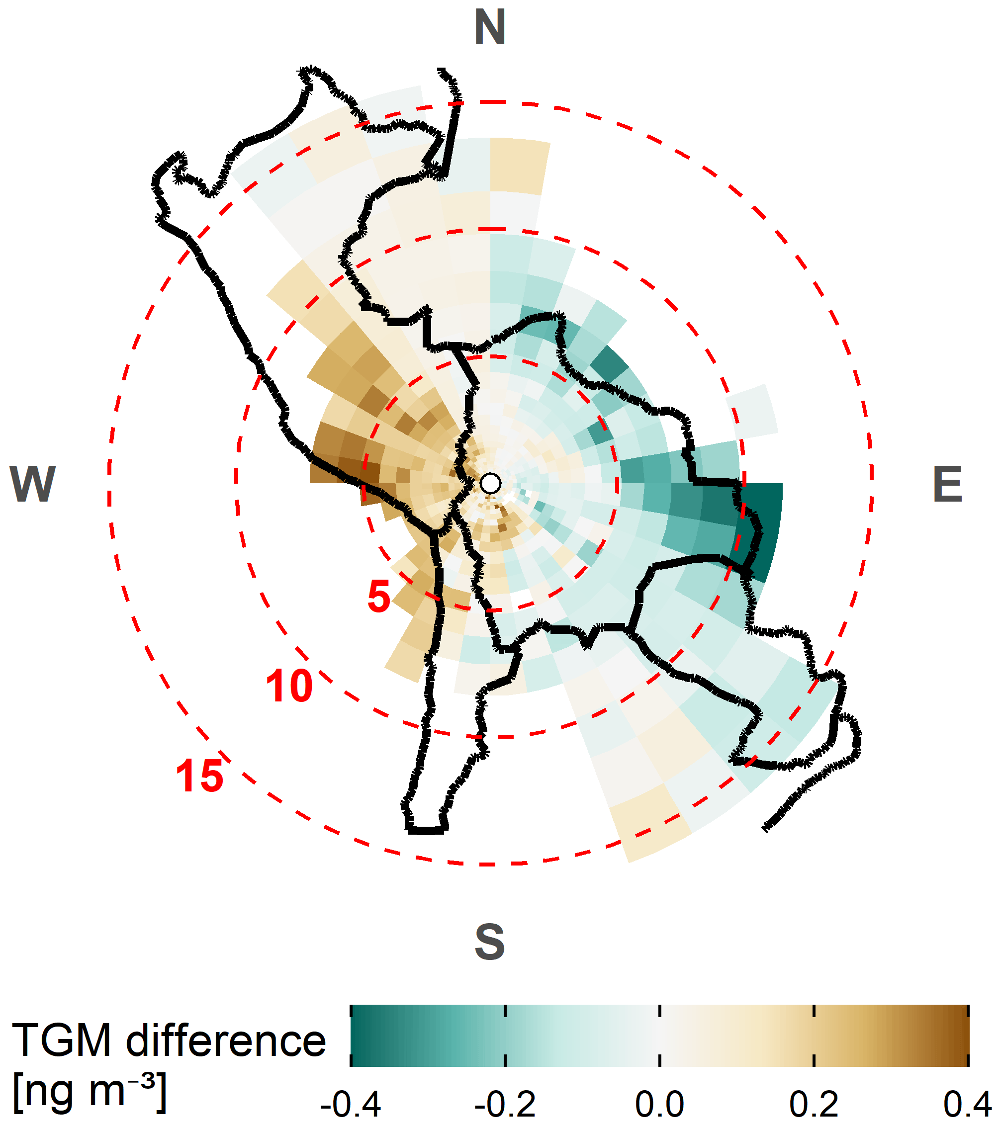
Figure 9 Pollution map for the wet season (austral summer) minus pollution map for the rest of the NC period. The polar grid is centered on CHC (white dot). Dashed range circles show the distance to CHC in degrees, which can be converted to kilometers using the conversion factor 1^∘ = 108.6 km, with an error below 3 % in the whole domain. Trajectory endpoints with an elevation >1000 m a.g.l. and cells with less than 10 data points (n<10) were excluded. The color scale was capped at the limits.

Thus, we hypothesize that changing emission patterns over the eastern Pacific Ocean might play a role in the seasonal pattern of atmospheric mercury in the Bolivian Andes. Increased Hg emissions during the wet season (austral summer) might be linked to an increase in SST and/or the southwards shift of the ITCZ and enhanced convection over the southern Pacific Ocean.

4.5 Volcanic influences

Previous studies have reported volcanic degassing in the CVZ, both south of CHC (Tamburello et al., 2014; Tassi et al., 2011) and west of CHC (Moussallam et al., 2017). While, to our knowledge, mercury emissions or atmospheric mercury concentrations have not yet been investigated in the CVZ, a very recent work inferred, from mercury concentrations in lichen, that volcanoes in the Southern Volcanic Zone (south of the CVZ) can be sources of atmospheric mercury (Perez Catán et al., 2020). As similar gas plume compositions (${\mathrm{CO}}_{\mathrm{2}}/S_{\mathrm{TOT}}$, $S_{\mathrm{TOT}}/\mathrm{HCl}$) were measured in volcanic emissions from the CVZ and the Southern Volcanic Zone (Tamburello et al., 2014), we can hypothesize that volcanoes in both active regions emit mercury in a similar fashion.

That being said, our data give ambivalent information about the importance of a volcanic Hg source in the region.

On the one hand, we found elevated mean TGM concentrations of above 1.08 ng m⁻³ (± 0.08 ng m⁻³) in air masses passing at low altitudes (under 1000 m a.g.l.) over the southwestern frontier between Bolivia and Chile, the same regions of the CVZ where Tassi et al. (2011) and Tamburello et al. (2014) reported important volcanic degassing (Fig. 6a). Southern Altiplanic cluster C3 in comparison, which best represents the general origin of similar air masses, showed mean TGM concentrations only insignificantly higher than the NCs as a whole (0.92±0.04 ng m⁻³ vs. 0.89±0.01 ng m⁻³, p=0.067, Mann–Whitney test). Admittedly, special care has to be taken with air masses of this general direction, as they frequently move over the La Paz–El Alto urban area (Chauvigné et al., 2019) before arriving at CHC and could be occasionally enriched in Hg, even though the city does not generally seem to play an important role in average Hg concentrations (see the TGM diel pattern; Fig. 4a). We evaluated this possibility by excluding data with high eBC concentrations (>87.5th eBC percentile of NCs), which are apparently strongly linked to urban pollution (Fig. 4c; Wiedensohler et al., 2018), without an apparent change in the above results. Therefore, these elevated TGM concentrations in air masses passing over degassing volcanoes to the south of CHC are unlikely to be caused by urban pollution on the way and might indeed be related to volcanic emissions.

On the other hand, TGM concentrations in air masses passing over the Ubinas and Sabancaya volcanoes to the west of CHC did not appear to be significantly elevated, compared with air masses of similar origin (pollution map, Fig. 6a), even though both volcanoes are currently strongly degassing and together account for more than half of the entire CVZ volatile fluxes, as estimated by Moussallam et al. (2017). They also lie in a frequent source region for air masses arriving at CHC, especially in the dry season (Fig. 5).

Thus, our data provide an inconclusive picture of the role of the CVZ in the atmospheric mercury budget in the region. While a volcanic mercury source south of CHC can be supported due to significantly elevated TGM concentrations in the source region, we cannot say the same for volcanoes to the west of CHC, even though both Ubinas and Sabancaya were strongly emitting other volcanic gases such as SO₂ during the NC period (Carn et al., 2017; Moussallam et al., 2017). This inconsistency might be related to the complexity of volcanic mercury emissions, whose quantity is highly variable between different volcanoes, their activity phase, and different points in time (Bagnato et al., 2011; Ferrara et al., 2000). For instance, volcanic Hg $/$ SO₂ emission ratios obtained in the literature span several orders of magnitude (Bagnato et al., 2015). Moreover, given that our setup does not detect mercury in particulate form, the magnitude of any volcanic signal received at CHC also depends on the mercury gas–particle partitioning at the time of emission, as well as the transformations it undergoes during the transport.

4.6 Artisanal and small-scale gold mining (ASGM)

ASGM is known to be a major source of mercury pollution and is especially important in Latin America (Esdaile and Chalker, 2018; Obrist et al., 2018). According to recent inventories, South America contributes 18 % of global Hg emissions to the atmosphere, with 80 % of it deriving from the ASGM sector (UNEP GMA 2018). One prominent ASGM hot spot on the continent is the Madre de Dios watershed, a few hundred kilometers north of CHC station (Fig. 1), where high Hg concentrations have been found among others in sediments and human hair (Langeland et al., 2017; Martinez et al., 2018).

As shown in Fig. 6b, we measured the highest TGM concentrations in northern Amazonian air masses (cluster C1), which pass mostly over the Madre de Dios watershed. Notably, C1 air masses in the wet season showed much higher mean Hg concentrations than the other important lowland cluster C2, which does not pass over this region (0.91±0.02 ng m⁻³ vs. 0.82±0.02 ng m⁻³, $p=\mathrm{9.9}\times {\mathrm{10}}^{-\mathrm{12}}$, Mann–Whitney test). Still, TGM is uniformly high for most of the north and northeastern lowland air masses, and the Madre de Dios region does not actually appear distinctively in our pollution maps (Fig. 6a). This could be explained by ASGM being scattered rather evenly around a large part of the Bolivian lowlands, instead of being clustered around a few hot spots. This is certainly not an unlikely scenario, but it has to be acknowledged that the techniques applied here might not provide the necessary resolution to clearly discern isolated ASGM hot spots hundreds of kilometers away, given dilution and diffusion processes and the uncertainties in HYSPLIT trajectories.

5 Conclusions

Our measurements of TGM at the CHC mountain site fill an important gap in observations for South America and allow us to make justified assumptions about the dynamics of atmospheric mercury on the continent.

During the NC period, mean TGM concentrations at CHC were relatively low compared with other sites in the Southern Hemisphere, but similar to those in South America. However, we detected a significant rise of atmospheric Hg levels during ECs, which might well be related to the 2015–2016 El Niño, which is a hypothesis we will address in an upcoming publication. In the regional overview, mercury concentrations were higher in air masses with northern Amazonian or southern Altiplanic origin, with the former possibly related to a strong ASGM presence in the source region, whereas the latter might be of volcanic origin. In agreement with other South American sites but in contrast with different regions in the Southern Hemisphere, we observed a marked seasonal pattern. Concentrations were lowest in the dry season (austral winter), rising in the BB season, and highest at the beginning of the wet season (austral summer). To explain this, we explored several possible drivers for this seasonal cycle. BB-related Hg emissions appear to significantly raise atmospheric Hg levels during a limited time of the year, mainly between August and October (BB season). Vegetation on the continent, most prominently the Amazon rainforest, seems to act as an important mercury sink, at least during months of high gross primary production (around February–April). The former allowed us to deduce a TGM $/$ CO emission ratio of $(\mathrm{2.3}\pm \mathrm{0.6})\times {\mathrm{10}}^{-\mathrm{7}}$ ppbv_TGM ppbv${}_{\mathrm{CO}}^{-\mathrm{1}}$, while we used the latter to infer a best guess TGM $/$ CO₂ uptake ratio of 0.058±0.017 (ng m⁻³)_TGM ppm${}_{{\mathrm{CO}}_{\mathrm{2}}}^{-\mathrm{1}}$. Finally, arguments can be made for a significant influence of the eastern Pacific Ocean on regional Hg levels, possibly through a shift in ocean–atmosphere Hg exchanges in response to rising sea surface temperature and deep convection in austral summer.

Notably, all three of these major regional drivers of atmospheric mercury might undergo significant changes in the near future. On the one hand, Pacific SST and convection dynamics could shift as a consequence of climate change. On the other hand, both upcoming BB emissions and the magnitude of the South American vegetation sink will depend heavily on the future of the Amazon rainforest, which itself is threatened by climate change and changes in land use, such as deforestation and agricultural practices. In perspective, the TGM $/$ CO emission ratio and TGM $/$ CO₂ uptake ratio obtained here could be used to constrain both current and future South American biomass burning Hg emissions and vegetation Hg uptake, with the help of remotely sensed CO and CO₂ data products and model results.

Appendix A: Seasonality of CO concentrations in South America and CHC

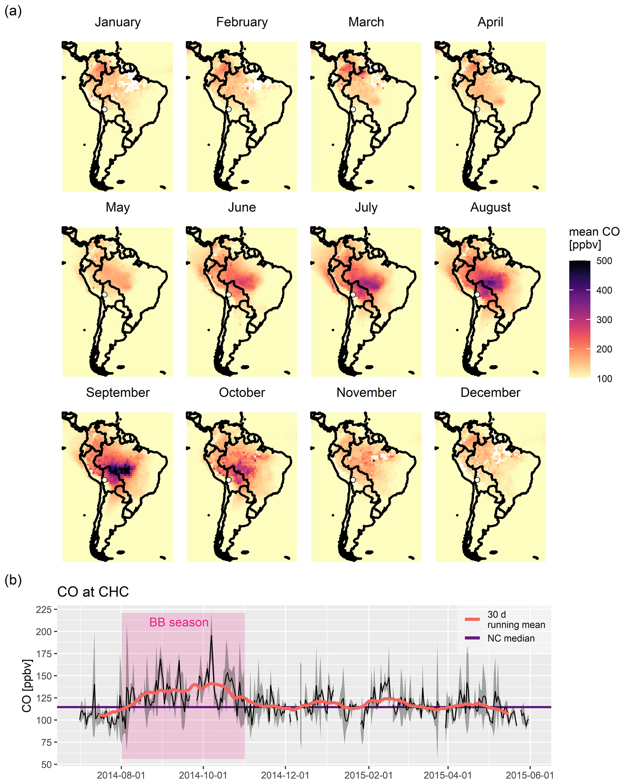
Figure A1 (a) Seasonality of remotely sensed tropospheric CO concentrations in South America from January 2005 to January 2015, based on the MOP03J_V008 data product (Ziskin, 2019). The white dot shows the CHC station. (b) Daily mean CO concentrations at CHC under “normal conditions” (NCs; 1 July 2014 until 1 June 2015). The gray shaded area shows the standard deviation, the orange line shows the 30 d running mean, and the purple line shows the NC median. The pink box illustrates the definition of the biomass burning (BB) season used in the present work.

Appendix B: Pollution maps at different cutoff altitudes

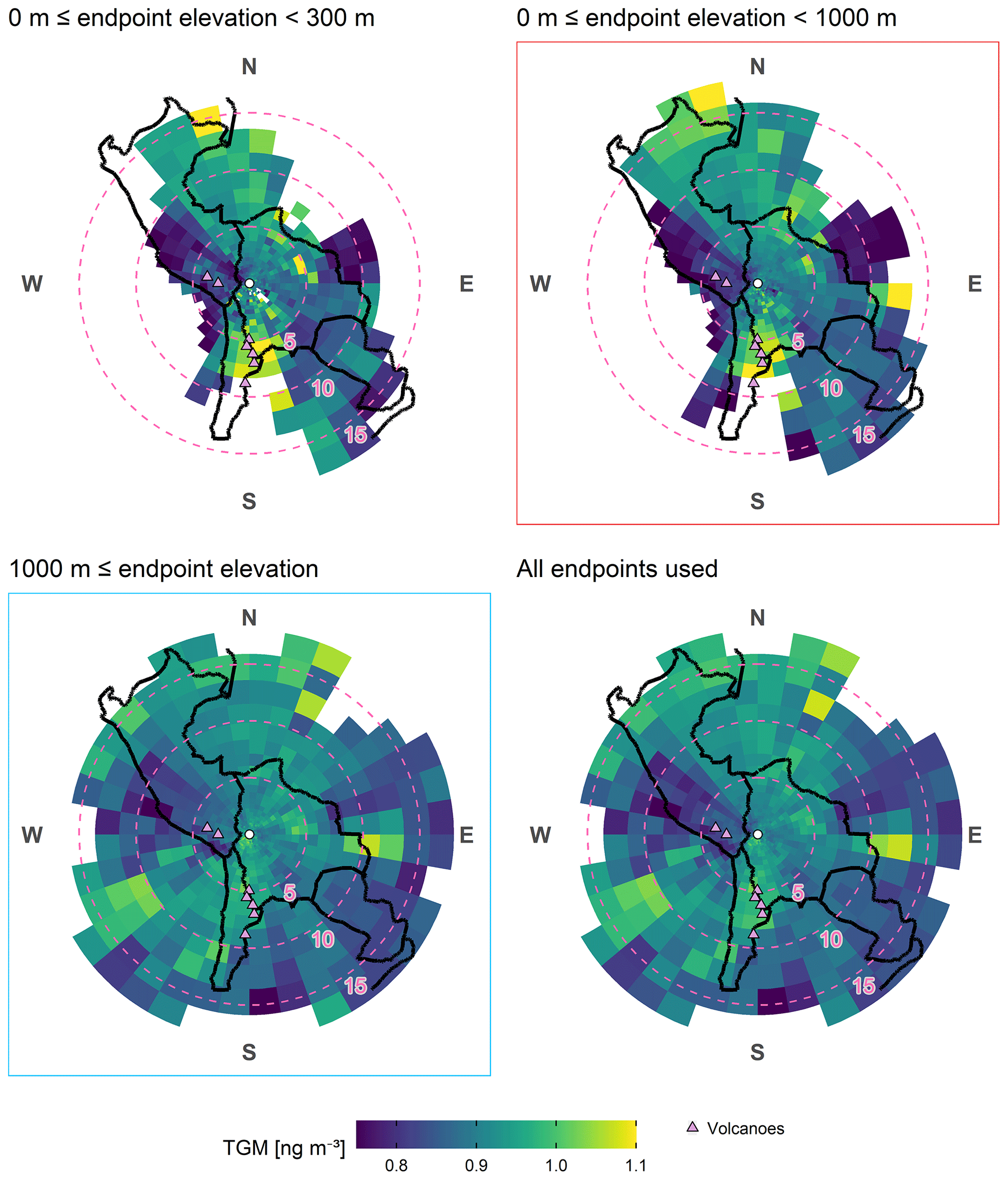
Figure B1 Pollution maps based on all TGM data taken during NCs, calculated using the different cutoff altitudes specified by the panel titles. The plot corresponding to the cutoff altitude used in the main text (endpoint elevation <1000 m a.g.l.) is framed in red. The plot based on all endpoints that were excluded from the pollution map shown in the main text is framed in blue. Dashed range circles show the distance to CHC in degrees, which can be converted to kilometers using the conversion factor 1^∘ = 108.6 km, with an error below 3 % in the whole domain. The color scale is capped at the limits. Cells with less than 10 data points (n<10) were excluded. Pink triangles show selected degassing volcanoes in the CVZ : Sabancaya, Ubinas, Ollagüe, San Pedro, Putana, Lascar, and Lastarria (from north to south).

Appendix C: Median transport time for HYSPLIT back trajectories arriving at CHC

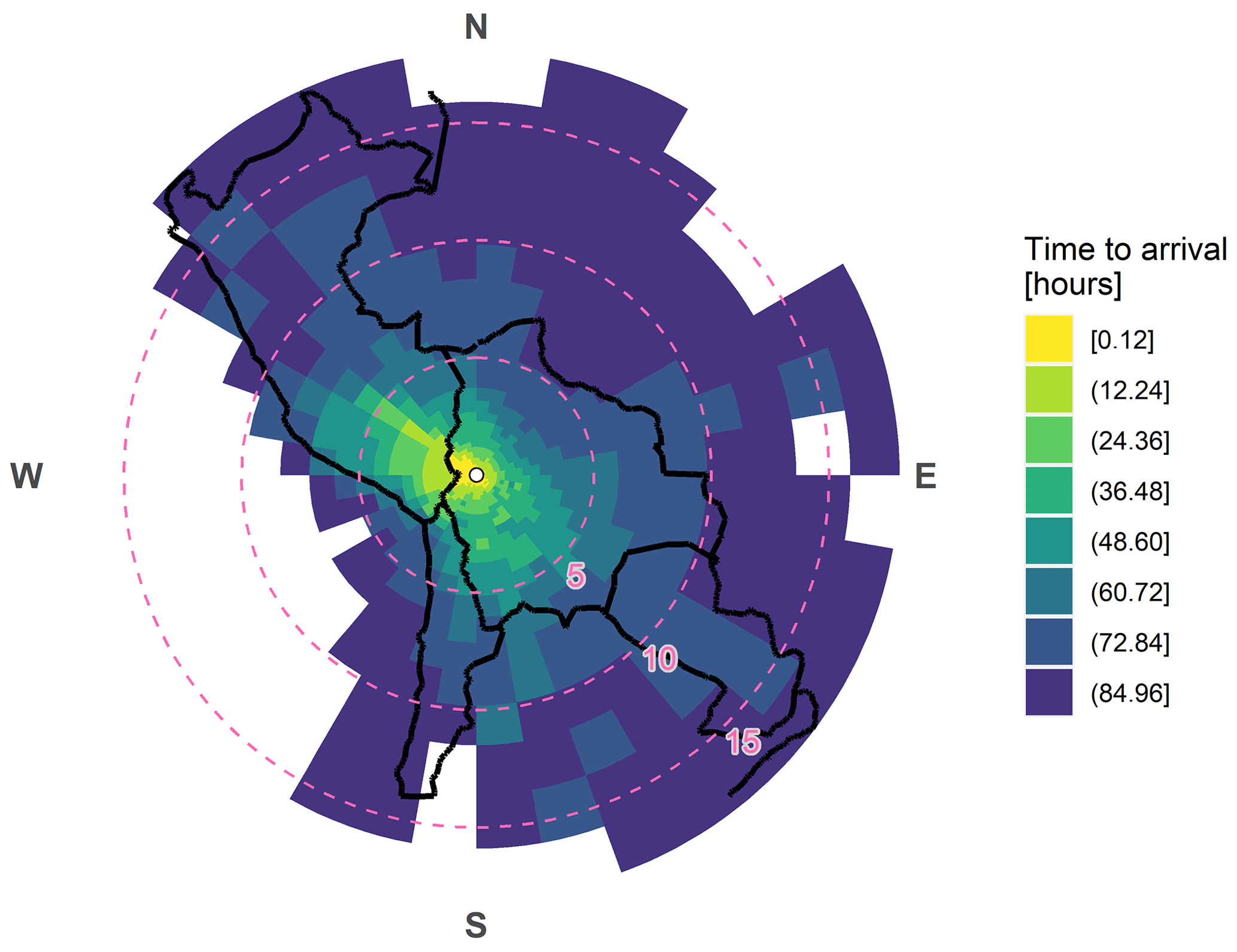
Figure C1 Average transport time between the air mass source region and CHC, shown through the median time passed between HYSPLIT trajectory pixel piercing and arrival at CHC. Dashed range circles show the distance to CHC in degrees, which can be converted to kilometers using the conversion factor 1^∘ = 108.6 km, with an error below 3 % in the whole domain. The figure is based on all trajectories during NCs (1 July 2014–1 June 2015) and endpoints with an elevation below 1000 m a.g.l.

Appendix D: Sensitivity analysis for the calculation of the TGM $/$ CO emission ratio

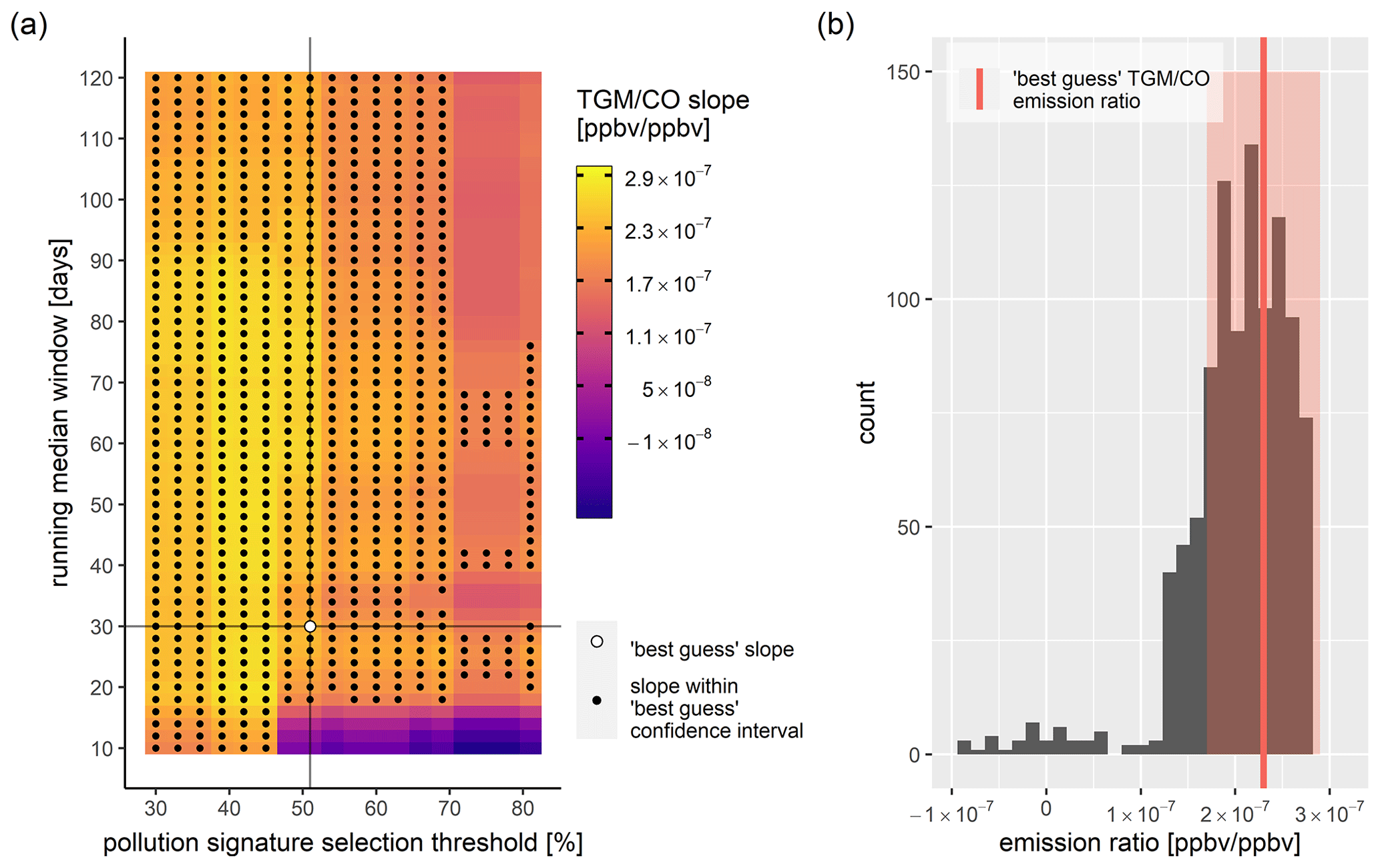
Figure D1 Sensitivity analysis for the calculation of the TGM $/$ CO emission ratio as a function of the chosen threshold for the selection of biomass burning pollution signatures (percentage of time the pollution signature fell into the BB season) and the choice of the size of the “running window” (in days) to calculate the median TGM background concentrations. (a) Heat map showing the obtained TGM $/$ CO emission ratios for a wide range of combinations of the pollution signature threshold (x axis) and the running window (y axis). The best guess TGM $/$ CO emission ratio, as presented in the main text, is marked as a white dot, and black dots show all combinations for which the calculated slope is within the best guess confidence interval. (b) Histogram for all TGM $/$ CO slopes shown in panel (a) (the heat map). The best guess emission ratio and its confidence interval are shown in red.