the Creative Commons Attribution 4.0 License.
the Creative Commons Attribution 4.0 License.
 | 20 Oct 2021
Technical note: Quality assessment of ozone reanalysis products and gap-filling over subarctic Europe for vegetation risk mapping
Stefanie Falk
Ane V. Vollsnes
Aud B. Eriksen
Frode Stordal
Terje Koren Berntsen
We assess the quality of regional and global ozone reanalysis data for vegetation modeling and ozone (O3) risk mapping over subarctic Europe where monitoring is sparse. Reanalysis data can be subject to systematic errors originating from, for example, quality of assimilated data, distribution and strength of precursor sources, incomprehensive atmospheric chemistry or land–atmosphere exchange, and spatiotemporal resolution. Here, we evaluate two selected global products and one regional ozone reanalysis product. Our analysis suggests that global reanalysis products do not reproduce observed ground-level ozone well in the subarctic region. Only the Copernicus Atmosphere Monitoring Service Regional Air Quality (CAMSRAQ) reanalysis ensemble sufficiently captures the observed seasonal cycle. We also compute the root mean square error (RMSE) by season. The RMSE variation between (2.6–6.6) ppb suggests inherent challenges even for the best reanalysis product (CAMSRAQ). O3 concentrations in the subarctic region are systematically underestimated by (2–6) ppb compared to the ground-level background ozone concentrations derived from observations. Spatial patterns indicate a systematical underestimation of ozone abundance by the global reanalysis products on the west coast of northern Fennoscandia. Furthermore, we explore the suitability of CAMSRAQ for gap-filling at one site in northern Norway with a long-term record but not belonging to the observational network. We devise a reconstruction method based on Reynolds decomposition and adhere to recommendations by the United Nations Economic Commission for Europe (UNECE) Long-Range Transboundary Air Pollution (LRTAP) convention. The thus reconstructed data for 2 weeks in July 2018 are compared with CAMSRAQ evaluated at the nearest-neighbor grid point. Our reconstruction method's performance (76 % accuracy) is comparable with CAMSRAQ (80 % accuracy), but diurnal extremes are underestimated by both.
- Article
(7931 KB) - Full-text XML
- BibTeX
- EndNote


Tropospheric ozone (O3) as a secondary pollutant is highly toxic and harmful to human health (WHO – World Health Organization, 2008; Fleming et al., 2018) and a variety of ecosystems globally (Mills et al., 2011, 2018; Emberson, 2020). At the same time O3 acts as a potent greenhouse gas (Myhre et al., 2013). Ozone causes an estimated annual global yield loss of four major crops (wheat, rice, maize, and soybean) of 3 %–15 % (Ainsworth, 2017) and threatens food security in rapidly developing countries, e.g., in East Asia and Southeast Asia (Tang et al., 2013; Tai et al., 2014; Chuwah et al., 2015; Mills et al., 2018).
In the troposphere, O3 is produced in complex chemical cycles involving precursors such as carbon monoxide (CO) and hydrocarbons (e.g., methane, terpenes) in the presence of nitrogen oxides (NOx) (Monks et al., 2015). These hydrocarbons can be of anthropogenic or natural origin and are often referred to as volatile organic compounds (VOCs) and biogenic VOCs (BVOCs), respectively. The primary sink of O3 in the troposphere is dry deposition to different surfaces of which the removal by vegetation amounts to over 50 % (Monks et al., 2015; Clifton et al., 2020). Plants take up O3 through their stomata (leaf openings for gas exchange). In the leaf interior, O3-induced radical oxygen species (ROS) damage cell membranes, leading to necrosis and ultimately to programmed cell death (Kangaskärvi et al., 2005). Ozone damage is considered to accumulate over time. To assess the potential risk posed by ozone, various metrics have been defined. Mills et al. (2011) showed that the phytotoxic ozone dose over a threshold y (PODy) (integrated flux through the stomata) is capable of capturing observed negative effects on crops and seminatural vegetation (e.g., clover) better than an integrated exceedance over a fixed threshold (e.g., 40 ppb). Furthermore, O3 uptake and subsequent damage negatively affect photosynthesis and stomatal conductance (e.g., Pellegrini et al., 2011; Watanabe et al., 2014). This, in turn, reduces gross primary production (GPP) (Lombardozzi et al., 2015b, a; Hoshika et al., 2015) and has the potential to off-set growth effects of carbon dioxide (CO2) fertilization in the future (Franz and Zaehle, 2021) as well as to induce measurable positive feedback on surface temperatures in highly polluted regions (Zhu et al., 2021).
Due to these risks, O3 is included in air quality monitoring networks under the WMO (World Meteorological Organization) Global Atmosphere Watch (GAW) program. Remote regions in the Arctic and subarctic, however, are scarcely covered (refer to Sect. 2 for the coverage of northern Fennoscandia). With climate change already promoting an earlier and longer growing season (Linderholm, 2006; Karlsen et al., 2007; Høgda et al., 2013), subarctic vegetation may become more vulnerable to damage induced by cumulative O3 uptake in the future. Although, species acclimated to the Arctic and subarctic climates were not found to be more sensitive to ozone than species in less extreme environments (Karlsson et al., 2021).
O3 as well as its precursors is subject to atmospheric transport, causing pollution peaks in the otherwise pristine Arctic and subarctic environments (Stevenson et al., 2005; Young et al., 2013). This long-range transport of pollutants has been identified as one of the main sources of enhanced O3 concentration ([O3]) in Fennoscandia (Andersson et al., 2017). Here, [O3] refers to the concentration as volume mixing ratio (VMR) of ozone in ppb. Peak [O3] in summer is often a combination of stagnant weather situations accompanied by heat waves and enhanced precursor emissions due to extensive forest fires (e.g., in 2003, 2006, 2018) (Lindskog et al., 2007; Karlsson et al., 2013). The prominently elevated [O3] which occurs in April–May over northern Fennoscandia is caused by other factors. This so-called ozone spring peak can be attributed to a build-up of O3 and precursors due to a suppression of removal from the troposphere during the polar night and their photo-chemical reactivation come spring (Monks, 2000). Tropopause folding events are another contributor and cause an intrusion of dry and O3-rich air masses from the stratosphere (Škerlak et al., 2015).
As indicated above, PODy is an integrated O3-flux quantity. A proper assessment of PODy relies on a set of complete, 1-hourly meteorological and ozone data. Since gaps in observational data are common, many techniques of varying complexity have been devised for filling these. The applicability often depends on the shape of the variables' signal, e.g., prominence of the diurnal cycle. In the simplest case of monotonically increasing/decreasing data and little fluctuation, a first-order polynomial may suffice. In the following, we give an account of the detailed practical recommendations by Mills et al. (2020). For gaps of less than 5 h, gap-filling with an average value over the preceding and subsequent time steps is recommended. This method, however, does not suffice for observables such as O3 that display a distinct diurnal cycle and leads to an underestimation around noon and an overestimation during the night. Similarly, gaps longer than 5 h but less than 24 h ought to be filled by averaging the preceding and subsequent day at each time step. For gaps exceeding 1 d, Mills et al. (2020) suggest exploiting data from close-by monitoring stations with a Pearson correlation coefficient r2 of preferably 0.6 or higher. A period of at least one season (3 months) is recommended for this statistical analysis. To account for the seasonal variability, the projection between sites is to be computed for the same season the gap occurred. Where available, auxiliary data from model reanalysis can be used.
As indicated above, reanalysis data can be used for gap-filling, but more often they are used to study emerging trends in tropospheric ozone in remote regions such as the Arctic and subarctic, where scarce observations have to be supplemented with model simulations. Atmospheric reanalyses are based on a fixed state of an operational data assimilation system used for forecasts ingested with the most complete set of observational data. In terms of atmospheric chemistry, this includes meteorological data as well as observations of chemical substances from, for example, satellite, airborne instruments, and ground-level monitoring station networks. Global reanalyses, however, have already been shown to underestimate [O3] particularly over the polar region (Huijnen et al., 2020; Barten et al., 2021). Barten et al. (2021) suggest that global reanalysis products that only assimilate satellite products do not sufficiently cover [O3] variations. The large discrepancies can be explained by the low spatiotemporal resolution not capturing atmospheric boundary layer dynamics and missing processes such as mechanistic ocean–atmosphere O3 exchange.
In the following, we evaluate and validate the quality of three reanalysis products concerning surface ozone over northern Fennoscandia with available long-term observations. All data are presented in Sect. 2. In Sect. 3, we derive a generalized ozone climatology for northern Fennoscandia from in situ observations and quantify the overall quality of the ozone reanalysis. We look at the respective seasonal cycles and spatial patterns, and we derive the relative impact on an integrated-flux metric. Based on these results, we provide a methodology for reconstructing missing observational data over an extended period of several weeks based on Reynolds decomposition and compare it with the evaluation of the best reanalysis product at the nearest-neighbor grid point. We close with discussions and conclusions (Sect. 4).
In this section, we present long-term ground-level O3 observation data for our focus area, northern Fennoscandia, which we define here as north of 67.5∘ N, and we determine their correlation. To this end, we compute Pearson correlation coefficients pairwise. All observational data are taken from the EBAS atmospheric database (NILU, 2020) operated by the Norwegian Institute for Air Research (NILU). We also present the selected ozone reanalysis products provided by the European Centre for Medium-Range Weather Forecasts (ECMWF) and the Copernicus Atmospheric Monitoring Service (CAMS).
2.1 Ozone monitoring sites
Northern Fennoscandia is sparsely covered by sites that monitor ground-level background [O3] and report to the EBAS atmospheric database (Fig. 1). A detailed overview over the past and present ozone monitoring sites in northern Fennoscandia with a considerable duration of data acquisition is given in Table 1. Continuous ozone data are available as early as mid-1986 from the NILU atmospheric monitoring site at Svanvik located in the Pasvik valley. Measurements, however, did not continue after 1996. To supplement field experiments on subarctic vegetation, we installed an ozone monitor at Svanvik exclusively for the growing seasons 2018/19 in collaboration with NILU. Due to irregularities in data acquisition, 2 weeks of data are missing from the record in July 2018. These shall be subject to our proposed data reconstruction (Sect. 3.3). At the same latitude but further west, a station was established in the early 1990s above the Karasjohka river valley. Originally placed at Jergul, the station was later moved downstream closer to the city of Karasjok using the same equipment but increasing the recorded floating-point precision of the ozone monitor. The station was decommissioned in 2011. Data series from Svanvik and Jergul are highly uncertain because of insufficient quality control and irregular calibration before 1997, which led to degradation of the monitors over time and introduced drifts in the ozone data series (Solberg, 2003). Solberg (2003) further reported a systematic uncertainty for these data on the order of 10 %, which they deemed too large to conduct a strict trend analysis of ground-level background [O3]. For our purpose of evaluating seasonal cycles on a climatological timescale, we can consider these uncertainties as small enough. Further south, two stations have been established at Esrange (Sweden) and Pallas (Finland) in the early 1990s. Data are available from EBAS until the end of 2018 and 2019, respectively (last accessed April 2021).
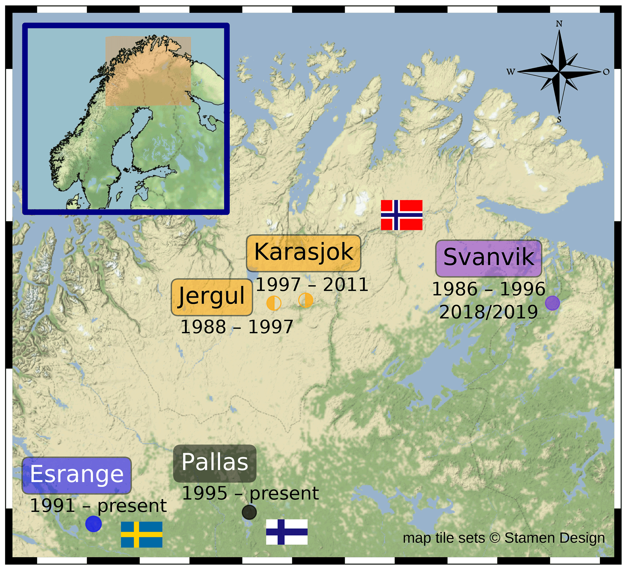
Figure 1Subarctic Europe north of 67.5∘ N, here referred to as northern Fennoscandia. Locations of past and present ozone observation sites used in this study. For more details, see Table 1. The introduced color coding for the monitoring sites is used throughout.
Table 1Past and present ozone observation sites in northern Fennoscandia. Data are available from http://ebas.nilu.no/ (last access: April 2021).
a Data availability on EBAS at present.
b Exclusive monitoring in growing season 2018/19.
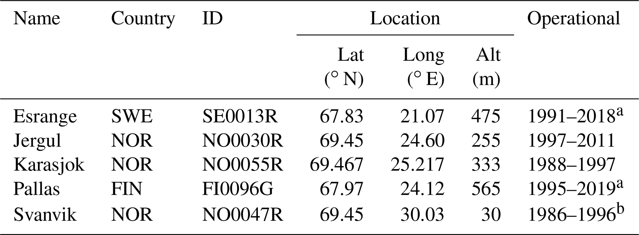
In Fig. 2, daily mean ozone concentration climatologies (〈[O3]〉) for the data taken at Esrange, Jergul/Karasjok, Pallas, and Svanvik are shown together with their respective standard error (). The annual average 〈[O3]〉 at Svanvik is 6.6 ppb lower compared to the other sites. This can be attributed to the station's location at lower altitude and amidst agriculturally used land surrounded by forests in contrast to Pallas where the vegetation consists of low vascular plants, mosses, and lichen (Hatakka et al., 2003). An increase in ground-level background [O3] since the early 1990s cannot be dismissed. Given 2019 was a climatologically normal year, we estimate the deviation from the 1990s ozone climatology at Svanvik as ppb. The δ[O3] indicates a small and statistically insignificant increase in [O3].
The Pearson correlation coefficients (r2) for the combined data set of Jergul/Karasjok show a high correlation with Esrange (r2=0.78) as well as Pallas (r2=0.79). We, therefore, combine observational data from Esrange, Jergul/Karasjok, and Pallas to derive a generalized ozone climatology for northern Fennoscandia which represents the expected ground-level background in this region. The correlation of Svanvik with Esrange is fair (r2=0.42) but good with Pallas (r2=0.61). The climatologies displayed in Fig. 2 cover the known features of the ozone seasonal cycle in northern Fennoscandia well and reflect the expected increase of ozone abundance with altitude where Pallas is located at the highest altitude and Svanvik at the lowest. The highest average ozone concentration ( ppb) is regularly observed in April–May and the lowest average concentration is reached in August–September ( ppb). The values lie well below 0.5 ppb for Esrange, Jergul/Karasjok, and Pallas. This is considerably lower than at Svanvik ( ppb) and can be attributed to the length of these time series, a better quality control, and less diurnal variability at higher altitudes.
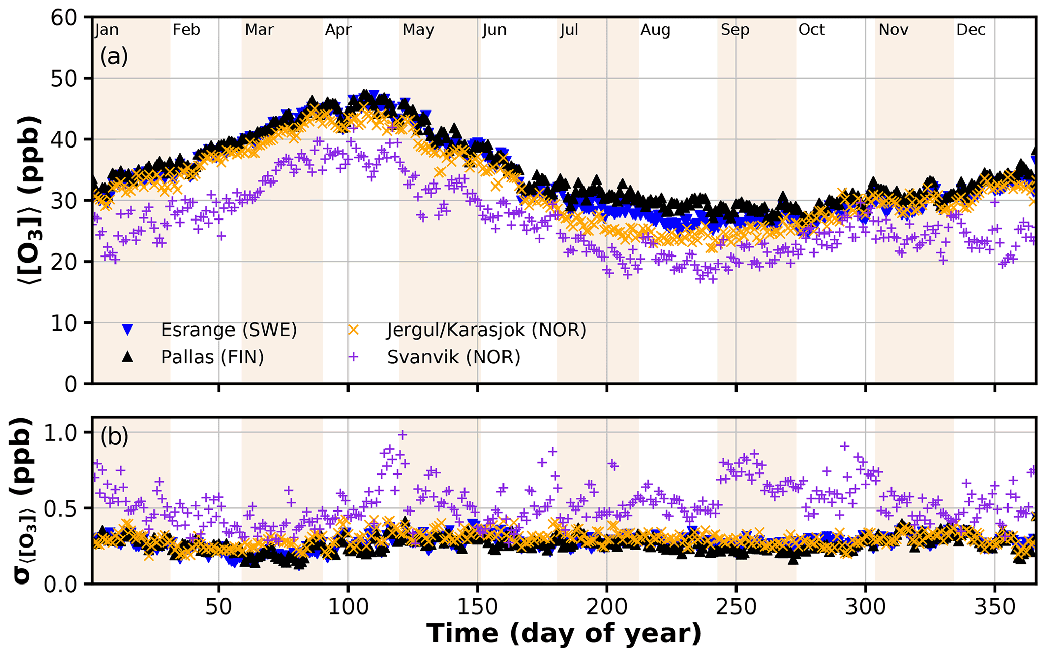
Figure 2Daily mean ozone climatologies (upper panel) and standard error (lower panel) over the day of the year. All stations located in northern Fennoscandia with data records exceeding 10 years are displayed. The data taken at Jergul and Karasjok have been combined.
2.2 Ozone reanalysis
From the global reanalysis products available from ECMWF that include atmospheric tracers, including ozone, we select the Monitoring Atmospheric Composition and Climate (MACC) and the latest Copernicus Atmosphere Monitoring Service reanalysis (CAMSRA) (Inness et al., 2013, 2019). The temporal and spatial resolutions of these reanalysis products are rather coarse: 3-hourly and or roughly 29.3 km×83.4km at the location of Svanvik. From the Copernicus Atmospheric Monitoring Service Regional Air Quality (Copernicus Atmosphere Monitoring Service, 2020b) system, surface ozone reanalysis ensemble means are available for a European domain. CAMSRAQ is based on nine European state-of-the-art numerical air quality models. The ensemble mean is at higher spatial and temporal resolution compared to the global reanalyses: (roughly 3.9 km×11.1 km at Svanvik) and 1-hourly. The periods covered differ but no data are available before the turn of the millennium. CAMSRA is available in near real time and covers a period of sufficient length for climate analysis (2003–present). For this study, a shorter subset of CAMSRA (2003–2012) has been chosen for comparability with the MACC reanalysis in terms of statistical uncertainties. Predominately, the CAMSRAQ system is used for air quality forecasting and the reanalysis has currently not been extended beyond 2018.
All reanalysis products apply the latest version of the operational weather forecast system (OpenIFS) of ECMWF to force their models. Concerning the assimilated observational ozone data, all reanalysis products differ. The MACC reanalysis assimilates only satellite-derived tropospheric column ozone, while CAMSRA also includes ozone profiles from satellite retrievals. In situ observations from ozone near-surface station networks are only assimilated in the CAMSRAQ reanalysis ensemble. All relevant details concerning the reanalysis data sets are listed in Table 2.
Table 2Global/regional ozone reanalysis products used in this study.

a Layer thickness at ground level, same as for operational IFS. b Subset of reanalysis data used in this study. c ERA5 (2003–2016), OPS (later). d EURAD uses WRF for downscaling of operational IFS. e MLS, OMI – tropospheric column. f SCIAMACHY, MIPAS, MLS, OMI, GOME2, SBUV2 – tropospheric column + profile. g Météo-France NRT.
The MACC reanalysis is still well known and used in the wider community, albeit with lower accuracy compared to CAMSRA (Huijnen et al., 2020). To assess whether and how the improvements to the CAMS assimilation system affect the reanalysis results in our focus area, we analyze both MACC and CAMSRA. CAMSRAQ has been specifically chosen to test whether a higher spatiotemporal resolution will also give better results in our focus area.
On global scales, at least two other ozone reanalysis products are available: the Tropospheric Chemistry Reanalysis (TCR) 1 and 2 (Miyazaki et al., 2020) and the Japanese Reanalysis 55 (JRA-55) (Kobayashi et al., 2015). As part of the comprehensive reanalysis intercomparison study by Huijnen et al. (2020), TCR-1 and TCR-2, CAMS interim reanalysis, and CAMSRA were used by means of seasonal averages. The results suggested a similar performance of CAMSRA and TCR-2 in our focus area. Therefore, we assume our selection to be representative of the state-of-the-art global reanalysis products.
The comprehensive JRA-55 reanalysis is the longest reanalysis data set available spanning several decades. With a horizontal resolution of T319, 6-hourly temporal resolution, and interpolation to pressure levels (e.g., 1000 hPa), it is too coarse and not suitable for our purpose.
In the following, we assess the quality of the reanalysis products, MACC, CAMSRA, and CAMSRAQ, with respect to the generalized ozone climatology derived from ground-level ozone observations in northern Fennoscandia. We focus in particular on the seasonal cycle of [O3] with its prominent peak in spring and dip in late summer and identify the reanalysis product that best reproduces these features. Concerning ozone risk mapping, we assess implications on an integrated-flux metric that is similar to PODy. We then devise a reconstruction method for missing data applicable for extended periods of data gaps based on Reynolds decomposition and compare with the best reanalysis product evaluated at the nearest-neighbor grid point of Svanvik.
3.1 Quality of ozone reanalysis products in northern Fennoscandia
First, we evaluate the reanalysis products qualitatively at the site level. We compare the seasonal cycle of the generalized ozone climatology with seasonal cycles derived for each reanalysis product at the nearest-neighbor grid point of the actual monitoring sites. In this way, we can also test the vertical resolution of the products concerning the expected ozone abundance in response to differing ground-level altitudes.
The generalized ozone climatology and its respective standard deviation (gray band) shown in Fig. 3 are based on a spline fitted through the climatological daily mean [O3]. The global products (MACC, CAMSRA) do not reproduce the observed seasonality of ground-level [O3] well. The MACC reanalysis (Fig. 3a) reveals a strong negative deviation (bias) amounting to ppb on average and displays no distinct seasonal cycle. The ozone climatology is rather flat throughout the whole cycle with a small peak in March. MACC [O3] is considerably too low compared to the generalized climatology in all seasons but summer. The March peak is followed by a flattening and a second peak in July. The seasonal low is shifted towards November–December.
CAMSRA matches the observed ozone climatology poorly (Fig. 3b). Despite reproducing [O3] well during the growing season (May–October), it does not reproduce the actual seasonality in northern Fennoscandia. The CAMSRA-derived spring peak lags behind observations by 1 month and is 5 ppb too low, whereas the minimum occurs in January compared to August–September. In general, CAMSRA fails in reproducing [O3] in all seasons but summer. The annual amplitude ((26±1) ppb) is larger than in the climatology derived from observations (19 ppb). Both global reanalysis products place the O3 abundance evaluated at the location of Svanvik highest. This indicates an insufficient vertical resolution of these models. This is important in terms of usage for gap-filling as well as Europe-wide or global risk assessment concerning the Arctic and subarctic vegetation that may rely on these data.
In contrast, the ensemble mean of CAMSRAQ reproduces the seasonal cycle in northern Fennoscandia well (Fig. 3c). CAMSRAQ correctly depicts [O3] at Svanvik lower than at the other sites most likely due to the higher resolution and data assimilation of in situ ozone observation. On average, CAMSRAQ slightly underestimates [O3] ( ppb) compared to observations.
However, the reanalysis products' time series are not sufficiently long enough to study deviations from the observed climatology with a high statistical significance. However, the associated standard deviation is usually smaller in models compared to observations due to the inherent spatiotemporal averaging. This has no impact on our qualitative results. Recent analyses indicate a leveling or decline of tropospheric background [O3] over Europe after 2007 (Cooper et al., 2014; Wespes et al., 2018; Gaudel et al., 2018), following a steady increase over the past decades (Hartmann et al., 2013, Chapter 2). This indicates that the observation-based generalized northern Fennoscandia climatology which includes data before 2007 could be biased towards a higher annual average [O3]. As estimated in Sect. 2.1, the climatology derived for Svanvik is insignificantly underestimating present-day [O3].

Figure 3Daily mean ozone climatologies computed from the ozone reanalysis products (a) MACC, (b) CAMSRA, and (c) CAMSRAQ ensemble mean. The reanalysis products were evaluated at the nearest-neighbor grid point of the featured monitoring sites to assess also the vertical resolution. The generalized ozone climatology, shown as a gray band, represents the expected seasonal cycle of ground-level ozone background O3 in northern Fennoscandia. On average, all reanalysis products underestimate [O3].
In Fig. 4, the seasonally averaged deviation is shown between each reanalysis product and the generalized ozone climatology which shall represent the expected ground-level ozone background for the whole region. We also computed the root mean square error (RMSE) over land only which is displayed in the upper left corner of the respective panel. As expected, the global reanalysis products, MACC and CAMSRA (Fig. 4a, b), show substantial negative deviations ( ppb) in winter (DJF) and spring (MAM). The respective RSME values range between (12.3–15.2) ppb (MACC) and (10.1–15.6) ppb (CAMSRA). The smallest deviations ( ppb) occur in summer (JJA). In Summer, the MACC reanalysis deviations are overall negative except for a small region east of Tromsø where Δ[O3] values are slightly positive (RSME=3.9 ppb). While a positive [O3] deviation would be expected over the Scandinavian Mountains due to the higher elevation compared to the reference height of the generalized climatology, the spatial pattern of the MACC reanalysis displays lower [O3] in coastal areas in the west, which could point to an influence of oceanic fractions in these grid cells. The lowest deviations occur in areas with mean elevations similar to the generalized climatology. Especially in Summer, CAMSRA shows a distinctive gradient with positive deviation furthest east, in areas surrounding the northern Gulf of Boothia. Similar to MACC, coastal areas in the west seem to be influenced by oceanic fractions in these grid cells. The deviation of CAMSRAQ from the generalized ozone climatology is considerably smaller than for the global reanalysis products and stays below 20 % (RSME≤6.6 ppb) at all times. The white areas at the northern and eastern borders represent the domain borders (Fig. 4c). The largest deviations are again found in winter and spring, while the smallest occur in summer (RSME≤2.6 ppb)). The deviation in ozone follows the terrain more closely. Consistent with the on average too low ozone abundance, the highest negative deviations are displayed in areas that lie at a lower elevation than the reference stations of the generalized climatology.
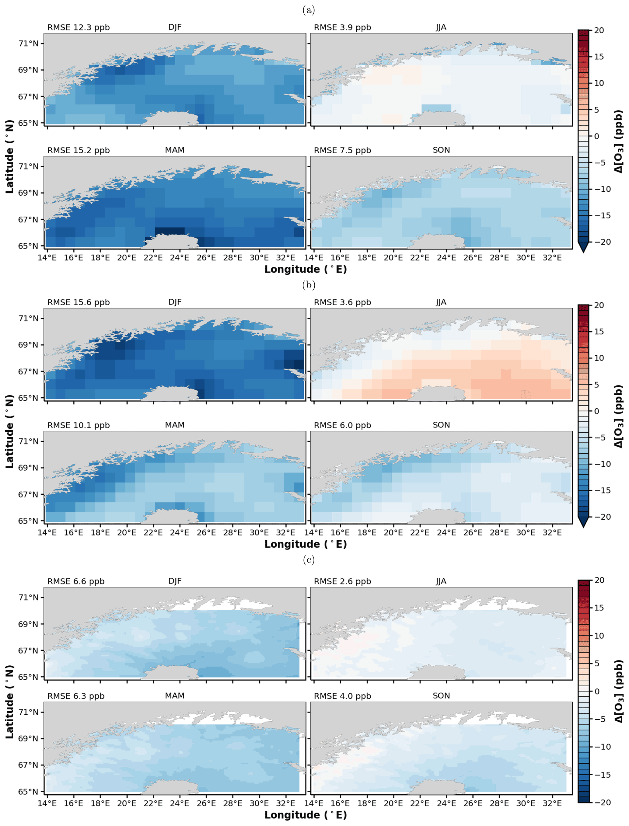
Figure 4Deviation of reanalysis products from generalized ozone climatology for northern Fennoscandia: (a) MACC, (b) CAMS, and (c) CAMSRAQ. Negative (positive) values indicate that the reanalysis product underestimates (overestimates) the ground-level background [O3]. Shown are seasonal averages: December–January–February (DJF), June–July–August (JJA), March–April–May (MAM), and September–October–November (SON). The RMSE has been computed over land only and is displayed in the upper left corner of each panel.
The performance of CAMSRAQ ensemble and each of its contributing models is continuously validated with data from active European monitoring stations south of 60.53∘ N. This validation is graphically provided at https://www.regional.atmosphere.copernicus.eu/evaluation.php?interactive=cda (last access: May 2021). Following the Copernicus Atmosphere Monitoring Service (2020a) guidelines, the analysis comprises mean bias, modified mean bias, RMSE, fractional gross error, and temporal correlations of the O3 daily maximum. The ensemble median of the O3 daily maximum shows the largest RMSE in JJA (5.28 ppb) and the smallest in MAM (4.05 ppb), which is contrary to our results for the daily mean O3. The mean bias oscillates between 0.97 ppb (DJF) and −1.77 ppb (JJA), which is also opposite to our evaluation in northern Fennoscandia with a small bias in JJA and a larger negative deviation from observations in DJF and MAM. This indicates that underlying uncertainties in CAMSRAQ manifest differently at higher latitudes. Enhancements lead to better model performances in mid latitudes and, hence, do not necessarily affect results in the Arctic and subarctic in the same way.
3.2 Implications on integrated flux quantities
As pointed out by Hayes et al. (2018), the highest sensitivity to differences in ozone concentrations occurs in coincidence with the highest productivity of plants in summer. The poor agreement between the global reanalysis products and observations in winter and fall may therefore have limited consequences on integrated flux quantities (e.g., PODy) used to assess the ozone risk on vegetation.
The computation of PODy is nontrivial and depends on state functions of the atmosphere, soil, and vegetation, as well as wind fields (Mills et al., 2017). In the following assessment, we, therefore, make some simplifications. We choose Svanvik as an example location for which we have meteorological conditions readily available and compute a cumulative uptake of ozone (CUO) with a threshold of y=0:
with . The time dependent ozone flux through the stomata is usually defined as
We neglect the quasi laminar (rb) and leaf surface resistance (rc) terms in the following. This can be justified by only looking at the relative percentage differences in the following and not the absolute CUO values. Ozone concentrations are converted from ppb to mmol m−3 by using the ideal gas law () and multiplying by 10−6. For simplicity, we assume standard pressure () but insert observed 2018 temperatures at Svanvik. The stomatal conductance follows from (Jarvis, 1976; Emberson et al., 2000; Mills et al., 2017):
with normalized response functions to light (flight), temperature (fT), vapor pressure deficit (fVPD), and soil water potential (fSWP), and the minimum (fmin) and maximum conductance (gmax). We assume a sufficiently moist soil and hence the dependency on soil water potential to be negligible (fSWP=1).
Meteorological data (temperature, relative humidity, global irradiance) from Svanvik in 2018 are used to compute gsto. Although 2018 was characterized by an extended drought period over large parts of Europe, northern Fennoscandia was affected to a lesser degree than the rest of Europe (Gangstø Skaland et al., 2019). We calculate CUO for parameterizations of boreal deciduous and coniferous trees (Table III.11 in Mills et al., 2017). We use the bias-corrected observed ozone climatology for Svanvik as a reference to probe the climatologies based on MACC, CAMSRA, and CAMSRAQ (Fig. 3). For this purpose, MACC and CAMSRA climatologies have been upsampled to 1-hourly resolution by linearly interpolating between existing values.
Table 3Relative percentage difference in CUO0 for the different ozone reanalysis products compared to observed ozone. Boreal parameterizations of deciduous and coniferous trees are taken from Mills et al. (2017).
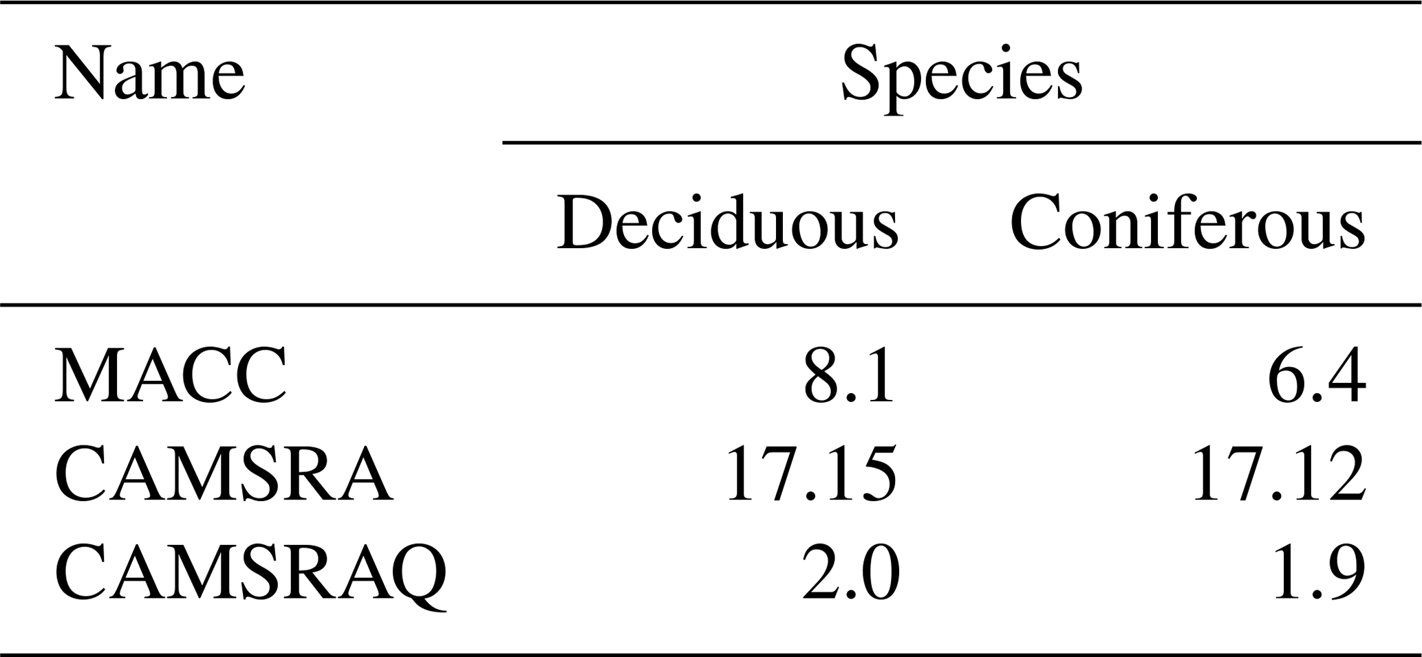
We find that all reanalysis products overestimate CUO compared to observations (Table 3). CAMSRAQ performs best displaying only a small deviation (2 %). While CAMSRA represented the seasonal cycle better than MACC (Sect. 3.1), its performance in terms of CUO is poor. This can be attributed to a pronounced bias towards higher ozone concentrations in CAMSRA during summer as emerges clearly from Fig. 4. The deficits of MACC in spring reduces CUO for coniferous trees and thus counters too high [O3] in summer.
3.3 Reconstruction of missing ozone data
Based on our assessment, only the CAMSRAQ product suffices for gap-filling. We shall now derive a reconstruction method based on a Reynolds decomposition for use in ozone impact studies on vegetation. We will compare the reconstructed data with an evaluation of CAMSRAQ at the nearest-neighbor grid point and compute the respective RSME values with respect to observed data before and after the gap.
The ozone data were taken at Svanvik in 2018. Due to problems in data acquisition, the data for 9–23 July 2018 are missing from the record. These coincide with large, active forest fires in central Sweden (Björklund et al., 2019), which presumably caused elevated concentrations of ozone precursors. Enhanced [O3] were observed throughout July and coincident peak concentrations above 40 ppb are found in the data series from Esrange and Pallas on 4, 12–16, 25, and 31 July (Fig. 6a). At Svanvik, the peak [O3] in early July was not observed but elevated [O3] occurred at the end of the month. During these forest-fire-induced pollution events, [O3] deviated from the respective climatology by up to 28 ppb (Fig. 6b). These special conditions demand a more elaborate gap-filling procedure than suggested by Mills et al. (2020). As described in Sect. 1, gap-filling is usually done by using mean values from the same period from previous years or by using mean values from the same time of day from previous days. Considering forest fires are rare events, those mean values will not be good candidates for gap-filling. In addition, data from a reference station selected based on a high correlation factor alone are not sufficient, because a correlation does not account for systematic offsets or the transport of pollutants.
A Reynolds decomposition is an analytical method often used in atmospheric and climate science to separate the expected value () of a variable u from its fluctuations (u′):
As expected value, we assume the averaged seasonal cycle from a subset of ozone monitoring data excluding the year of interest and refer to this as ozone climatology 〈[O3]〉. The fluctuations Δ[O3] (anomalies) for the year of interest are derived in accordance with Eq. (4):
To synchronize the time series temporally, we compute time-lagged correlations between Svanvik and the other stations in northern Fennoscandia during the overlapping periods in the 1990s (Fig. 5). To this end, we shift one series by Δt and find the respective Pearson correlation coefficient. The data show a correlation maximum with Esrange and Pallas at +3 and +1 h with Jergul/Karasjok. This means that these lag behind Svanvik. Of all stations, only Pallas displays a sufficiently high correlation with Svanvik (r2≥0.61) (Mills et al., 2020, Sect. 12.5). We, therefore, choose Pallas as the reference station for the following reconstruction procedure. We derive a projection of the generalized ozone climatology to Svanvik and account for the time lag by shifting the climatology by 3 h:
We apply Eq. (5) to derive 1-hourly anomalies compared to the generalized climatology for each active station in 2018
with i∈{Esrange, Pallas, Svanvik}.

Figure 5Temporal correlation of [O3] data between Svanvik and other ozone monitoring sites in northern Fennoscandia over time lag. The time-lag correlation has been computed by shifting one of the series by Δt. A negative lag means that Svanvik lags behind, while a positive lag mean the other station lags behind. The highest correlation with Pallas/Esrange is found at a time lag of 3 h for Jergul/Karasjok at 1 h.
Observational data for Svanvik, Esrange, and Pallas for July 2018 are depicted in Fig. 6a. For reference, we overlay the generalized climatology, the climatology for Svanvik in 1-hourly resolution, and indicate the time-lag-corrected generalized climatology.
We also correct the derived ozone anomalies at Pallas for the time-lag and use the projection (Eq. 6) to reconstruct anomalies for the missing values at Svanvik:
The result is depicted in Fig. 6b, where the 1-hourly ozone concentration anomalies are shown together with the reconstructed anomalies for Svanvik. We do not account for the transport of pollutants or advection of ozone in our reconstruction procedure which results in a prominent lag between the reconstruction and the observations on 25 and 26 July. In the context of risk assessment of ozone damage on vegetation, this has no large impact, as the applied flux-based metric PODy is usually integrated over a whole season (e.g., Mills et al., 2011).
Finally, we add these anomalies to the Svanvik climatology, account for the estimated bias due to the change in ground-level background ozone (δ[O3]=1.2 ppb), and derive the reconstructed time series:
In Fig. 6c, our reconstruction is shown together with the observed data before and after the gap and CAMSRAQ evaluated at the nearest-neighbor grid point. Both perform qualitatively well. To quantify the performance of our reconstruction and the CAMSRAQ, we compute RMSE values for the days in July for which observational data are available. We find a RSME=8.20 ppb for our reconstruction and RSME=7.52 ppb for the CAMSRAQ. This indicates that our reconstruction has an accuracy of about 76 % and its performance is comparable with CAMSRAQ (80 %) despite not accounting for atmospheric transport and chemical transformation explicitly. For comparison, the computed accuracy of data taken at Pallas in 2018 without further processing is decent (69 %), while data taken at Svanvik in July 2019 agree fairly well (72 %).
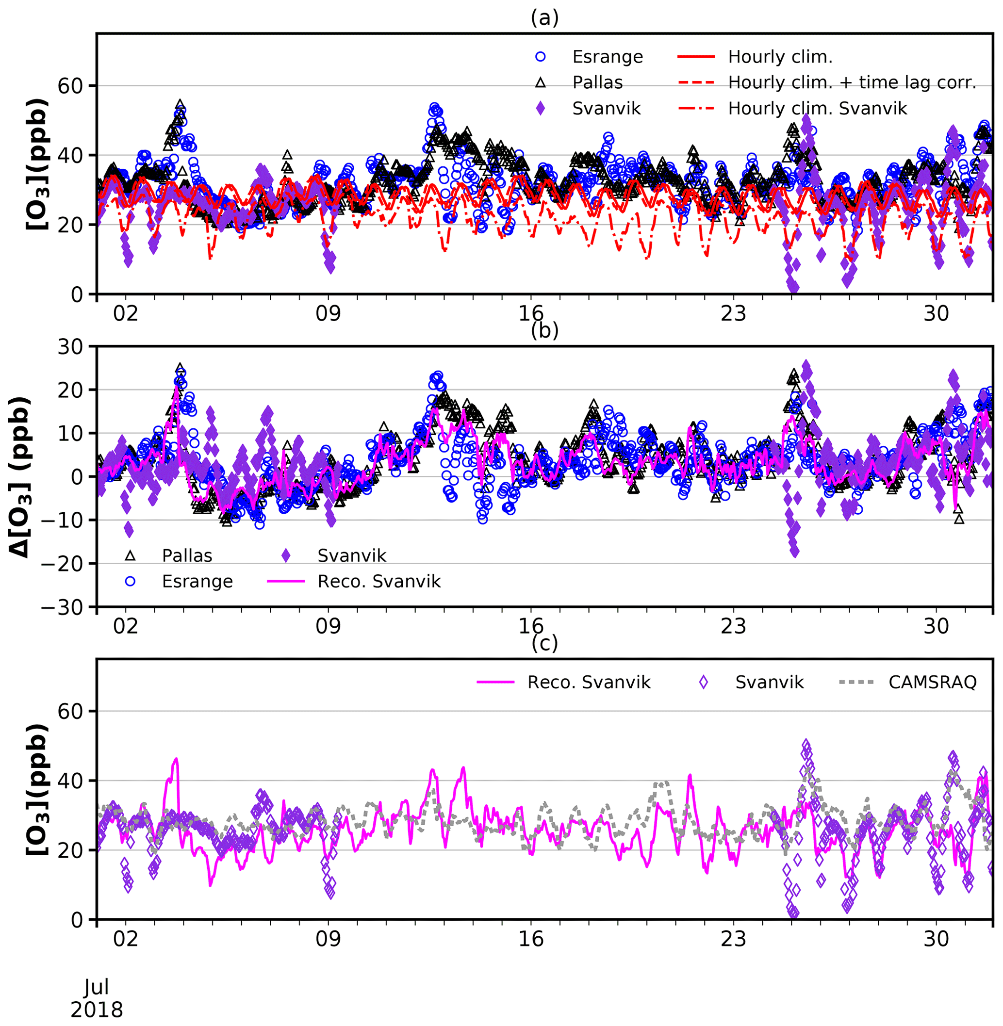
Figure 6Reconstruction procedure for missing [O3] data (9–23 July 2018). Observed 1-hourly [O3] values are shown together with 1-hourly climatologies derived for northern Fennoscandia (combined data from Esrange, Jergul/Karasjok, Pallas) and Svanvik. (a) Time series supplemented with 1-hourly climatologies. The time-lag correction of the northern Fennoscandia climatology is also indicated; (b) observed and reconstructed anomalies; (c) reconstructed [O3] for Svanvik in comparison with CAMSRAQ evaluated at the nearest-neighbor grid point.
We derived a representative ozone climatology for northern Fennoscandia based on long-term ground-level ozone monitoring in Finland, Norway, and Sweden. Based on this generalized ozone climatology, we assessed the quality of available global (MACC and CAMSRA) and regional (CAMSRAQ) reanalysis products for northern Fennoscandia focusing on the seasonality of ozone. We confirm previously published results concerning the quality of global reanalysis products (Huijnen et al., 2020; Barten et al., 2021) and find that the observed ozone patterns in northern Fennoscandia are not reproduced well. Better performance was displayed by the regional model reanalysis CAMSRAQ ensemble which reproduces the observed ozone seasonality well, although with a remaining annual average deviation of up to −7 ppb. All products showed deficits, in particular during winter and spring. Spatial patterns of deviation from the generalized climatology indicate a substantial underestimation of ozone abundance in the global reanalysis products on the west coast of northern Fennoscandia. This could be due to their spatial resolution, e.g., a high oceanic fraction in the coastal grid cells or representation of elevation. We confirm that a higher spatiotemporal resolution, assimilation of vertical ozone profiles, and if applicable assimilation of in situ observations at ground-level lead to better constrained reanalysis products, especially at high latitudes during times when the coverage by passive sounders aboard satellites is low.
There is a multitude of probable reasons for the differences found between the reanalysis products and observations. The enhancements which led from the MACC reanalysis to CAMSRA have been reported and discussed by Inness et al. (2019) on global scales. Amongst others, assimilation of ozone profiles from satellite retrieval (compared to column densities) and an upgraded ozone chemistry have led to an enhanced performance of CAMSRA, but a considerable bias remains (Huijnen et al., 2020). In particular, Barten et al. (2021) reported a pronounced underestimation for CAMSRA in the high Arctic (e.g., Summit, Greenland) and attribute this to an insufficient representation of a mechanistic dry deposition scheme to the ocean. The large deviation which we found in all seasons but summer points to either a deficit in modeled removal processes or too weak model constraints by data from passive sounders aboard satellites in polar winter. In particular, too high dry deposition velocities over snow- and ice-covered surfaces would not allow for a sufficient buildup of ozone and precursors in winter, leading to too low modeled ozone concentrations (Falk and Sinnhuber, 2018; Falk and Søvde Haslerud, 2019). Due to the higher spatial resolution of the regional air quality models, CAMSRAQ is capable of capturing small-scale depletion and peak episodes of ozone. The higher spatial and temporal resolution improves daily and seasonal cycles of modeled ozone which is especially important for use in risk assessment for vegetation damage and human health. Improvements in atmospheric transport as part of the OpenIFS updates may also play a role but cannot be assessed from our analysis. The higher spatial and temporal resolutions of CAMSRAQ aside, we can assume the assimilated ground-level ozone data were another driver for the different performances as passive sounders aboard satellites typically resolve [O3] at the surface rather poorly and hence do not constrain the global models well enough (Andersson et al., 2017).
To account for missing data from the 2018 record at Svanvik located in northern Norway, we proposed a routine for reconstruction of 1-hourly ozone data, adhering to the UNECE-LRTAP conventions (Mills et al., 2020). We performed a Reynolds decomposition into anomalies and climatology, identified a reference station with the highest Pearson correlation coefficient, synchronized the time series using a time-lag correlation, and corrected for a bias induced by the increase in ground-level background ozone concentrations since the end of the regular measurements at Svanvik in the mid-1990s. As we do not take atmospheric transport of pollutants into account, the reconstructed data display inaccuracies in the timing of peak episodes. This deficit, however, has no large impact in the context of risk assessment of ozone damage on vegetation, because the applied flux-based metrics typically integrate the ozone uptake over a whole season. Our devised reconstruction method's performance (76 % accuracy) is compatible with evaluating CAMSRAQ at the nearest-neighbor grid point (80 %) and better than standard methods (69 %–72 %). However, two criteria have to be met before our reconstruction can be performed: (1) availability of overlapping long-term series and (2) availability of overlapping data from a reasonably close-by site with a high Pearson correlation coefficient during the occurrence of the gap.
We have shown that the representation of ground-level ozone concentration in the global state-of-the-art reanalysis product CAMSRA is poor in winter but good in summer. In all seasons but summer, negative deviations occur over northern Fennoscandia. In summer, CAMSRA displays a pronounced bias towards higher-than-observed ozone concentrations (6 ppb) in regions east of the Scandinavian Mountains. The regional reanalysis product CAMSRAQ displays slightly too low ozone concentrations throughout all seasons, though, not significant in summer. To assess the impact of ozone on vegetation risks, we computed a relative cumulative uptake of ozone. Positive deviations in [O3] in summer compared to the generalized climatology for northern Fennoscandia cause a relative percentage deviation of CAMSRA of 17 %. For the MACC reanalysis, we find 7 %. The lower deviation does not indicate better performance but is due to the pronounced underestimation of [O3] in spring, countering too high ozone abundances in summer. This is also reflected by diverging results for coniferous and deciduous trees. CAMSRAQ deviates by only 2 % confirming its suitability for vegetation risk assessments. Our results are in line with Hayes et al. (2018), who showed that a climate-change-induced increase in summer ground-level ozone concentration can affect the stomatal uptake of ozone in southwestern Sweden on the order of 3 %–16 %. Environmental conditions in spring and fall limit the effects for most species, except for coniferous species which are photosynthetically active at low temperatures and could be moderately affected.
Our devised gap-filling method is to be preferred over data from close-by stations or data from the same period but different years. Overall, CAMSRAQ showed the best performance. We can therefore recommend using CAMSRAQ for gap-filling of ozone monitoring data. It is also a valid choice for ozone risk assessment on vegetation in northern Fennoscandia. Global reanalysis products are not recommended for this purpose.
Python 2.7 code is available under Creative Commons license on the GitHub repository ozone_anomalies of the corresponding author (https://github.com/ziu1986/python_scripts/tree/master/ozone_metrics/ozone_anomalies, Falk, 2021). Please get in touch for further information.
All observational data are available form NILU's EBAS database. MACC and CAMS reanalysis data are available through ECMWF's data services. CAMSRAQ is available from the regional atmosphere data service of Copernicus.
SF acquired and processed all data, conducted the analysis, and composed the figures and manuscript. AVV and FS contributed to proofreading. All authors contributed to discussion.
The contact author has declared that neither they nor their co-authors have any competing interests.
Publisher’s note: Copernicus Publications remains neutral with regard to jurisdictional claims in published maps and institutional affiliations.
We would also like to thank the LATICE research group and the EMERALD project (294948) for supporting this work.
This research has been supported by the Norges Forskningsråd (grant no. 268073).
This paper was edited by Jens-Uwe Grooß and reviewed by two anonymous referees.
Ainsworth, E. A.: Understanding and improving global crop response to ozone pollution, Plant J., 90, 886–897, https://doi.org/10.1111/tpj.13298, 2017. a
Andersson, C., Alpfjord, H., Robertson, L., Karlsson, P. E., and Engardt, M.: Reanalysis of and attribution to near-surface ozone concentrations in Sweden during 1990–2013, Atmos. Chem. Phys., 17, 13869–13890, https://doi.org/10.5194/acp-17-13869-2017, 2017. a, b
Barten, J. G. M., Ganzeveld, L. N., Steeneveld, G.-J., and Krol, M. C.: Role of oceanic ozone deposition in explaining temporal variability in surface ozone at High Arctic sites, Atmos. Chem. Phys., 21, 10229–10248, https://doi.org/10.5194/acp-21-10229-2021, 2021. a, b, c, d
Björklund, J.-Å., Ekelund, K., Henningsson, A., Perers, K., Peters, J., Siverstig, A., Uddholm, L.-G., and Wisén, J.: Betänkande av 2018 års skogsbrandsutredning, SOU2019 7, Statens Offentliga Utredningar (SOU), available at: https://www.regeringen.se/rattsliga-dokument/statens-offentliga-utredningar/2019/02/sou-20197/ (last access: April 2020), 2019. a
Chuwah, C., van Noije, T., van Vuuren, D. P., Stehfest, E., and Hazeleger, W.: Global impacts of surface ozone changes on crop yields and land use, Atmos. Environ., 106, 11–23, https://doi.org/10.1016/j.atmosenv.2015.01.062, 2015. a
Clifton, O., Fiore, A., Massman, W., Baublitz, C., Coyle, M., Emberson, L., Fares, S., Farmer, D., Gentine, P., Gerosa, G., Guenther, A., Helmig, D., Lombardozzi, D., Munger, J., Patton, E., Pusede, S., Schwede, D., Silva, S., Sörgel, M., and Tai, A.: Dry Deposition of Ozone Over Land: Processes, Measurement, and Modeling, Rev. Geophys., e2019RG000670, https://doi.org/10.1029/2019RG000670, 2020. a
Cooper, O., Parrish, D., Ziemke, J., Balashov, N., Cupeiro, M., Galbally, I., Gilge, S., Horowitz, L., Jensen, N., Lamarque, J.-F., Naik, V., Oltmans, S., Schwab, J., Shindell, D., Thompson, A., Thouret, V., Wang, Y., and Zbinden, R.: Global distribution and trends of tropospheric ozone: An observation-based review, Elementa-Sci Anthrop., 2, 000029, https://doi.org/10.12952/journal.elementa.000029, 2014. a
Copernicus Atmosphere Monitoring Service: Verification plots: documentation, available at: http://macc-raq-op.meteo.fr/doc/USER_GUIDE_VERIFICATION_STATISTICS.pdf (last access: May 2021), 2020a. a
Copernicus Atmospheric Monitoring Service: CAMS Regional Air Quality reanalysis, available at: http://macc-raq-op.meteo.fr/index.php?category=data_access&subensemble=reanalysis_products, last access: July 2020b. a
Emberson, L.: Effects of ozone on agriculture, forests and grasslands, Philosophical transactions. Series A, Mathematical, physical, and engineering sciences, 378, 20190327, https://doi.org/10.1098/rsta.2019.0327, 2020. a
Emberson, L. D., for Monitoring, C. P., of the Long Range Transmission of Air Pollutants in Europe, E., meteorologiske institutt, N., and Meteorological Synthesizing Centre-West (Oslo, N.: Towards a Model of Ozone Deposition and Stomatal Uptake Over Europe, EMEP/MSC-W Note, Norwegian Meteorological Institute, available at: https://books.google.no/books?id=hj_ntgAACAAJ (last access: May 2019), 2000. a
Falk, S.: numerical recipe, python_scripts/ozone_metrics/ozone_anomalies/, GitHub [code], available at: https://github.com/ziu1986/python_scripts/tree/master/ozone_metrics/ozone_anomalies, last access: 14 October 2021. a
Falk, S. and Sinnhuber, B.-M.: Polar boundary layer bromine explosion and ozone depletion events in the chemistry–climate model EMAC v2.52: implementation and evaluation of AirSnow algorithm, Geosci. Model Dev., 11, 1115–1131, https://doi.org/10.5194/gmd-11-1115-2018, 2018. a
Falk, S. and Søvde Haslerud, A.: Update and evaluation of the ozone dry deposition in Oslo CTM3 v1.0, Geosci. Model Dev., 12, 4705–4728, https://doi.org/10.5194/gmd-12-4705-2019, 2019. a
Fleming, Z. L., Doherty, R. M., von Schneidemesser, E., Malley, C. S., Cooper, O. R., Pinto, J. P., Colette, A., Xu, X., Simpson, D., Schultz, M. G., Lefohn, A. S., Hamad, S., Moolla, R., Solberg, S., and Feng, Z.: Tropospheric Ozone Assessment Report: Present-day ozone distribution and trends relevant to human health, Elementa-Sci Anthrop., 6, 12, https://doi.org/10.1525/elementa.273, 2018. a
Franz, M. and Zaehle, S.: Competing effects of nitrogen deposition and ozone exposure on northern hemispheric terrestrial carbon uptake and storage, 1850–2099, Biogeosciences, 18, 3219–3241, https://doi.org/10.5194/bg-18-3219-2021, 2021. a
Gangstø Skaland, R., Colleuille, H., Håvelsrud Andersen, A. S., Mamen, J., Grinde, L., Tajet, H. T. T., Lundstad, E., Sidselrud, L. F., Tunheim, K., Hanssen-Bauer, I., Benestad, R., Heiberg, H., and Hygen, H. O.: Tørkesommeren 2018, METinfo 14, Norwegian Meteorological Institute, available at: https://www.met.no/publikasjoner/met-info/met-info-2019 (last access: March 2020), 2019. a
Gaudel, A., Cooper, O. R., Ancellet, G., Barret, B., Boynard, A., Burrows, J. P., Clerbaux, C., Coheur, P. F., Cuesta, J., Cuevas, E., Doniki, S., Dufour, G., Ebojie, F., Foret, G., Garcia, O., Granados-Munoz, M. J., Hannigan, J. W., Hase, F., Hassler, B., Huang, G., Hurtmans, D., Jaffe, D., Jones, N., Kalabokas, P., Kerridge, B., Kulawik, S., Latter, B., Leblanc, T., Le Flochmoen, E., Lin, W., Liu, J., Liu, X., Mahieu, E., McClure-Begley, A., Neu, J. L., Osman, M., Palm, M., Petetin, H., Petropavlovskikh, I., Querel, R., Rahpoe, N., Rozanov, A., Schultz, M. G., Schwab, J., Siddans, R., Smale, D., Steinbacher, M., Tanimoto, H., Tarasick, D. W., Thouret, V., Thompson, A. M., Trickl, T., Weatherhead, E., Wespes, C., Worden, H. M., Vigouroux, C., Xu, X., Zeng, G., and Ziemke, J.: Tropospheric Ozone Assessment Report: Present-day distribution and trends of tropospheric ozone relevant to climate and global atmospheric chemistry model evaluation, Elementa-Sci Anthrop., 6, 39, https://doi.org/10.1525/elementa.291, 2018. a
Hatakka, J., Aalto, T., Aaltonen, V., Aurela, M., Hakola, H., Komppula, M., Laurila, T., Lihavainen, H., Paatero, J., Salminen, K., and Viisanen, Y.: Overview of the atmospheric research activities and results at Pallas GAW station, Boreal Environ. Res., 8, 365–383, 2003. a
Hayes, F., Mills, G., Alonso, R., González, I., Coyle, M., Grünhage, L., Gerosa, G., Karlsson, P., and Marzuoli, R.: A Site-Specific Analysis of the Implications of a Changing Ozone Profile and Climate for Stomatal Ozone Fluxes in Europe, Water Air Soil Poll., 230, 1–15, https://doi.org/10.1007/s11270-018-4057-x, 2018. a, b
Høgda, K., Tømmervik, H., and Karlsen, S.: Trends in the Start of the Growing Season in Fennoscandia 1982-2011, Remote Sens., 5, 4304–4318, https://doi.org/10.3390/rs5094304, 2013. a
Hoshika, Y., Katata, G., Deushi, M., Watanabe, M., Koike, T., and Paoletti, E.: Ozone-induced stomatal sluggishness changes carbon and water balance of temperate deciduous forests, Sci. Rep.-UK, 5, 09871, https://doi.org/10.1038/srep09871, 2015. a
Huijnen, V., Miyazaki, K., Flemming, J., Inness, A., Sekiya, T., and Schultz, M. G.: An intercomparison of tropospheric ozone reanalysis products from CAMS, CAMS interim, TCR-1, and TCR-2, Geosci. Model Dev., 13, 1513–1544, https://doi.org/10.5194/gmd-13-1513-2020, 2020. a, b, c, d, e
Inness, A., Baier, F., Benedetti, A., Bouarar, I., Chabrillat, S., Clark, H., Clerbaux, C., Coheur, P., Engelen, R. J., Errera, Q., Flemming, J., George, M., Granier, C., Hadji-Lazaro, J., Huijnen, V., Hurtmans, D., Jones, L., Kaiser, J. W., Kapsomenakis, J., Lefever, K., Leitão, J., Razinger, M., Richter, A., Schultz, M. G., Simmons, A. J., Suttie, M., Stein, O., Thépaut, J.-N., Thouret, V., Vrekoussis, M., Zerefos, C., and the MACC team: The MACC reanalysis: an 8 yr data set of atmospheric composition, Atmos. Chem. Phys., 13, 4073–4109, https://doi.org/10.5194/acp-13-4073-2013, 2013. a
Inness, A., Ades, M., Agustí-Panareda, A., Barré, J., Benedictow, A., Blechschmidt, A.-M., Dominguez, J. J., Engelen, R., Eskes, H., Flemming, J., Huijnen, V., Jones, L., Kipling, Z., Massart, S., Parrington, M., Peuch, V.-H., Razinger, M., Remy, S., Schulz, M., and Suttie, M.: The CAMS reanalysis of atmospheric composition, Atmos. Chem. Phys., 19, 3515–3556, https://doi.org/10.5194/acp-19-3515-2019, 2019. a, b
Hartmann, D. L., Klein Tank, A. M. G., Rusticucci, M., Alexander, L. V., Brönnimann, S., Charabi, Y., Dentener, F. J., Dlugokencky, E. J., Easterling, D. R., Kaplan, A., Soden, B. J., Thorne, P. W., Wild, M., and Zhai, P. M.: Observations: Atmosphere and Surface, in: Climate Change 2013: The Physical Science Basis. Contribution of Working Group I to the Fifth Assessment Report of the Intergovernmental Panel on Climate Change, chap. 2, 159–254, edited by: Stocker, T. F., Qin, D., Plattner, G.-K., Tignor, M., Allen, S. K., Boschung, J., Nauels, A., Xia, Y., Bex, V., and Midgley, P. M., Cambridge University Press, Cambridge, United Kingdom and New York, NY, USA, https://doi.org/10.1017/CBO9781107415324.008, 2013. a
Jarvis, P. G.: The interpretation of the variations in leaf water potential and stomatal conductance found in canopies in the field, Philos. T. Roy. Soc. B., 273, 593–610, https://doi.org/10.1098/rstb.1976.0035, 1976. a
Kangaskärvi, J., Jaspers, P., and Kollist, H.: Signalling and cell death in ozone-exposed plants, Plant Cell Environ., 28, 1021–1036, https://doi.org/10.1111/j.1365-3040.2005.01325.x, 2005. a
Karlsen, S., Solheim, I., Beck, P., Høgda, K., Wielgolaski, F., and Tømmervik, H.: Variability of the start of the growing season in Fennoscandia, 1982–2002, Int. J. Biometeorol., 51, 513–24, https://doi.org/10.1007/s00484-007-0091-x, 2007. a
Karlsson, P., Ferm, M., Tømmervik, H., Hole, L., Karlsson, G., Ruoho-Airola, T., Aas, W., Hellsten, S., Akselsson, C., Mikkelsen, T., and Nihlgård, B.: Biomass burning in eastern Europe during spring 2006 caused high deposition of ammonium in northern Fennoscandia, Environ. Pollut., 176, 71–79, https://doi.org/10.1016/j.envpol.2012.12.006, 2013. a
Karlsson, P. E., Pleijel, H., Andersson, C., Bergström, R., Engardt, M., Eriksen, A., Falk, S., Klingberg, J., Langner, J., Manninen, S., Stordal, F., Tømmervik, H., and Vollsnes, A.: The vulnerability of northern European vegetation to ozone damage in a changing climate - An assessment based on current knowledge, Tech. Rep. C586, IVL Svenska Miljöinstitutet, available at: https://www.ivl.se/publikationer/publikation.html?id=6220 (last access: May 2021), 2021. a
Kobayashi, S., Ota, Y., Harada, Y., Ebita, A., Moriya, M., Onoda, H., Onogi, K., Kamahori, H., Kobayashi, C., Endo, H., Miyaoka, K., and Takahashi, K.: The JRA-55 Reanalysis: General Specifications and Basic Characteristics, J. Meteor. Soc. Jpn., 93, 5–48, https://doi.org/10.2151/jmsj.2015-001, 2015. a
Linderholm, H.: Growing Season Changes in the Last Century, Agr. Forest Meteorol., 137, 1–14, https://doi.org/10.1016/j.agrformet.2006.03.006, 2006. a
Lindskog, A., Karlsson, P., Grennfelt, P., Solberg, S., and Forster, C.: An exceptional ozone episode in northern Fennoscandia, Atmos. Environ., 41, 950–958, https://doi.org/10.1016/j.atmosenv.2006.09.027, 2007. a
Lombardozzi, D., Bonan, G. B., Smith, N. G., Dukes, J. S., and Fisher, R. A.: Temperature acclimation of photosynthesis and respiration: A key uncertainty in the carbon cycle-climate feedback, Geophys. Res. Lett., 42, 8624–8631, https://doi.org/10.1002/2015GL065934, 2015a. a
Lombardozzi, D., Levis, S., Bonan, G., Hess, P., and Sparks, J.: The Influence of Chronic Ozone Exposure on Global Carbon and Water Cycles, J. Climate, 28, 292–305, https://doi.org/10.1175/JCLI-D-14-00223.1, 2015b. a
Mills, G., Hayes, F., Simpson, D., Emberson, L., Norris, D., Harmens, H., and Büker, P.: Evidence of widespread effects of ozone on crops and (semi‐)natural vegetation in Europe (1990–2006) in relation to AOT40- and flux-based risk maps, Glob. Change Biol., 17, 592–613, https://doi.org/10.1111/j.1365-2486.2010.02217.x, 2011. a, b, c
Mills, G., Sharps, K., Simpson, D., Pleijel, H., Broberg, M., Uddling, J., Jaramillo, F., Davies, W. J., Dentener, F., Van den Berg, M., Agrawal, M., Agrawal, S. B., Ainsworth, E. A., Büker, P., Emberson, L., Feng, Z., Harmens, H., Hayes, F., Kobayashi, K., Paoletti, E., and Van Dingenen, R.: Ozone pollution will compromise efforts to increase global wheat production, Glob. Change Biol., 24, 3560–3574, https://doi.org/10.1111/gcb.14157, 2018. a
Mills, G., Harmens, H., Hayes, F., Pleijel, H., Büker, P., González-Fernandéz, I., Alonso, R., Bender, J., Bergmann, E. Bermejo, V., Braun, S., Danielsson, H., Gerosa, G., Grünhage, L., Karlsson, P. E., Marzuoli, R., Schaub, M., and Simpson, D.: ICP Mapping Manual - Chapter III: Mapping Critical Levels for Vegetation, International Cooperative Programme on Effects of Air Pollution on Natural Vegetation and Crops, available at: https://www.umweltbundesamt.de/en/Coordination_Centre_for_Effects (last access: February 2019), minor edits OCT 2017, 2017. a, b, c, d
Mills, G., Pleijel, H., Malley, C. S., Sinha, B., Cooper, O. R., Schultz, M. G., Neufeld, H. S., Simpson, D., Sharps, K., Feng, Z., Gerosa, G., Harmens, H., Kobayashi, K., Saxena, P., Paoletti, E., Sinha, V., and Xu, X.: Tropospheric Ozone Assessment Report: Present-day tropospheric ozone distribution and trends relevant to vegetation, Elementa-Sci Anthrop., 6, 47, https://doi.org/10.1525/elementa.302, 2018. a
Mills, G., Harmens, H., Hayes, F., Pleijel, H., Büker, P., González-Fernandéz, I., Alonso, R., Hayes, F., and Sharps, K.: Scientific background document B – developing areas of research of relevance to chapter III (mapping critical levels for vegetation) of the modelling and mapping manual of the lrtap convention, International Cooperative Programme on Effects of Air Pollution on Natural Vegetation and Crops, available at: https://icpvegetation.ceh.ac.uk/get-involved/manuals/mapping-manual (last access: May 2021), 2020. a, b, c, d, e
Miyazaki, K., Bowman, K., Sekiya, T., Eskes, H., Boersma, F., Worden, H., Livesey, N., Payne, V. H., Sudo, K., Kanaya, Y., Takigawa, M., and Ogochi, K.: Updated tropospheric chemistry reanalysis and emission estimates, TCR-2, for 2005–2018, Earth Syst. Sci. Data, 12, 2223–2259, https://doi.org/10.5194/essd-12-2223-2020, 2020. a
Monks, P. S.: A review of the observations and origins of the spring ozone maximum, Atmos. Environ., 34, 3545–3561, https://doi.org/10.1016/S1352-2310(00)00129-1, 2000. a
Monks, P. S., Archibald, A. T., Colette, A., Cooper, O., Coyle, M., Derwent, R., Fowler, D., Granier, C., Law, K. S., Mills, G. E., Stevenson, D. S., Tarasova, O., Thouret, V., von Schneidemesser, E., Sommariva, R., Wild, O., and Williams, M. L.: Tropospheric ozone and its precursors from the urban to the global scale from air quality to short-lived climate forcer, Atmos. Chem. Phys., 15, 8889–8973, https://doi.org/10.5194/acp-15-8889-2015, 2015. a, b
Myhre, G., Shindell, D., Bréon, F.-M., Collins, W., Fuglestvedt, J., Huang, J., Koch, D., Lamarque, J.-F., Lee, D., Mendoza, B., Nakajima, T., Robock, A., Stephens, G., Takemura, T., and Zhang, H.: Anthropogenic and Natural Radiative Forcing, book section 8, Cambridge University Press, Cambridge, United Kingdom and New York, NY, USA, 659–740, https://doi.org/10.1017/CBO9781107415324.018, 2013. a
NILU: ebas.nilu.no website, available at: http://ebas.nilu.no/, last access: July 2020. a
Pellegrini, E., Francini, A., Lorenzini, G., and Nali, C.: PSII photochemistry and carboxylation efficiency in Liriodendron tulipifera under ozone exposure, Environ. Exp. Bot., 70, 217–226, 2011. a
Solberg, S.: Monitoring of boundary layer ozone in Norway from 1977 to 2002, Ozone Report 2003 85, Norwegian Institute for Air Research (NILU), 51 pp., 2003. a, b
Stevenson, D. S., Dentener, F. J., Schultz, M. G., Ellingsen, K., van Noije, T. P. C., Wild, O., Zeng, G., Amann, M., Atherton, C. S., Bell, N., Bergmann, D. J., Bey, I., Butler, T., Cofala, J., Collins, W. J., Derwent, R. G., Doherty, R. M., Drevet, J., Eskes, H. J., Fiore, A. M., Gauss, M., Hauglustaine, D. A., Horowitz, L. W., Isaksen, I. S. A., Krol, M. C., Lamarque, J.-F., Lawrence, M. G., Montanaro, V., Müller, J.-F., Pitari, G., Prather, M. J., Pyle, J. A., Rast, S., Rodriguez, J. M., Sanderson, M. G., Savage, N. H., Shindell, D. T., Strahan, S. E., Sudo, K., and Szopa, S.: Multimodel ensemble simulations of present-day and near-future tropospheric ozone, J. Geophys. Res.-Atmos., 111, 1–23, https://doi.org/10.1029/2005JD006338, 2005. a
Tai, A. P. K., Martin, M. V., and Heald, C. L.: Threat to future global food security from climate change and ozone air pollution, Nat. Clim. Change, 4, 817–821, https://doi.org/10.1038/NCLIMATE2317, 2014. a
Tang, H., Takigawa, M., Liu, G., Zhu, J., and Kobayashi, K.: A projection of ozone-induced wheat production loss in China and India for the years 2000 and 2020 with exposure-based and flux-based approaches, Glob. Change Biol., 19, 2739–2752, https://doi.org/10.1111/gcb.12252, 2013. a
Škerlak, B., Sprenger, M., Pfahl, S., Tyrlis, E., and Wernli, H.: Tropopause folds in ERA-Interim: Global climatology and relation to extreme weather events, J. Geophys. Res.-Atmos., 120, 4860–4877, https://doi.org/10.1002/2014JD022787, 2015. a
Watanabe, M., Hoshika, Y., and Koike, T.: Photosynthetic responses of Monarch birch seedlings to differing timings of free air ozone fumigation, J. Plant Res., 127, 339–345, https://doi.org/10.1007/s10265-013-0622-y, 2014. a
Wespes, C., Hurtmans, D., Clerbaux, C., Boynard, A., and Coheur, P.-F.: Decrease in tropospheric O3 levels in the Northern Hemisphere observed by IASI, Atmos. Chem. Phys., 18, 6867–6885, https://doi.org/10.5194/acp-18-6867-2018, 2018. a
WHO – World Health Organization: Health risks of ozone from long-range transboundary air pollution, 36 pp., 2008. a
Young, P. J., Archibald, A. T., Bowman, K. W., Lamarque, J.-F., Naik, V., Stevenson, D. S., Tilmes, S., Voulgarakis, A., Wild, O., Bergmann, D., Cameron-Smith, P., Cionni, I., Collins, W. J., Dalsøren, S. B., Doherty, R. M., Eyring, V., Faluvegi, G., Horowitz, L. W., Josse, B., Lee, Y. H., MacKenzie, I. A., Nagashima, T., Plummer, D. A., Righi, M., Rumbold, S. T., Skeie, R. B., Shindell, D. T., Strode, S. A., Sudo, K., Szopa, S., and Zeng, G.: Pre-industrial to end 21st century projections of tropospheric ozone from the Atmospheric Chemistry and Climate Model Intercomparison Project (ACCMIP), Atmos. Chem. Phys., 13, 2063–2090, https://doi.org/10.5194/acp-13-2063-2013, 2013. a
Zhu, J., Tai, A. P. K., and Yim, S. H. L.: Effects of ozone-vegetation interactions on meteorology and air quality in China using a two-way coupled land-atmosphere model, Atmos. Chem. Phys. Discuss. [preprint], https://doi.org/10.5194/acp-2021-165, in review, 2021. a