the Creative Commons Attribution 4.0 License.
the Creative Commons Attribution 4.0 License.
 | 10 Aug 2021
The effect of forced change and unforced variability in heat waves, temperature extremes, and associated population risk in a CO2-warmed world
Jeffrey C. Mast
Andrew E. Dessler
This study investigates the impact of global warming on heat and humidity extremes by analyzing 6 h output from 28 members of the Max Planck Institute Grand Ensemble driven by forcing from a 1 % yr−1 CO2 increase. We find that unforced variability drives large changes in regional exposure to extremes in different ensemble members, and these variations are mostly associated with El Niño–Southern Oscillation (ENSO) variability. However, while the unforced variability in the climate can alter the occurrence of extremes regionally, variability within the ensemble decreases significantly as one looks at larger regions or at a global population perspective. This means that, for metrics of extreme heat and humidity analyzed here, forced variability in the climate is more important than the unforced variability at global scales. Lastly, we found that most heat wave metrics will increase significantly between 1.5 and 2.0 ∘C, and that low gross domestic product (GDP) regions show significantly higher risks of facing extreme heat events compared to high GDP regions. Considering the limited economic adaptability of the population to heat extremes, this reinforces the idea that the most severe impacts of climate change may fall mostly on those least capable of adapting.
- Article
(7702 KB) - Full-text XML
- BibTeX
- EndNote


-
The unforced variability in the climate system, primarily ENSO, plays a key role in the occurrence of extreme events in a warming world.
-
The uncertainty of unforced variability becomes smaller as one looks at larger regions or at a global perspective.
-
The increases in heat wave indices are significant between 1.5 and 2.0 ∘C of warming, and the risk of facing extreme heat events is higher in low GDP regions.
The long-term goal of the 2015 Paris Agreement is to keep the increase in global temperature well below 2 ∘C above preindustrial levels, while pursuing efforts and limiting the warming to 1.5 ∘C. Given that no one lives in the global average, however, understanding how these global average thresholds translate into regional occurrences of extreme heat and humidity is of great value (Harrington et al., 2018). Previous studies have reported that regional extreme heat events will not only be more frequent but also more extreme in a warmer world. This was discussed in various assessments and reports, such as National Climate Assessment (USA) and those by the IPCC (Intergovernmental Panel on Climate Change; Melillo et al., 2014; Wuebbles et al., 2017; Hoegh-Guldberg et al., 2018; Masson-Delmotte et al., 2018), and it is expected to have significant impacts on human society and health. More importantly, previous studies have analyzed the risk (Quinn et al., 2014; Sun et al., 2014; Lundgren et al., 2013), exposure (Dahl et al., 2019; Ruddell et al., 2009; Liu et al., 2017; Luber and McGeehin, 2008), vulnerability (Chow et al., 2012; Wilhelmi and Hayden, 2010), and susceptibility (Arbuthnott et al., 2016) of the population in the current and warmer climates.
Many criteria and indices have been used to assess extreme heat, such as the absolute increase in maximum temperature from the reference period (Wobus et al., 2018), the risk ratio of population's exposure to heat (Kharin et al., 2018), and the heat wave magnitude index (Russo et al., 2017). In this study, we utilize four locally defined heat wave indices from Fischer and Schär (2010) and Perkins et al. (2012) in terms of the duration, frequency, amplitude, and mean. We also focus on consecutive-day extremes, which are known to cause more harm than single-day events (Baldwin et al., 2019; Simolo et al., 2011; Tan et al., 2010). In addition, because the combined effect of temperature and humidity is known to affect human health by reducing the body's ability to cool itself through perspiration, wet bulb temperature is frequently analyzed (Kang and Eltahir, 2018). Wet bulb temperature is also closely associated with moist thermodynamics that drive the heat wave (Schwingshackl et al., 2021; Zhang et al., 2021), so we will analyze wet bulb temperature too.
Climate extremes are always a combination of long-term forced climate change acting in concert with unforced variability (Deser et al., 2012). Thus, characterizing and quantifying both long-term change due to external forcing and the unforced variability in the climate system is crucial for assessing the future risk of extreme events. There have been numerous studies that link dominant modes of unforced variability to extreme events. For example, previous studies have investigated temperature connections with the El Niño–Southern Oscillation (ENSO; Thirumalai et al., 2017; Meehl et al., 2007), the Pacific Decadal Oscillation (PDO; Birk et al., 2010), and the Atlantic Multidecadal Oscillation (AMO; Zhang et al., 2020; Mann et al., 2021). The effect of climate extremes on different populations depends on numerous factors, including the level of economic development, with impacts of heat extremes being more severe in less economically developed countries (Diffenbaugh and Burke, 2019; Harrington et al., 2016; King and Harrington, 2018; de Lima et al., 2021). For example, as temperatures go up, an increased energy demand to cool buildings will be required (Parkes et al., 2019; Sivak, 2009) in metropolitan areas. But this requires resources to both install air conditioning and operate it. The greater impacts of extreme heat in economically less developed regions in a warmer climate have been discussed in multiple studies (Marcotullio et al., 2021; Russo et al., 2019).
In this paper, a single-model initial-condition ensemble of 28 simulations of a global climate model (GCM) are used to quantify heat and humidity extremes in a warmer world. We use population data to look at the population risk for mortality events in the daytime (Mora et al., 2017) and nighttime (Chen and Lu, 2014). We also utilize per capita gross domestic product (GDP per capita) data to investigate how climate change impacts extreme heat events on different levels of economic status. To quantify the impact on energy demand, we also quantify the changes in cooling degree days and warming degree days.
2.1 MPI–GE ensembles
Simulation data in this study come from an ensemble of runs of the Max Plank Institute Earth System Model, collectively known as the MPI Grand Ensemble (MPI–GE) project (Maher et al., 2019). Each of the 28 ensemble members branches from different points of a 2000-year preindustrial control run and is integrated for 150 years, forced by a CO2 concentration increasing at 1 % yr−1 (hereafter, 1 % runs). Because the radiative forcing scales the log of the CO2 concentration, the 1 % runs feature radiative forcing that increases approximately linearly in time. We analyze 6 h output, with spatial resolution, which is the original resolution of the model output for land areas between 60∘ N and 60∘ S. Our analysis will focus on 2 m temperature (hereafter, t2m) and 2 m dew point temperature (d2m), from which 2 m relative humidity (RH) and wet bulb temperature (w2m) are calculated, using the methods of Davies-Jones (2008) with a predesigned module named HumanIndexMod (Buzan et al., 2015).
Unforced variability in the climate system generates uncertainties in the projection of the climate by impacting the dynamic component of the climate, especially for extreme events (Kay et al., 2015; Thompson et al., 2015). One way to analyze the impact of unforced variability in a climate system is to use an initial-condition ensemble. Each member of the initial-condition ensemble is generated by perturbating the initial conditions of single climate model. This perturbation will then propagate to generate different sequence of climate, such as ENSO, PDO, etc. (Deser et al., 2012; Kay et al., 2015). In this paper, we use the ensemble to allow us to estimate the impact of unforced variability in temperature extremes.
Since the model used only considers CO2 forcing without aerosols, and it represents a continuously warming climate, one might question if the model simulation accurately represents the real climate. To judge the fidelity of the simulations, we compare 15 years (2003–2017) of ERA-Interim reanalysis data (Dee et al., 2011) from the European Centre for Medium-Range forecast (ECMWF) with 15 years of the MPI–GE 1 % ensemble which have the same ensemble and global average temperatures (years 39–53); in the rest of the paper, we will refer to these as the reference periods. In both data sets, we then calculate 90th percentile and mean t2m and w2m for each grid point. This calculation was done for each member of the model ensemble. For each of the four values (90th percentile – t2m and w2m; mean – t2m and w2m), we determine if the values from the reanalysis fall into the spread of the 28 ensemble members of the 1 % runs. For each grid point, if the reanalysis value falls within the ensemble spread, we mask out the grid point; if not, we plot how far the reanalysis value is from the closest member of the 1 % ensemble (Fig. 1).
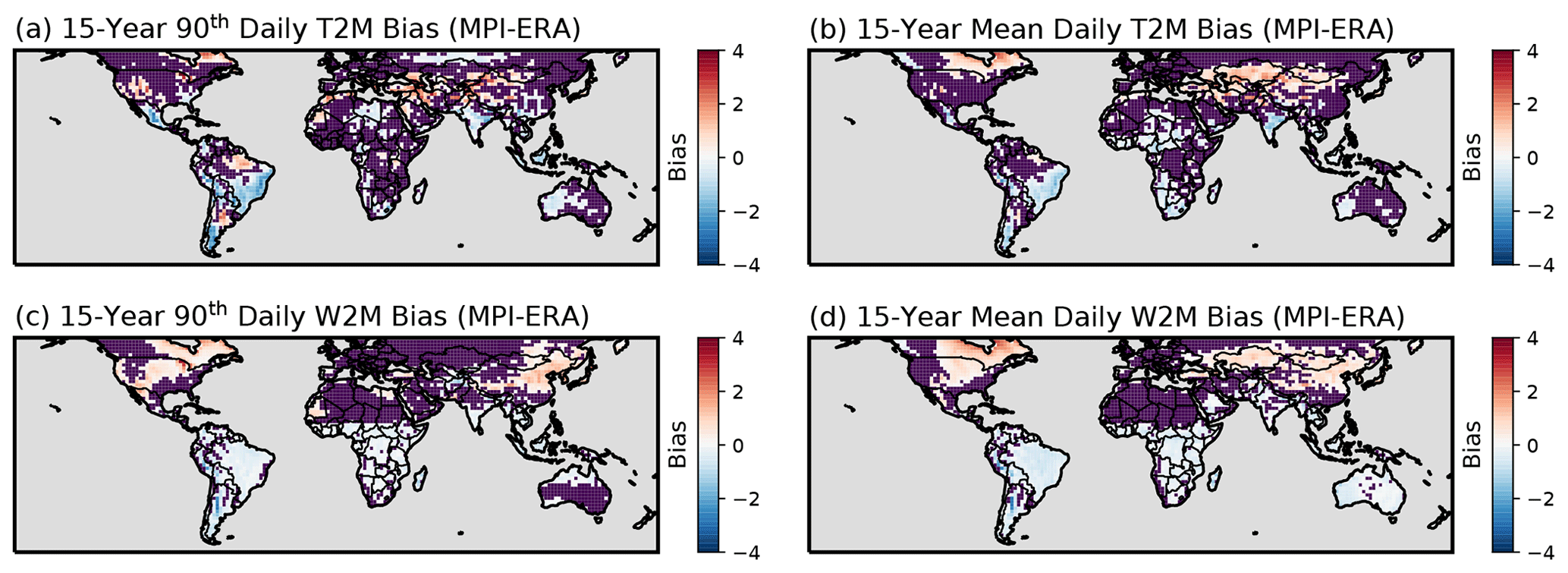
Figure 1Difference of 1 % CO2 runs compared with ERA-Interim in the same level of global warming (0.87 ∘C). The grid points where ERA-Interim falls within the ensemble spread of 1 % runs are masked with gray, while other grid points show the difference between the nearest ensemble member and ERA-Interim for the (a) 90th percentile of the 15-year daily average t2m, (b) the mean of 15-year daily average t2m, the (c) 90th percentile of 15-year daily average w2m, and (d) the mean of 15-year daily average w2m.
Generally, the 1 % runs overpredict t2m and w2m in Northern Hemisphere (NH) and underpredict in Southern Hemisphere (SH), except for India. This difference is consistent with the fact that the 1 % models do not contain aerosol forcing, which should lead to biases of the sign seen in Fig. 1. The w2m shows a larger area of differences than t2m, which suggests that there are larger biases in the dew point, which is needed in the calculation (Davies-Jones, 2008). The area-weighted averages of these differences are −0.08, −0.03, −0.04, and −0.11 ∘C globally for 90th percentile t2m, mean t2m, 90th percentile w2m, and mean w2m, respectively, which means that the model is, on average, underpredicting land temperature. Breaking down to the Northern and Southern hemispheres, the bias is 0.20, 0.21, 0.15, and 0.14 ∘C in the NH and −0.64, −0.54, −0.36, and −0.44 ∘C in the SH, confirming that the model is overpredicting land temperature in the NH and underpredicting land temperature in the SH.
To quantify the impact of the biases in Fig. 1 on the occurrence of heat extremes, we will perform sensitivity tests on the calculations by adding to each grid point of each member of the ensemble the average differences between the ensemble average t2m and w2m and the reanalysis. By evaluating how much our results change, we come up with an estimate of the impact of model biases on our results. As we will show later, these biases have little impact on the results of the paper.
2.2 Global population and GDP per capita data
Global population data from the NASA Socioeconomic Data and Applications Center (SEDAC, 2018) are used to weight the heat wave indices by population. The data represent the population in the year 2015 at 30×30 latitude–longitude spatial resolution, and we regridded this to the grid of the MPI model by summing the values in grid boxes surrounding the MPI grid centers. In our population-weighted calculations, we assume that the relative distribution of population remains fixed into the future.
Gridded GDP per capita data (Kummu et al., 2019) between 1990 and 2015 are used to estimate the risk of heat extreme events for different levels of wealth. These data are regridded from the original 5×5 latitude–longitude spatial resolution to the MPI model's resolution of by averaging the GDP inside the grid box. When doing this average, per capita GDP was weighted by population and also averaged over the 1990–2015 period. We assume that the relative percentile of GDP per capita for each grid point is fixed into the future, so changes in climate risk are due to exposure to warmer climate extremes and not changes in relative per capita wealth.
3.1 Global warming
Global warming is defined as the global and annual average temperature increase compared to the average of first 5 years of the 1 % run. We find that ensemble and global average t2m reaches 1.5, 2, 3 and 4 ∘C in years 59, 76, 108, and 133, respectively, and reaches 4.6 ∘C at the end of the 150-year run. The increase in the global average temperature is nearly linear for both t2m and w2m, consistent with a linear ramping of the forcing (Buzan and Huber, 2020).
The focus of the paper will be on heat extremes at 1.5, 2 and 3 ∘C. The 1.5 and 2 ∘C thresholds are the limits described in the Paris Agreement, while 3 ∘C is the warming we are presently on track for (Hausfather and Peters, 2020).
3.2 Heat wave indices
Identification of heat waves is done in several steps. First, for each grid point, we smooth a daily maximum temperature (determined form 6 h temperatures) using a 15 d moving window for the first 5 years of 1 % runs, which is the period before significant warming has occurred. Then, the 90th percentile of the smoothed daily maximum temperature for the first 5 years was calculated at each grid point (Fischer and Schär, 2010). This value is used as a threshold for the heat waves at that grid point. Then we calculate the heat wave days, defined as days that exceed the threshold for 3 or more consecutive days (Baldwin et al., 2019).
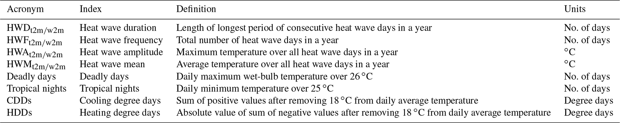
We then define four indices to represent the characteristics of these heat waves. To determine the occurrence of events, the heat wave duration (HWD; longest heat wave of the year) and heat wave frequency (HWF; total number of heat wave days in a year) are calculated. From an intensity perspective, the heat wave amplitude (HWA; maximum temperature during heat wave days during a year) and heat wave mean (HWM; mean temperature during heat wave days in a year) are selected. These indices are also calculated in an analogous fashion for the wet-bulb temperature (w2m), since the wet bulb temperature is arguably more relevant for human health (Heo et al., 2019; Morris et al., 2019; Buzan and Huber, 2020). These indices are summarized in Table 1.
3.3 Deadly days and tropical nights
Heat wave thresholds are different for each grid point because they are based on preindustrial temperatures at that grid point. Combined with regional differences in the ability to adapt, this means that heat waves in different regions may have different implications for human society. We, therefore, also count the number of days in each year with daily maximum w2m above 26 ∘C, which we refer to as “deadly days”. We note that other values could be chosen (Liang et al., 2011), with higher values occurring less frequently but with more significant impacts. This value is based on the analysis of Mora et al. (2017), who demonstrated that a w2m of about 24 ∘C is the threshold at which fatalities from heat-related illness occur. However, since we find that there are some regions that already experience over 9 months of 24 ∘C w2m events per year, we increase this threshold to 26 ∘C in our analysis. We could have chosen higher w2m values, but any choice in this range is associated with negative impacts, so we have chosen a value near the bottom of the range where mortality occurs in order to maximize the signal in the model runs.
A warm nighttime minimum temperature can be as important as a high maximum temperature for human health and mortality (Argaud et al., 2007; Patz et al., 2005), so we define “tropical nights” as a daily minimum t2m over 25 ∘C (Lelieveld et al., 2012).
3.4 Cooling degree days and heating degree days
To assess the economic and energy impact of heat extremes, cooling degree days (CDDs) and heating degree days (HDDs) are calculated. CDDs and HDDs are metrics of the energy demand to cool and heat buildings. For each grid point, the annual CDD is calculated by subtracting 18 ∘C from the daily average temperature and summing only the positive values over the year. The HDD is the absolute value of the sum of the negative values. Previous studies reported that CDDs and HDDs are closely related to energy consumption (Sailor and Muñoz, 1997).
4.1 Impact of unforced variability in climate on regional heat extremes
To investigate the impact of unforced variability in more regional heat extremes, we take the 15 largest cities by population (Fig. 2a) and determine the number of deadly days and tropical nights over time by averaging the 3×3 grid points surrounding the city and only including the land grid points. Figure 2b–d depict the ensemble-averaged number of deadly days and tropical nights, as well as the spread between the ensemble members. The error bars in Fig. 2b–d show the highest and lowest values of the extremes.
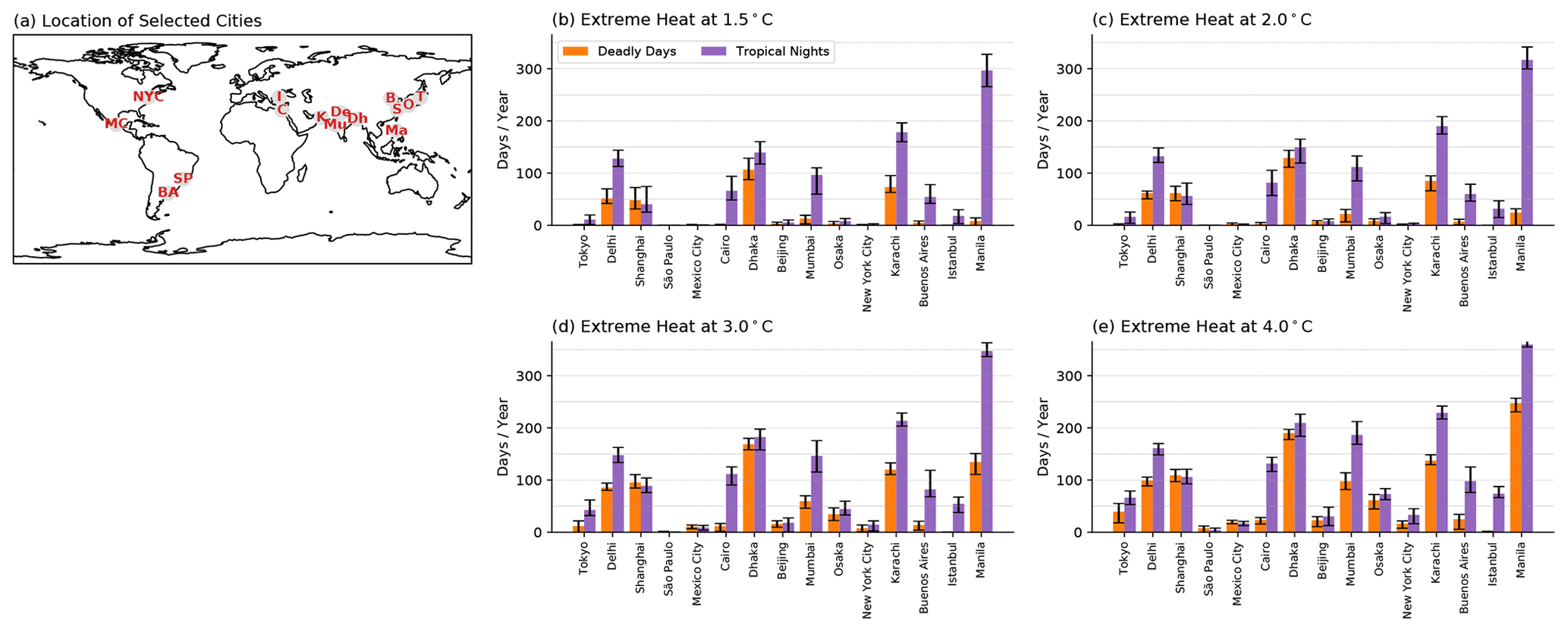
Figure 2(a) Location of 15 largest cities in the world and the number of annual heat extremes at (b) 1.5, (c) 2.0, (d) 3.0, and (e) 4.0 ∘C of global warming. Orange (purple) bars represent the ensemble average annual number of deadly days (tropical nights), averaged 5 years after each level of warming is exceeded. The number of heat extreme days are calculated by averaging a 3×3 land-only grid covering the selected city. Error bars represent the values of maximum and minimum ensemble members.
This difference within the ensemble is the result of unforced variability. For all 15 cities, the average spread in the number of deadly days at 1.5, 2.0, 3.0, and 4.0 ∘C of global warming between the ensemble members with maximum and minimum numbers is 14.3, 15.1, 20.6, and 21.9 d yr−1. For tropical nights, the spread is 29.3, 27.7, 29.1, and 26.7 d yr−1. So, on average, unforced variability can change the number of extreme days and nights by a few weeks per year. There is no significant variance of ensemble spread between the cities, except for cities with very low ensemble-averaged values (e.g., Mexico City at 1.5 ∘C warming) or very high values (e.g., tropical nights in Manila at 4.0 ∘C warming). However, for the cities that do not see a large increase in extreme temperatures (e.g., New York City), this represents a very large fraction of the predicted change of extremes, while for cities that experience a much larger increase (e.g., Manila), it represents a smaller percentage.
As discussed in Sect. 2.1, we examine the sensitivity of our results to potential biases of the model by recalculating the deadly days and tropical nights using model data after adding in the bias estimated by a comparison to the reanalysis. The average difference of deadly days in the sensitivity test (absolute difference) at 1.5, 2.0, 3.0, and 4.0 ∘C warming is 2.1, 2.5, 5,5, and 7.6 d yr−1 when averaged over 15 cities. The standard deviation of the difference calculated between the cities is 2.5, 3.4, 6.7, and 9.7 d at each level of warming. For tropical nights, sensitivity test produced differences of 3.6, 3.6, 5.3, and 3.5 d yr−1 at each level of warming, with standard deviations within the ensemble of 3.6, 4.9, 6.9, and 1.8 d. Thus, model biases are unlikely to have a large impact on our results.
Previous work has attempted to distinguish the origin and mechanisms of unforced variability in temperature and temperature extremes (Meehl et al., 2007; Zhang et al., 2020; Birk et al., 2010). To probe the statistical modes of variability affecting this ensemble spread and to identify the underlying physical mechanisms, an empirical orthogonal function (EOF) analysis (North, 1984) was performed on the detrended and normalized time series of deadly days and tropical nights for the 15 cities. For each city, the 28 ensemble members are concatenated together (total of 28×150 years) in order for all ensembles to share the same EOF. In this way, we aim to find the dominant drivers of unforced variability that impacts heat extremes in the largest cities around the world.
The first three EOF patterns for each city are plotted in Fig. 3 as bars. The first EOF mode of deadly days shows large values for Delhi, Shanghai, Dhaka, and Karachi, while cities in other regions show lower values. The second and third EOFs for deadly days show more variability between the cities. The first EOF for tropical nights (Fig. 3d) shows large positive values for cities in the India–Pakistan region, with other cities showing smaller magnitude changes. The second EOF shows large negative values in Cairo, Istanbul, and Manila, while the third EOF for tropical nights shows more variability between the cities.
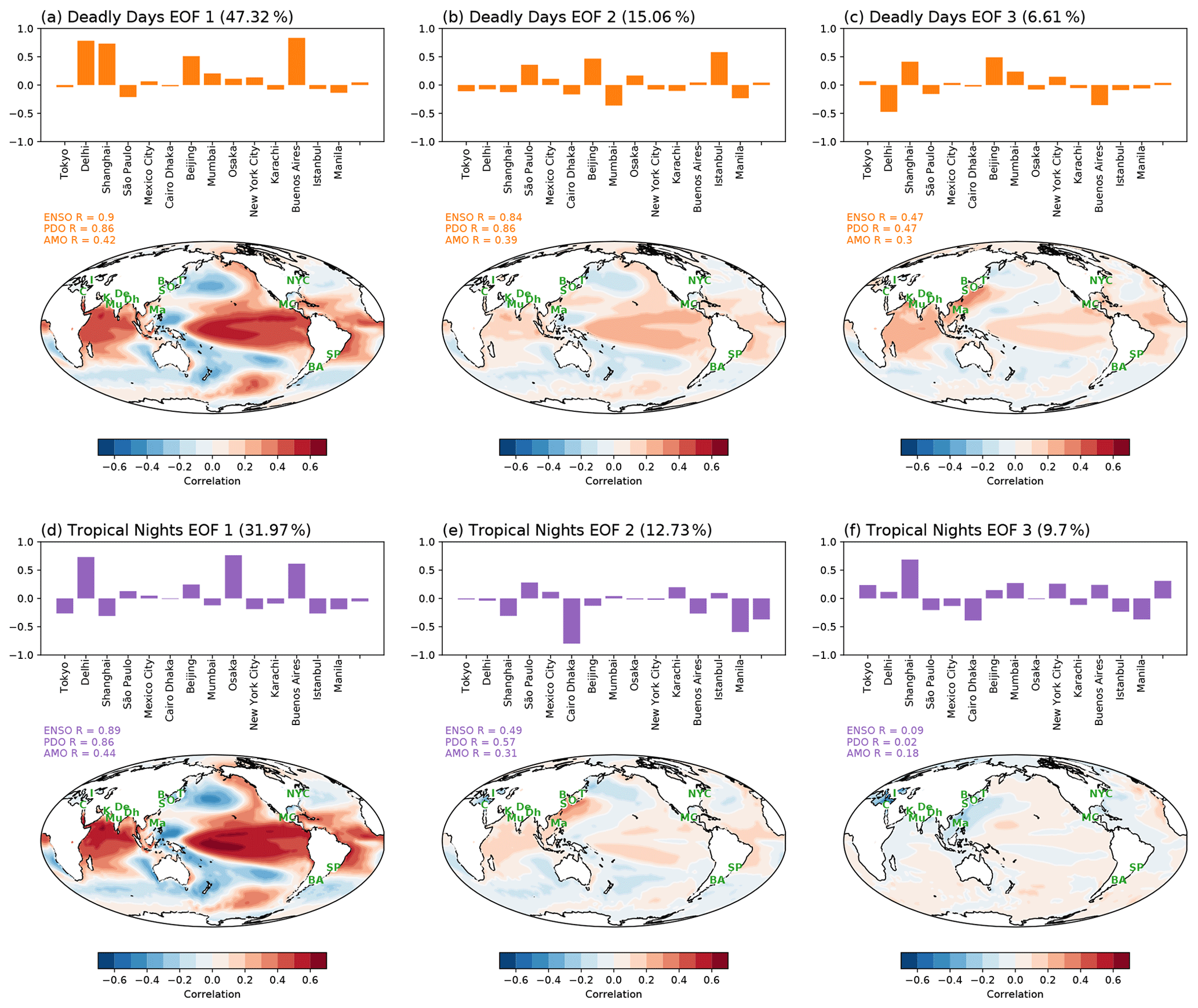
Figure 3The first three EOFs of annual values of deadly days (a–c) and tropical nights (d–f) in the world's 15 largest cities. For each panel, the bar graph shows the EOF pattern of the number of heat extreme days per year. Contour plots shows the SST pattern associated with the EOF mode, obtained by projecting each mode of PC onto SST anomalies. Ensemble members are averaged to yield the SST pattern. Pattern correlations with major modes of climate variability (ENSO, PDO, and AMO) are also shown, as discussed in the text.
The PC (principal component) time series are projected onto detrended annual sea surface temperature (SST) anomalies. This allows us to investigate how heat extreme events in 15 major cities are associated with global modes of unforced variability. Maps of correlation coefficients are also plotted in Fig. 3. Characteristic patterns for ENSO (Trenberth and National Center for Atmospheric Research Staff, 2020), PDO (Deser et al., 2016), and AMO (Trenberth et al., 2020) are calculated for each ensemble using all 150-years of SSTs, and the pattern is averaged over the ensembles to come up with a single ENSO, PDO, and AMO SST pattern for the ensemble. Then, those patterns are compared with the PC projection on SST to see how PC-projected SSTs resemble the patterns of unforced variability. Correlation coefficients between the standard climate indices and PC-projected SST is shown in the lower panel of Fig. 3 as numbers. All of the projections of deadly day PCs and projections of the first two modes of tropical nights show patterns similar to ENSO and PDO.
Power spectra of the PCs are calculated individually for each ensemble member, and then the ensemble average is plotted Fig. 4. Overall, the spectra of the deadly day PCs look very much like the spectrum for ENSO, and it notably does not have the ∼20-year peak of the PDO spectrum. This tells us that, in this model at least, the variability in the occurrence of deadly days in these large cities is strongly regulated by ENSO. This may be a consequence of the fact that these large cities are mostly located near the ocean and at lower latitudes. The third deadly day PC has lower correlations with the ENSO or PDO indexes, so it is harder to draw firm conclusions about the mechanism behind it. Also, higher modes of EOFs are unlikely to refer to a single mode of climate due to the orthogonality constraints between each mode. The tropical night PCs also show peaks at ENSO periods (Fig. 4b) suggesting that, like deadly days, tropical night variability is controlled by ENSO.
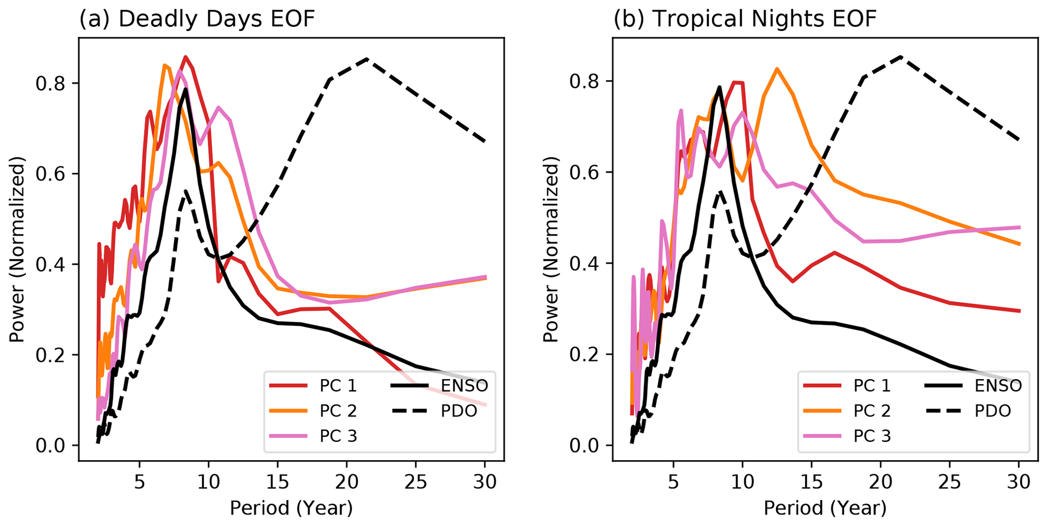
Figure 4Frequency power spectrum of ENSO, PDO, and PC of the first three EOF modes for (a) deadly days and (b) tropical nights. ENSO is calculated with the Niño 3.4 index, and PDO is calculated as a leading EOF of SST anomaly in the North Pacific basin. Monthly SST data are used for both ENSO and PDO, and then each index is averaged over the year to have consistency with deadly days and tropical nights.

Figure 5(a) Clustered regions via K-means clustering. Characteristics of each cluster are listed in Table 2. (b) Zonal average of temperature increases at the time of 0.87 (our reference period), 1.5, 2, and 4 ∘C of global warming compared to the preindustrial baseline in the 1 % runs. Temperatures are averaged over a 5-year period after each warming threshold is exceed in the model.
4.2 Cluster analysis and population risk of heat wave indices
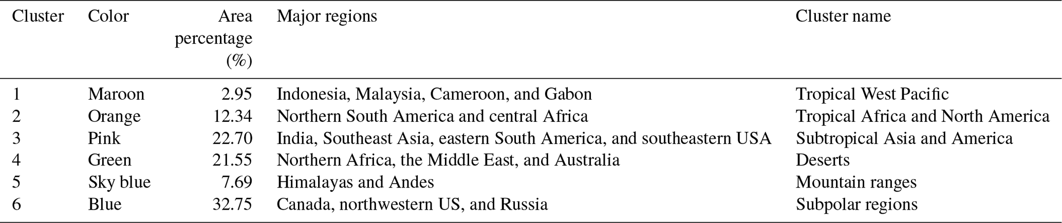
We calculate HWD, HWF, HWA, and HWM for both t2m and w2m each year at each grid point, which generates eight different 150-year time series for each of the 28 ensemble members. Each time series at each grid point is regressed vs. time, yielding a slope and the intercept for each time series in all 28 ensemble members. The 16 variables (8 heat wave indices × 2 slope and intercept) are then utilized as a predictor variable for K-means clustering (Likas et al., 2003) to categorize the spatial variation in heat waves using the Euclidean distance of its predictor variables (16 variables). With slope and intercept, we can characterize the heat indices of each grid point with response to CO2 forcing (slope) and climatology (intercept). The number of clusters in this study is set to 6, using the elbow method (Syakur et al., 2018). When using five clusters, we find that two clusters (the light and dark blue regions in Fig. 5a) merge, and when using seven clusters, we find that one cluster (the dark blue region in Fig. 5a) divides into two separate clusters.
Figure 5a shows the cluster value that most ensembles assigned to each grid point, and it shows distinct geographical characteristics, as summarized in Table 2 (the result of clustering shows little difference between individual ensemble members). As might be expected from how we calculated the 16 variables for clustering, each cluster shows a different evolution of heat extremes in a warmer world (Fig. 6). Although the warming signal is the largest in the polar regions (Fig. 5b), the largest increases in HWD and HWF are found at lower latitudes (in cluster 1 and 2 in Fig. 6a–d). This is mostly due to low variability in these regions compared to polar regions, making it easier for a trend to exceed the heat wave threshold.
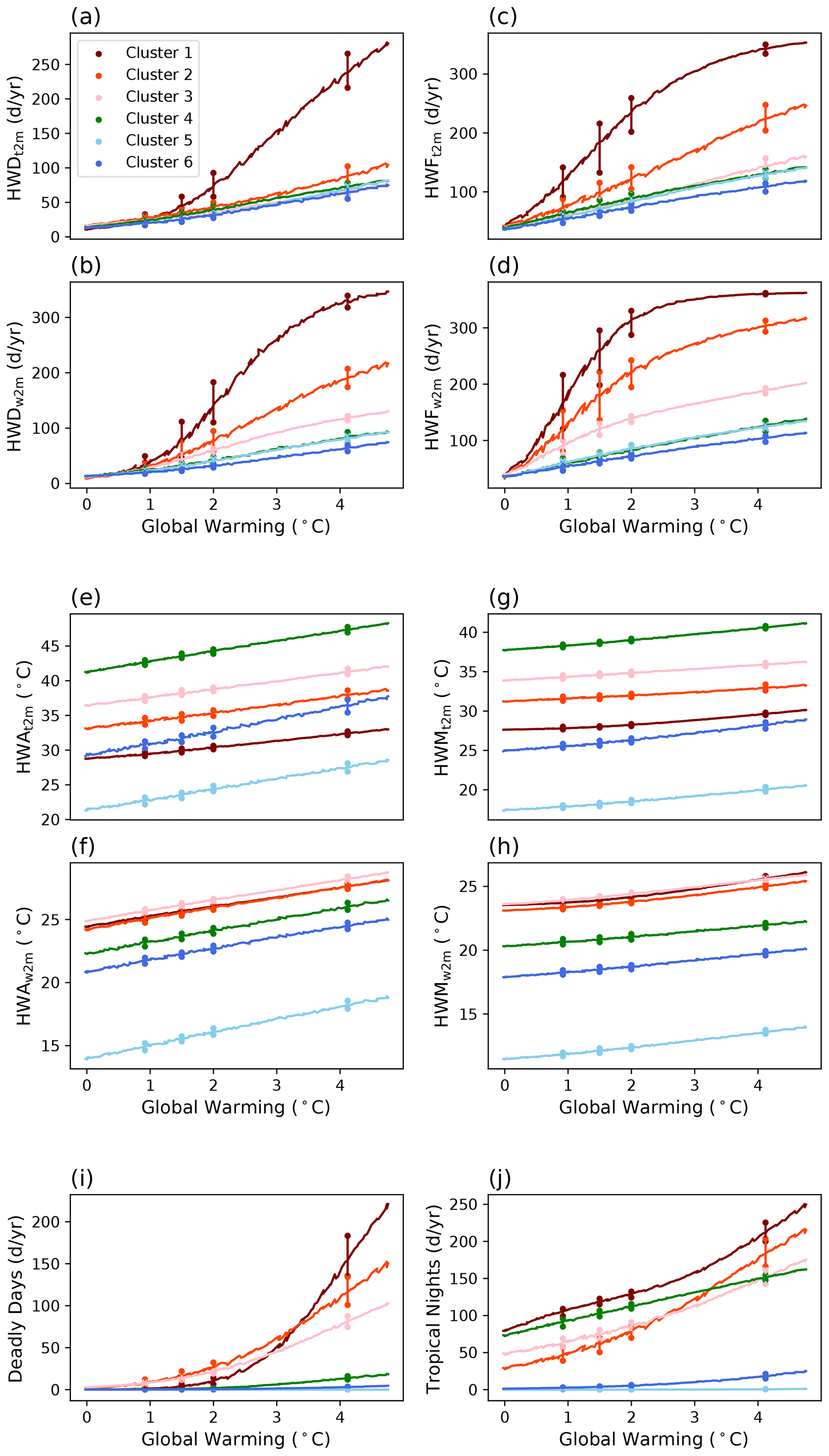
Figure 6Evolution of each index averaged over each cluster. Colors are consistent with Fig. 5 and Table 2. The values of each metric are calculated by averaging the grid points that belong to each cluster. This was done for each ensemble member, and then the ensemble average is plotted. Vertical lines with dots show the maximum and minimum of 28 ensemble members at each threshold of warming to represent the spread between the ensemble members.
Table 2Percentage area and major regions belonging to each cluster. Clusters are identified only for the global land areas.
These results are insensitive to potential model biases. Sensitivity tests show that adding the bias to the model changes HWD, HWF, deadly days, and tropical nights by less than 5 % for all metrics and clusters. For HWA and HWM, the difference caused by adding the bias was less than 1 ∘C for all metrics and clusters, suggesting that the impact of model biases is small in this analysis.
For HWA and HWM, the rate of increase is similar for all clusters, with increases in HWAt2m and HWAw2m of 1.45 ∘C per degree of global average warming, respectively, and HWMt2m 0.85 ∘C per degree of global average warming, respectively, and HWMt2m and HWMw2m of 0.66 ∘C per degree of global average warming and 0.47 ∘C per degree of global average warming, respectively (Fig. 6e–h). The exception is HWAt2m in cluster 6. The large increase in HWAt2m in this region is connected to the strong global warming signal in high latitudes that has been predicted for decades and is now observed (Stouffer and Manabe, 2017).
Turning to deadly days (Fig. 6i), we find that a substantial increase occurs in cluster 1 after 2.0 ∘C of warming; this is important because it gives additional support for the Paris Agreement's aspirational goal of limiting global warming to 2.0 ∘C. Almost all increases in deadly days are in low latitudes (clusters 1, 2, and 3). For tropical nights, low latitudes and deserts (cluster 4) contribute most of the increase. Figure 6 also shows the spread within the ensemble for each metric and cluster. We find that the spread for a cluster is generally small compared to the change over time and the difference between the clusters.
We also generated indices weighted by global population. Heat wave indices for the 95th percentile of population (meaning 5 % of the population is exposed to higher values), the 90th percentile of population, and the median of the population are depicted in Fig. 7. Figure 7a shows that, with 3 ∘C of warming, 5 % of the Earth's population will experience heat waves lasting 122 d (standard deviation between ensemble members of 1σ=17 d), 10 % of the population will experience heat waves lasting 94 d (1σ=7 d), and half of the population will experience heat waves lasting around 50 d (1σ=4 d). These are large increases over present-day values of 50, 42, and 21 d. The average of the standard deviation between the ensemble members (calculated every year and then averaged) is 10.6, 6.2, and 3.7 d for the 95th, 90th percentile, and median, respectively. This is significantly smaller than the values from the analyses of the cities in Fig. 2, where the unforced variability makes larger differences in the occurrence of heat waves.

Figure 7Changes in population-weighted heat wave indices as a function of global average warming. Each line denotes one ensemble member for different percentiles of the population.
The rate of increase in HWFw2m in Fig. 7d shows a rapid increase until the global average warming reaches about 2.5 ∘C. Given that the planet has already warmed about 1 ∘C above preindustrial levels, this suggests that the world should presently be experiencing a rapid increase in wet bulb extreme frequency, particularly in the tropics. This is related to the increased slope in Fig. 6, in which values of HWDw2m and HWFw2m for clusters 1 and 2 increase rapidly until 3.0 and 2.0 ∘C of global warming. At warmer temperatures, HWDw2m and HWFw2m reach a plateau, since values over 300 d yr−1 mean there is little room for additional increases. For HWA and HWM, the increase is mostly linear. Also note that, at 3 ∘C of global warming, the 90th percentile of population-weighted HWAw2m reaches over 29 ∘C, which, while not immediately fatal to humans, may, nevertheless, indicate great difficulty for even a developed society to adapt to.
Currently, 10 % of the total population faces more than 45 deadly days and 181 tropical nights per year. This grows to 65 and 195 d, respectively, at 1.5 ∘C warming. With 2 ∘C of global warming, 10 % of the population will face about 3 months of deadly days and 7 months of tropical nights every year, and this increases to 4 and 8 months with 3 ∘C of warming. Also, with 3 ∘C of global warming, 5 % of the population will be in an environment where 8 and 10 months a year are deadly days and tropical nights. Our sensitivity tests suggest that model bias generates less than 5 % differences for HWD, HWF, deadly days, and tropical nights for all metrics and the percentile of population at every level of global warming, except when the metrics are near zero. Potential model biases also generate small differences in HWA and HWM, with less than 1 ∘C difference in all metrics for every period. Furthermore, with 3 ∘C of global warming, the minimum ensemble member of deadly days is above the maximum ensemble of the present-day reference (0.87 ∘C) for all population percentiles (5 %, 10 %, and 50 %). This occurs at 2 ∘C for tropical nights. Details of the ensemble spread are also shown in Table 3.
Table 3Number of deadly days each percentile (p.) of the global population faces, with reference period (0.87 ∘C) and 1.5, 2, 3, and 4 ∘C of global warming from the preindustrial condition. Standard deviations between the ensembles (1σ) are also shown.
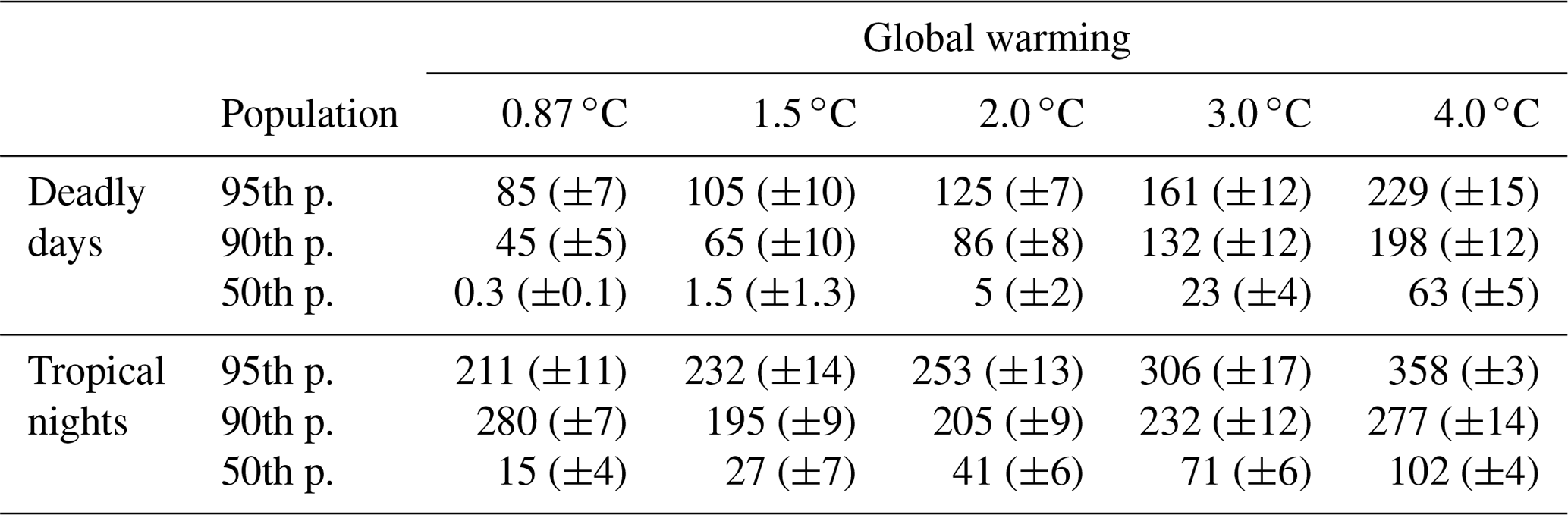
It is notable that, although there is a large spread between the ensemble members in each city (Fig. 2), the spread in the clusters (Fig. 6) and population-weighted metrics (Fig. 7) is not as large. This emphasizes that the effect of unforced variability might be large at small scales, but as the region expands, the impact of unforced variability decreases. This is also found in Table 3, where, in each case, the standard deviation between ensembles is less than 20 % of the average, except in a few cases. This indicates that unforced variability will generally play a minor role in determining global exposure to temperature above thresholds, although different people may be affected in different realizations of unforced variability.
In addition, with 1.5 ∘C of global warming, the lowest ensemble of the 90th percentile of HWDt2m, HWDw2m, and HWFt2m exceeds the highest ensemble of the same metric in the current climate (red lines in Fig. 7). With 2 ∘C of warming, the minimum ensemble of HWD, HWF, HWMw2m, and tropical nights exceed the maximum ensemble of the current climate, and with 2.5 ∘C of warming, the minimum ensemble of all metrics exceeds the maximum ensemble of the same metric in the current climate. Thus, this model predicts that the occurrence of extremes will soon be able to exceed values likely possible in our present climate for these metrics.
4.3 Analysis on GDP per capita
It is well known that not everyone is equally vulnerable to extreme weather, with rich, relatively more developed communities having more resources to deal with extreme events than poorer communities. In that context, the global gridded GDP per capita is used to calculate average risk at each level of wealth. The ensemble-averaged result is depicted in Fig. 8, which shows the absolute number of deadly days and tropical nights, as well as the increase in the number of deadly days and tropical nights that each economic level experiences relative to the reference period warming of 0.87 ∘C. This plot assumes that the relative distribution of population and GDP remains fixed through time. Our sensitivity tests show that the model bias yields small differences in the results, with less than 5 % difference in both the absolute number of extreme events and the changes in extremes.
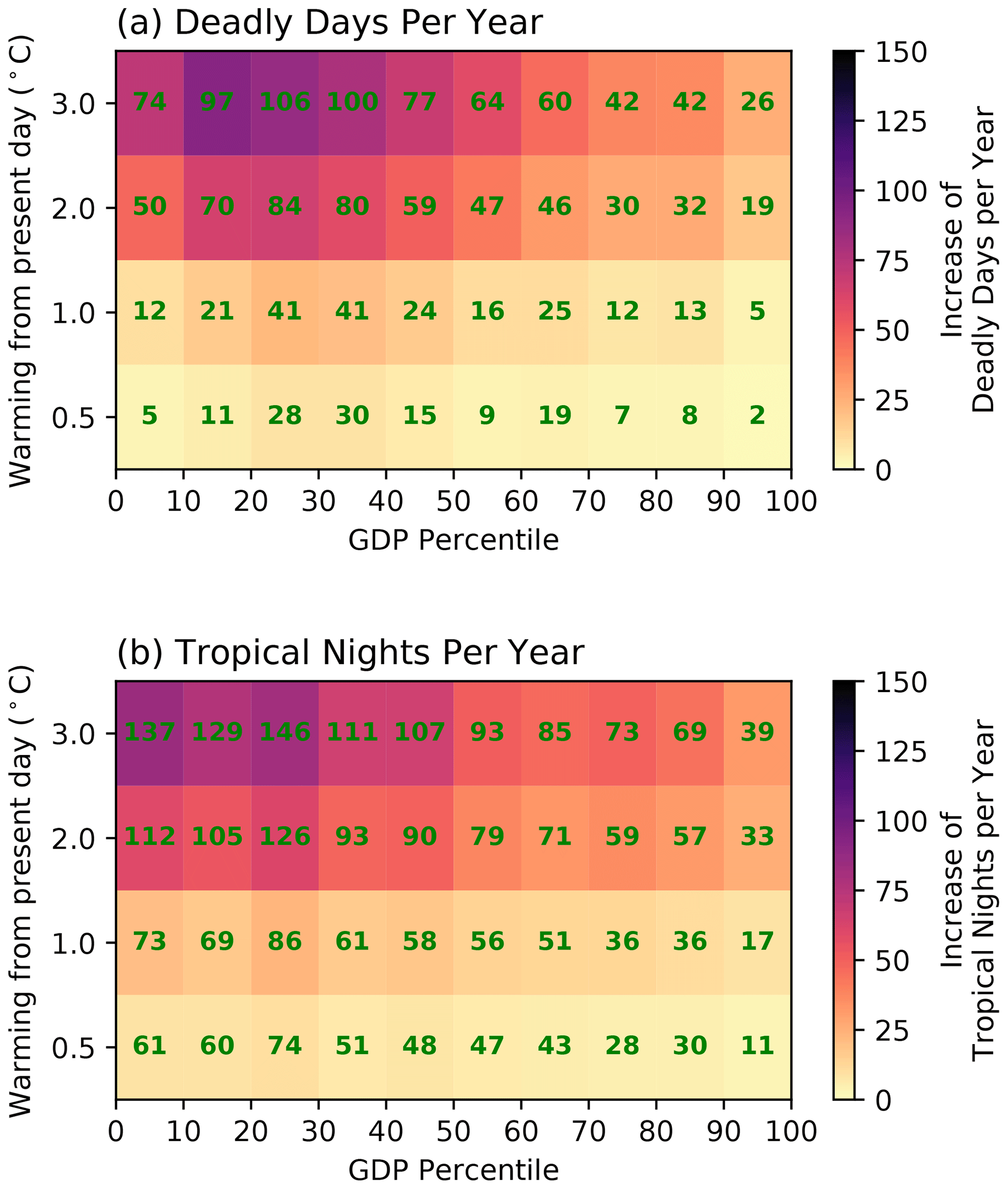
Figure 8Increase in (a) deadly days and (b) tropical nights compared to the reference period (0.87 ∘C of warming), binned by the percentile of GDP per capita at selected levels of warming compared to reference climate (calculated by subtracting reference values, shown as a heat map), averaged over the population within the GDP percentile (for example, averaged over population in 0–10 percentile of GDP) and over all ensemble members for 5-year window after each level of warming first occurs. Green text inside the heat map represents the absolute number of deadly days and tropical nights in each level of warming.
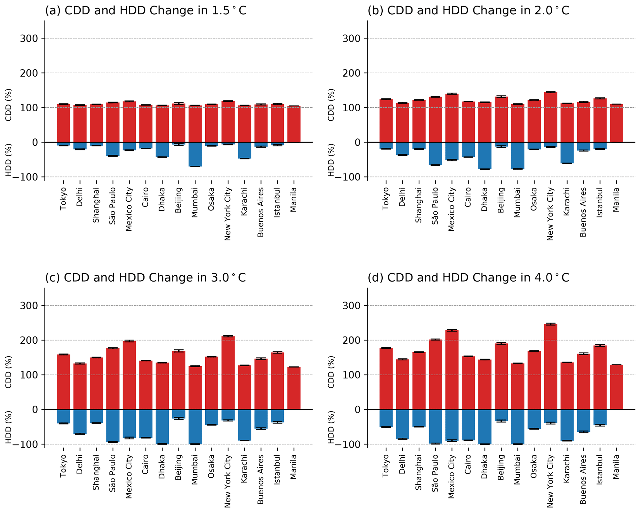
Figure 9Change (in percentage) of ensemble-averaged cooling degree days (CDD; red) and heating degree days (HDD; blue) compared to the reference climate (0.87 ∘C) in the 1 % CO2 experiments at the time they reach the global mean temperature thresholds of (a) 1.5 ∘C, (b) 2.0 ∘C, (c) 3.0 ∘C, and (d) 4.0 ∘C, respectively. Error bars represent the standard deviation in CDD and HDD values between the ensemble members.
For each level of warming, we find that the lower GDP regions will experience not only higher absolute numbers of extreme temperature days but also the largest increases. For deadly days, the increase is largest between 10th to 40th percentile of GDP, and for tropical nights, the increase is largest below the 30th percentile of GDP. The regions that contribute the most for the low GDP percentiles are in Southeast Asia, including Myanmar, Laos, and Cambodia, and tropical Africa, including the Democratic Republic of the Congo, Kenya, Uganda, Ethiopia, and the Republic of Sudan, which are in clusters 1 and 2 in our cluster analysis (Fig. 5). The maximum difference in heat wave days between the ensembles is less than 25 % for all GDP and global warming levels.
4.4 Energy demand on large cities
Annual CDDs and HDDs have been calculated for the 15 cities in Sect. 4.1. Both CDDs and HDDs are calculated by averaging the CDD and HDD values of 3×3 grid points surrounding each city, including only land grid points. CDD and HDD values are then averaged for 5 years after global warming reaches each levels of threshold. Figure 9 shows the percent change in CDDs and HDDs at 1.5, 2.0, 3.0, and 4.0 ∘C relative to the reference period CDD and HDD values. This was done for each city and for each ensemble member. At 1.5, 2.0, 3.0, and 4.0 ∘C warming, CDDs in the 15 cities increase by an average of 9 %, 22 %, 54 %, and 70 %. Our sensitivity tests show that the application of the average model bias yields changes of less than 1 % in these numbers. This suggests an enormous increase in energy required for cooling.
In contrast, average energy demand on cold days (HDDs) decreases by 21 %, 36 %, 59 %, and 65 % in cities considered, compared to present day, partially offsetting the increase in energy required for cooling. Manila shows 0 % change in HDDs for all periods, since Manila does not experience HDD days in present or future periods. Sensitivity tests also show less than a 1 % difference in HDD change due to model biases.
In this study, we found that extreme heat events will become more frequent and severe in a warming world. We find that both forced and unforced variability play a key role in extreme heat events, highlighting the necessity of considering both contributions to extreme heat. We also look at population-weighted and GDP-sorted statistics of extreme heat in warmer world.
Our results show that ENSO is the dominant mode of unforced variability impacting the occurrence of extreme heat and humidity events and that events tend to be synchronous in the world's largest 15 cities. But while the impact of unforced variability might be significant regionally and temporarily, it becomes less important when one looks at larger aggregate regions.
Looking at global population-weighted statistics, we found that, with 1.5 ∘C of global average warming, over 10 % of the population will face heat waves of 45 ∘C temperature and 28 ∘C wet-bulb temperatures. Furthermore, 5 % of the population will face more than 105 d of deadly days and 232 d of tropical nights per year. With 3 ∘C of warming, which we are currently on track for, 10 % of the population will experience over 132 d of deadly days and over 232 d of tropical nights per year. Moreover, 10 % of the population will face a 47 ∘C temperature and 30 ∘C wet-bulb temperature. Given that these two metrics have important implications for human mortality, such increases may have significant impacts on human health globally.
Sorting heat and humidity events by wealth, we confirm that the increasing frequency and severity of extreme events will fall mostly on poorer people. To further investigate some economic impacts of increasing heat extremes, cooling degree days (CDDs) and heating degree days (HDDs) are calculated for the world's 15 largest cities. Energy demand for cooling (CDDs) increases by an average of 9 % for 1.5 ∘C and 54 % for 3.0 ∘C of warming, while energy demand for heating (HDDs) decreases by 21 % and 59 %. Since CDDs are known to have a piecewise linear relationship with the energy consumption, with the slope increasing with higher CDDs (De Rosa et al., 2014; Shin and Do, 2016), increasing CDDs in a warmer world could be one of the factors driving increased economic inequity from global-warming-related heat extremes, due to relatively high costs and the need for energy in the poorest countries.
Uncertainties in this analysis include our use of gridded 6 h climate model output. More detailed analysis could be done with climate simulations with higher temporal and spatial resolution. The model has biases relative to measurements, potentially due to the fact that there are no aerosols in the forcing, which is another source of uncertainty. This was tested by adding the difference between the ensemble average and the reanalysis data to the model fields and recomputing the heat wave indices. In general, the impact of this bias was not important. In future analyses, this could be better resolved with use of multimodel ensembles or detailed bias correction of the model.
Another uncertainty is that our runs are continuously warming, and it is possible that an equilibrium world at any given temperature may experience a different occurrence of extremes than in the runs in this paper. Additionally, since an increasing proportion of the population is expected to live in dense metropolitan areas, there is also the possibility that actual heat and humidity extremes that populations experience could be more severe than the gridded data due to local phenomena such as the urban heat island effect (Murata et al., 2012). Statistical or dynamical downscaling could be used for a more detailed analysis (Dibike and Coulibaly, 2006; Wood et al., 2004). Also, land models with the capacity to decompose the urban and rural environment could be applied in the same context (Bonan et al., 2002; Dickinson et al., 2006). Also, this study could gain further insights by considering changing population and socioeconomic distribution in the future. Overall, however, none of these things are expected to change the broad conclusion of this study that global warming will lead to increased exposure to extremes in heat and humidity.
The 6 h 1 % runs from MPI–GE can be distributed upon request. ERA-Interim data are available from the ECMWF archive (https://www.ecmwf.int/en/forecasts/datasets/reanalysis-datasets/era-interim, last access: October 2018) (Berrisford et al., 2018). Global population data are available from the NASA SEDAC archive (https://doi.org/10.7927/H49C6VHW) (CIESIN, 2020). Global GDP per capita can be obtained from Kummu et al. (2019) (https://doi.org/10.5061/dryad.dk1j0).
JL, JM, and AD conceptualized the project. The data curation was done by JL and AD, while JL and JM conducted the formal analysis. AD acquired the funding, while JL and JM led the investigation. JL took responsibility for the methodology, software, and visualization. AD administered and supervised the project and acquired the resources. JL and AD wrote the paper.
The authors declare that they have no conflict of interest.
Publisher's note: Copernicus Publications remains neutral with regard to jurisdictional claims in published maps and institutional affiliations.
This research has been supported by the Division of Atmospheric and Geospace Sciences (grant nos. AGS-1661861 and AGS-1841308) to Texas A & M University.
This paper was edited by Mathias Palm and reviewed by Sabine Undorf and one anonymous referee.
Arbuthnott, K., Hajat, S., Heaviside, C., and Vardoulakis, S.: Changes in population susceptibility to heat and cold over time: assessing adaptation to climate change, Environ. Health, 15, 73–93, 2016.
Argaud, L., Ferry, T., Le, Q. H., Marfisi, A., Ciorba, D., Achache, P., Ducluzeau, R., and Robert, D.: Short- and long-term outcomes of heatstroke following the 2003 heat wave in Lyon, France, Arch. Intern. Med., 167, 2177–2183, https://doi.org/10.1001/archinte.167.20.ioi70147, 2007.
Baldwin, J. W., Dessy, J. B., Vecchi, G. A., and Oppenheimer, M.: Temporally Compound Heat Wave Events and Global Warming: An Emerging Hazard, Earths Future, 7, 411–427, https://doi.org/10.1029/2018ef000989, 2019.
Berrisford, P., Dee, D., Poli, P., Brugge, R., Fielding, K., Fuentes, M., and Simmons, A.: The ERA-Interim archive Version 2.0, Shinfield Park, Reading, available at: https://www.ecmwf.int/en/forecasts/datasets/reanalysis-datasets/era-interim, last access: October 2018.
Birk, K., Lupo, A. R., Guinan, P., and Barbieri, C.: The interannual variability of midwestern temperatures and precipitation as related to the ENSO and PDO, Atmosfera, 23, 95–128, 2010.
Bonan, G. B., Oleson, K. W., Vertenstein, M., Levis, S., Zeng, X., Dai, Y., Dickinson, R. E., and Yang, Z.-L.: The land surface climatology of the Community Land Model coupled to the NCAR Community Climate Model, J. Climate, 15, 3123–3149, 2002.
Buzan, J. R. and Huber, M.: Moist heat stress on a hotter Earth, Annu. Rev. Earth Planet. Sci., 48, 623–655, https://doi.org/10.1146/annurev-earth-053018-060100, 2020.
Buzan, J. R., Oleson, K., and Huber, M.: Implementation and comparison of a suite of heat stress metrics within the Community Land Model version 4.5, Geosci. Model Dev., 8, 151–170, https://doi.org/10.5194/gmd-8-151-2015, 2015.
Chen, R. D. and Lu, R. Y.: Dry Tropical Nights and Wet Extreme Heat in Beijing: Atypical Configurations between High Temperature and Humidity, Mon. Weather Rev., 142, 1792–1802, https://doi.org/10.1175/Mwr-D-13-00289.1, 2014.
Chow, W. T., Chuang, W.-C., and Gober, P.: Vulnerability to extreme heat in metropolitan Phoenix: spatial, temporal, and demographic dimensions, Profess. Geogr., 64, 286–302, 2012.
CIESIN – Center for International Earth Science Information Network: Columbia University Gridded Population of the World, Version 4 (GPWv4): Population Density, Revision 11, NASA Socioeconomic Data and Applications Center (SEDAC), [data set], https://doi.org/10.7927/H49C6VHW, 2020.
Dahl, K., Licker, R., Abatzoglou, J. T., and Declet-Barreto, J.: Increased frequency of and population exposure to extreme heat index days in the United States during the 21st century, Environ. Res. Commun., 1, 075002, https://doi.org/10.1088/2515-7620/ab27cf, 2019.
Davies-Jones, R.: An efficient and accurate method for computing the wet-bulb temperature along pseudoadiabats, Mon. Weather Rev., 136, 2764–2785, 2008.
Dee, D. P., Uppala, S. M., Simmons, A. J., Berrisford, P., Poli, P., Kobayashi, S., Andrae, U., Balmaseda, M. A., Balsamo, G., Bauer, P., Bechtold, P., Beljaars, A. C. M., van de Berg, L., Bidlot, J., Bormann, N., Delsol, C., Dragani, R., Fuentes, M., Geer, A. J., Haimberger, L., Healy, S. B., Hersbach, H., Holm, E. V., Isaksen, L., Kallberg, P., Kohler, M., Matricardi, M., McNally, A. P., Monge-Sanz, B. M., Morcrette, J. J., Park, B. K., Peubey, C., de Rosnay, P., Tavolato, C., Thepaut, J. N., and Vitart, F.: The ERA-Interim reanalysis: configuration and performance of the data assimilation system, Q. J. Roy. Meteorol. Soc., 137, 553–597, https://doi.org/10.1002/qj.828, 2011.
de Lima, C. Z., Buzan, J. R., Moore, F. C., Baldos, U. L. C., Huber, M., and Hertel, T. W.: Heat stress on agricultural workers exacerbates crop impacts of climate change, Environ. Res. Lett., 16, 044020, https://doi.org/10.1088/1748-9326/abeb9f, 2021.
De Rosa, M., Bianco, V., Scarpa, F., and Tagliafico, L. A.: Heating and cooling building energy demand evaluation; a simplified model and a modified degree days approach, Appl. Energy, 128, 217–229, 2014.
Deser, C., Phillips, A., Bourdette, V., and Teng, H. Y.: Uncertainty in climate change projections: the role of internal variability, Clim. Dynam., 38, 527–546, https://doi.org/10.1007/s00382-010-0977-x, 2012.
Deser, C., Trenberth, K., and National Center for Atmospheric Research Staff (Eds.): The Climate Data Guide: Pacific Decadal Oscillation (PDO): Definition and Indices, available at: https://climatedataguide.ucar.edu/climate-data/pacific-decadal-oscillation-pdo-definition-and-indices (last access: March 2020), 2016.
Dibike, Y. B. and Coulibaly, P.: Temporal neural networks for downscaling climate variability and extremes, Neural Networks, 19, 135–144, https://doi.org/10.1016/j.neunet.2006.01.003, 2006.
Dickinson, R. E., Oleson, K. W., Bonan, G., Hoffman, F., Thornton, P., Vertenstein, M., Yang, Z.-L., and Zeng, X.: The Community Land Model and its climate statistics as a component of the Community Climate System Model, J. Climate, 19, 2302–2324, 2006.
Diffenbaugh, N. S. and Burke, M.: Global warming has increased global economic inequality, P. Natl. Acad. Sci. USA, 116, 9808–9813, 2019.
Fischer, E. M. and Schär, C.: Consistent geographical patterns of changes in high-impact European heatwaves, Nat. Geosci., 3, 398–403, 2010.
Harrington, L. J., Frame, D. J., Fischer, E. M., Hawkins, E., Joshi, M., and Jones, C. D.: Poorest countries experience earlier anthropogenic emergence of daily temperature extremes, Environ. Res. Lett., 11, 055007, https://doi.org/10.1088/1748-9326/11/5/055007, 2016.
Harrington, L. J., Frame, D., King, A. D., and Otto, F. E.: How uneven are changes to impact-relevant climate hazards in a 1.5 ∘C world and beyond?, Geophys. Res. Lett., 45, 6672–6680, 2018.
Hausfather, Z., and Peters, G. P.: Emissions–the `business as usual'story is misleading. Nature Publishing Group, 2020.
Heo, S., Bell, M. L., and Lee, J. T.: Comparison of health risks by heat wave definition: Applicability of wet-bulb globe temperature for heat wave criteria, Environ. Res., 168, 158–170, https://doi.org/10.1016/j.envres.2018.09.032, 2019.
Hoegh-Guldberg, O., Jacob, D., Bindi, M., Brown, S., Camilloni, I., Diedhiou, A., Djalante, R., Ebi, K., Engelbrecht, F., and Guiot, J.: Impacts of 1.5 ∘C global warming on natural and human systems, Global warming of 1.5 ∘C, An IPCC Special Report, IPCC, Switzerland, 2018.
Kang, S. and Eltahir, E. A. B.: North China Plain threatened by deadly heatwaves due to climate change and irrigation, Nat. Commun., 9, 2894, https://doi.org/10.1038/s41467-018-05252-y, 2018.
Kay, J. E., Deser, C., Phillips, A., Mai, A., Hannay, C., Strand, G., Arblaster, J. M., Bates, S. C., Danabasoglu, G., Edwards, J., Holland, M., Kushner, P., Lamarque, J. F., Lawrence, D., Lindsay, K., Middleton, A., Munoz, E., Neale, R., Oleson, K., Polvani, L., and Vertenstein, M.: The Community Earth System Model (CESM) Large Ensemble Project A Community Resource for Studying Climate Change in the Presence of Internal Climate Variability, B. Am. Meteorol. Soc., 96, 1333–1349, https://doi.org/10.1175/Bams-D-13-00255.1, 2015.
Kharin, V. V., Flato, G. M., Zhang, X., Gillett, N. P., Zwiers, F., and Anderson, K. J.: Risks from Climate Extremes Change Differently from 1.5 degrees C to 2.0 degrees C Depending on Rarity, Earths Future, 6, 704–715, https://doi.org/10.1002/2018ef000813, 2018.
King, A. D. and Harrington, L. J.: The inequality of climate change from 1.5 to 2 ∘C of global warming, Geophys. Res. Lett., 45, 5030–5033, 2018.
Kummu, M., Taka, M., and Guillaume, J. H. A.: Data from: Gridded global datasets for Gross Domestic Product and Human Development Index over 1990–2015 Dryad, [dataset], https://doi.org/10.5061/dryad.dk1j0, 2019.
Lelieveld, J., Hadjinicolaou, P., Kostopoulou, E., Chenoweth, J., El Maayar, M., Giannakopoulos, C., Hannides, C., Lange, M. A., Tanarhte, M., Tyrlis, E., and Xoplaki, E.: Climate change and impacts in the Eastern Mediterranean and the Middle East, Climatic Change, 114, 667–687, https://doi.org/10.1007/s10584-012-0418-4, 2012.
Liang, C., Zheng, G., Zhu, N., Tian, Z., Lu, S., and Chen, Y.: A new environmental heat stress index for indoor hot and humid environments based on Cox regression, Build. Environ., 46, 2472–2479, 2011.
Likas, A., Vlassis, N., and Verbeek, J. J.: The global k-means clustering algorithm, Pattern Recognit., 36, 451–461, 2003.
Liu, Z., Anderson, B., Yan, K., Dong, W., Liao, H., and Shi, P.: Global and regional changes in exposure to extreme heat and the relative contributions of climate and population change, Scient. Rep., 7, 1–9, 2017.
Luber, G., and McGeehin, M.: Climate change and extreme heat events, Am. J. Prevent. Med., 35, 429–435, 2008.
Lundgren, K., Kuklane, K., Gao, C., and Holmer, I.: Effects of heat stress on working populations when facing climate change, Indust. Health, 51, 3–15, 2013.
Maher, N., Milinski, S., Suarez-Gutierrez, L., Botzet, M., Dobrynin, M., Kornblueh, L., Kroger, J., Takano, Y., Ghosh, R., Hedemann, C., Li, C., Li, H. M., Manzini, E., Notz, D., Putrasahan, D., Boysen, L., Claussen, M., Ilyina, T., Olonscheck, D., Raddatz, T., Stevens, B., and Marotzke, J.: The Max Planck Institute Grand Ensemble: Enabling the Exploration of Climate System Variability, J. Adv. Model. Earth Syst., 11, 2050–2069, https://doi.org/10.1029/2019ms001639, 2019.
Mann, M. E., Steinman, B. A., Brouillette, D. J., and Miller, S. K.: Multidecadal climate oscillations during the past millennium driven by volcanic forcing, Science, 371, 1014–1019, 2021.
Marcotullio, P. J., Keßler, C., and Fekete, B. M.: The future urban heat-wave challenge in Africa: Exploratory analysis, Global Environ. Change, 66, 102190, https://doi.org/10.1016/j.gloenvcha.2020.102190, 2021.
Masson-Delmotte, V., Zhai, P., Pörtner, H.-O., Roberts, D., Skea, J., Shukla, P. R., Pirani, A., Moufouma-Okia, W., Péan, C., and Pidcock, R.: Global warming of 1.5 ∘C, in: An IPCC Special Report on the impacts of global warming of 1.5 ∘C above pre-industrial levels and related global greenhouse gas emission pathways, in the context of strengthening the global response to the threat of climate change, sustainable development, and efforts to eradicate poverty, World Meteorological Organization, Geneva, 2018.
Meehl, G. A., Tebaldi, C., Teng, H., and Peterson, T. C.: Current and future US weather extremes and El Niño, Geophys. Res. Lett., 34, L20704, https://doi.org/10.1029/2007GL031027, 2007.
Melillo, J. M., Richmond, T., and Yohe, G. W.: Climate Change Impacts in the United States: The Third National Climate Assessment, US Global Change Research Program, Washington, DC, https://doi.org/10.7930/J0Z31WJ2, 2014.
Mora, C., Dousset, B., Caldwell, I. R., Powell, F. E., Geronimo, R. C., Bielecki, C. R., Counsell, C. W., Dietrich, B. S., Johnston, E. T., Louis, L. V., Lucas, M. P., McKenzie, M. M., Shea, A. G., Tseng, H., Giambelluca, T., Leon, L. R., Hawkins, E., and Trauernicht, C.: Global risk of deadly heat, Nat. Clim. Change, 7, 501–506, https://doi.org/10.1038/Nclimate3322, 2017.
Morris, C. E., Gonzales, R. G., Hodgson, M. J., and Tustin, A. W.: Actual and simulated weather data to evaluate wet bulb globe temperature and heat index as alerts for occupational heat-related illness, J. Occupat. Environ. Hyg., 16, 54–65, https://doi.org/10.1080/15459624.2018.1532574, 2019.
Murata, A., Nakano, M., Kanada, S., Kurihara, K., and Sasaki, H.: Summertime temperature extremes over Japan in the late 21st century projected by a high-resolution regional climate model, J. Meteorol. Soc. Jpn. Ser. II, 90, 101–122, 2012.
North, G. R.: Empirical orthogonal functions and normal modes, J. Atmos. Sci., 41, 879–887, 1984.
Parkes, B., Cronin, J., Dessens, O., and Sultan, B.: Climate change in Africa: costs of mitigating heat stress, Climatic Change, 154, 461–476, 2019.
Patz, J. A., Campbell-Lendrum, D., Holloway, T., and Foley, J. A.: Impact of regional climate change on human health, Nature, 438, 310–317, https://doi.org/10.1038/nature04188, 2005.
Perkins, S., Alexander, L., and Nairn, J.: Increasing frequency, intensity and duration of observed global heatwaves and warm spells, Geophys. Res. Lett., 39, L20714, https://doi.org/10.1029/2012GL053361, 2012.
Quinn, A., Tamerius, J. D., Perzanowski, M., Jacobson, J. S., Goldstein, I., Acosta, L., and Shaman, J.: Predicting indoor heat exposure risk during extreme heat events, Sci. Total Environ., 490, 686–693, 2014.
Ruddell, D. M., Harlan, S. L., Grossman-Clarke, S., and Buyantuyev, A.: Risk and exposure to extreme heat in microclimates of Phoenix, AZ, in: Geospatial techniques in urban hazard and disaster analysis, Springer, Dordrecht, 179–202, 2009.
Russo, S., Sillmann, J., and Sterl, A.: Humid heat waves at different warming levels, Scient. Rep., 7, 7477, https://doi.org/10.1038/s41598-017-07536-7, 2017.
Russo, S., Sillmann, J., Sippel, S., Barcikowska, M. J., Ghisetti, C., Smid, M., and O'Neill, B.: Half a degree and rapid socioeconomic development matter for heatwave risk, Nat. Commun., 10, 1–9, 2019.
Sailor, D. J. and Muñoz, J. R.: Sensitivity of electricity and natural gas consumption to climate in the USA – Methodology and results for eight states, Energy, 22, 987–998, 1997.
Schwingshackl, C., Sillmann, J., Vicedo-Cabrera, A. M., Sandstad, M., and Aunan, K.: Heat Stress Indicators in CMIP6: Estimating Future Trends and Exceedances of Impact-Relevant Thresholds, Earth's Future, 9, e2020EF001885, https://doi.org/10.1029/2020EF001885, 2021.
SEDAC: Gridded Population of the World, Version 4 (GPWv4): Population Density, Revision 11, NASA, Palisades, NY, 2018.
Shin, M. and Do, S. L.: Prediction of cooling energy use in buildings using an enthalpy-based cooling degree days method in a hot and humid climate, Energy Build., 110, 57–70, 2016.
Simolo, C., Brunetti, M., Maugeri, M., and Nanni, T.: Evolution of extreme temperatures in a warming climate, Geophys. Res. Lett., 38, L16701, https://doi.org/10.1029/2011gl048437, 2011.
Sivak, M.: Potential energy demand for cooling in the 50 largest metropolitan areas of the world: Implications for developing countries, Energy Policy, 37, 1382–1384, 2009.
Stouffer, R. J. and Manabe, S.: Assessing temperature pattern projections made in 1989, Nat. Clim. Change, 7, 163–165, 2017.
Sun, Y., Zhang, X., Zwiers, F. W., Song, L., Wan, H., Hu, T., Yin, H., and Ren, G.: Rapid increase in the risk of extreme summer heat in Eastern China, Nat. Clim. Change, 4, 1082–1085, 2014.
Syakur, M. A., Khotimah, B. K., Rochman, E. M. S., and Satoto, B. D.: Integration K-Means Clustering Method and Elbow Method For Identification of The Best Customer Profile Cluster, in: 2nd International Conference on Vocational Education and Electrical Engineering (Icvee), 336, 012017 https://doi.org/10.1088/1757-899x/336/1/012017, 2018.
Tan, J. G., Zheng, Y. F., Tang, X., Guo, C. Y., Li, L. P., Song, G. X., Zhen, X. R., Yuan, D., Kalkstein, A. J., Li, F. R., and Chen, H.: The urban heat island and its impact on heat waves and human health in Shanghai, Int. J. Biometeorol., 54, 75–84, https://doi.org/10.1007/s00484-009-0256-x, 2010.
Thirumalai, K., DiNezio, P. N., Okumura, Y., and Deser, C.: Extreme temperatures in Southeast Asia caused by El Nino and worsened by global warming, Nat. Commun., 8, 15531, https://doi.org/10.1038/ncomms15531, 2017.
Thompson, D. W. J., Barnes, E. A., Deser, C., Foust, W. E., and Phillips, A. S.: Quantifying the Role of Internal Climate Variability in Future Climate Trends, J. Climate, 28, 6443–6456, https://doi.org/10.1175/Jcli-D-14-00830.1, 2015.
Trenberth, K. and National Center for Atmospheric Research Staff (Eds.): The Climate Data Guide: Nino SST Indices (Nino 1+2, 3, 3.4, 4; ONI and TNI), available at: https://climatedataguide.ucar.edu/climate-data/nino-sst-indices-nino-12-3-34-4-oni-and-tni (last access: March 2020), 2020.
Trenberth, K. E., Zhang, R., and National Center for Atmospheric Research Staff (Eds.): in: The Climate Data Guide: Atlantic Multi-decadal Oscillation (AMO), available at: https://climatedataguide.ucar.edu/climate-data/atlantic-multi-decadal-oscillation-amo (last access: March 2020), 2020.
Wilhelmi, O. V. and Hayden, M. H.: Connecting people and place: a new framework for reducing urban vulnerability to extreme heat, Environ. Res. Lett., 5, 014021, https://doi.org/10.1088/1748-9326/5/1/014021, 2010.
Wobus, C., Zarakas, C., Malek, P., Sanderson, B., Crimmins, A., Kolian, M., Sarofim, M., and Weaver, C. P.: Reframing Future Risks of Extreme Heat in the United States, Earths Future, 6, 1323–1335, https://doi.org/10.1029/2018ef000943, 2018.
Wood, A. W., Leung, L. R., Sridhar, V., and Lettenmaier, D. P.: Hydrologic implications of dynamical and statistical approaches to downscaling climate model outputs, Climatic Change, 62, 189–216, https://doi.org/10.1023/B:CLIM.0000013685.99609.9e, 2004.
Wuebbles, D. J., Fahey, D. W., and Hibbard, K. A.: Climate science special report: fourth national climate assessment, in: volume I, US Global Change Research Program, Washington, DC, 2017.
Zhang, G., Zeng, G., Li, C., and Yang, X.: Impact of PDO and AMO on interdecadal variability in extreme high temperatures in North China over the most recent 40-year period, Clim. Dynam., 54, 3003–3020, 2020.
Zhang, Y., Held, I., and Fueglistaler, S.: Projections of tropical heat stress constrained by atmospheric dynamics, Nat. Geosci., 14, 133–137, 2021.