the Creative Commons Attribution 4.0 License.
the Creative Commons Attribution 4.0 License.
 | 19 Jul 2021
The 2019 Raikoke volcanic eruption – Part 1: Dispersion model simulations and satellite retrievals of volcanic sulfur dioxide
Anja Schmidt
Claire S. Witham
Nicolas Theys
Isabelle A. Taylor
Roy G. Grainger
Richard J. Pope
Jim Haywood
Martin Osborne
Nina I. Kristiansen
Volcanic eruptions can cause significant disruption to society, and numerical models are crucial for forecasting the dispersion of erupted material. Here we assess the skill and limitations of the Met Office's Numerical Atmospheric-dispersion Modelling Environment (NAME) in simulating the dispersion of the sulfur dioxide (SO2) cloud from the 21–22 June 2019 eruption of the Raikoke volcano (48.3∘ N, 153.2∘ E). The eruption emitted around 1.5±0.2 Tg of SO2, which represents the largest volcanic emission of SO2 into the stratosphere since the 2011 Nabro eruption. We simulate the temporal evolution of the volcanic SO2 cloud across the Northern Hemisphere (NH) and compare our model simulations to high-resolution SO2 measurements from the TROPOspheric Monitoring Instrument (TROPOMI) and the Infrared Atmospheric Sounding Interferometer (IASI) satellite SO2 products.
We show that NAME accurately simulates the observed location and horizontal extent of the SO2 cloud during the first 2–3 weeks after the eruption but is unable, in its standard configuration, to capture the extent and precise location of the highest magnitude vertical column density (VCD) regions within the observed volcanic cloud. Using the structure–amplitude–location (SAL) score and the fractional skill score (FSS) as metrics for model skill, NAME shows skill in simulating the horizontal extent of the cloud for 12–17 d after the eruption where VCDs of SO2 (in Dobson units, DU) are above 1 DU. For SO2 VCDs above 20 DU, which are predominantly observed as small-scale features within the SO2 cloud, the model shows skill on the order of 2–4 d only. The lower skill for these high-SO2-VCD regions is partly explained by the model-simulated SO2 cloud in NAME being too diffuse compared to TROPOMI retrievals. Reducing the standard horizontal diffusion parameters used in NAME by a factor of 4 results in a slightly increased model skill during the first 5 d of the simulation, but on longer timescales the simulated SO2 cloud remains too diffuse when compared to TROPOMI measurements.
The skill of NAME to simulate high SO2 VCDs and the temporal evolution of the NH-mean SO2 mass burden is dominated by the fraction of SO2 mass emitted into the lower stratosphere, which is uncertain for the 2019 Raikoke eruption. When emitting 0.9–1.1 Tg of SO2 into the lower stratosphere (11–18 km) and 0.4–0.7 Tg into the upper troposphere (8–11 km), the NAME simulations show a similar peak in SO2 mass burden to that derived from TROPOMI (1.4–1.6 Tg of SO2) with an average SO2 e-folding time of 14–15 d in the NH.
Our work illustrates how the synergy between high-resolution satellite retrievals and dispersion models can identify potential limitations of dispersion models like NAME, which will ultimately help to improve dispersion modelling efforts of volcanic SO2 clouds.
- Article
(11407 KB) - Full-text XML
- Companion paper
- BibTeX
- EndNote


Volcanic activity can vary strongly in intensity, ranging from passive degassing volcanoes emitting sulfur into the lower troposphere to explosive eruptions that can release large amounts of ash and gases high into the stratosphere (e.g. Oppenheimer et al., 2011). It is well established that volcanic eruptions can impact Earth's climate system through changes in the energy balance (e.g. Robock, 2000; Schmidt et al., 2012, 2018; Stenchikov, 2016), which can affect the hydrological cycle (e.g. Trenberth and Dai, 2007) and atmospheric dynamics (e.g. Shindell et al., 2004). Furthermore, volcanic air pollution events can lead to a severe and spatially widespread health hazard and increase excess mortality (e.g. Schmidt et al., 2011).
For the aviation industry, ash and gas emissions from volcanic eruptions can pose a flight safety hazard. Flying through volcanic ash is a well-recognised hazard as it can reduce visibility, damage the exterior of the aircraft and compromise the functionality of aircraft engines. Ingestion of volcanic ash can cause engine failure and permanently damage jet engines (Casadevall et al., 1996; Prata and Tupper, 2009; Prata et al., 2019; Dunn, 2012). When sulfur dioxide (SO2) oxidises to sulfuric acid and upon hydration forms sulfuric acid aerosol particles (see e.g. Hamill et al., 1977; Hofmann and Rosen, 1983), damage to the exterior of aircraft can occur (e.g. window crazing) (Bernard and Rose, 1990). Through sulfidation, SO2 can also cause serious damage to the interior of the engines. Sulfuric acid aerosol particles have been recorded to corrode nickel alloys in engine components (e.g. compressor blades) when alkali metal salts, like mineral dust or sea salt, are co-present (Eliaz et al., 2002; Grégoire et al., 2018). While this effect has not been linked to immediate engine failures, it is a concern for the aviation industry as it increases maintenance costs. Apart from material damage, sulfurous odours can also cause distress of cabin passengers and aircrew.
The Raikoke volcano is located in the Kuril Island chain, near the Kamchatka Peninsula in Russia (48.3∘ N, 153.2∘ E; see Fig. 1), and had been dormant since 1924. On 21 June 2019 at 18:05 UTC Raikoke started erupting, and multiple explosions were reported until 05:40 UTC on 22 June 2019 (Crafford and Venzke, 2019; Hedelt et al., 2019). During this period, Raikoke released the largest amount of SO2 into the stratosphere since the Nabro eruption in 2011 (Goitom et al., 2015). The volcanic cloud (while a geographic distribution of SO2 and/or sulfate aerosol is not technically a cloud in the meteorological sense, we use this term through our paper as it is common practice in the atmospheric dispersion community) dispersed across the Northern Hemisphere (NH) within the first few weeks after the eruption and was observed by various ground-based observational networks (e.g. Vaughan et al., 2020; Mateshvili et al., 2020), aircraft-based instruments (e.g. Bundke et al., 2020) and satellites (e.g. Muser et al., 2020; Hyman and Pavolonis, 2020; Prata et al., 2021; Kloss et al., 2021; Gorkavyi et al., 2021) in the following months.
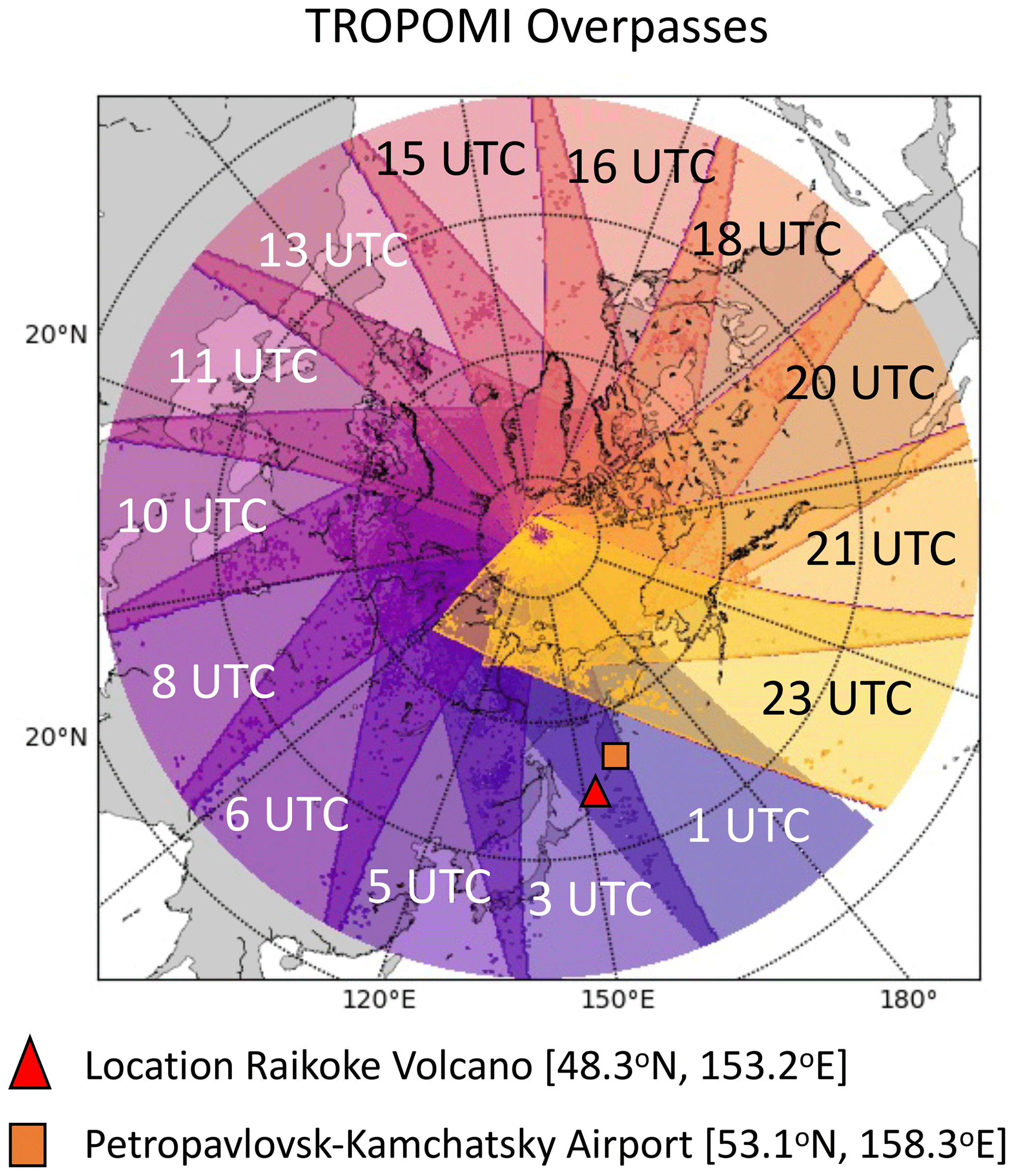
Figure 1Example of daily TROPOMI overpasses (north of 25∘ N, with a swath width of 2600 km). Time indicates the approximate central time for each overpass (each track takes approximately 1.5–2 h). Note the overlap of the swaths, resulting in a higher temporal resolution near the pole. Also shown is the location of the Raikoke volcano (triangle) and the radiosonde location at the Petropavlovsk-Kamchatsky Airport (square).
The International Airways Volcano Watch (IAVW) is responsible for the dissemination of information on the occurrence of volcanic eruptions and associated volcanic ash clouds (ICAO, 2019a) through nine Volcanic Ash Advisory Centres (VAACs). During a volcanic eruption the responsible VAAC disseminates relevant information to the aviation sector regarding the geographic location of volcanic ash present in the atmosphere. Currently, the VAACs are only required to provide forecasts of volcanic ash dispersion, and therefore less development has been achieved on the forecasting of volcanic gas clouds. There is, however, increasing consensus among the scientific community that monitoring and simulating SO2 clouds could be of interest to stakeholders, as volcanic SO2 can pose a public health hazard and potentially affect the aviation industry (e.g. increase of aircraft maintenance costs) (Witham et al., 2012; Schmidt et al., 2014; Carboni et al., 2016; Granieri et al., 2017; Grégoire et al., 2018). Volcanic SO2 clouds are also frequently (but not always) co-located with ash clouds. Detecting ash clouds from satellites retrievals remains a challenging task, and in some circumstances SO2 clouds may act as proxies for ash clouds (e.g. Carn et al., 2009; Thomas and Prata, 2011; Sears et al., 2013; Kristiansen et al., 2015). As a result, the latest roadmap published by the IAVW (ICAO, 2019b) includes SO2 forecasts as a core item to be implemented in the future.
The main tools used by VAACs to provide accurate forecasts of volcanic cloud characteristics are atmospheric dispersion models (ADMs), which are numerical models that simulate how air parcels disperse within the atmosphere. ADMs are used for a large variety of advection-related research, including dust transport, nuclear accidents, forest fires, air pollution, plant diseases and volcanic clouds (Carpenter et al., 2010; Webster et al., 2011; Katata et al., 2015; Schmidt et al., 2014, 2015; Ashfold et al., 2017; Meyer et al., 2017; Osborne et al., 2019). Because of the ash-focused task of VAACs, there has been a strong research focus on improving the simulation of volcanic ash in ADMs and measuring volcanic ash using in situ and satellite measurement techniques (e.g. Witham et al., 2007; Corradini et al., 2011; Prata and Prata, 2012; Mulena et al., 2016; Harvey et al., 2018; Webster et al., 2020). The skill of ADMs in simulating the evolution of SO2 clouds has also been investigated (e.g. Eckhardt et al., 2008; Heard et al., 2012; Boichu et al., 2013; Schmidt et al., 2015) but to a much lesser extent as this has generally been the realm of global climate models interested in the climatic impacts of the periodic stratospheric injections from volcanoes (e.g. Haywood et al., 2010; Solomon et al., 2011; Schmidt et al., 2018).
Observations are vital in determining the skill of the dispersion models. While in situ observations are available for several well-studied volcanoes (e.g. Pfeffer et al., 2018; Sahyoun et al., 2019; Whitty et al., 2020), they are only available for a limited number of locations. In recent decades, many high-resolution remote-sensing measurements have become available, providing a great data source on activity at even the most remote volcanoes across the globe. A large number of satellites now measure atmospheric SO2, with each newly launched instrument having an increased accuracy (see for example Fig. 2 in Theys et al., 2019). The TROPOspheric Monitoring Instrument (TROPOMI) has been operational since the end of 2017 and retrieves atmospheric SO2 total column densities at an unprecedented spatial resolution for UV measurements (up to 3.5 km × 5.5 km at nadir) (Theys et al., 2017, 2019). TROPOMI therefore provides a useful source of information to evaluate model simulations of SO2 clouds using ADMs (and climate models).
One major issue for the development of ADMs for volcanic clouds is the relatively small number of large-magnitude eruptions available since the start of the satellite era in 1979 in order to validate model output. While small-magnitude eruptions take place more frequently, large-magnitude eruptions that can emit large amounts of SO2 into the stratosphere are much more sporadic (e.g. Pyle, 1995; Miles et al., 2004; Carn et al., 2016; Schmidt et al., 2018). The 2019 Raikoke eruption is the first eruption with SO2 emissions in excess of 1 Tg of SO2 that has been observed by the TROPOMI instrument. Due to the amount of SO2 emitted into the stratosphere, it provides an ideal test case to validate the skill of the Numerical Atmospheric-dispersion Modelling Environment (NAME) (Jones et al., 2007), which is the dispersion model used by the London VAAC (Witham et al., 2020). In this paper we will focus on the evolution of the volcanic SO2 cloud during the first 3 weeks after the 2019 Raikoke eruption and compare the output from NAME with the TROPOMI and the Infrared Atmospheric Sounding Interferometer (IASI) satellite SO2 products. In the accompanying Part 2 paper (Osborne et al., 2021), a detailed assessment of the sulfate aerosol together with volcanic ash from this eruption is discussed as well as the effects from biomass burning aerosols that were emitted into the stratosphere from an unusually strong pyrocumulus event in continental North America.
The paper is structured as follows: after discussing the TROPOMI and the IASI satellite SO2 products in Sect. 2.1 and 2.2, we briefly introduce all the relevant aspects of the NAME dispersion model in Sect. 2.3, including the eruption source parameters. Using the introduced input parameters for our 25 d long NAME simulations, we obtain a good qualitative comparison of the simulated SO2 cloud with the TROPOMI satellite SO2 products during the first 3 weeks after the eruption, which we present in Sect. 3.1. A more detailed analysis of the model skill is presented in Sect. 3.2 and 3.3, where we show that the fractional skill score (FSS) and the structure, amplitude and location (SAL) metric (both metrics are introduced in Sect. 2.4) are powerful tools for assessing the skill of the model simulations in comparison to satellite measurements. The NAME simulation skill in terms of the NH-mean SO2 mass burden throughout the first 25 d after the Raikoke eruption is presented in Sect. 3.4, showing a large dependence of the mass burden evolution on the vertical emission profile. We finish with a discussion of our work (Sect. 4) and present the main conclusions in Sect. 5.
2.1 TROPOspheric monitoring instrument
TROPOMI is part of the ESA's S5P satellite launched on 13 October 2017 (Veefkind et al., 2012) and is a polar-orbiting, sun-synchronous, hyperspectral spectrometer that measures Earth-reflected radiances in the ultraviolet (UV), visible, near-infrared and shortwave infrared parts of the spectrum. Atmospheric SO2 vertical column density (VCD, expressed in Dobson units with 1 DU = 2.69×10¹⁶ molec cm−2) is retrieved by applying differential optical absorption spectroscopy (DOAS) (Platt and Stutz, 2008) to the measured ultraviolet spectra in three wavelength ranges (312–326, 325–335 and 360–390 nm). For a more detailed description of the SO2 retrieval, we refer the reader to Theys et al. (2017, 2018).
In our study we use the TROPOMI satellite retrievals across the NH (north of 25∘ N) that cover the Raikoke SO2 cloud between 22 June and 15 July 2019. Figure 1 shows an example of the TROPOMI daily overpasses over the NH. Compared to its predecessors OMI and SCIAMACHY, TROPOMI has a higher horizontal pixel resolution (up to 3.5 km × 5.5 km), allowing for a more detailed characterisation of the small-scale features in volcanic SO2 clouds (Theys et al., 2019). The retrieved TROPOMI SO2 VCD product is calculated by accounting for a large number of parameters, such as meteorological cloud fraction, surface albedo and the vertical distribution of absorbing trace gases (e.g. ozone) (Theys et al., 2017, 2018). As a result, the SO2 retrievals from TROPOMI are sensitive to many assumptions, which can lead to uncertainties of up to ±50 %. For SO2 in the stratosphere, the sum of the various uncertainties can be approximated to be around ±30 % of the retrieved SO2 VCDs. For a detailed discussion of the retrieval uncertainties, see Theys et al. (2017).
One of the largest uncertainties of the TROPOMI SO2 VCD product is the height of the SO2 cloud. However, the sensitivity of the measurement with height is well characterised. To account for this sensitivity, the TROPOMI SO2 VCD level 2 products are publicly available from the ESA website (https://s5phub.copernicus.eu, last access: 22 March 2021) for three different scenarios where the SO2 layer is assumed to be at either 1, 7 or 15 km a.s.l. (above sea level). The TROPOMI VCD data presented in this study are for an SO2 layer at 15 km a.s.l., as this is the height nearest to the estimated weight-averaged emission height for the Raikoke eruption (see e.g. Fig. 2).
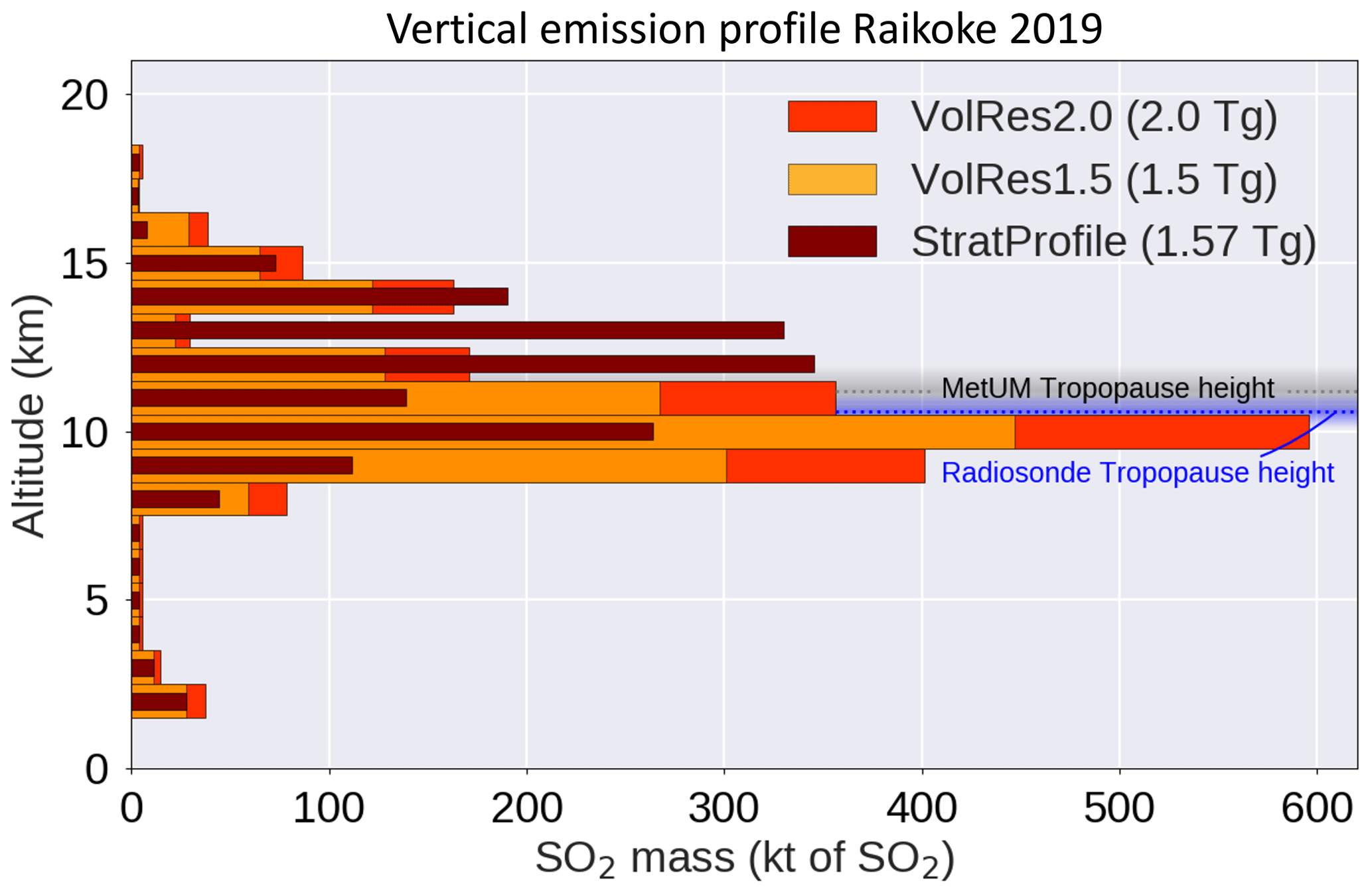
Figure 2Estimated total emitted SO2 mass for the Raikoke eruption between 21 June 2019 18:00 UTC and 22 June 2019 03:00 UTC. The initial emission profile was provided by the VolRes (Volcano Response) team, which is implemented in NAME for the 1.5 Tg SO2 simulation (VolRes1.5, orange). We also simulated the same profile for a 2.0 Tg SO2 emission (VolRes2.0, red). Also included is a new emission profile estimate (StratProfile, brown) based on the TROPOMI SO2 VCD cloud on 23 June (see Sect. 2.3.4). This profile has a similar total mass emitted to VolRes1.5, but a larger fraction (69% instead of 43%) of its mass is emitted in the stratosphere (see Table 2). The grey line represents the average tropopause height in the MetUM during the first 36 h after the eruption at the location of the Raikoke volcano. The blue line and shading represents the average and the range of measured tropopause heights by the radiosondes released from the Petropavlovsk-Kamchatsky Airport (square in Fig. 1) during the first 36 h after the eruption.
In order to compare the available satellite retrievals with any atmospheric dispersion model output, one needs to apply the column averaging kernel (AK) operators to the model data, thereby matching the model-simulated SO2 VCDs to the TROPOMI products. The pre-calculated AKs for the 15 km scenario (Theys et al., 2018) have been applied to the NAME model output. We have repeated the analysis using the AKs and TROPOMI VCDs assuming the SO2 layer at 7 km a.s.l., which affects the absolute SO2 VCDs (not shown) but not our interpretation of the results or our overall conclusions.
To obtain a daily SO2 mass estimate from the TROPOMI measurements, we grid the satellite data and combine all the overpasses during a 24 h period starting at 12:00 UTC of any given day. In the case of multiple overpasses over a single location, we average the SO2 cloud at these grid locations to avoid double counting. For the mass estimate from TROPOMI we have used a detection threshold of 0.3 DU (Theys et al., 2020). The resulting SO2 VCD (in DU) is then converted into a mass (Tg) by using the area of each individual grid point and the molar mass of SO2. Due to the high spatial resolution of the TROPOMI retrieval (on average 9 TROPOMI pixels per output grid cell for the resolution used in the dispersion model), we have downscaled the final TROPOMI retrievals to the output grid resolution of the NAME dispersion model by averaging the SO2 VCDs of all pixels within each NAME grid cell (0.2∘ latitude × 0.4∘ longitude). Unless otherwise specified, we refer to the sulfur dioxide mass burden as the total SO2 mass within the NH, north of 25∘ N.
During the initial stage of the eruption, it is likely that TROPOMI underestimates the SO2 VCDs due to the presence of volcanic ash (e.g. Yang et al., 2010). To understand if ash interference is likely to have affected our SO2 estimates, we also retrieve the absorbing aerosol index (AAI) from the TROPOMI instrument (Zweers, 2016). Although the TROPOMI AAI product should be used with care due to its sensitivity to for example cloud height and optical thickness (see e.g. de Graaf et al., 2016; Kooreman et al., 2020), high index values (>1) indicate the presence of aerosol plumes from dust outbreaks, volcanic ash and biomass burning. During the first 48 h after the eruption we found high peak AAI values within the volcanic cloud (>18.9 on the 22 June and >3.5 on the 23 June), indicating that volcanic ash had an impact on the SO2 retrieval during this period.
2.2 The infrared atmospheric sounding interferometer
The second satellite SO2 dataset used in our analysis is acquired using IASI aboard the MetOp-A and MetOp-B satellites. These satellites operate in tandem on a polar orbit with a field of view (FOV) consisting of four circular footprints of 12 km diameter (at nadir) inside a square of 50 km × 50 km and provide a global coverage twice a day. For our analysis we use the SO2 plume height estimates based on the IASI data, which are produced by applying the retrieval algorithm presented in Carboni et al. (2012, 2016). The IASI instrument also retrieves the SO2 VCDs within the volcanic plume but uses a different set of assumptions in the retrieval algorithm compared to TROPOMI (e.g. IASI retrieves the plume height which affects the SO2 VCD; the retrieved IASI plume height can be different from the plume heights assumed in the TROPOMI product, and therefore the SO2 VCDs from the two methods are not equivalent). To compare SO2 VCDs from NAME to the IASI data, one would therefore also need to apply a different scaling (i.e. AK). As the TROPOMI and IASI retrieval assumptions and limitations are satellite-specific (for example, TROPOMI might detect SO2 closer to the surface than IASI due to the presence of water vapour), a comparison between the two SO2 VCD products is not straightforward and is not attempted here. While it would be an interesting exercise to apply our analysis also to the IASI data, we focus on the comparison of NAME with the TROPOMI SO2 estimates, and therefore no further analysis is done for the IASI SO2 VCD retrievals.
2.3 Numerical Atmospheric-dispersion Modelling Environment (NAME)
The Numerical Atmospheric-dispersion Modelling Environment (NAME) is a Lagrangian model developed by the Met Office (Jones et al., 2007) and is the operational dispersion model used by the London VAAC to forecast the dispersion of volcanic clouds within European airspace (e.g. the Icelandic eruptions of Eyjafjallajökull in 2010 and Holuhraun in 2014–2015). For our work we use NAME version 8.1. The model can trace both ash particles and gases through the atmosphere and includes chemistry parameterisations that allow the conversion of SO2 into sulfate aerosols (SO4) within the volcanic cloud (see Sect. 2.3.3). There is no radiative or chemical interaction between the ash particles and the sulfur species in NAME; the ash particles and sulfate aerosols are thus considered to be externally mixed. In this section we focus on the dispersion of SO2 and highlight the important aspects of NAME for this part of the research. More details on the modelling of ash particles within the model are discussed in the accompanying Part 2 paper (Osborne et al., 2021).
2.3.1 Simulating volcanic cloud dispersion using NAME
Simulating the dispersion of a volcanic cloud with NAME relies on the tracing of air parcels through the atmosphere, each containing an ash, SO2 and/or SO4 mass. These air parcels are released from the source location (volcano), where the user has to define the eruption source parameters (see Sect. 2.3.4). NAME is an offline model; therefore, each parcel is advected by an externally obtained wind field (e.g. a high-resolution Numerical Weather Prediction (NWP) model). In our simulations, we use the wind fields from the latest global analysis of the Met Office Unified Model (MetUM), which have a horizontal resolution of around 10 km at mid-latitudes, 59 levels between the surface and 30 km a.s.l. (decreasing vertical resolution with altitude, with approximately 600 m resolution at tropopause height), and a 3-hourly temporal resolution. The path of each trajectory is calculated using the following equation:
where x(t) is the location of the parcel at time t, x(t+Δt) is the new location of the parcel at time t+Δt, u(x(t)) is the 3D-wind vector at location x(t) and u′(x(t)) represents a stochastic perturbation to the parcel trajectory representing turbulence and unresolved sub-grid mesoscale wind variations in the dispersion model. In NAME, u′ consists of two parts representing atmospheric turbulence () and sub-grid mesoscale diffusion (). The turbulence part represents the stochastic motions from the air parcels due to small-scale perturbations. The mesoscale diffusion represents the horizontal mesoscale motions in the atmosphere that are not captured by the resolution of the used NWP model. Each NWP model has a limited spatial and temporal resolution, and as a result part of the mesoscale features (e.g. eddies) are not captured by the NWP wind field provided. Both the turbulence and mesoscale diffusion within the free atmosphere (excluding the planetary boundary layer, which has a more detailed scheme; Webster et al., 2018) are calculated using
where Kx is a 3D-diffusion vector defined separately for both components, using typical values for the standard deviation of the velocity (σ) and typical time length scales (τ). d represents a random number from a top-hat distribution within the range [−1, 1]. The values for σ and τ are dependent on the NWP model used, as they are impacted by the resolution of the model (Harvey et al., 2018; Webster et al., 2018). The values for σ and τ used in this study are obtained from the analysis done by Webster et al. (2018) and are shown in Table 1. Note that for Kmeso the vertical component () is zero.
Table 1The values for the diffusion parameter K used in NAME. Values are NWP dependent and are given here for the Met Office Unified Model global analysis (10 km horizontal resolution, 59 levels) with a 3-hourly temporal resolution. Values for σ2 are given instead of σ to be consistent with the values presented by Webster et al. (2018). Values are given for both the turbulence Kturb and the mesoscale diffusion Kmeso that are used in NAME for the free atmosphere (i.e. excluding the boundary layer).

Accurately describing atmospheric dispersion due to mixing is a complex three-dimensional problem (e.g. Waugh et al., 1997; Haynes and Anglade, 1997; Haynes and Shuckburgh, 2000; Hegglin et al., 2005; Wang et al., 2020). TROPOMI satellite retrievals provide SO2 VCDs, and therefore our information on mixing effects of the SO2 cloud is limited to their horizontal impact. Studies by Balluch and Haynes (1997) and Haynes and Anglade (1997) have shown that the vertical and horizontal components of stratospheric mixing are related, which allowed them to derive an effective horizontal diffusion from observations. Values reported in the literature for horizontal diffusion coefficients in the lower stratosphere vary over an order of magnitude (103–105 m2 s−1) and also depend on the resolution of the NWP data used (e.g. Balluch and Haynes, 1997; Waugh et al., 1997; Harvey et al., 2018; Wang et al., 2020). To investigate the importance of the horizontal mesoscale diffusion parameter, we present two sensitivity simulations with two different SO2 emissions profiles (see Sect. 2.3.4 for discussion of these profiles) and a reduced value for Kmeso (see Table 2). We decided to only change the Kmeso parameter, as the horizontal Kturb components (see Table 1) are at least an order of magnitude smaller than the Kmeso components, and thus changing them would not show any significant impact on our initial results that is not captured by changing Kmeso. The simulations with a reduced value for Kmeso are indicated by the subscript rd throughout this study. Due to the large range of potential realistic Kmeso values, we have stepwise reduced the parameter and found the best results for a 75 % reduction, which is the value presented in this paper and is similar to the values reported by Balluch and Haynes (1997) and Waugh et al. (1997).
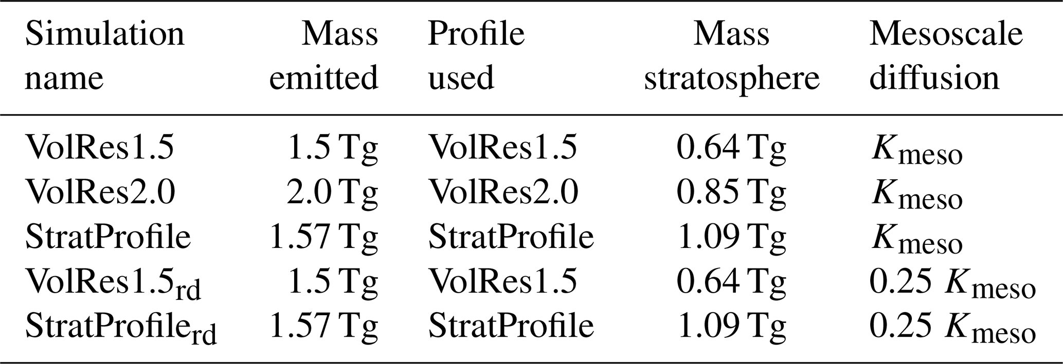
Table 2Overview of the NAME simulations performed using different emission profiles and a reduced mesoscale diffusion (values for Kmeso can be found in Table 1). Also shown is the estimated mass emitted into the stratosphere. For the actual vertical emission profiles, see Fig. 2. All the simulations use the same NWP data input (Global MetUM), the same emission location (48.3∘ N, 153.2∘ E), and duration between 21 June 2019 18:00 UTC–22 June 2019 03:00 UTC. The simulation domain is the NH between 25–90∘ N and the simulation length is 25 d.
2.3.2 Calculating SO2 mass estimates from NAME
In our simulations, the SO2 concentrations (kg m−3) from all the individual air parcels in NAME are presented as hourly means on a regular latitude–longitude grid by calculating the total mass of the SO2 of all parcels in each grid box every hour. The NAME output is calculated using a grid size of 0.2∘ latitude and 0.4∘ longitude (approximately 20 km × 20 km at the latitude of the Raikoke volcano). The vertical resolution of the output is 500 m up to 15 km a.s.l. and 1 km resolution up to 20 km a.s.l., giving a total of 35 levels.
To compare the daily SO2 mass estimates from NAME and TROPOMI, we select the hourly NAME output corresponding to each individual TROPOMI overpass time and select only the grid boxes in NAME that are in the domain scanned by TROPOMI during that overpass. To calculate the SO2 VCD, we apply the corresponding column AK operators obtained from TROPOMI (see Sect. 2.1) to each grid cell of the NAME output. Then for each column on the NAME output grid, the SO2 concentrations (kg m−3) in each grid cell are vertically integrated to obtain the SO2 VCD estimate from NAME.
In all our NAME simulations we found that the SO2 cloud is more diffuse than observed by TROPOMI. Therefore, removing all SO2 VCDs < 0.3 DU in NAME (which is the detection threshold we have used for TROPOMI; see Sect. 2.1) from the simulations would result in a negative bias within the NAME simulation mass estimates that are not related to the evolution of the cloud but due to the stronger diffusion within the model. Therefore we have not included a detection threshold when determining the SO2 mass estimates for the NAME simulations. Similarly to the TROPOMI estimate, the daily mass estimates from NAME are calculated during a 24 h period starting at 12:00 UTC on any given day. The SO2 mass burden is defined as the total SO2 mass (Tg) within the NH, north of 25∘ N.
2.3.3 Chemistry within NAME
NAME contains an atmospheric chemistry scheme (Redington et al., 2009). The relevant chemistry for volcanic clouds is related to the conversion of SO2 into sulfate (). NAME accounts for the oxidation of SO2 in the gas phase using the following reaction:
where HSO3 is then rapidly oxidised to H2SO4 on formation. When water is present in the atmosphere, the oxidation can happen in the aqueous phase by both H2O2 and O3 through the following reaction:
which is followed by
Reactions (R2)–(R6) dominate in cloudy conditions and only occur in model grid boxes when both the meteorological cloud fraction and liquid water content are non-zero. The concentrations of H2O2 and O3 in the atmosphere are pre-defined in the NAME model by using monthly mean background fields obtained from a historical Unified Model coupled to the United Kingdom Chemistry and Aerosol model (UM-UKCA model) simulation that have been smoothed between months using interpolation.
In NAME the SO2 and sulfate aerosol particles can be removed through dry and wet deposition. For our simulations we found that the dry deposition had limited importance for the 2019 Raikoke eruption as most of the volcanic clouds are at high altitudes. Wet deposition in NAME is calculated using a standard depletion equation:
with C representing the SO2 concentration (kg m−3) and Λ the scavenging coefficient, which is calculated based on the rainfall rate r (in mm h−1) and two scavenging parameters A and B. The parameters A and B vary for different types of precipitation (i.e. large-scale/convective and rain/snow) and for different wet deposition processes (i.e. rainout, washout and the seeder–feeder process). For more detailed information, including the specific values for A and B for SO2 and sulfate aerosols, we refer to Webster and Thomson (2014), Leadbetter et al. (2015) and references therein.
2.3.4 Eruption source parameters
When simulating a volcanic eruption, the NAME dispersion model needs eruption source parameters (ESPs) consisting of (1) location, (2) timing, (3) mass eruption rate (kg s−1) and (4) vertical emission profile, and for simulating volcanic ash also (5) particle density, shape and particle size distribution. Here we will discuss ESP 1–4. For information about the set-up of the simulations including ash, we refer to the Part 2 paper (Osborne et al., 2021). For all simulations described in this paper, we released a total of 10 million air parcels in NAME within a column above the volcano, with each parcel representing an equal amount of SO2 mass. All simulations are run for 25 d until 15 July 2019, and the simulation domain is the NH (north of 25∘ N).
In all our simulations (see Table 2 for overview), we release the SO2 from the location of the volcano (48.3∘ N, 153.2∘ E) between 21 June 18:00 UTC and 22 June 03:00 UTC. The timing of the SO2 release is in line with the source term provided by the Volcano Response (VolRes) team (https://wiki.earthdata.nasa.gov/display/volres, last access: 6 July 2021). The VolRes team is an international research collaboration to coordinate a response plan after large volcanic eruptions using observational and modelling tools. No information on the temporal variation in the mass eruption rate was provided by VolRes; thus we assume a constant mass eruption rate throughout the entire eruption period.
The Raikoke eruption injected most SO2 mass near the tropopause height (see Fig. 2), but the precise emission profile is uncertain (e.g. Hedelt et al., 2019; Kloss et al., 2021). Small changes in the SO2 emission profile could lead to a large change in the amount of mass emitted into the stratosphere, which will strongly influence the evolution of the SO2 cloud. Therefore, in our study we use three different SO2 emission profiles that vary in terms of the SO2 mass that is emitted into the stratosphere as shown in Fig. 2. The VolRes1.5 SO2 emission profile is based on the vertical mass distribution obtained from the VolRes team using IASI retrievals on 22 June, as shown by the orange bars in Fig. 2. The total SO2 mass emitted based on the VolRes estimate, which is also the mass emission used in the VolRes1.5 profile, was approximately 1.5±0.2 Tg of SO2.
To determine what fraction of the total SO2 mass was emitted into the stratosphere, we calculated the tropopause height in the MetUM global analysis using the World Meteorological Organization (WMO) temperature lapse rate definition. Using the spread in the 150 nearest grid points to the volcano location in the model, we get an average tropopause height of 11.2±0.7 km during the first 36 h after the eruption. To verify this tropopause height, we used radiosonde data from the Petropavlovsk-Kamchatsky Airport (see Fig. 1), which is the nearest radiosonde location to the Raikoke volcano (data can be retrieved from http://weather.uwyo.edu/upperair/sounding.html, last access: 6 July 2021). Using the same tropopause height criteria for the radiosondes released from this location, we estimate an average tropopause altitude of 10.5±0.7 km during the first 36 h, showing that the MetUM simulated the tropopause height within the expected range. Using the MetUM tropopause height estimate, the VolRes1.5 profile emits 0.86 Tg into the upper troposphere (UT) with a peak at 10 km altitude and emits 0.64 Tg into the lower stratosphere (LS, defined as the layer between the tropopause and 18 km a.s.l.) with a secondary peak at 14 km a.s.l.
In the case of a multi-phase plume like Raikoke (multi-phase here refers to the mixture of ash, sulfate aerosols and gas present in the cloud, not the number of eruption phases), high ash concentrations within the volcanic cloud can interfere with satellite SO2 retrievals (Yang et al., 2010; Carboni et al., 2016; Theys et al., 2017), leading to an underestimation of the SO2 VCDs. Furthermore it is known that, in the stratosphere, ash and sulfate aerosols can have a local heating effect due to their interactions with radiation, resulting in lofting of the SO2, sulfate aerosols and ash (e.g. Niemeier et al., 2009; Jones et al., 2016; Muser et al., 2020; Bruckert et al., 2021). NAME does not account for radiative lofting of volcanic species due to changes in heating rates as it is an offline model driven by NWP wind fields that are not affected by any volcanic ash or aerosols radiative effects.
The fact that Raikoke was an eruption that produced a multi-phase plume that emitted 1.5 Tg of SO2 and 15 Tg of ash (Osborne et al., 2021) near the tropopause (see Fig. 2) justifies simulations using different initial SO2 emission profiles and warrants a closer investigation of the emission profile provided by the VolRes team. To understand potential uncertainties on the VolRes emission profile, we have run an initial 36 h NAME simulation with the VolRes1.5 vertical emission profile input and compared the SO2 VCD estimates (Fig. 3a) with the TROPOMI retrieval on 23 June (Fig. 3b). The comparison reveals that the VolRes1.5 simulation has a different longitudinal distribution compared to the TROPOMI satellite retrievals. Figure 3d shows the averaged SO2 VCDs between 48–52∘ N along section I–II (black box in Fig. 3a) for the clouds shown in Fig. 3a–c. This shows that along the northern part of the cloud between 170–175∘ E, the VolRes1.5 simulation underestimates the SO2 VCDs from TROPOMI by up to a factor of 8.

Figure 3The SO2 VCD estimates for 23 June 2019 for (a) the VolRes1.5 simulation, (b) the TROPOMI retrievals and (c) the StratProfile simulation. The TROPOMI retrievals are downscaled to the NAME simulation resolution, (i.e. averaged per grid box; see Sect. 2.1). The black contours show the pressure at the 10 km a.s.l. in the MetUM analysis used for both NAME simulations. Panel (d) shows the latitudinal SO2 VCDs from panels (a)–(c) along section I–II in panel (a), averaged over the black box between 48 and 52∘ N. Shading represents the standard error estimate for the TROPOMI estimate.
Figure 4 shows the vertical cross section from the VolRes1.5 simulation through the SO2 cloud along section I–II in Fig. 3a, together with the available estimated cloud heights from IASI for all pixels between 49–50∘ N. The cloud height from the IASI retrieval is estimated using the method described in Carboni et al. (2016). Figure 4 shows that the SO2 cloud between 170–175∘ E is simulated in NAME between 11–14 km, which coincides with the UT/LS in the MetUM Global model (see Fig. 2). The altitude of the SO2 cloud for the NAME VolRes1.5 simulation along the cross section shown in Fig. 4 is within the uncertainty range of the IASI height estimates and gives us confidence that the NAME simulated cloud height range is realistic. However, the underestimated SO2 VCDs in the latitude range 170–175∘ E for the VolRes1.5 simulation compared to TROPOMI (Fig. 3) could indicate an underestimation of the mass fraction of SO2 present in the stratosphere, which could be due to the lack of radiative lofting of the SO2 during the first 36 h after the eruption. The study by Muser et al. (2020) shows that after the Raikoke eruption, most of the radiative lofting of the ash layers occurred over these timescales, and we assume similar timescales to be applicable for the lofting of the SO2 clouds. Reducing the horizontal diffusion Kmeso in the VolRes1.5rd simulation (not shown) resulted in a similar underestimate as shown in Fig. 3d for VolRes1.5, excluding that overdispersion in the stratosphere is the main source for the underestimate.
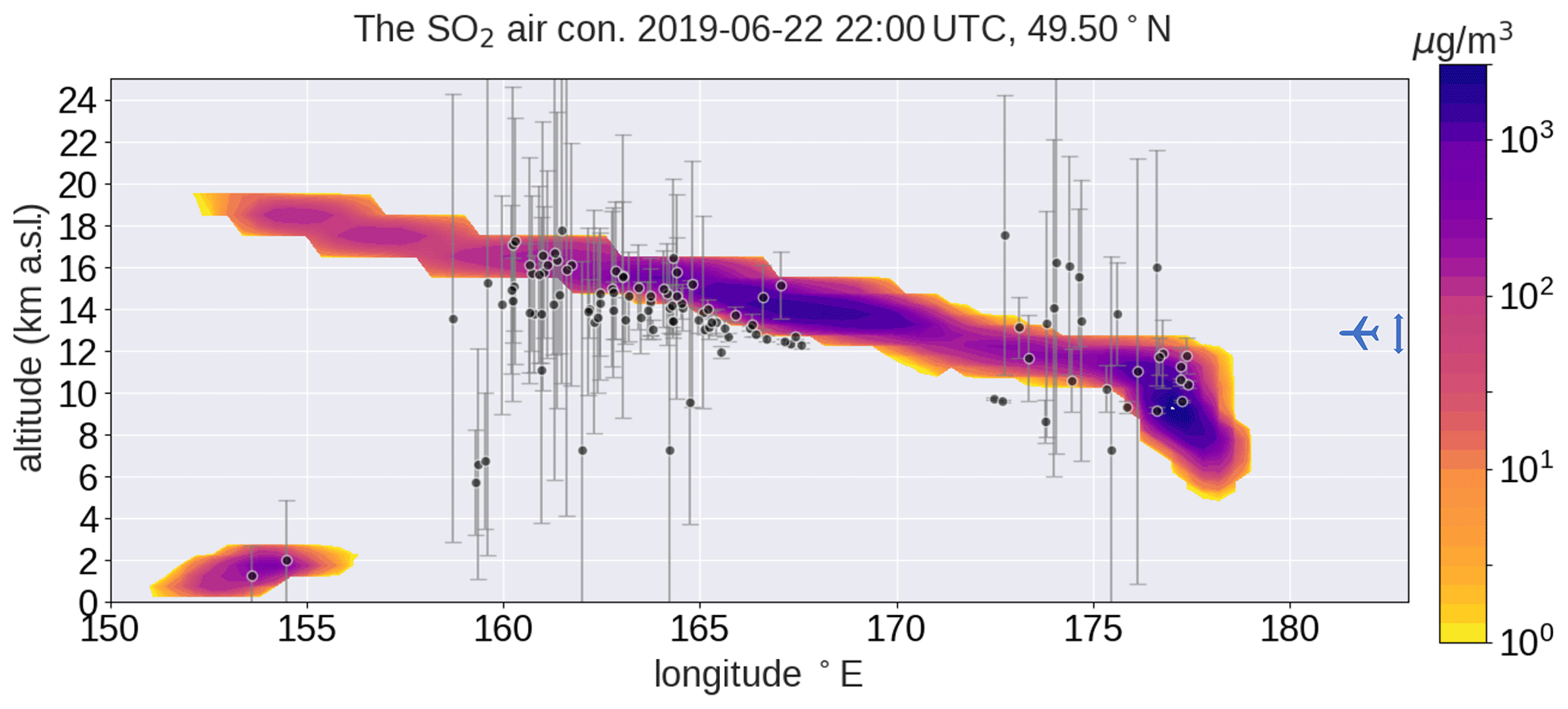
Figure 4Vertical cross section of SO2 mass concentrations (µg m−3) in the VolRes1.5 simulation and the IASI height estimate along the line I–II in Fig. 3a on 22 June 2019 at 22:00 UTC. This time corresponds with the IASI overpass over the volcanic cloud, thereby minimising displacement errors due to timing. The black dots represent the available height estimates including error bars from the IASI retrieval of the SO2 cloud for all pixels between 49–50∘ N, and it is estimated following the method described in Carboni et al. (2016). The blue arrow on the right of the figure indicates the range of cruise altitudes for long-haul aircraft (11.9–13.7 km).
Based on the initial findings from the VolRes1.5 simulation, we also conduct a simulation in which we released a total of 2 Tg of SO2, using the same relative mass distribution in the vertical, termed VolRes2.0. The experiment emits a larger amount of SO2 into the LS (1.15 Tg in the UT and 0.85 Tg in the LS). In chemistry transport models (including NAME), the chemical conversion and the rate of wet and dry deposition of SO2 depends on the SO2 concentration. Therefore this simulation is not a simple scaling of the VolRes1.5 results.
In addition, we derive a different vertical profile based on the TROPOMI SO2 VCD retrievals (StratProfile; for derivation see Appendix A) in which we use a different relative mass distribution in the vertical. In contrast to the VolRes1.5 profile (which is based on the IASI satellite overpasses on 22 June), our StratProfile emission profile is based on the 23 June overpasses of TROPOMI. These overpasses are approximately 30 h after the onset of the eruption and show a reduced ash interference (as seen by the strongly reduced AAI values; see Sect. 2.1); thus we expect the SO2 retrievals to be more accurate. Furthermore, this effective emission profile (Rix et al., 2009; Klüser et al., 2013) will take into account any lofting of the SO2 clouds resulting from the radiation interactions which may be enhanced by the presence of ash during the first 30 h after the eruption. The derived StratProfile emission profile releases similar amounts of SO2 into the atmosphere as the VolRes1.5 run (1.57 Tg) but has the main peak in SO2 mass at 12–13 km altitude. As a result, the StratProfile emits a much higher fraction (69 % or 1.09 Tg) of the mass into the LS (VolRes emission profile emits 43 % or 0.64 Tg into the LS).
2.4 Metrics to determine the skill of the NAME simulations
Assessing the model's skill in representing satellite measurements of SO2 requires appropriate metrics. Similar comparisons should be possible in almost near-real time for VAACs when investigating future eruptions. Therefore, apart from being able to show the details of the model–satellite comparison, it is also important that the metric is easily interpretable by end users. In the following subsections we introduce two metrics for identifying the skill of the simulations: (1) the FSS and (2) the SAL score.
2.4.1 Fractional skill score (FSS)
The FSS was originally developed to determine the skill of weather forecast models to represent radar rainfall observations (Roberts, 2008; Roberts and Lean, 2008; Mittermaier et al., 2013) but has been since used to also describe the skill of dispersion models in representing volcanic clouds (Dacre et al., 2016; Harvey and Dacre, 2016). For volcanic SO2 clouds, the FSS is calculated using the ratio between the model-simulated (Mk) and observed (Ok) fractional coverage of the SO2 cloud at each location (neighbourhood) in the domain investigated. When considering N neighbourhoods, the FSS is calculated using
The FSS is calculated from the fractions Brier score (FBS), which is a variation on the Brier score (Brier, 1950), and FBSref is the largest FBS score one can obtain from multiple non-zero fractions within the domain when there is no overlap between the two fields. In the case that observations and simulation are perfectly aligned, FSS is equal to one. In the case of a total mismatch FSS is equal to zero. In general for the FSS, a model simulation is considered to have skill when FSS > 0.5 (see e.g. Harvey and Dacre, 2016).
The FSS metric is very suitable for studying the skill of a model in capturing the volcanic cloud's spatial extent. One advantage of using the FSS metric is that it relaxes the requirement for exact matching of the spatial features in the simulations with the observations. Instead when the fractional coverage of the SO2 cloud within a studied region (i.e. a neighbourhood of size N) is the same for the observations and the simulation, this metric counts it as a correct forecast. By using different sizes of neighbourhoods, one can also determine at which spatial resolution the simulation is skilful (i.e. for which N is FSS > 0.5) at any given time, which helps to determine at which spatial scale features of the SO2 cloud can be considered realistic. However the method does not consider differences in SO2 VCDs values – it only considers a “hit” or “miss” for each location. By applying the same FSS metric to increasing SO2 VCD thresholds (i.e. subregions of the cloud), one can obtain information about model skill at simulating volcanic SO2 cloud structures with varying vertical column densities.
2.4.2 Structure, amplitude and location score (SAL score)
The SAL score is a metric that is composed of three components, which describe the structure (S), amplitude (A) and location (L) of an investigated feature within a specified domain. The metric was originally developed to compare the structure of model-simulated precipitation fields with observations (Wernli et al., 2008) but has since been adapted to also describe other fields, including volcanic clouds (e.g. Dacre, 2011; Wilkins et al., 2016; Radanovics et al., 2018). Here we will adopt this metric to describe the evolution of the SO2 cloud. For a detailed description of the equations used to calculate each individual component, we refer the reader to Wilkins et al. (2016).
Briefly, to calculate the S and L scores (not needed for the A score), we have to identify all the individual simulated and observed SO2 clouds. In our analysis each cloud is identified as a group of adjacent grid cells which have a SO2 VCD value above a certain threshold. From Theys et al. (2019) we deduce that the detection limit of the satellite measurements for individual pixels is approximately 1 DU. All of the analysis in our study is done at the highest resolution that is available for all fields, which is the NAME model output (0.2∘ latitude and 0.4∘ longitude). Due to the higher spatial resolution of the satellite product, we have to average the TROPOMI output of multiple pixels within each NAME grid box (on average 9 TROPOMI pixels per NAME output grid box at each given time step) to get both datasets on the same output grid. As a result, we have used a lower detection threshold of 0.3 DU when identifying all grid points that are part of a SO2 cloud for the (re-gridded) TROPOMI retrievals and the NAME simulations. To remove additional spurious data from the TROPOMI satellite product, we also include a minimum size of each identified SO2 cloud to be 100 km2 (approximately the NAME grid box size at 50∘ N) before considering in our analysis. Simulated and observed SO2 VCD values below either of these thresholds are excluded from all S, A and L calculations. SAL scores have been calculated by comparing the SO2 VCD estimates from each NAME simulation with the individual TROPOMI overpasses, as well as the daily averages. When calculating the individual overpass SAL score values, we only included the NAME simulation data within the region covered by the TROPOMI overpass.
To interpret the SAL score, we first assume a single idealised 2D-Gaussian-shaped cloud for both the simulated and observed SO2 VCDs. Looking at the schematic cross section presented in Fig. 5, three characteristics are represented by the S, A and L scores. The S score compares the shapes of each individual SO2 cloud in terms of the horizontal extent (width) and maximum concentrations within the cloud, by comparing the normalised shape of the clouds (i.e. total mass of the simulated and the observed clouds are made equal; see Fig. 5a). A negative S score indicates that the simulated SO2 clouds are too narrow or have peak SO2 VCD values that are too high when compared to the observed cloud (leptokurtic). When the simulated SO2 clouds are too wide spread or have peak SO2 VCD values that are too low, this is indicated by a positive S score (platykurtic).
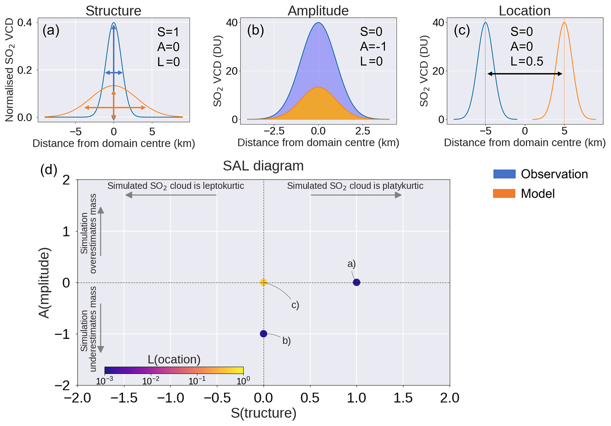
Figure 5Schematic overview of the SAL score and its interpretation, using two cross sections of idealised Gaussian-shaped SO2 clouds. Each panel shows the impact of an individual component of the SAL score: (a) structure, (b) amplitude and (c) location (only the L1 part). A negative S score indicates that the simulated SO2 clouds are too narrow or have peak SO2 VCD values that are too high when compared to the observed cloud (leptokurtic). When the simulated SO2 clouds are too wide spread or have peak SO2 VCD values that are too low, this is indicated by a positive S score (platykurtic). Panel (d) shows an example of the SAL score diagram with the scores of the three cases in panels (a)–(c) included. The horizontal axis represents the S score, the vertical axis represents the A score and the colour of each point represents the L score. When the simulation and observations compare perfectly, the score of each of the components is 0. The simulation and observations compare best when all the points are near the origin and have the dark purple colour.
The A score represents the comparison between the simulated and the observed total mass of SO2 within the entire studied domain and is independent on the number of individual SO2 clouds. Negative A scores represent an underestimate of the total SO2 mass in the simulation when compared to the observations (Fig. 5b), while a positive value shows that the simulation is overestimating the total SO2 mass in the domain.
Finally the L score represents the distribution of the individual simulated and observed SO2 clouds within the domain and consists of two parts: L1 and L2 (Wernli et al., 2008). L1 represents the normalised distance between the domain-averaged centre of mass of all the simulated and observed SO2 clouds, where a higher positive value represents a larger distance between the simulated and observed domain-averaged centres of mass (see Fig. 5c). In the case of multiple SO2 clouds, L2 represents the differences in the distribution of individual clouds around the domain-averaged total centre of mass. L2 is calculated by considering the distance between the centre of mass of each individual cloud and the total domain-averaged centre of mass. In the case of a single object, L2 is equal to 0, as the centre of mass in the domain is the same as the centre of mass of the individual object.
When the simulation and observations compare perfectly, the score of each of the components is 0. For the S and A score the values are all between ±2, where a value of −1 represents a factor of 3 underestimate of the simulation compared to the observations and +1 represents a factor of 3 overestimate of the simulation. For the L1 and L2 scores, values are between [0, 1], with the worst possible score being 1, representing a distance equal to the maximum distance within the domain. Similar to Wernli et al. (2008), we will present the three components of this metric in a SAL diagram (Fig. 5d), where the horizontal axis represents the S score, the vertical axis represents the A score and the colour of each point represents the L score (sum of L1 and L2). The simulation and observations compare best when all the points are near the origin and have the dark purple colour.
First we qualitatively discuss the spatial pattern of the SO2 cloud and its dispersion across the NH during the first week after the eruption. We then discuss the FSS and the SAL scores for the SO2 cloud, followed by a discussion of the SO2 mass burden evolution during the first 25 d after the eruption. A video of the volcanic SO2 and SO4 VCDs as simulated by NAME for the VolRes1.5 and StratProfile emission profiles can be found in the video supplements (de Leeuw, 2020).
3.1 Spatial pattern of the sulfur dioxide cloud
Qualitatively, the general structure of the SO2 cloud simulated by the NAME VolRes1.5 and the StratProfile simulations compare well with the retrieved TROPOMI SO2 VCDs during the first week after the eruption. On 23 June 2019 the TROPOMI retrievals show a split between the northern and southern branch of the SO2 cloud, as seen in Fig. 3. This observed SO2 cloud structure was strongly influenced by a low-pressure cyclone approximately 1500 km to the east of the volcano. As a result of the low-pressure system, the volcanic cloud within the troposphere (below 11 km) moved predominantly in a south-eastward direction along the south flank of the cyclone until it started to wrap around the centre on 23 June. For the cloud layers at higher altitudes within the stratosphere, the main wind direction was more zonal, resulting in the observed split in Fig. 3. The VolRes1.5 and the StratProfile simulations show the same spatial pattern but have different SO2 VCDs within the cloud (see e.g. Fig. 3d). The StratProfile (Fig. 3c) simulation shows a better agreement with the TROPOMI SO2 VCD values for this day, which is expected based on its derivation.
By 25 June 2019, a large part of the cloud moves in a north-western direction, spreading over the Asian continent as seen in Fig. 6a and b for both the VolRes1.5 simulation and TROPOMI. Due to the variation in emission heights between the VolRes1.5 and the StratProfile simulations (Fig. 2), we can identify the parts of the cloud in the NAME simulations that are mainly within the troposphere and the stratosphere by comparing their differences. The results are shown in Fig. 6c, which shows that the north-western part of the cloud is mainly within the troposphere, while the stratospheric parts of the cloud remain centred around the low-pressure system. Calculating the difference between the VolRes1.5 simulation and the TROPOMI retrievals in Fig. 6d, we find that the pattern is very similar to Fig. 6c. This shows that the VolRes1.5 simulation mainly overestimates the SO2 mass of the cloud in the troposphere and underestimates the stratospheric part of the cloud.
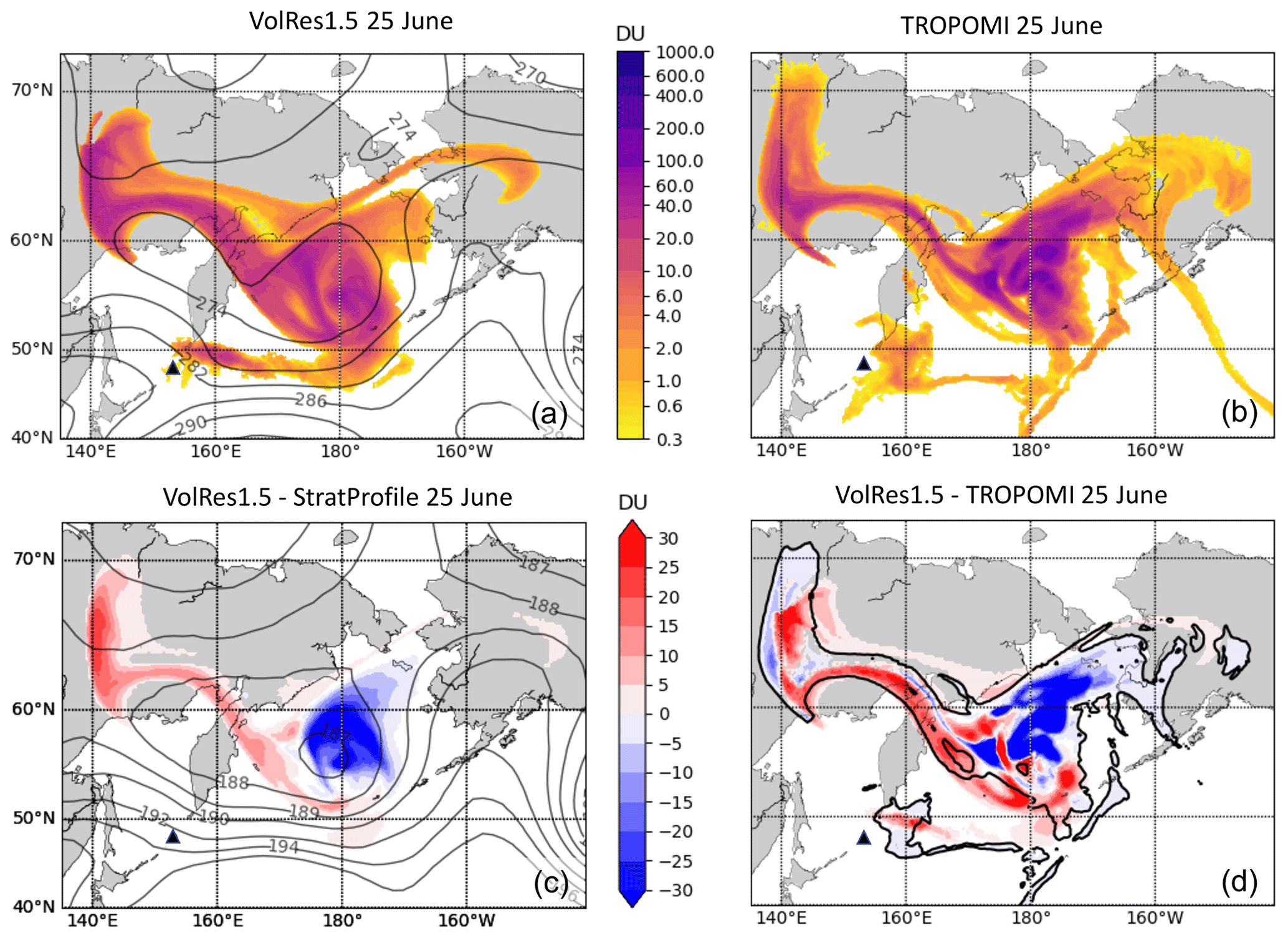
Figure 6The spatial pattern of the volcanic cloud on 25 June 2019. The colours in panels (a) and (b) represent the SO2 VCD for the VolRes1.5 simulation and TROPOMI retrievals respectively. The black contours in panel (a) show the pressure at 10 km a.s.l. Panel (c) shows the difference between the VolRes1.5 and the StratProfile simulations, and the black contours show the pressure at 12 km a.s.l. The negative (blue) values indicate the part of the cloud within the stratosphere, while the positive (red) values highlight the cloud within the UT. Panel (d) shows the difference between panels (a) and (b), where the contour shows the 1 DU contour for the SO2 cloud retrieved by TROPOMI in panel (b).
On 27 June 2019, the SO2 cloud starts to spread also at higher altitudes, leading to a complex spatial pattern as shown in Fig. 7. While the large-scale structure of the cloud on 27 June has become much more complex, both the VolRes1.5 and the StratProfile simulations capture the general SO2 VCD structure of the retrieved TROPOMI cloud well. Note that the small-scale eddies observed by TROPOMI in the centre of the cloud are not simulated by NAME as a result of the limited (spatial and temporal) resolution of the NWP input. Therefore, the small-scale variability cannot be captured by the model but instead is parameterised by the diffusion parameters as a random perturbation on the wind field (see Sect. 2.3.1). This results in the spreading of the SO2 cloud with a smoother pattern in the NAME simulations without the high peak values. This also explains the patchy variations shown in Fig. 6b and c within the centre of the cloud. Averaging the SO2 VCDs over the whole domain shown in Fig. 7 (thereby removing the small-scale features from TROPOMI), the average SO2 VCD values for the VolRes1.5 simulation are 20 % lower than measured by TROPOMI. This is also evident from the dominant blue colours in Fig. 7b. For the StratProfile simulation (Fig. 7c) the domain-average mass is within 0.01 Tg of SO2 of the TROPOMI SO2 mass estimate (i.e. StratProfile SO2 mass estimate is <1 % lower than TROPOMI).
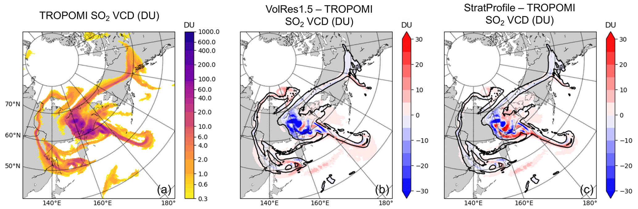
Figure 7The spatial pattern of the volcanic SO2 cloud as retrieved by the TROPOMI satellite for the 27 June 2019 (panel a). Panels (b) and (c) show the difference (in DU) with the VolRes1.5 and the StratProfile simulation respectively. Only SO2 VCD values above 1 DU are shown. The contour shows the outline of the SO2 cloud in TROPOMI for a SO2 VCD of 1 DU.
Finally, we also find a larger spread of the cloud in both the VolRes1.5 and StratProfile simulations as seen in Fig. 7b and c by the red values outside the 1 DU TROPOMI contour. We only included the values > 1 DU in this plot for clarity of the figure. When including lower values (0.3–1 DU), the overestimation of the spread of the cloud in NAME is even larger (not shown here).
3.2 Fractional skill score (FSS)
The VolRes1.5 and the StratProfile simulations are generally able to capture the large-scale structure of the SO2 cloud, but differences between the simulations and the satellite retrievals occur after 4–5 d of simulation (see for example Fig. 6). To determine the timescales for which the simulations show skill compared to the TROPOMI retrievals, we calculate the FSS score for each individual overpass for a range of SO2 VCD contours (ranging between 0.3 and 100 DU). The results for the smallest neighbourhood size N=1 (i.e. the NAME output grid box size 0.2∘ latitude and 0.4∘ longitude) are shown in Fig. 8 for (a) the VolRes1.5 and (b) the StratProfile simulation.
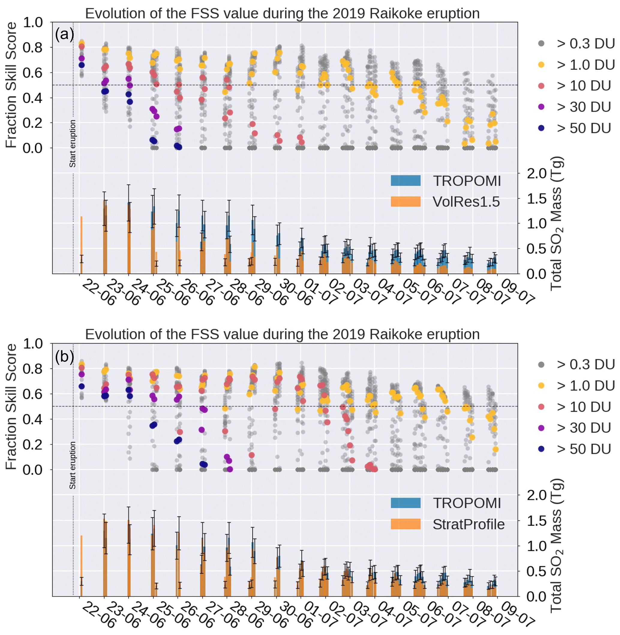
Figure 8Time evolution of the FSS (N=1) and the SO2 mass for each individual overpass of the TROPOMI satellite over the Raikoke cloud for (a) the VolRes1.5 simulation and (b) StratProfile simulation. Each annotated date represents 00:00 UTC. Grey dots represent all concentrations between 0.3 and 100 DU, with the highest skill score for the lowest concentrations. The horizontal dashed line shows a value of FSS = 0.5, which is the cut-off value for determining the skill of the simulations.
The VolRes1.5 simulation is able to capture the overall outline of the cloud well for this period but struggles to simulate the peak SO2 VCD values within the retrieved TROPOMI SO2 cloud. Focussing on the SO2 VCD > 1 DU points in Fig. 8a, the simulation has skill (FSS > 0.5) for up to 12.5 d after the eruption onset. This shows that the simulation captures the overall dispersion of the cloud well, as it is able to distinguish between areas with and without any SO2 across the NH. For SO2 VCDs greater than 30 DU, which correspond to small-scale features within the volcanic cloud, the simulation has no significant skill beyond 2.5 d after the start of the eruption. This agrees with the fact that the VolRes1.5 simulation was not able to capture the peak values on the 25 June 2019 observed by TROPOMI as shown in Fig. 6.
The FSS values for the StratProfile simulation (Fig. 8b) reveal that this simulation performs better than VolRes1.5 and has skill on a longer timescale for all of the SO2 VCDs. For the lower SO2 VCDs (<1 DU), the StratProfile simulation remains skilful 2 d longer than the VolRes1.5 simulation (12.5 d versus 14.5 d). For the SO2 VCDs above 30 DU, the FSS skill timescale has doubled compared to the VolRes1.5 simulation, showing again the importance of the emission profile on the skill of the simulation.
The timescales for which the NAME simulations show skill (compared to the TROPOMI retrievals) in terms of FSS are shown in Fig. 9 and Table A1. Independent of the neighbourhood size, the StratProfile simulation has the highest skill for all SO2 VCDs. Figure 9 shows that the StratProfile simulation is skilful on timescales twice as long for SO2 VCD values above 10 DU compared to the VolRes1.5 and VolRes2.0 simulations. Interestingly the change in neighbourhood size (i.e. averaging region) has only a limited impact on the skill timescales for low SO2 VCDs (below 5 DU). This shows that all of the simulations are able to capture the horizontal extent of the SO2 cloud well on spatial scales similar to our smallest output grid used () and on timescales of 2–3 weeks after the start of the eruption.
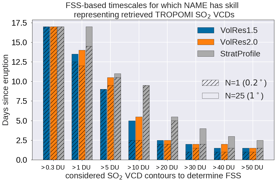
Figure 9The timescales for which the NAME model shows skill based on the FSS, when compared with TROPOMI retrievals. The results are shown for the three simulations as discussed in Sect. 2.3.4 and for two different neighbourhood sizes (value in brackets represent the corresponding resolution). The FSS metric is calculated only for the first 17 d of the simulation (up to 10 July), as the SO2 VCD values become too small after to give a good estimate of the FSS from the TROPOMI measurements.
The reduction in FSS scores for high SO2 VCDs is influenced by two factors. (1) Does the simulation capture high SO2 VCDs. And if so (2) is the location of the high VCD features in the SO2 cloud (see e.g. Fig. 7c) correct? Due to the dispersion of the SO2 cloud with time, we expect a decrease in the FSS values in time for the higher SO2 VCDs as these concentrations are not present anymore in either the TROPOMI retrievals or the NAME simulations (resulting in FSS = 0). The skill timescales are therefore expected to reduce as the SO2 VCDs increase. The StratProfile simulation contains higher SO2 VCDs throughout the simulation period compared to the VolRes1.5 and VolRes2.0 simulations, resulting in higher FSS values and longer relative skill.
For high SO2 VCDs, the FSS metric depends more on the used neighbourhood sizes as the corresponding SO2 cloud features get smaller. Using a larger neighbourhood size compares the presence of small-scale features over a larger region, reducing the impact of any misplacement, and results in a higher FSS. The SO2 VCD values at which model skill increases for different neighbourhood sizes is therefore linked to a displacement error. In Fig. 9, a doubling in skill timescales is found for the larger neighbourhood size (hashed versus non-hashed) at SO2 VCDs > 10 DU for the VolRes1.5 and VolRes2.0 simulations, while for the StratProfile similar differences are evident for SO2 VCDs above 30 DU. This shows that the VolRes1.5 and VolRes2.0 simulations are able to represent observed small-scale features within the SO2 cloud for VCDs up to 10 DU at timescales less than 5 d. For SO2 VCDs > 20 DU these two simulations gain no additional skill with an increased neighbourhood size and show a strong reduction in skill timescales. This indicates that the high SO2 VCDs (>10 DU) observed by TROPOMI are not simulated anywhere in the SO2 cloud at timescales longer than 5 d. For the StratProfile simulation, features with SO2 VCDs above 30 DU are still present up to 4 d. However, these features are slightly displaced, as evident from the increase in the FSS skill timescales from increasing the neighbourhood size from 0.2 to 1∘.
On timescales longer than 5 d, all the NAME simulations show a strong diffusion in the SO2 cloud (related to the diffusion parameterisations). As a result none are capturing the high SO2 VCDs retrieved by TROPOMI, which reduces the FSS for these high values quickly to 0. This shows that high SO2 VCDs within the SO2 cloud are only skilfully simulated on timescales less than 5 d.
3.3 The SAL score
Figure 10 shows the SAL scores for all the individual TROPOMI overpasses and the daily average values for four different NAME simulations. This comparison shows the strength of the SAL diagram to determine what aspects of the SO2 cloud are captured well by the NAME simulations and where the simulations are struggling to match the TROPOMI retrievals. At the start of the eruption, all simulations are in the top half of the diagram (positive A score). This indicates that the simulations have a larger total SO2 mass than the TROPOMI retrievals during the first days after the eruption. This can be partly explained by the presence of ash interfering with the TROPOMI retrievals (see Sect. 3.4). Furthermore the S values are close to 0, indicating that the shape of the cloud is captured well within the simulations. The low L values throughout all the simulation indicate that the location of the SO2 clouds is well captured.
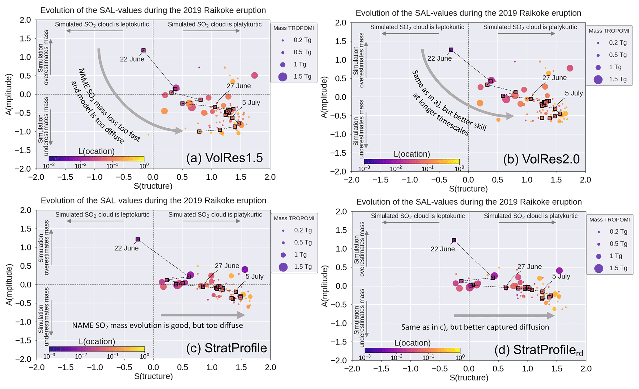
Figure 10Time evolution of the SAL values for four different NAME simulations: (a) VolRes1.5, (b) VolRes2.0, (c) StratProfile and (d) StratProfilerd. The black dashed line shows the daily average evolution of the S and A parameters between 22 June and 10 July, while the coloured squares show the daily average values of L. The coloured dots represent the SAL values for each individual TROPOMI overpass as shown in Fig. 2. To obtain the A parameter, we have excluded the SO2 VCDs of TROPOMI below 0.3 DU to reduce noise but included all mass for the NAME simulations (see Sect. 2.3.2).
All four simulations shown in Fig. 10 show a tendency of increasing positive S score values with time, with a strong increase on 27 June, which is 5 d after the start of the eruption. An increase in the S score represents an SO2 cloud which is more widespread (platykurtic) in the simulations compared to the SO2 VCDs obtained from TROPOMI. The largest changes in the S score around 5 d into the simulation are consistent with our FSS analysis where we identified that this is also the time where the VolRes1.5 and the StratProfile simulations are losing the skill to represent high SO2 VCDs retrieved by TROPOMI (i.e. not capturing the peak values in the cloud).
Focussing on the VolRes1.5 and the VolRes2.0 simulations (Fig. 10a and b), both SAL diagrams show a similar pattern (moving from the top left towards the bottom right in the diagram). Due to the total emitted SO2 mass being greater in the VolRes2.0 simulation, Fig. 10b shows a more positive A score during the first 4 d after the eruption (22–26 June) than the VolRes1.5 simulation as the former overestimates the total SO2 mass retrieved by TROPOMI. After 26 June, the A score for VolRes2.0 remains close to the A=0 line in Fig. 10b, showing that the total SO2 mass compares better with TROPOMI for the VolRes2.0 simulation than the VolRes1.5 simulation after 5 d. For the StratProfile simulation (Fig. 10c), the comparison with TROPOMI is better throughout the entire simulation than for the VolRes1.5 and the VolRes2.0 simulations, as is evident by the low A score as well as the low L score. The comparison between the StratProfile simulation and TROPOMI for each individual TROPOMI overpass (i.e. each dot in Fig. 10c) is close to the A=0 line in the diagram, showing that NAME is able to capture the total SO2 mass very well. Also a lower L score (darker colour of the squares and circles) indicates that the model captures the location of the cloud more accurately than both the VolRes simulations. These results are consistent with the results shown in Figs. 6–9.
Reducing the horizontal diffusion parameter by 75 % (Kmeso; see Table 2) in the StratProfilerd simulation (Fig. 10d) reveals a relative decrease in the S score during the first week (e.g. S=0.5 for StratProfile versus S=0.1 for StratProfilerd on 25 June) and no change in the A and L scores when compared to Fig. 10c. This behaviour is expected, as a decreased diffusion will not alter the total mass (A score) or the centre of mass of the individual SO2 clouds (L score), but it will result in more concentrated SO2 clouds (reduction of S). As a result, the StratProfilerd simulation shows the best comparison with the TROPOMI retrievals for the first 4 d of the eruption (up to 26 June). After that the S score quickly increases for all the simulations independent of the diffusion parameterisation, as diffusion related to uncertainties from the large-scale meteorological conditions (i.e. synoptic-scale uncertainties) starts to dominate the signal.
3.4 Sulfur dioxide mass burden
Figure 11a shows the SO2 mass burden evolution calculated from the TROPOMI satellite retrievals and three NAME simulations (VolRes1.5, VolRes2.0 and the StratProfile) for the 25 d between the start of the eruption and 15 July 2019. The best comparison is obtained using the StratProfile simulation, which captures both the peak value and the long-term evolution remarkably well and falls well within the uncertainty range of the TROPOMI estimate. To obtain the mass burden, we have excluded the SO2 VCDs of TROPOMI below 0.3 DU to reduce noise but included all mass for NAME simulations as discussed in the methods section. It is likely that TROPOMI underestimates the SO2 VCDs and thus SO2 mass during the initial phase of the eruption due to the presence of volcanic ash, which is supported by large values of AAI obtained from TROPOMI during the first 2 d after the eruption (see grey bars Fig. 11a and also Sect. 2.1).
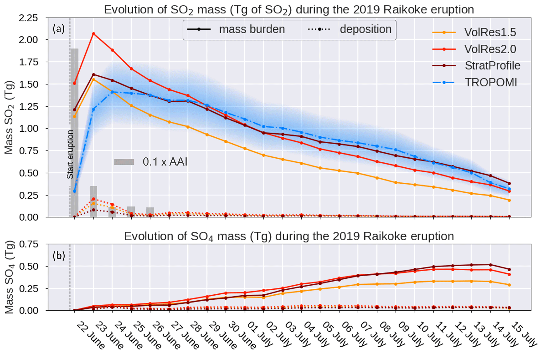
Figure 11The daily evolution of (a) the total SO2 mass (Tg of SO2) and (b) the total SO4 mass (Tg of SO4) for the 2019 Raikoke eruption for different ESPs in NAME. We have included the TROPOMI SO2 mass estimate (blue dashed line) as well as the evolution of three NAME runs: VolRes1.5, VolRes2.0 and StratProfile (see Fig. 2). The dotted lines in the figures show the corresponding daily deposition of SO2 and SO4 from the simulations. The peak values in the NAME SO2 mass distribution are slightly higher than the mentioned total emission values in Table 2, which is the result from applying the 15 km AKs to the dispersion model data. The total SO2 mass burden for TROPOMI is calculated using all locations where the vertical column densities are above 0.3 DU, while for the NAME simulations we include all mass. The blue shading represents the standard error estimate for the TROPOMI product. The grey bars show the TROPOMI estimated 0.1 × max(AAI) value inside the volcanic cloud for the first 5 d after the eruption. The high AAI values during the first 48 h indicate high concentrations of ash, thereby affecting the TROPOMI SO2 retrievals during this period.
Consistent with Figs. 3, 6 and 7, the VolRes1.5 simulation captures the peak in total SO2 mass within the uncertainty of the TROPOMI estimate but underestimates the TROPOMI SO2 mass between 27 June and 15 July 2019 by 0.3 Tg on average. Based on the data shown in Fig. 11, we calculated an e-folding time of ≈9 d for the VolRes1.5 simulation and an e-folding time of ≈21 d for TROPOMI during the first 6 d after the eruption (23–27 June 2019), showing that the VolRes1.5 simulation loses SO2 mass at a much faster rate than that calculated based on TROPOMI. As a result, this leads to an underestimation of 25 % (0.33 Tg) of the VolRes1.5 simulation compared to TROPOMI on 28 June. From 27 June the loss rate for both TROPOMI and VolRes1.5 is similar, with an e-folding time of ≈14–15 d, which is within the range reported in the literature for extratropical summer eruptions of similar magnitude (e.g. e-folding time of 9–18 d for Kasatochi 2008 and 11–14 d for Sarychev 2009) (Karagulian et al., 2010; Krotkov et al., 2010; Haywood et al., 2010; Jégou et al., 2013; Höpfner et al., 2015; Carn et al., 2016).
After 27 June 2019, the total SO2 mass burden evolution from TROPOMI is best captured by the VolRes2.0 and the StratProfile simulations, related to a larger amount of mass emitted into the stratosphere. From the total SO2 mass emitted into the stratosphere calculated in Table 2, we see that both the VolRes2.0 and the StratProfile respectively emit 0.2 and 0.45 Tg more SO2 mass into the stratosphere than the VolRes1.5 simulation. For the VolRes2.0 simulation the overall evolution of the SO2 mass profile is similar to that obtained from the VolRes1.5 simulation (e-folding time of ≈9 d during the first week and e-folding time of 14–15 d afterwards). However, due to the increased total SO2 emissions (0.5 Tg more than VolRes1.5), the SO2 mass evolution of VolRes2.0 also overestimates the TROPOMI peak mass by more than 0.5 Tg on 23 June. Given that TROPOMI is used as our baseline metric for initialising our StratProfile simulations, it is not surprising that the best comparison with TROPOMI during the start of the eruption is obtained for the StratProfile simulations. However, on longer timescales the influence of other factors (e.g. simulated wind field, radiative heating, mixing) on the dispersion of the SO2 cloud means that the model simulation could easily diverge from the observations. That the StratProfile continues to best match the TROPOMI data gives confidence that NAME captures the main processes needed to represent the SO2 dispersion well.
A possible cause for the strong reduction in total SO2 mass during the first week for the VolRes1.5 and VolRes2.0 simulations might be too strong a conversion of SO2 into sulfate aerosols during the start of the simulation. To test this hypothesis, we also calculated the mass evolution of SO4 in NAME, which is shown in Fig. 11b. From this we can conclude that the chemical conversion into SO4 is realistic within the NAME simulations. The daily rate of production of SO4 is small (less than 0.03 Tg d−1), which is a factor of 3 lower than the average daily decrease in SO2 mass in the VolRes1.5 and VolRes2.0 simulations during the first week (0.1 Tg d−1).
The daily total SO2 mass deposition from the NAME simulations is shown by the dotted lines in Fig. 11a. For 23 and 24 June, the total daily wet deposition dominates the removal of SO2 from the atmosphere, as it is responsible for 89 %–90 % of the SO2 mass reduction for the VolRes1.5, the VolRes2.0 and the StratProfile simulations. Atmospheric conditions during the first week of the eruption can explain this relatively large contribution from wet deposition. During the first week of the eruption, the SO2 cloud is moving within a region of moist air in the warm conveyor belt on the southern edge of the cyclone (see Fig. 3). This favours the chemical conversion of SO2 into SO4 through aqueous-phase chemistry and also the removal of SO2 through wet deposition, resulting in the peak deposition values in Fig. 11a. The cyclone is mainly a tropospheric phenomenon, and as a result wet deposition occurs mostly in the tropospheric part of the SO2 cloud. As the VolRes2.0 simulation emits the largest amount of SO2 into the troposphere (see Fig. 2), this also explains the highest removal rate (red dotted line Fig. 11a peaks at 12 % of the NH-mean daily SO2 mass burden on 23 June) and also the highest conversion rate during the first week of the simulation (evident from the largest SO4 mass burden in Fig. 11b in this period). The wet deposition is lowest for the StratProfile simulation during 23 and 24 June (peaks at 4 %–5 % of the NH-mean daily SO2 mass burden on 23 June), as less mass is emitted into the troposphere for this profile.
The results from Fig. 11 show that there is a high sensitivity of the mass burden evolution in NAME to the vertical emission profile used for this particular eruption, which straddled the tropopause. Due to different atmospheric conditions within the troposphere and stratosphere, the SO2 mass burden evolution is different within the two layers, resulting in significant differences in the total SO2 mass burden evolution in our simulations. The average e-folding time of SO2 in the UT is ≈10 d (e.g. Krotkov et al., 2010; Carn et al., 2016), which is consistent with the e-folding time simulated during the first days of the VolRes1.5 and VolRes2.0 simulations. However, the longer e-folding time obtained for TROPOMI for the first 10 d suggests that the bulk of the SO2 mass was not emitted into the UT.
After 10 d a large fraction of the tropospheric SO2 mass is removed from the atmosphere through wet deposition or converted into SO4, and the remaining signal in Fig. 11 is dominated by the stratospheric component of the cloud. This part of the cloud is much less affected by the cyclone, and the stratosphere contains much less moisture. Therefore SO2 is removed at a much lower rate (SO2 deposition is <1 %) and is mainly converted through the gas-phase reaction with OH, resulting in the longer e-folding time of approximately 14–15 d. The similarity in e-folding time obtained from TROPOMI and all the simulations between 27 June and 15 July suggests that the chemistry scheme in NAME is realistic.
Overall, the total SO2 mass burden obtained using the StratProfile emission profiles (both StratProfile and StratProfilerd give the same mass evolution) compares best with TROPOMI. Based on this comparison, we estimate that the 2019 eruption of Raikoke emitted approximately 0.9–1.1 Tg of SO2 into the lower stratosphere (11–18 km a.s.l.). With a maximum SO2 mass burden of 1.5–1.6 Tg in the atmosphere, it follows that approximately 0.4–0.7 Tg was emitted into the UT (8–11 km a.s.l.).
Our study shows that the NAME simulations compare very well with the TROPOMI satellite retrievals of the SO2 cloud during the first 3 weeks after the 2019 Raikoke eruption. Despite the increasing complexity of the SO2 cloud's horizontal structure over time, all our simulations are able to capture the outermost extent of the cloud within an accuracy of approximately 0.4∘(50 km) during the first 2 weeks of the simulations and for up to 25 d with an accuracy of approximately 1∘ (100 km) (see Figs. 8 and 9 and Table A1). While simulated SO2 concentrations within the cloud are strongly dependent on the ESPs, the general dispersion patterns of the SO2 cloud are captured very well in both the troposphere and the stratosphere for all the NAME simulations performed (see Figs. 3, 6 and 7). Combining this information with the comparison of the vertical profile from IASI (Fig. 4) and the included representation of the sulfur chemistry in the NAME simulations (Fig. 11) gives us confidence that the NAME model is able to simulate the 3D structure of the volcanic SO2 cloud (and consequently the SO4 cloud) for the 2019 Raikoke eruption.
While the NAME model was not developed specifically to simulate stratospheric volcanic SO2 clouds, our results show that the model is suitable to be used by VAACs to issue forecasts on the evolution of volcanic SO2 clouds in the upper troposphere/lower stratosphere. Currently after a volcanic eruption, VAACs provide information on the areas in the atmosphere where volcanic ash is forecasted up to 18 h into the future. In the case of the Raikoke 2019 eruption, we have shown that a similar approach to produce a forecast for the presence of a SO2 cloud would have been accurate on this and even longer timescales. However, future SO2 cloud forecasts will more likely be based on designated SO2 concentration thresholds. From our simulations we found that NAME is able to capture the horizontal extent of the 1 DU SO2 VCD contour on a spatial resolution of during the first 17 d after the eruption. Assuming that the obtained SO2 VCD values are from a cloud at 12 km altitude with a thickness of 2 km (e.g. estimated from Fig. 4), 1 DU would correspond to an average SO2 concentration of 0.02 ppm within this cloud. As reference, based on sulfur dioxide acute exposure guideline levels (AEGL) (National Research Council Committee, 2010), an extended exposure (>10 min) to SO2 concentrations of 0.2 ppm (lowest AEGL) can lead to some respiratory irritation, while concentrations above 0.75 ppm can lead to long-lasting adverse health effects. For our example, the lowest AEGL threshold would therefore correspond to SO2 VCDs above 10 DU. We find that NAME is capable of capturing the spatial distribution of the features within the SO2 cloud where the SO2 VCDs are larger than 10 DU on the order of 7–10 d (see Fig. 9).
Our work highlights that accurate information on ESPs is key when comparing model simulations to satellite retrievals. In reality it can be difficult to obtain this information, especially in near-real time. For example, observations show that the Raikoke eruption was actually characterised by a series of explosive eruptions that emitted SO2 at varying heights (Crafford and Venzke, 2019; Hedelt et al., 2019; Muser et al., 2020; Kloss et al., 2021). Furthermore a study by Prata et al. (2021) suggests that activity continued until 10:00 UTC on 22 June rather than 03:00 UTC as reported by the VolRes team. These examples indicate how hard it is to obtain a “correct” time-dependent emission profile for the eruption in near-real time. Instead, the profiles used in this study try to capture the time-averaged emission profiles of these “pulses” during the eruption. To test the importance of the emission duration, we conducted some additional simulations where we increased the duration of the eruption to 10:00 UTC on 22 June. The results of these new simulations (not shown) were very similar to the results presented in this paper, with the main difference that the structure of the cloud is slightly more diffuse.
For all the simulations we find that small changes in the vertical emission profile lead to a large change in the amount of mass emitted into the stratosphere, due to the emissions spanning the tropopause. In our analysis the mass-averaged emission height in the VolRes and StratProfile emission profiles differs by only 1 km (10.5 km in VolRes versus 11.5 km in StratProfile). But in the StratProfile emission profile we emit 69 % (1.09 Tg) of the total SO2 mass above the tropopause (as defined by the MetUM NWP), compared to 43 % (0.64 Tg) in the VolRes1.5 simulation.
NAME does not account for any radiative lofting effect and thus an emission profile derived during the first hours after the eruption could lead to SO2 at the wrong altitudes. Muser et al. (2020) show that for the Raikoke 2019 multi-phase plume, the radiative lofting effect for ash is on the order of 2–3 km during the first days after the eruption. While the precise impact of such a lofting effect on the SO2 cloud is difficult to quantify (Bruckert et al., 2021; owing to lack of knowledge of the details of the relative vertical position on the SO2 and the ash, and the lack of knowledge of the mixing state between the resulting sulfate aerosol and ash), it could help to explain the differences seen between the emission profiles used in this study. For the VolRes1.5 emission profile, which was derived during the first hours after the eruption, the radiative lofting effect is still limited. Instead for the StratProfile, which is derived 30 h after the eruption onset, the radiative lofting has very likely impacted the SO2 cloud vertical structure as Muser et al. (2020) show that most of the lofting took place during the first 36 h after the Raikoke eruption. Therefore, we get a better comparison between the NAME simulations and observations by determining an effective emission profile from 1–2 d after the initial emission time to account for potential radiative lofting effects. Our study results show that the potential impact of radiative lofting should be considered by VAACs when producing forecasts for multi-phase plumes near the tropopause.
Interestingly while the fractional split of the mass between the stratosphere and troposphere is important, the detailed vertical distribution of SO2 within each of these two layers has only a minor effect on model performance. To test the sensitivity of the model results to the details of the vertical distribution of the emissions within the troposphere and stratosphere, we performed a simulation where we emitted 1 Tg evenly between 11–14 km and 0.5 Tg evenly between 9–11 km (not shown). The general conclusions were the same as shown for the StratProfile, illustrating that, for the 2019 Raikoke eruption, it is key to establish the fraction of the SO2 mass that was emitted into the stratosphere.
Also an error in the definition of the tropopause height within the MetUM (or any other NWP) model can have a large influence on the skill of the dispersion simulations. If, for example, the MetUM model-estimated tropopause height is 2 km above the actual observed tropopause height, this would lead to a wrong placement of the majority of the SO2 mass in the troposphere in our VolRes1.5 simulation. Using a different NWP model with a lower tropopause height in the NAME simulations would result in a higher fraction of the SO2 mass of the VolRes1.5 profile being emitted into the stratosphere and potentially give a better comparison with TROPOMI than the StratProfile estimate (which would overestimate the stratospheric SO2 mass in that case). However, we found the average tropopause height of 11.2±0.7 km diagnosed in the model at the eruption site is in good agreement with the observed tropopause height of 10.5±0.7 km from a nearby radiosonde location (see Fig. 2), which gives us confidence that our StratProfile emission estimates for the stratosphere and troposphere are suitable and that the NAME results are not strongly biased by a wrong tropopause height within the NWP fields.
While we have investigated the impact of changing the vertical SO2 emission profile (see Fig. 2), we have not investigated the effect of any uncertainty related to the atmospheric conditions in the NWP wind fields used as input for the NAME simulation. A study by Dacre and Harvey (2018) shows that the impact of the atmospheric conditions on the NAME simulations can be large, especially in conditions of large horizontal flow separation in the atmosphere. The specific atmospheric conditions for this particular eruption (i.e. the low-pressure system east of the eruption site) show isobars that are parallel to each other during the first days after the eruption in the region of the cloud (Fig. 3). Therefore, it is expected that the impact of flow separation is limited during the initial stages of the cloud evolution. After several days, the flow separation becomes more pronounced in various regions in the domain (see Fig. 6). This effect is also reflected in the decrease in the S score value of the SAL diagram shown in Fig. 10, as trajectories start diverging in these regions of enhanced flow separation enhancing dispersion in the model. To better understand the impact of the NWP wind field variability on our results presented here, the analysis would need to be repeated using an ensemble of NWP wind field forecasts as input for the NAME simulations.
Our study of the 2019 Raikoke eruption demonstrates the strength of the SAL diagram for performing a comparison of model simulations with satellite observations and can help to determine potential issues. In this particular case, the NAME model simulations generally tend to show increasing positive S score values for all the simulations. Partly this is related to the diffusion parameterisation in the model, which smooths the signal (i.e. random perturbation) of the small-scale eddies within the cloud that are not present in the input wind field (see Sect. 2.3.1). As uncertainties from the meteorological conditions used as input for the simulations gradually accumulate, this leads to a larger spread in the SO2 cloud over time than is observed in reality. This gives the tendency for the model to be more diffuse on longer timescales, as revealed by the S score increase in Fig. 10a–c.
We find that the key reason for the increasing S score values on shorter timescales (i.e. 1–5 d) is related to the horizontal diffusion parameter Kmeso used for the model simulations. NAME v8.1 uses a single value for the diffusion coefficient within the free atmosphere (see Table 1). From literature it is known that mixing in the atmosphere can be highly variable and seasonally dependent (e.g. Haynes and Shuckburgh, 2000; Allen and Nakamura, 2001; Legras et al., 2005; Abalos et al., 2016). Furthermore, the diffusion parameter values currently used in NAME have been determined using observational datasets near the surface (Webster et al., 2018). It is therefore possible that the mesoscale diffusion values used in the model might be unsuitable for the higher levels in the atmosphere, especially in the stratosphere, and thereby cause too much diffusion from the start of the eruption. To test this hypothesis, we investigated several simulations with a smaller horizontal diffusion coefficient (see Table 2), where we reduce the mesoscale diffusion value Kmeso by 75 % for the whole atmosphere above the boundary layer. The resulting values for the FSS score and SAL diagram for the StratProfilerd simulation are shown in Fig. 10d and Table A1 and indicate that the simulations are better able to capture the structure (i.e. peak values and horizontal extent) of the cloud during the first 5 d of the simulations. It is currently impossible to determine a more precise value for the diffusion parameters, due to the lack of case studies and limited available observations for these high altitudes. Part of ongoing work is to investigate the impact of a new space and time-varying free-atmospheric turbulence scheme that is included in the latest version of NAME (Dacre et al., 2015), which was not available for the simulations presented in this paper.
A previous study by Harvey et al. (2018) used a multi-level emulation approach to better understand the influence of model parameters on the accuracy of NAME output for volcanic ash concentration during the 2010 Eyjafjallajökull eruption. Their study showed a limited impact of the mesoscale diffusion parameter Kmeso on their ash simulations for the 2010 Eyjafjallajökull eruption. This limited effect of Kmeso is partly explained by the lower resolution (40×40 km) of their model output. This leads to an averaging of small-scale eddies and a reduced impact of the diffusion parameterisation, something we also observed in our study when using a larger neighbourhood size N in our calculations of the FSS score (see Fig. 10 and Table A1). Furthermore, the 2010 Eyjafjallajökull emissions were at lower altitude than for the Raikoke eruption, and Harvey et al. (2018) only investigated the diffusion of the ash clouds, so a larger Kmeso might be more appropriate. However, the reduced Kmeso values in our StratProfilerd simulations are within the range of realistic values for the free atmosphere (see Table 1 in Harvey et al., 2018), and so this motivates more research to investigate the potential improvement of the model by having a more detailed representation of the mesoscale diffusion in the model at higher altitudes.
The results from our work are for a single case study, as 2019 Raikoke is the first eruption of this magnitude that has been observed by the high-spatial-resolution TROPOMI instrument. Nonetheless, our work shows the large potential of using TROPOMI SO2 retrievals (in combination with the correct AKs) to identify and rectify issues in dispersion modelling efforts of volcanic eruptions. Comparing high-resolution satellite measurements and dispersion model simulations is a valuable exercise that can help improve both the volcanic dispersion modelling tools and the satellite retrievals of volcanic plumes. By combining the information obtained from NAME, TROPOMI and IASI for Raikoke 2019, we are able to give a more detailed picture of the eruption source parameters and the dispersion of the volcanic SO2 cloud than ever before. Even though we only considered this one case study, it becomes clear that improvements in ADMs simulating volcanic eruptions can be expected when more volcanic eruptions are investigated using this or similar frameworks.
While this study has focussed almost entirely on representing the evolution of the gas-phase sulfur in the form of SO2, it is acknowledged that this is only part of the story. The Part 2 companion paper (Osborne et al., 2021) focusses on assessing the fidelity of the NAME model in representing the resulting sulfate aerosol together with volcanic ash and any confounding effects from biomass burning aerosol that were emitted into the stratosphere from an unusually strong pyrocumulus event in continental North America.
Volcanic eruptions can pose a large threat to society and in particular the aviation industry. In this study we simulated the 2019 Raikoke eruption using the Met Office's Numerical Atmospheric-dispersion Modelling Environment (NAME). The 21–22 June 2019 Raikoke eruption emitted 1.5±0.2 Tg of SO2 into the UT/LS. We evaluated the skill and limitations of NAME to simulate the dispersion of the resulting volcanic SO2 cloud by comparing our simulations to high-spatial-resolution satellite measurements from the TROPOspheric Monitoring Instrument (TROPOMI). Based on our analysis we conclude the following.
-
NAME accurately simulates the observed location and horizontal extent of the SO2 cloud during the first 2–3 weeks after the eruption (Figs. 6 and 7). Based on the fractional skill score (FSS), we find that our simulations have skill out to 12–17 d when considering the 1 DU SO2 VCD contour (Fig. 10 and Table A1). For SO2 VCDs larger than 20 DU, the model performs less well and has skill on the order of 2–4 d only (Fig. 9).
-
Based on both the FSS score and structure, amplitude and location (SAL) metric (Fig. 10), we find that the model-simulated SO2 cloud in NAME is more diffuse than in the TROPOMI measurements, in particular for SO2 VCDs exceeding 20 DU. The diffusion parameterisation in NAME, which is developed for the lower free troposphere, results in too much horizontal spread in the lower stratosphere and therefore leads to a fast reduction of SO2 mass concentrations in the densest parts of the eruption cloud right from the start of the eruption. This is reflected by the high positive S score of the SAL diagram shown in Fig. 10 when compared to TROPOMI. Reducing the horizontal diffusion parameters in NAME results in a better agreement during the first 5 d of the simulation (Fig. 10d) but has no significant impact on timescales longer than that. We therefore suggest that the horizontal diffusion parameters currently used in NAME are potentially too large in the UT and LS, and different values should be considered when investigating dispersion processes near the tropopause and in the stratosphere. Our reduced horizontal diffusion parameter values are within the range of values found in the literature for LS mixing (e.g. Balluch and Haynes, 1997; Waugh et al., 1997). However, we are not able to determine exact values for the diffusion parameters on the basis of this single volcanic eruption case study with one NWP representation and one set of detailed observations. In the future, as more eruption case studies become available, there is a potential to constrain the values of these diffusion parameters in order to better represent the diffusion of upper tropospheric and stratosphere volcanic SO2 clouds in NAME and other ADMs.
-
For the 2019 Raikoke eruption, we find that the skill of the model strongly depends on the eruption source parameter used for the simulation. Using the Volcanic Response team profile (VolRes1.5 Fig. 2), we find that NAME removes too much SO2 mass from the atmosphere during the first week of the simulations (Fig. 11), resulting in a shorter e-folding time in the simulation than estimated based on TROPOMI data (e-folding time of 9 d for VolRes1.5 versus 21 d in TROPOMI between 23–27 June). A large fraction of the tropospheric SO2 mass is removed from the atmosphere in the warm conveyor belt region of the cyclone east of the eruption site during the first week of the simulation. NAME performs better with the StratProfile emission profile, where a larger fraction of the total SO2 mass is emitted into the stratosphere (1.09 Tg versus 0.64 Tg; see Fig. 2 and Table 2). When emitting 0.9–1.1 Tg of SO2 into the LS and 0.4–0.7 Tg into the UT, we obtain the best agreement with TROPOMI, both in terms of the peak SO2 mass burden and the e-folding time of SO2 (e-folding time of 14–15 d).
Determining the vertical SO2 emission profile for any volcanic eruption from observations is one of the most difficult and challenging tasks the community faces. Our analysis shows that determining the details of the vertical profiles is essential in particular for eruptions that only just straddle the stratosphere in order to accurately forecast the dispersion of volcanic SO2. This study demonstrates that combining observational datasets with dispersion model estimates can be beneficial to obtain a more detailed estimate of the volcanic SO2 emission profile. The attempts in this paper to give more details on the vertical emission profile are basic, and more sophisticated near-real-time estimates are currently being developed by the scientific community (e.g. Kristiansen et al., 2010; Boichu et al., 2013; Moxnes et al., 2014; Vira et al., 2017; Pardini et al., 2018). With the current efforts, we expect that estimates of volcanic SO2 fluxes will become more detailed and will very likely lead to a significant improvement of model simulations of future eruptions.
Finally, the average cruise altitudes for long-haul aircraft (11.9–13.7 km) fall well within the altitudes where the volcanic SO2 cloud for the 2019 Raikoke eruption was observed (see Fig. 4); thus eruptions like the 2019 Raikoke eruption may pose a hazard to the aviation industry. Having reliable dispersion models to simulate volcanic clouds is crucial to better understand and mitigate their potential impacts. We have shown that the FSS and the SAL score metrics are potentially very powerful tools when assessing the skill of the model simulations in comparison with satellite measurements. The FSS score gives insight into the timescales over which the model has skill and also shows at what resolution results are significant. The SAL score gives a more detailed overview on three different aspects of the cloud properties (shape, location and mass) and helps to identify what aspects of the eruption cloud are well represented in a model. Using the two metrics in tandem gives a good overview of the strengths and weaknesses of the simulation and helps to interpret the results of the forecast model in more detail. While we have applied the metrics to the NAME model and the TROPOMI retrievals, they can also be easily applied to any combination of dispersion models and spatial observations. It could therefore also be a useful tool to inter-compare skills of satellite observation products and/or multiple dispersion models.
To investigate the sensitivity of the results to the SO2 mass fraction that is emitted into the stratosphere, we derive a new emission profile based on the TROPOMI SO2 VCD on 23 June in combination with the 36 h NAME VolRes1.5 simulation. Using Fig. 3d, we scale the VolRes1.5 SO2 VCD estimates at each longitude to represent the TROPOMI SO2 VCD values along cross section I–II, and using Fig. 4 we simultaneously derive the corresponding cloud height for the VolRes1.5 vertical profile at each point along the cross section. The obtained scaling and altitude of the cloud at each longitude are then combined to apply a scaling to the VolRes1.5 emission profile (Fig. 2). We only determine the scaling where the modelled cloud thickness is less than 4 km (between 157 and 176∘ E), resulting in a scaling factor for the emission profile levels between 9 and 18 km. The resulting StratProfile shown in Fig. 2 emits 1.57 Tg of SO2 mass, which is very similar to the mass emitted by VolRes1.5. However, this new profile emits a much higher fraction of the mass into the stratosphere (1.09 Tg versus 0.64 Tg; see Table 2). The results for the StratProfile simulations on 23 June are presented in Fig. 3c and d and, as expected, show a better comparison with the TROPOMI satellite SO2 VCD retrievals at this particular time. A more detailed vertical emission profile could be constructed using sophisticated inverse modelling techniques (e.g. Eckhardt et al., 2008; Kristiansen et al., 2010; Moxnes et al., 2014), but this is beyond the scope of this paper and is not attempted here.
Table A1The FSS-based timescales estimates for which the NAME simulations have skill compared to TROPOMI at the given spatial resolution N. The given values represent the number of days after start of eruption (rounded by 0.5 d) where the FSS comparison between the NAME simulations and the TROPOMI retrievals drops below 0.5 for various neighbourhood N sizes (value in brackets shows the corresponding model resolution for which the values would be valid), maximum included vertical column density contours and NAME simulations. When calculating the daily FSS value, we only include overpasses where the satellite-retrieved total mass was above 0.2 Tg to remove noise. When the model still has skill FSS > 0.6 on the last day where we could determine FSS (17 d), we represent this with a bold number, indicating that the value could be higher than what is presented here.
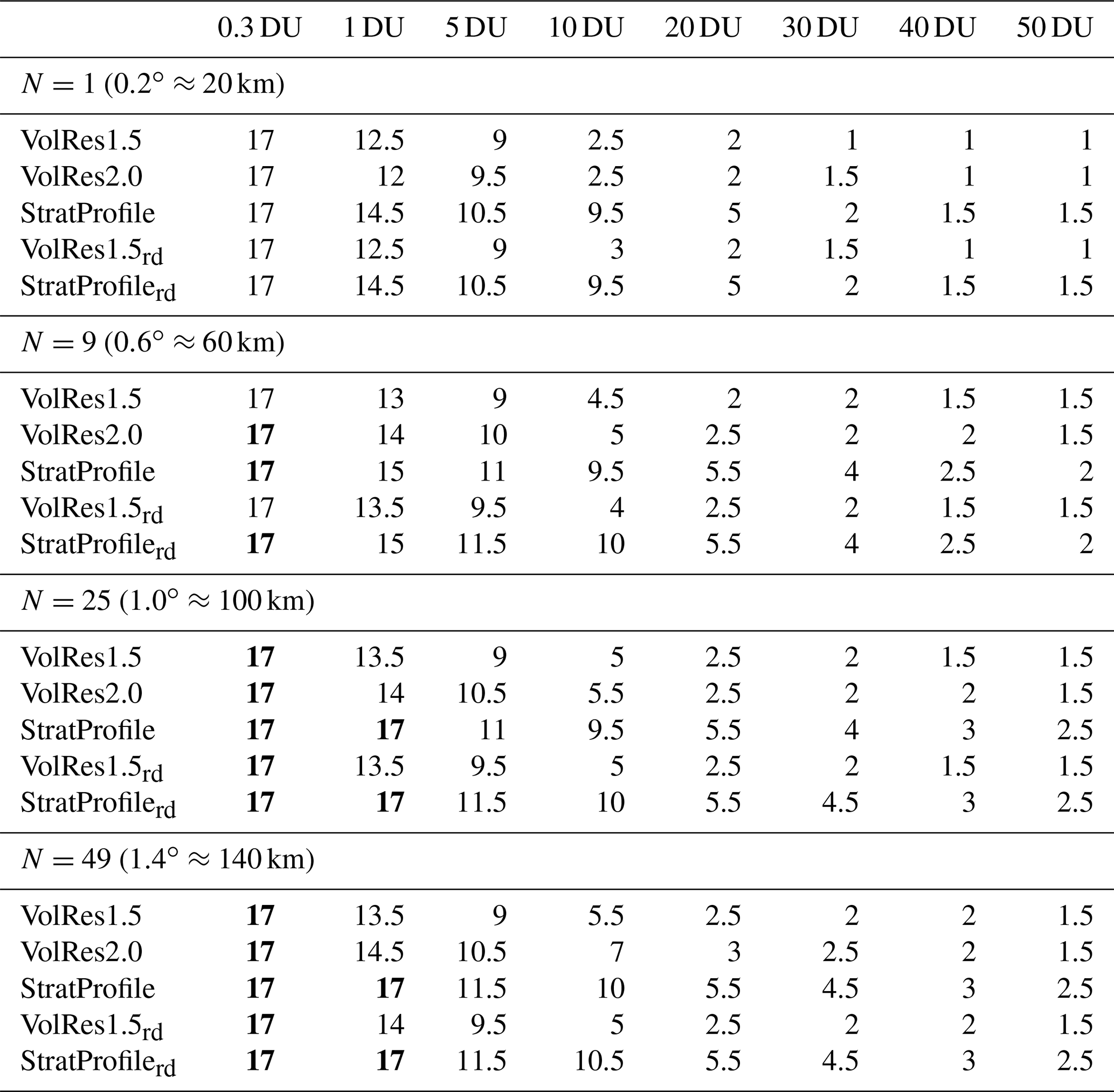
Code and simulation data used in this paper may be requested from the corresponding author and can be downloaded from https://doi.org/10.5281/zenodo.4729991 (de Leeuw, 2021). The TROPOMI satellite data can be downloaded from the ESA website (https://s5phub.copernicus.eu, last access: 9 December 2020) (Copernicus, 2020). Isabelle A. Taylor and Roy G. Grainger plan to archive the Oxford IASI SO2 products for the Raikoke eruption; in the meantime these can made available on request from Isabelle A. Taylor (isabelle.taylor@physics.ox.ac.uk). Radiosonde data are available at http://weather.uwyo.edu/upperair/sounding.html (Oolman, 2005). The NAME code is available under license from the Met Office.
Videos of the SO2 and SO4 NAME VCD simulations for the VolRes1.5 and the StratProfile emission profiles can be found at https://doi.org/10.5281/zenodo.3992052 (de Leeuw, 2020).
JdL, AS and CSW designed the project. JdL set up and performed all the NAME simulations and analysed the results. AS, CSW, MO and JH contributed to the scientific discussion and interpretation of the results. NK provided model input files for the initial NAME simulations. JdL, NT and RJP were responsible for the preparation of the TROPOMI data for the comparison with the NAME output. IT and RG processed the IASI data for the comparison. AS, CSW and RGG obtained the funding for this work. JdL, AS and CSW prepared the manuscript. All the authors reviewed the manuscript.
The authors declare that they have no conflict of interest.
This article is part of the special issue “Satellite observations, in situ measurements and model simulations of the 2019 Raikoke eruption (ACP/AMT/GMD inter-journal SI)”. It is not associated with a conference.
Johannes de Leeuw, Anja Schmidt, Claire S. Witham, Roy G. Grainger and Isabelle A. Taylor acknowledge funding from the Natural Environment Research Council (NERC) V-PLUS grants NE/S00436X/1 and NE/S004025/1. Isabelle A. Taylor and Roy G. Grainger are supported by the NERC Centre for Observation and Modelling of Earthquakes, Volcanoes, and Tectonics (COMET). Nicolas Theys acknowledges financial support from ESA S5P MPC (4000117151/16/I-LG) and Belgium Prodex TRACE-S5P (PEA 4000105598) projects. Funding for PhD work for Martin Osborne was provided by NERC through the University of Exeter, grant NE/M009416/1. Contributions from Jim Haywood and Anja Schmidt benefitted from support by the NERC ADVANCE (Aerosol-cloud-climate interactions derived from Degassing VolcANiC Eruptions), grant NE/T006897/1. The authors would like to thank Helen Webster (Met Office) for helpful discussions on the NAME diffusion parameterisations and Peter Haynes for our discussions on stratospheric mixing. We also like to acknowledge Andrew Prata and the anonymous reviewer for their comments and suggestions. This work used JASMIN, the UK collaborative data analysis facility (https://doi.org/10.1109/BigData.2013.6691556), to run all the simulations and to run the IASI SO2 retrieval. We would like to acknowledge EUMETSAT for providing the IASI spectra, as well as ECMWF and CEDA for the meteorological profiles used in the IASI retrievals (European Centre for Medium-Range Weather Forecasts, 2012).
This research has been supported by the Natural Environment Research Council (grant nos. NE/S00436X/1, NE/M009416/1, NE/T006897/1 and NE/S004025/1), ESA S5P MPC (grant no. 4000117151/16/I-LG) and Belgium Prodex TRACE-S5P (grant no. PEA 4000105598).
This paper was edited by Yves Balkanski and reviewed by Andrew Prata and one anonymous referee.
Abalos, M., Legras, B., and Shuckburgh, E.: Interannual variability in effective diffusivity in the upper troposphere/lower stratosphere from reanalysis data, Q. J. Roy. Meteorol. Soc., 142, 1847–1861, https://doi.org/10.1002/qj.2779, 2016. a
Allen, D. R. and Nakamura, N.: A seasonal climatology of effective diffusivity in the stratosphere, J. Geophys. Res.-Atmos., 106, 7917–7935, https://doi.org/10.1029/2000JD900717, 2001. a
Ashfold, M. J., Latif, M. T., Samah, A. A., Mead, M. I., and Harris, N. R. P.: Influence of Northeast Monsoon cold surges on air quality in Southeast Asia, Atmos. Environ., 166, 498–509, https://doi.org/10.1016/j.atmosenv.2017.07.047, 2017. a
Balluch, M. G. and Haynes, P. H.: Quantification of lower stratospheric mixing processes using aircraft data, J. Geophys. Res.-Atmos., 102, 23487–23504, https://doi.org/10.1029/97JD00607, 1997. a, b, c, d
Bernard, A. and Rose, W. I.: The injection of sulfuric acid aerosols in the stratosphere by the El Chichón volcano and its related hazards to the international air traffic, Nat. Hazards, 3, 59–67, https://doi.org/10.1007/BF00144974, 1990. a
Boichu, M., Menut, L., Khvorostyanov, D., Clarisse, L., Clerbaux, C., Turquety, S., and Coheur, P.-F.: Inverting for volcanic SO2 flux at high temporal resolution using spaceborne plume imagery and chemistry-transport modelling: the 2010 Eyjafjallajökull eruption case study, Atmos. Chem. Phys., 13, 8569–8584, https://doi.org/10.5194/acp-13-8569-2013, 2013. a, b
Brier, G. W.: Verification of forecasts expressed in terms of probability, Mon. Weather Rev., 78, 1–3, https://doi.org/10.1175/1520-0493(1950)078<0001:VOFEIT>2.0.CO;2, 1950. a
Bruckert, J., Hoshyaripour, G. A., Horváth, Á., Muser, L., Prata, F. J., Hoose, C., and Vogel, B.: Online treatment of eruption dynamics improves the volcanic ash and SO2 dispersion forecast: case of the Raikoke 2019 eruption, Atmos. Chem. Phys. Discuss. [preprint], https://doi.org/10.5194/acp-2021-459, in review, 2021. a, b
Bundke, U., Berg, M., Gomes, R., Haywood, J., Osborne, M., Schneider, J., Schulz, C., Hermann, M., Obersteiner, F., Gehrlein, T., Bönisch, H., Zahn, A., Vernier, J.-P., and Petzold, A.: Impact of the Raikoke volcanic eruption 2019 on the Northern Hemisphere UT/LS aerosol as seen from IAGOS-CARIBIC in-situ observations, in: European Aerosol Conference 2020, http://eac2020.de (last access: 30 April 2021), 2020. a
Carboni, E., Grainger, R., Walker, J., Dudhia, A., and Siddans, R.: A new scheme for sulphur dioxide retrieval from IASI measurements: application to the Eyjafjallajökull eruption of April and May 2010, Atmos. Chem. Phys., 12, 11417–11434, https://doi.org/10.5194/acp-12-11417-2012, 2012. a
Carboni, E., Grainger, R. G., Mather, T. A., Pyle, D. M., Thomas, G. E., Siddans, R., Smith, A. J. A., Dudhia, A., Koukouli, M. E., and Balis, D.: The vertical distribution of volcanic SO2 plumes measured by IASI, Atmos. Chem. Phys., 16, 4343–4367, https://doi.org/10.5194/acp-16-4343-2016, 2016. a, b, c, d, e
Carn, S. A., Krueger, A. J., Krotkov, N. A., Yang, K., and Evans, K.: Tracking volcanic sulfur dioxide clouds for aviation hazard mitigation, Nat. Hazards, 51, 325–343, https://doi.org/10.1007/s11069-008-9228-4, 2009. a
Carn, S. A., Clarisse, L., and Prata, A. J.: Multi-decadal satellite measurements of global volcanic degassing, J. Volcanol. Geoth. Res., 311, 99–134, https://doi.org/10.1016/j.jvolgeores.2016.01.002, 2016. a, b, c
Carpenter, L. J., Fleming, Z. L., Read, K. A., Lee, J. D., Moller, S. J., Hopkins, J. R., Purvis, R. M., Lewis, A. C., Müller, K., Heinold, B., Herrmann, H., Fomba, K. Wadinga, van Pinxteren, D., Müller, C., Tegen, I., Wiedensohler, A., Müller, T., Niedermeier, N., Achterberg, E. P., Patey, M. D., Kozlova, E. A., Heimann, M., Heard, D. E., Plane, J. M. C., Mahajan, A., Oetjen, H., Ingham, T., Stone, D., Whalley, L. K., Evans, M. J., Pilling, M. J., Leigh, R. J., Monks, P. S., Karunaharan, A., Vaughan, S., Arnold, S. R., Tschritter, J., Pöhler, D., Frieß, U., Holla, R., Mendes, L. M., Lopez, H., Faria, B., Manning, A. J., and Wallace, D. W. R: Seasonal characteristics of tropical marine boundary layer air measured at the Cape Verde Atmospheric Observatory, J. Atmos. Chem., 67, 87–140, https://doi.org/10.1007/s10874-011-9206-1, 2010. a
Casadevall, T. J., Reyes, P. J. D., and Schneider, D. J.: The 1991 Pinatubo eruptions and their effects on aircraft operations, in: Fire and Mud: Eruptions and Lahars of Mount Pinatubo, Philippines, Philippine Institute of Volcanology and Seismology, Quezon City, Philippines, 1996. a
Copernicus: Sentinel-5P Pro-Operations Data Hub, available at: https://s5phub.copernicus.eu, last access: 9 December 2020. a
Corradini, S., Merucci, L., and Folch, A.: Volcanic Ash Cloud Properties: Comparison Between MODIS Satellite Retrievals and FALL3D Transport Model, IEEE Geosci. Remote S., 8, 248–252, https://doi.org/10.1109/LGRS.2010.2064156, 2011. a
Crafford, A. and Venzke, E. (Eds.): Global Volcanism Program, Report on Raikoke (Russia), in: Bulletin of the Global Volcanism Network, Smithsonian Institution, Washington, D.C., USA, https://doi.org/10.5479/si.GVP.BGVN201908-290250, 2019. a, b
Dacre, H. F.: A new method for evaluating regional air quality forecasts, Atmos. Environ., 45, 993–1002, https://doi.org/10.1016/j.atmosenv.2010.10.048, 2011. a
Dacre, H. F. and Harvey, N. J.: Characterizing the Atmospheric Conditions Leading to Large Error Growth in Volcanic Ash Cloud Forecasts, J. Appl. Meteorol. Clim., 57, 1011–1019, https://doi.org/10.1175/JAMC-D-17-0298.1, 2018. a
Dacre, H. F., Grant, A. L. M., Harvey, N. J., Thomson, D. J., Webster, H. N., and Marenco, F.: Volcanic ash layer depth: Processes and mechanisms, Geophys. Res. Lett., 42, 637–645, https://doi.org/10.1002/2014GL062454, 2015. a
Dacre, H. F., Harvey, N. J., Webley, P. W., and Morton, D.: How accurate are volcanic ash simulations of the 2010 Eyjafjallajökull eruption?, J. Geophys. Res.-Atmos., 121, 3534–3547, https://doi.org/10.1002/2015JD024265, 2016. a
de Graaf, M., de Haan, J. F., and Sanders, A. F. J.: TROPOMI ATBD of the Aerosol Layer Height, available at: http://www.tropomi.eu/data-products/level-2-products (last access: 10 July 2020), 2016. a
de Leeuw, J.: Movie of the 2019 Raikoke volcanic eruption: Sulfur dioxide and sulfate dispersion as simulated by NAME [data set], Zenodo, https://doi.org/10.5281/zenodo.3992052, 2020. a, b
de Leeuw, J.: Data and software release related to paper discussing the 2019 Raikoke volcanic eruption (Version v1.0) [data set], Zenodo, https://doi.org/10.5281/zenodo.4729991, 2021. a
Dunn, M. G.: Operation of Gas Turbine Engines in an Environment Contaminated With Volcanic Ash, J. Turbomach., 134, 051001, https://doi.org/10.1115/1.4006236, 2012. a
Eckhardt, S., Prata, A. J., Seibert, P., Stebel, K., and Stohl, A.: Estimation of the vertical profile of sulfur dioxide injection into the atmosphere by a volcanic eruption using satellite column measurements and inverse transport modeling, Atmos. Chem. Phys., 8, 3881–3897, https://doi.org/10.5194/acp-8-3881-2008, 2008. a, b
Eliaz, N., Shemesh, G., and Latanision, R. M.: Hot corrosion in gas turbine components, Eng. Fail. Anal., 9, 31–43, 2002. a
European Centre for Medium-Range Weather Forecasts: ECMWF Operational Regular Gridded Data at 1.125 degrees resolution [data set], NCAS British Atmospheric Data Centre, available at: https://catalogue.ceda.ac.uk/uuid/a67f1b4d9db7b1528b800ed48198bdac (last access: 16 February 2021), 2012. a
Goitom, B., Oppenheimer, C., Hammond, J. O. S., Grandin, R., Barnie, T., Donovan, A., Ogubazghi, G., Yohannes, E., Kibrom, G., Kendall, J.-M., Carn, S. A., Fee, D., Sealing, C., Keir, D., Ayele, A., Blundy, J., Hamlyn, J., Wright, T., and Berhe, S.: First recorded eruption of Nabro volcano, Eritrea, 2011, B. Volcanol., 77, 85, https://doi.org/10.1007/s00445-015-0966-3, 2015. a
Gorkavyi, N., Krotkov, N., Li, C., Lait, L., Colarco, P., Carn, S., DeLand, M., Newman, P., Schoeberl, M., Taha, G., Torres, O., Vasilkov, A., and Joiner, J.: Tracking aerosols and SO2 clouds from the Raikoke eruption: 3D view from satellite observations, Atmos. Meas. Tech. Discuss. [preprint], https://doi.org/10.5194/amt-2021-58, in review, 2021. a
Granieri, D., Vita, F., and Inguaggiato, S.: Volcanogenic SO2, a natural pollutant: Measurements, modeling and hazard assessment at Vulcano Island (Aeolian Archipelago, Italy), Environ. Pollut., 231, 219–228, https://doi.org/10.1016/j.envpol.2017.07.101, 2017. a
Grégoire, B., Montero, X., Galetz, M. C., Bonnet, G., and Pedraza, F.: Mechanisms of hot corrosion of pure nickel at 700 ∘C: Influence of testing conditions, Corros. Sci., 141, 211–220, https://doi.org/10.1016/j.corsci.2018.06.009, 2018. a, b
Hamill, P., Toon, O. B., and Kiang, C. S.: Microphysical processes affecting stratospheric aerosol particles, J. Atmos. Sci., 34, 1104–1119, https://doi.org/10.1175/1520-0469(1977)034<1104:MPASAP>2.0.CO;2, 1977. a
Harvey, N. J. and Dacre, H. F.: Spatial evaluation of volcanic ash forecasts using satellite observations, Atmos. Chem. Phys., 16, 861–872, https://doi.org/10.5194/acp-16-861-2016, 2016. a, b
Harvey, N. J., Huntley, N., Dacre, H. F., Goldstein, M., Thomson, D., and Webster, H.: Multi-level emulation of a volcanic ash transport and dispersion model to quantify sensitivity to uncertain parameters, Nat. Hazards Earth Syst. Sci., 18, 41–63, https://doi.org/10.5194/nhess-18-41-2018, 2018. a, b, c, d, e, f
Haynes, P. and Anglade, J.: The Vertical-Scale Cascade in Atmospheric Tracers due to Large-Scale Differential Advection, J. Atmos. Sci., 54, 1121–1136, https://doi.org/10.1175/1520-0469(1997)054<1121:TVSCIA>2.0.CO;2, 1997. a, b
Haynes, P. and Shuckburgh, E.: Effective diffusivity as a diagnostic of atmospheric transport: 2. Troposphere and lower stratosphere, J. Geophys. Res.-Atmos., 105, 22795–22810, https://doi.org/10.1029/2000JD900092, 2000. a, b
Haywood, J. M., Jones, A., Clarisse, L., Bourassa, A., Barnes, J., Telford, P., Bellouin, N., Boucher, O., Agnew, P., Clerbaux, C., Coheur, P., Degenstein, D., and Braesicke, P.: Observations of the eruption of the Sarychev volcano and simulations using the HadGEM2 climate model, J. Geophys. Res.-Atmos., 115, D21212, https://doi.org/10.1029/2010JD014447, 2010. a, b
Heard, I. P. C., Manning, A. J., Haywood, J. M., Witham, C., Redington, A., Jones, A., Clarisse, L., and Bourassa, A.: A comparison of atmospheric dispersion model predictions with observations of SO2 and sulphate aerosol from volcanic eruptions, J. Geophys. Res.-Atmos., 117, D00U22, https://doi.org/10.1029/2011JD016791, 2012. a
Hedelt, P., Efremenko, D. S., Loyola, D. G., Spurr, R., and Clarisse, L.: Sulfur dioxide layer height retrieval from Sentinel-5 Precursor/TROPOMI using FP_ILM, Atmos. Meas. Tech., 12, 5503–5517, https://doi.org/10.5194/amt-12-5503-2019, 2019. a, b, c
Hegglin, M. I., Brunner, D., Peter, T., Staehelin, J., Wirth, V., Hoor, P., and Fischer, H.: Determination of eddy diffusivity in the lowermost stratosphere, Geophys. Res. Lett., 32, L13812, https://doi.org/10.1029/2005GL022495, 2005. a
Hofmann, D. J. and Rosen, J. M.: Stratospheric sulfuric acid fraction and mass estimate for the 1982 volcanic eruption of El Chichon, Geophys. Res. Lett., 10, 313–316, https://doi.org/10.1029/GL010i004p00313, 1983. a
Höpfner, M., Boone, C. D., Funke, B., Glatthor, N., Grabowski, U., Günther, A., Kellmann, S., Kiefer, M., Linden, A., Lossow, S., Pumphrey, H. C., Read, W. G., Roiger, A., Stiller, G., Schlager, H., von Clarmann, T., and Wissmüller, K.: Sulfur dioxide (SO2) from MIPAS in the upper troposphere and lower stratosphere 2002–2012, Atmos. Chem. Phys., 15, 7017–7037, https://doi.org/10.5194/acp-15-7017-2015, 2015. a
Hyman, D. M. and Pavolonis, M. J.: Probabilistic retrieval of volcanic SO2 layer height and partial column density using the Cross-track Infrared Sounder (CrIS), Atmos. Meas. Tech., 13, 5891–5921, https://doi.org/10.5194/amt-13-5891-2020, 2020. a
ICAO: Handbook on the international airways volcano watch (IAVW), available at: https://www.icao.int/airnavigation/METP/MOGVA Reference Documents/Handbook on the IAVW, Doc 9766.pdf (last access: 15 December 2019) 2019a. a
ICAO: Roadmap for International Airways Volcano Watch (IAVW) in Support of International Air Navigation, available at: https://www.icao.int/airnavigation/METP/MOGVA Reference Documents/IAVW Roadmap.pdf (last access: 15 December 2019), 2019b. a
Jégou, F., Berthet, G., Brogniez, C., Renard, J.-B., François, P., Haywood, J. M., Jones, A., Bourgeois, Q., Lurton, T., Auriol, F., Godin-Beekmann, S., Guimbaud, C., Krysztofiak, G., Gaubicher, B., Chartier, M., Clarisse, L., Clerbaux, C., Balois, J. Y., Verwaerde, C., and Daugeron, D.: Stratospheric aerosols from the Sarychev volcano eruption in the 2009 Arctic summer, Atmos. Chem. Phys., 13, 6533–6552, https://doi.org/10.5194/acp-13-6533-2013, 2013. a
Jones, A., Thomson, D., Hort, M., and Devenish, B.: The U.K. Met Office's Next-Generation Atmospheric Dispersion Model, NAME III, in: Air Pollution Modeling and Its Application XVII, Springer, Boston, Massachusetts, USA, 580–589, https://doi.org/10.1007/978-0-387-68854-1_62, 2007. a, b
Jones, A. C., Haywood, J. M., Jones, A., and Aquila, V.: Sensitivity of volcanic aerosol dispersion to meteorological conditions: A Pinatubo case study, J. Geophys. Res.-Atmos., 121, 6892–6908, https://doi.org/10.1002/2016JD025001, 2016. a
Karagulian, F., Clarisse, L., Clerbaux, C., Prata, A. J., Hurtmans, D., and Coheur, P. F.: Detection of volcanic SO2, ash, and H2SO4 using the Infrared Atmospheric Sounding Interferometer (IASI), J. Geophys. Res.-Atmos., 115, D00L02, https://doi.org/10.1029/2009JD012786, 2010. a
Katata, G., Chino, M., Kobayashi, T., Terada, H., Ota, M., Nagai, H., Kajino, M., Draxler, R., Hort, M. C., Malo, A., Torii, T., and Sanada, Y.: Detailed source term estimation of the atmospheric release for the Fukushima Daiichi Nuclear Power Station accident by coupling simulations of an atmospheric dispersion model with an improved deposition scheme and oceanic dispersion model, Atmos. Chem. Phys., 15, 1029–1070, https://doi.org/10.5194/acp-15-1029-2015, 2015. a
Kloss, C., Berthet, G., Sellitto, P., Ploeger, F., Taha, G., Tidiga, M., Eremenko, M., Bossolasco, A., Jégou, F., Renard, J.-B., and Legras, B.: Stratospheric aerosol layer perturbation caused by the 2019 Raikoke and Ulawun eruptions and their radiative forcing, Atmos. Chem. Phys., 21, 535–560, https://doi.org/10.5194/acp-21-535-2021, 2021. a, b, c
Klüser, L., Erbertseder, T., and Meyer-Arnek, J.: Observation of volcanic ash from Puyehue–Cordón Caulle with IASI, Atmos. Meas. Tech., 6, 35–46, https://doi.org/10.5194/amt-6-35-2013, 2013. a
Kooreman, M. L., Stammes, P., Trees, V., Sneep, M., Tilstra, L. G., de Graaf, M., Stein Zweers, D. C., Wang, P., Tuinder, O. N. E., and Veefkind, J. P.: Effects of clouds on the UV Absorbing Aerosol Index from TROPOMI, Atmos. Meas. Tech., 13, 6407–6426, https://doi.org/10.5194/amt-13-6407-2020, 2020. a
Kristiansen, N. I., Stohl, A., Prata, A. J., Richter, A., Eckhardt, S., Seibert, P., Hoffmann, A., Ritter, C., Bitar, L., Duck, T. J., and Stebel, K.: Remote sensing and inverse transport modeling of the Kasatochi eruption sulfur dioxide cloud, J. Geophys. Res.-Atmos., 115, D00L16, https://doi.org/10.1029/2009JD013286, 2010. a, b
Kristiansen, N. I., Prata, A. J., Stohl, A., and Carn, S. A.: Stratospheric volcanic ash emissions from the 13 February 2014 Kelut eruption, Geophys. Res. Lett., 42, 588–596, https://doi.org/10.1002/2014GL062307, 2015. a
Krotkov, N. A., Schoeberl, M. R., Morris, G. A., Carn, S., and Yang, K.: Dispersion and lifetime of the SO2 cloud from the August 2008 Kasatochi eruption, J. Geophys. Res.-Atmos., 115, D00L20, https://doi.org/10.1029/2010JD013984, 2010. a, b
Leadbetter, S. J., Hort, M. C., Jones, A. R., Webster, H. N., and Draxler, R. R.: Sensitivity of the modelled deposition of Caesium-137 from the Fukushima Dai-ichi nuclear power plant to the wet deposition parameterisation in NAME, J. Environ. Radioactiv., 139, 200–211, https://doi.org/10.1016/j.jenvrad.2014.03.018, 2015. a
Legras, B., Pisso, I., Berthet, G., and Lefèvre, F.: Variability of the Lagrangian turbulent diffusion in the lower stratosphere, Atmos. Chem. Phys., 5, 1605–1622, https://doi.org/10.5194/acp-5-1605-2005, 2005. a
Mateshvili, N., Fussen, D., Mateshvili, I., Vanhellemont, F., Bingen, C., Paatashvili, T., Kyrölä, E., Robert, C., and Dekemper, E.: Raikoke aerosol clouds observed from Tbilisi, Georgia and Halle, Belgium using ground-based twilight sky brightness spectral measurements., EGU General Assembly 2020, Online, 4–8 May 2020, EGU2020-7548, https://doi.org/10.5194/egusphere-egu2020-7548, 2020 a
Meyer, M., Burgin, L., Hort, M. C., Hodson, D. P., and Gilligan, C. A.: Large-scale atmospheric dispersal simulations identify likely airborne incursion routes of wheat stem rust into Ethiopia, Phytopathology, 107, 1175–1186, https://doi.org/10.1094/PHYTO-01-17-0035-FI, 2017. a
Miles, G. M., Grainger, R. G., and Highwood, E. J.: The significance of volcanic eruption strength and frequency for climate, Q. J. Roy. Meteorol. Soc., 130, 2361–2376, https://doi.org/10.1256/qj.03.60, 2004. a
Mittermaier, M., Roberts, N., and Thompson, S. A.: A long-term assessment of precipitation forecast skill using the Fractions Skill Score, Meteorol. Appl., 20, 176–186, https://doi.org/10.1002/met.296, 2013. a
Moxnes, E. D., Kristiansen, N. I., Stohl, A., Clarisse, L., Durant, A., Weber, K., and Vogel, A.: Separation of ash and sulfur dioxide during the 2011 Grímsvötn eruption, J. Geophys. Res.-Atmos., 119, 7477–7501, https://doi.org/10.1002/2013JD021129, 2014. a, b
Mulena, G. C., Allende, D. G., Puliafito, S. E., Lakkis, S. G., Cremades, P. G., and Ulke, A. G.: Examining the influence of meteorological simulations forced by different initial and boundary conditions in volcanic ash dispersion modelling, Atmos. Res., 176–177, 29–42, https://doi.org/10.1016/j.atmosres.2016.02.009, 2016. a
Muser, L. O., Hoshyaripour, G. A., Bruckert, J., Horváth, Á., Malinina, E., Wallis, S., Prata, F. J., Rozanov, A., von Savigny, C., Vogel, H., and Vogel, B.: Particle aging and aerosol–radiation interaction affect volcanic plume dispersion: evidence from the Raikoke 2019 eruption, Atmos. Chem. Phys., 20, 15015–15036, https://doi.org/10.5194/acp-20-15015-2020, 2020. a, b, c, d, e, f
National Research Council Committee: Acute Exposure Guideline Levels for Selected Airborne Chemicals: Sulfur Dioxide Acute Exposure Guideline Levels, available at: https://www.ncbi.nlm.nih.gov/books/NBK219999/, last access: 14 July 2020. a
Niemeier, U., Timmreck, C., Graf, H.-F., Kinne, S., Rast, S., and Self, S.: Initial fate of fine ash and sulfur from large volcanic eruptions, Atmos. Chem. Phys., 9, 9043–9057, https://doi.org/10.5194/acp-9-9043-2009, 2009. a
Oolman, L.: Atmospheric Soundings, University of Wyoming, available at: http://weather.uwyo.edu/upperair/sounding.html (last access: 6 July 2021), 2005. a
Oppenheimer, C., Scaillet, B., and Martin, R. S.: Sulfur Degassing From Volcanoes: Source Conditions, Surveillance, Plume Chemistry and Earth System Impacts, Rev. Mineral. Geochem., 73, 363–421, https://doi.org/10.2138/rmg.2011.73.13, 2011. a
Osborne, M., Malavelle, F. F., Adam, M., Buxmann, J., Sugier, J., Marenco, F., and Haywood, J.: Saharan dust and biomass burning aerosols during ex-hurricane Ophelia: observations from the new UK lidar and sun-photometer network, Atmos. Chem. Phys., 19, 3557–3578, https://doi.org/10.5194/acp-19-3557-2019, 2019. a
Osborne, M. J., de Leeuw, J., Witham, C., Schmidt, A., Beckett, F., Kristiansen, N., Buxmann, J., Saint, C., Welton, E. J., Fochesatto, J., Gomes, A. R., Bundke, U., Petzold, A., Marenco, F., and Haywood, J.: The 2019 Raikoke volcanic eruption part 2: Particle phase dispersion and concurrent wildfire smoke emissions, Atmos. Chem. Phys. Discuss. [preprint], https://doi.org/10.5194/acp-2021-448, in review, 2021. a, b, c, d, e
Pardini, F., Burton, M., Arzilli, F., La Spina, G., and Polacci, M.: SO2 emissions, plume heights and magmatic processes inferred from satellite data: The 2015 Calbuco eruptions, J. Volcanol. Geoth. Res., 361, 12–24, https://doi.org/10.1016/j.jvolgeores.2018.08.001, 2018. a
Pfeffer, M. A., Bergsson, B., Barsotti, S., Stefánsdóttir, G., Galle, B., Arellano, S., Conde, V., Donovan, A., Ilyinskaya, E., Burton, M., Aiuppa, A., Whitty, R. C. W., Simmons, I. C., Arason, P., Jónasdóttir, E. B., Keller, N. S., Yeo, R. F., Arngrímsson, H., Jóhannsson, P., Butwin, M. K., Askew, R. A., Dumont, S., Von Löwis, S., Ingvarsson, P., La Spina, A., Thomas, H., Prata, F., Grassa, F., Giudice, G., Stefánsson, A., Marzano, F., Montopoli, M., and Mereu, L.: Ground-Based Measurements of the 2014–2015 Holuhraun Volcanic Cloud (Iceland), Geosciences, 8, 29, https://doi.org/10.3390/geosciences8010029, 2018. a
Platt, U. and Stutz, J.: Differential Optical Absorption Spectroscopy (DOAS): Principle and Applications, Springer, Berlin, Germany, 2008. a
Prata, A. J. and Prata, A. T.: Eyjafjallajökull volcanic ash concentrations determined using Spin Enhanced Visible and Infrared Imager measurements, J. Geophys. Res.-Atmos., 117, D00U23, https://doi.org/10.1029/2011JD016800, 2012. a
Prata, A. J. and Tupper, A.: Aviation hazards from volcanoes: the state of the science, Nat. Hazards, 51, 239–244, 2009. a
Prata, A. T., Dacre, H. F., Irvine, E. A., Mathieu, E., Shine, K. P., and Clarkson, R. J.: Calculating and communicating ensemble-based volcanic ash dosage and concentration risk for aviation, Meteorol. Appl., 26, 253–266, https://doi.org/10.1002/met.1759, 2019. a
Prata, A. T., Mingari, L., Folch, A., Macedonio, G., and Costa, A.: FALL3D-8.0: a computational model for atmospheric transport and deposition of particles, aerosols and radionuclides – Part 2: Model validation, Geosci. Model Dev., 14, 409–436, https://doi.org/10.5194/gmd-14-409-2021, 2021. a, b
Pyle, D. M.: Mass and energy budgets of explosive volcanic eruptions, Geophys. Res. Lett., 22, 563–566, https://doi.org/10.1029/95GL00052, 1995. a
Radanovics, S., Vidal, J.-P., and Sauquet, E.: Spatial verification of ensemble precipitation: an ensemble version of SAL, Weather Forecast., 33, 1001–1020, https://doi.org/10.1175/WAF-D-17-0162.1, 2018. a
Redington, A. L., Derwent, R. G., Witham, C. S., and Manning, A. J.: Sensitivity of modelled sulphate and nitrate aerosol to cloud, pH and ammonia emissions, Atmos. Environ., 43, 3227–3234, https://doi.org/10.1016/j.atmosenv.2009.03.041, 2009. a
Rix, M., Valks, P., Hao, N., van Geffen, J., Clerbaux, C., Clarisse, L., Coheur, P.-F., Loyola, R., Diego, G., Erbertseder, T., Zimmer, W., and Emmadi, S.: Satellite Monitoring of Volcanic Sulfur Dioxide Emissions for Early Warning of Volcanic Hazards, IEEE J. Sel. Top. Appl., 2, 196–206, https://doi.org/10.1109/JSTARS.2009.2031120, 2009. a
Roberts, N.: Assessing the spatial and temporal variation in the skill of precipitation forecasts from an NWP model, Meteorol. Appl., 15, 163–169, https://doi.org/10.1002/met.57, 2008. a
Roberts, N. M. and Lean, H. W.: Scale-selective verification of rainfall accumulations from high-resolution forecasts of convective events, Mon. Weather Rev., 136, 78–97, https://doi.org/10.1175/2007MWR2123.1, 2008. a
Robock, A.: Volcanic eruptions and climate, Rev. Geophys., 38, 191–219, https://doi.org/10.1029/1998RG000054, 2000. a
Sahyoun, M., Freney, E., Brito, J., Duplissy, J., Gouhier, M., Colomb, A., Dupuy, R., Bourianne, T., Nowak, J. B., Yan, C., Petäjä, T., Kulmala, M., Schwarzenboeck, A., Planche, C., and Sellegri, K.: Evidence of New Particle Formation Within Etna and Stromboli Volcanic Plumes and Its Parameterization From Airborne In Situ Measurements, J. Geophys. Res.-Atmos., 124, 5650–5668, https://doi.org/10.1029/2018JD028882, 2019. a
Schmidt, A., Ostro, B., Carslaw, K. S., Wilson, M., Thordarson, T., Mann, G. W., and Simmons, A. J.: Excess mortality in Europe following a future Laki-style Icelandic eruption, P. Natl. Acad. Sci. USA, 108, 15710–15715, https://doi.org/10.1073/pnas.1108569108, 2011. a
Schmidt, A., Carslaw, K. S., Mann, G. W., Rap, A., Pringle, K. J., Spracklen, D. V., Wilson, M., and Forster, P. M.: Importance of tropospheric volcanic aerosol for indirect radiative forcing of climate, Atmos. Chem. Phys., 12, 7321–7339, https://doi.org/10.5194/acp-12-7321-2012, 2012. a
Schmidt, A., Witham, C. S., Theys, N., Richards, N. A. D., Thordarson, T., Szpek, K., Feng, W., Hort, M. C., Woolley, A. M., Jones, A. R., Redington, A. L., Johnson, B. T., Hayward, C. L., and Carslaw, K. S.: Assessing hazards to aviation from sulfur dioxide emitted by explosive Icelandic eruptions, J. Geophys. Res.-Atmos., 119, 14–180, https://doi.org/10.1002/2014JD022070, 2014. a, b
Schmidt, A., Leadbetter, S., Theys, N., Carboni, E., Witham, C. S., Stevenson, J. A., Birch, C. E., Thordarson, T., Turnock, S., Barsotti, S., Delaney, L., Feng, W., Grainger, R. G., Hort, M. C., Höskuldsson, Á., Ialongo, I., Ilyinskaya, E., Jóhannsson, T., Kenny, P., Mather, T. A., Richards, N. A. D., and Shepherd, J.: Satellite detection, long-range transport, and air quality impacts of volcanic sulfur dioxide from the 2014–2015 flood lava eruption at Bárðarbunga (Iceland), J. Geophys. Res.-Atmos., 120, 9739–9757, https://doi.org/10.1002/2015JD023638, 2015. a, b
Schmidt, A., Mills, M. J., Ghan, S., Gregory, J. M., Allan, R. P., Andrews, T., Bardeen, C. G., Conley, A., Forster, P. M., Gettelman, A., Portmann, R. W., Solomon, S., and Toon, O. B.: Volcanic radiative forcing from 1979 to 2015, J. Geophys. Res.-Atmos., 123, 12491–12508, https://doi.org/10.1029/2018JD028776, 2018. a, b, c
Sears, T. M., Thomas, G. E., Carboni, E., Smith, A. J., and Grainger, R. G.: SO2 as a possible proxy for volcanic ash in aviation hazard avoidance, J. Geophys. Res.-Atmos., 118, 5698–5709, https://doi.org/10.1002/jgrd.50505, 2013. a
Shindell, D. T., Schmidt, G. A., Mann, M. E., and Faluvegi, G.: Dynamic winter climate response to large tropical volcanic eruptions since 1600, J. Geophys. Res.-Atmos., 109, D05104, https://doi.org/10.1029/2003JD004151, 2004. a
Solomon, S., Daniel, J. S., Neely, R. R., Vernier, J.-P., Dutton, E. G., and Thomason, L. W.: The persistently variable “background” stratospheric aerosol layer and global climate change, Science, 333, 866–870, https://doi.org/10.1126/science.1206027, 2011. a
Stenchikov, G.: The Role of Volcanic Activity in Climate and Global Change, 2nd Edn., Elsevier, Boston, Massachusetts, USA, https://doi.org/10.1016/B978-0-444-63524-2.00026-9, 2016. a
Theys, N., De Smedt, I., Yu, H., Danckaert, T., van Gent, J., Hörmann, C., Wagner, T., Hedelt, P., Bauer, H., Romahn, F., Pedergnana, M., Loyola, D., and Van Roozendael, M.: Sulfur dioxide retrievals from TROPOMI onboard Sentinel-5 Precursor: algorithm theoretical basis, Atmos. Meas. Tech., 10, 119–153, https://doi.org/10.5194/amt-10-119-2017, 2017. a, b, c, d, e
Theys, N., Lerot, C., Van Roozendael, M., De Smedt, I., and Yu, H.: S5P ATBD of the Sulfur dioxide product, available at: http://www.tropomi.eu/data-products/level-2-products (last access: 17 December 2019), 2018. a, b, c
Theys, N., Hedelt, P., De Smedt, I., Lerot, C., Yu, H., Vlietinck, J., Pedergnana, M., Arellano, S., Galle, B., Fernandez, D., Carlito, C. J. M., Barrington, C., Taisne, B., Delgado-Granados, H., Loyola, D., and Van Roozendael, M.: Global monitoring of volcanic SO2 degassing with unprecedented resolution from TROPOMI onboard Sentinel-5 Precursor, Sci. Rep.-UK, 9, 2643, https://doi.org/10.1038/s41598-019-39279-y, 2019. a, b, c, d
Theys, N., Romahn, F., and Wagner, T.: S5P Mission Performance Centre Sulphur Dioxide Readme, available at: https://sentinel.esa.int/documents/247904/3541451/Sentinel-5P-Sulphur-Dioxide-Readme.pdf, last access: 8 December 2020. a
Thomas, H. E. and Prata, A. J.: Sulphur dioxide as a volcanic ash proxy during the April–May 2010 eruption of Eyjafjallajökull Volcano, Iceland, Atmos. Chem. Phys., 11, 6871–6880, https://doi.org/10.5194/acp-11-6871-2011, 2011. a
Trenberth, K. E. and Dai, A.: Effects of Mount Pinatubo volcanic eruption on the hydrological cycle as an analog of geoengineering, Geophys. Res. Lett., 34, L15702, https://doi.org/10.1029/2007GL030524, 2007. a
Vaughan, G., Wareing, D., and Ricketts, H.: Lidar observations of volcanic aerosol over the UK since June 2019, EGU General Assembly 2020, Online, 4–8 May 2020, EGU2020-5653, https://doi.org/10.5194/egusphere-egu2020-5653, 2020. a
Veefkind, J. P., Aben, I., McMullan, K., Förster, H., de Vries, J., Otter, G., Claas, J., Eskes, H. J., de Haan, J. F., Kleipool, Q., van Weele, M., Hasekamp, O., Hoogeveen, R., Landgraf, J., Snel, R., Tol, P., Ingmann, P., Voors, R., Kruizinga, B., Vink, R., Visser, H., and Levelt, P. F.: TROPOMI on the ESA Sentinel-5 Precursor: A GMES mission for global observations of the atmospheric composition for climate, air quality and ozone layer applications, Remote Sens. Environ., 120, 70–83, https://doi.org/10.1016/j.rse.2011.09.027, 2012. a
Vira, J., Carboni, E., Grainger, R. G., and Sofiev, M.: Variational assimilation of IASI SO2 plume height and total column retrievals in the 2010 eruption of Eyjafjallajökull using the SILAM v5.3 chemistry transport model, Geosci. Model Dev., 10, 1985–2008, https://doi.org/10.5194/gmd-10-1985-2017, 2017. a
Wang, Z., Hase, N., Notholt, J., Dils, B., Saunois, M., Warneke, T., and Tian, W.: Diagnosing Mixing Properties in Model Simulations for CH4 in the Stratosphere, J. Geophys. Res.-Atmos., 125, e2020JD032524, https://doi.org/10.1029/2020JD032524, 2020. a, b
Waugh, D. W., Plumb, R. A., Elkins, J. W., Fahey, D. W., Boering, K. A., Dutton, G. S., Volk, C. M., Keim, E., Gao, R.-S., Daube, B. C., Wofsy, S. C., Loewenstein, M., Podolske, J. R., Chan, K. R., Proffitt, M. H., Kelly, K. K., Newman, P. A., and Lait, L. R.: Mixing of polar vortex air into middle latitudes as revealed by tracer-tracer scatterplots, J. Geophys. Res.-Atmos., 102, 13119–13134, https://doi.org/10.1029/96JD03715, 1997. a, b, c, d
Webster, H. and Thomson, D.: The NAME wet deposition scheme, Technical Report No. 584, Met Office, Forecasting Research Division, Exeter, available at: https://library.metoffice.gov.uk/Portal/Default/en-GB/RecordView/Index/197129 (last access: 7 July 2021), 2014. a
Webster, H. N., Devenish, B. J., Haywood, J. M., Lock, A. P., and Thomson, D. J.: Using plume rise schemes to model highly buoyant plumes from large fires, Int. J. Environ. Pollut., 44, 226–234, https://doi.org/10.1504/IJEP.2011.038422, 2011. a
Webster, H. N., Whitehead, T., and Thomson, D.: Parameterizing Unresolved Mesoscale Motions in Atmospheric Dispersion Models, J. Appl. Meteorol. Clim., 57, 645–657, https://doi.org/10.1175/JAMC-D-17-0075.1, 2018. a, b, c, d, e
Webster, H. N., Devenish, B. J., Mastin, L. G., Thomson, D. J., and Van Eaton, A. R.: Operational Modelling of Umbrella Cloud Growth in a Lagrangian Volcanic Ash Transport and Dispersion Model, Atmosphere, 11, 200, https://doi.org/10.3390/atmos11020200, 2020. a
Wernli, H., Paulat, M., Hagen, M., and Frei, C.: SAL – A novel quality measure for the verification of quantitative precipitation forecasts, Mon. Weather Rev., 136, 4470–4487, https://doi.org/10.1175/2008MWR2415.1, 2008. a, b, c
Whitty, R. C. W., Ilyinskaya, E., Mason, E., Wieser, P. E., Liu, E. J., Schmidt, A., Roberts, T., Pfeffer, M. A., Brooks, B., Mather, T. A., Edmonds, M., Elias, T., Schneider, D. J., Oppenheimer, C., Dybwad, A., Nadeau, P. A., and Kern, C.: Spatial and Temporal Variations in SO2 and PM2.5 Levels Around Kīlauea Volcano, Hawai'i During 2007–2018, Front. Earth Sci., 8, 36, https://doi.org/10.3389/feart.2020.00036, 2020. a
Wilkins, K. L., Watson, I. M., Kristiansen, N. I., Webster, H. N., Thomson, D. J., Dacre, H. F., and Prata, A. J.: Using data insertion with the NAME model to simulate the 8 May 2010 Eyjafjallajökull volcanic ash cloud, J. Geophys. Res.-Atmos., 121, 306–323, https://doi.org/10.1002/2015JD023895, 2016. a, b
Witham, C., Webster, H., Hort, M., Jones, A., and Thomson, D.: Modelling concentrations of volcanic ash encountered by aircraft in past eruptions, Atmos. Environ., 48, 219–229, https://doi.org/10.1016/j.atmosenv.2011.06.073, 2012. a
Witham, C., Hort, M., Thomson, D., Leadbetter, S., Devenish, B., Webster, H., Beckett, F., and Kristiansen, N.: The current volcanic ash modelling set-up at the London VAAC Technical Summary (v1.6), available at: https://www.metoffice.gov.uk/binaries/content/assets/metofficegovuk/pdf/services/transport/aviation/vaac/london_vaac_current_modelling_setup_jan20.pdf, last access: 27 July 2020. a
Witham, C. S., Hort, M. C., Potts, R., Servranckx, R., Husson, P., and Bonnardot, F.: Comparison of VAAC atmospheric dispersion models using the 1 November 2004 Grimsvötn eruption, Meteorol. Appl., 14, 27–38, https://doi.org/10.1002/met.3, 2007. a
Yang, K., Liu, X., Bhartia, P. K., Krotkov, N. A., Carn, S. A., Hughes, E. J., Krueger, A. J., Spurr, R. J., and Trahan, S. G.: Direct retrieval of sulfur dioxide amount and altitude from spaceborne hyperspectral UV measurements: Theory and application, J. Geophys. Res.-Atmos., 115, D00L09, https://doi.org/10.1029/2010JD013982, 2010. a, b
Zweers, S.: TROPOMI ATBD of the UV aerosol index, available at: http://www.tropomi.eu/data-products/level-2-products (last access: 10 July 2020, 2016. a
- Abstract
- Introduction
- Data and methods
- Results
- Discussion
- Conclusions
- Appendix A: Derivation of StratProfile vertical emission profile
- Code and data availability
- Video supplement
- Author contributions
- Competing interests
- Special issue statement
- Acknowledgements
- Financial support
- Review statement
- References