The 2019 Raikoke volcanic eruption – Part 2: Particle-phase dispersion and concurrent wildfire smoke emissions

Between 27 June and 14 July 2019 aerosol layers were observed by the United Kingdom (UK) Raman lidar network in the upper troposphere and lower stratosphere. The arrival of these aerosol layers in late June caused some concern within the London Volcanic Ash Advisory Centre (VAAC) as according to dispersion simulations the volcanic plume from the 21 June 2019 eruption of Raikoke was not expected over the UK until early July. Using dispersion simulations from the Met Office Numerical Atmospheric-dispersion Modelling Environment (NAME), and supporting evidence from satellite and in situ aircraft observations, we show that the early arrival of the stratospheric layers was not due to aerosols from the explosive eruption of the Raikoke volcano but due to biomass burning smoke aerosols associated with intense forest fires in Alberta, Canada, that occurred 4 d prior to the Raikoke eruption. We use the observations and model simulations to describe the dispersion of both the volcanic and forest fire aerosol clouds and estimate that the initial Raikoke ash aerosol cloud contained around 15 Tg of volcanic ash and that the forest fires produced around 0.2 Tg of biomass burning aerosol. The operational monitoring of volcanic aerosol clouds is a vital capability in terms of aviation safety and the synergy of NAME dispersion simulations, and lidar data with depolarising capabilities allowed scientists at the Met Office to interpret the various aerosol layers over the UK and attribute the material to their sources. The use of NAME allowed the identification of the observed stratospheric layers that reached the UK on 27 June as biomass burning aerosol, characterised by a particle linear depolarisation ratio of 9 %, whereas with the lidar alone the latter could have been identified as the early arrival of a volcanic ash–sulfate mixed aerosol cloud. In the case under study, given the low concentration estimates, the exact identification of the aerosol layers would have made little substantive difference to the decision-making process within the London VAAC. However, our work shows how the use of dispersion modelling together with multiple observation sources enabled us to create a more complete description of atmospheric aerosol loading.

1 Introduction

Explosive volcanic eruptions can inject volcanic ash and sulfur dioxide (SO₂) into the stratosphere that can have residence times of many months or even years (e.g. Langmann, 2014; Carn et al., 2017). The dangers and disruption presented to aviation by volcanic ash aerosol clouds have been well documented and can be present even far from the emitting volcano when long-range transport takes place (e.g. Guffanti et al., 2010; Gordeev, 2014). Of particular concern to the aviation community is that volcanic ash melts in the high-temperature chambers within jet engines, coating the turbines, and, in high enough concentrations, can cause the engine to stall with no guarantee of it restarting (Miller and Casadeval, 1999). Volcanic aerosol clouds containing SO₂ and/or sulfuric acid droplets have the potential to damage aircraft windows and cause distress to passengers and crew (Bernard and Rose, 1990). The damage to engines and airframes resulting from an aircraft encountering volcanic aerosol clouds can cause significant costs to airlines, with a single encounter potentially costing tens of millions of Euros (Miller and Casadeval, 1999; Prata and Tupper, 2009). Another impact of volcanic ash clouds (and also of desert dust layers) on aviation is the effect of these aerosol layers on visibility from a pilot's perspective (Weinzierl et al., 2012). Precautionary regulatory measures resulting from volcanic activity, while necessary for public safety, can have far reaching impacts on the entire industry. For example, the 2010 eruption of the Icelandic volcano Eyjafjallajökull caused widespread disruption to air travel across Europe for several weeks and had a significant financial impact on several large airlines (Gertisser, 2010). To mitigate these risks the International Civil Aviation Authority designates nine centres to act as Volcanic Ash Advisory Centres (VAACs), each of which is responsible for issuing warnings and information to national aviation authorities and the wider aviation community. The Met Office acts as the London VAAC and formulates guidance products using a combination of dispersion model simulations (Jones et al., 2007; Webster et al., 2012; Dacre et al., 2015), satellite observations (Millington et al., 2012; Francis et al., 2012), and ground-based and aircraft observations (Turnbull et al., 2012; Marenco et al., 2016; Osborne et al., 2019).

Biomass burning aerosol (BBA) can also be injected to aircraft flight altitudes (e.g. Fromm et al., 2005, 2006; Christian et al., 2019; Khaykin et al., 2020) but has received far less attention from the aviation community, as it does not have a direct potential for damaging aircraft. BBA can however cause disruption to aviation as the characteristic burning smell can be misidentified as originating from the aircraft, causing activation of emergency procedures. For example, in October 2017, 32 emergency procedure and MAYDAY calls from aircraft in UK airspace were received owing to reports of smoke within the cabin leading to emergency descents, emergency landings and emergency evacuations, which caused much passenger distress and displacement of passengers and aircraft. Studies of this event have revealed that there were unusually high concentrations of BBA in UK airspace that had been transported from fires on the Iberian Peninsula by the synoptic large-scale transport associated with Hurricane Ophelia (Osborne et al., 2019).

As part of its ground-based volcanic ash remote-sensing capability, the Met Office operates a network of 10 single-wavelength, ground-based Raman lidars distributed across the UK. The installations also have co-located AERONET sun photometers (Adam et al., 2017; Osborne et al., 2019). Active laser remote sensing using lidars is well suited to the task of detecting aerosol and cloud layers and providing quantitative estimates of concentrations as it provides atmospheric profiles that are highly resolved in both altitude and time. Lidar networks, e.g. NASA MPLNET (Micro-Pulse Lidar Network), EARLINET (European Aerosol Research Lidar Network) and LALINET (Latin America Lidar Network) (Welton et al., 2001; Pappalardo et al., 2014; Guerrero-Rascado et al., 2016; Lewis et al., 2016), can also provide coverage over a wide geographical area and can be used to track the progress and evolution of aerosol clouds. By using lidars equipped with a Raman channel as well as depolarisation discrimination, aerosol type identification can be attempted as well as the estimation of separate mass profiles for depolarising and non-depolarising aerosols (e.g. Ansmann et al., 1992; Webley et al., 2008; Tesche et al., 2009; Groß et al., 2015a). However, aerosol identification made using these methods can sometimes be ambiguous, and it is useful to use additional information to try and reach a more certain identification. Dispersion model simulations and subsequent source attribution frequently offer a good chance of arriving at an unambiguous aerosol classification. The Met Office has developed and maintains a world-leading atmospheric-dispersion model, NAME (Jones et al., 2007). In addition to its role as an emergency response guidance tool, the model is used for routine air quality forecasting and meteorological research activities.

In late June and early July 2019 aerosol layers were observed in the upper troposphere and lower stratosphere (UTLS) by several lidars in the UK, including those in the Met Office network (Vaughan et al., 2021). While dispersion modelling performed at the time suggested that aerosols from the eruption of the Raikoke volcano on 21 June 2019 would reach the UK by early July 2019, the arrival of aerosol layers in the UTLS in late June caused some surprise. The depolarisation ratio measurement of 9 % in these initial layers meant that the Raikoke eruption could not be ruled out as a possible source using this evidence alone. While depolarisation ratios for volcanic ash are often found to be greater than 30 % and those for volcanic sulfate aerosols are expected to be around 1 % (e.g. Illingworth et al., 2015), an external mixture of the two aerosols could produce an overall particle depolarisation ratio of around 9 % (Groß et al., 2011).

This paper forms the second part of a two-part study. In part one, de Leeuw et al. (2021) describe the transport and chemical evolution of the gas-phase emissions from the 2019 Raikoke eruption and provide a detailed comparison of NAME model simulations with observations from the TROPOspheric Monitoring Instrument (TROPOMI) on board the European Space Agency Sentinel-5P satellite. Here, we focus on the transport and evolution of the particle phase of the Raikoke volcanic emissions together with the transport of particulate material from fires in Alberta, Canada. For consistency with the study of de Leeuw et al. (2021), we use the term aerosol cloud to represent the area influenced by volcanic and BBA aerosols. We acknowledge that this is not technically meteorologically correct as meteorological clouds are formed of droplets of condensed water vapour, but we maintain this terminology for consistency between the two studies.

In Sect. 2 of this paper, we briefly describe the Raikoke eruption and concurrent relevant intense forest fires, and then in Sect. 3 we describe how the NAME model simulations were initialised, as well as a brief description of the observation data and various instruments used in this study. In Sect. 4 we present the results, concentrating first on the geographic distribution and vertical structure of volcanic aerosols and then on the geographic distribution and vertical structure of BBA with additional regional analyses over North America and over the UK. Section 5 provides some conclusions.

2 Raikoke eruption and wildfires in summer 2019

Over the course of 21 and 22 June 2019, the Raikoke volcano located in the Kuril archipelago in the north-west Pacific erupted explosively, injecting ash and SO₂ into the upper troposphere and lower stratosphere. At approximately 1.5±0.2 Tg of SO₂ (Crafford and Venzke, 2019; de Leeuw et al., 2021) this emission is of similar magnitude to the eruptions of Kasatochi in August 2008 (Kravitz et al., 2010), Sarychev in June 2009 (Haywood et al., 2010) and Nabro in June 2011 (Clarisse et al., 2012). Satellite imagery of the plume indicates that the eruption was ash-rich in nature, and estimates of the emission are derived in Sect. 3.1.

The 2019 wildfire season in the Canadian province of Alberta was unusually severe, with more than 883 000 ha burned across the province, compared to the 2014 to 2018 5-year average of 245 000 ha, and the largest area burned since 1981 (Short, 2019a; Jenner, 2019; Gabbert, 2019). The Mackenzie County area in the north of Alberta suffered a particularly large number of fires in May and June 2019, resulting in the evacuation of thousands of people and the destruction of property (Short, 2019b). Continued hot and dry conditions along with high winds caused intensification of the wildfires; the heat released fuelled pyrocumulus clouds, which lofted smoke into the UTLS and allowed high-level winds to transport it long distances. On 17 June 2019, 4 d prior to the eruption of Raikoke, wildfires burning in Chuckegg Creek in Mackenzie County produced biomass burning aerosols and formed pyrocumulus clouds which breached the tropopause and entered the lower stratosphere. Figure 1a shows a true colour reflectance MODIS image from the 17 June 2019 overlaid with thermal anomalies associated with forest fires; an aerosol cloud can clearly be seen to have moved north-eastwards from an area with several active fires. We will show that the aerosol cloud continued eastwards over the following days, with the lower tropospheric layers moving south over the United States and the stratospheric layers continuing eastwards to reach Europe by 26 June.

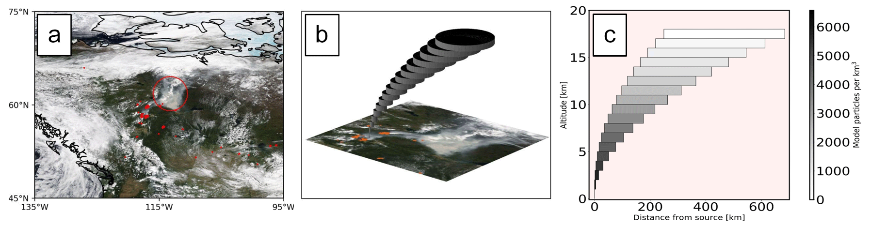
Figure 1 (a) MODIS Terra true colour reflectance tile for 17 June 2019 with thermal anomalies overlaid in red. Emissions from forest fires can be seen as a brownish grey cloud (circled in red). (b) Conceptual diagram of NAME source term used to initialise BBA dispersion simulation. (c) Profile of source term showing the concentration of model particles in each cylinder. Within each cylinder an arbitrary mass of 0.1 Tg was released over 100 000 model particles uniformly distributed through the volume of each cylinder.

3 Methods

3.1 NAME dispersion model simulations

The dispersion of gas and aerosols is simulated within NAME by tracking notional “particles” as they move within air parcels advected by the wind vectors supplied by a driving meteorological model. Operationally the Met Office Unified Model (UM) version 7.1 (Walters et al., 2019) provides the global driving meteorology with a 3-hourly temporal resolution and approximately 10 km horizontal resolution at mid-latitudes, as well as on 59 model levels between the surface and 30 km altitude. Turbulence and sub-grid-scale diffusion are represented within NAME by the addition of random perturbations to the wind vectors at each time step (Webster et al., 2012). de Leeuw et al. (2021) perform a detailed quantitative investigation of the effect of this diffusion parameter on the spatial extent and concentration of the diffused volcanic SO₂ cloud. For the Raikoke eruption, de Leeuw et al. (2021) obtained better agreement between the simulated and observed SO₂ clouds by using a reduced parameterisation of sub-grid-scale diffusion, although the improvements were confined to the first 5 d after the eruption. The BBA and ash simulations described here were run using both the default and the reduced diffusion parameter. However, the satellite observations of the relatively low aerosol concentrations emitted by the Raikoke eruption and the Alberta forest fire were generally of poorer quality than the TROPOMI SO₂ observations, and we were therefore unable to see if any substantive improvements between the aerosol simulations with the default and reduced diffusion parameter were achieved, when compared with the available observations. Therefore, only the results using the default values for diffusion as detailed in Webster et al. (2012) are shown here.

NAME simulations are initialised by defining source terms that describe the location, vertical profile and mass emission rate of the event producing the gas or aerosol being simulated. Where relevant, there is the option to define further characteristics such as chemical species, size distribution and particle shape. The emitted material is then subject to chemical and/or physical transformations and can be removed by gravitational settling and wet and dry deposition. Relevant to this study is the chemical transformation of sulfur dioxide (SO₂) into particulate sulfate aerosol (SO${}_{\mathrm{4}}^{\mathrm{2}-}$). This process is represented within NAME by gaseous- and aqueous-phase chemistry schemes. The species involved in these reactions are simulated explicitly within NAME and are initialised at the start of a model run using values taken from background fields provided by the Met Office Unified Model coupled to the United Kingdom Chemistry and Aerosol model (UM-UKCA). Redington and Derwent (2002) and Heard et al. (2012) provide full details of the equilibrium equations used in the sulfur chemistry scheme. Within the NAME simulations BBA and volcanic ash particles are not subject to chemical processing but are subject to relevant physical processes as described in the following subsections.

Gravitational settling and particle shape and size

Particulates, including BBA and volcanic ash, are subject to sedimentation by gravitational settling, which is expressed in NAME by a particle's overall vertical velocity. This vertical velocity is a combination of wind advection, turbulent diffusion and sedimentation fall velocity. The model calculation of sedimentation fall velocity accounts for the particle's physical properties as well as the viscosity and density of the surrounding atmosphere. NAME includes options to use one of several “fall schemes”, each of which uses different formulae to calculate the sedimentation fall velocity. Saxby et al. (2018) compared the fall velocities of non-spherical volcanic ash particles calculated by various schemes to laboratory measurements and found that the fall scheme described by Ganser (1993) was the most accurate. We have therefore adopted this scheme in our simulations. As shown in Beckett et al. (2015) the aerosol particle size distribution (PSD) used to initialise NAME aerosol simulations has a significant impact on the number of particles removed by gravitational settling and therefore on the number that survive in the distal aerosol cloud. Without in situ sampling, or samples collected near the fires or volcano, it is not possible to know the size distribution or particle shape of the emissions from either the fires or the Raikoke eruption, and this distribution must be assumed. For operational ash model simulations, the London VAAC uses a default PSD that is based on in situ measurements of the 1990 Mount Redoubt ash cloud (Hobbs et al., 1991; Maryon et al., 1999), and in lieu of measurements of the Raikoke ash, we have used this PSD in our simulations. For the BBA cloud we have used a size distribution from in situ measurements for Canadian forest fire emissions from Petzold et al. (2007). The distribution of mass over these size distributions is shown in Table 1. Saxby et al. (2018) describe how for real particles for a given volume and density, non-spherical particles fall more slowly than spheres owing to their larger projected area and that therefore the particle shape used when initialising NAME also has an impact on the number of particles surviving in the distal field. NAME uses a sphericity parameter to describe the degree of non-sphericity of a particle, taking a value between 0 and 1 (with the sphericity of a sphere being equal to 1). The sphericity parameter is the ratio of the surface area of a sphere with equivalent volume to the actual surface area of the particle. To try to best capture the long-range transport of large grains, we have used a sphericity parameter of 0.5 for our simulations of volcanic ash. For BBA, which we expect to be nearly spherical (e.g. Taylor et al., 2020), the sphericity parameter was set to 1.

Table 1 Cumulative aerosol size distributions for BBA and volcanic ash according to Hobbs et al. (1991), Maryon et al. (1999) and Petzold et al. (2007), used in the NAME simulations.

3.2 Mass emissions and vertical profiles

3.2.1 SO₂

For our volcanic SO₂ simulations we use the source term and dispersion parameters from de Leeuw et al. (2021). This source term uses the height profile (shown in Fig. 2 in orange) referred to as “StratProfile” in de Leeuw et al. (2021) using a total emission of 1.57 Tg of SO₂. The profile is similar to that reported by the Volcano Response group (VolRes – https://wiki.earthdata.nasa.gov/display/volres, last access: 10 March 2021; an international climate initiative from the WMO-SPARC SSiRC working group, http://www.sparc-ssirc.org, last access: 10 March 2021), but, as described in de Leeuw et al. (2021) following optimisation against TROPOMI observations, a larger fraction of the total mass is released into the stratosphere. Differences between the vertical profiles do not necessarily make them inconsistent because the VolRes profile is derived closer to the time of the eruption while those derived in de Leeuw et al. (2021) are subsequent to potential additional lofting caused by the absorption of solar radiation (Muser et al., 2020).

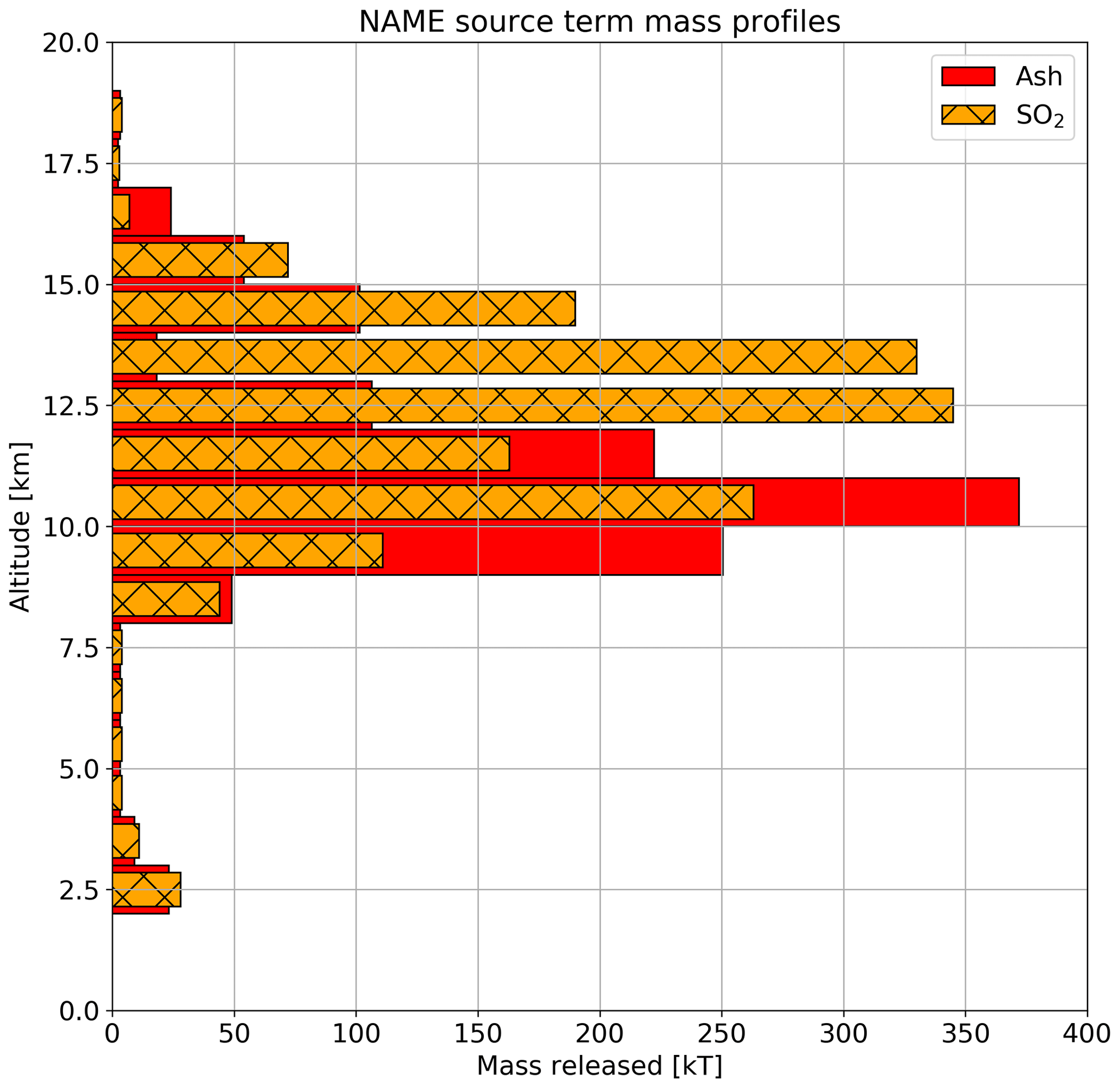
Figure 2 Height profiles of mass of ash and SO₂ released in NAME dispersion simulations of Raikoke. The ash profile (in red) was taken from the VolRes group report which used IASI satellite observations to arrive at an emission profile for SO₂. In lieu of a profile for ash only this profile has been adopted for the ash simulations. Plotted in orange (and hatched) is the StratProfile from Part 1 (de Leeuw et al., 2021) – this is the altered profile for the release of SO₂ arrived at following a detailed comparison between the SO₂ product from TROPOMI and NAME simulations. In this emission profile a larger fraction of the total mass of SO₂ is released in the stratosphere than in the original VolRes profile.

3.2.2 Sulfate aerosols

The sulfate aerosol results presented below are the result of the conversion of the simulated SO₂ into sulfate by the chemistry scheme within NAME, and no primary sulfur was emitted in the Raikoke simulation source term.

3.2.3 Volcanic ash

For volcanic ash simulations, the approach used by the London VAAC is to assume that most of the material ejected by an eruption is deposited close to the volcano, leaving only a fine mass fraction (FMF) available to be dispersed. Operationally this FMF is typically set somewhere between 1 % and 5 % of the total ejected mass, with 95 % to 99 % of the total mass assumed to have fallen out close enough to the volcano so as to have no influence on the subsequent observations/simulations. To estimate the amount of ash ejected during the 2019 Raikoke eruption, we have used the relationship between plume top height and mass eruption rate presented in Mastin et al. (2009). Using the plume top height of 15 km as reported by VolRes and eruption start and end times of 21:00 (UTC) on 21 June to 03:00 (UTC) on 22 June (taken from Himawari-8 imagery), we estimated a total ejected amount of ash of around 300 Tg. We use this estimate as a representative figure. We note that the eruption was not continuous during this time but rather progressed in several pulsed phases, each of which possibly reached different altitudes – and as such, this is an upper estimate. Using this value gives a FMF of between 3 and 15 Tg. Again taking the upper limit, we released a total of 15 Tg of ash over a vertical profile reported by the VolRes group (Fig. 2 in red). This vertical profile was formulated from a best estimate for the Raikoke SO₂ emission profile using Infrared Atmospheric Sounding Interferometer (IASI) measurements. In lieu of a specific profile for ash, we have adopted this SO₂ vertical profile as the best available estimate for ash. Note however that ash is not necessarily released in the same profile as the gas emissions.

3.2.4 Biomass burning aerosol

The location and vertical profile for the source term used to initialise the BBA dispersion simulation was derived from a MODIS image from the 17 June 2019 (shown in Fig. 1a). In this image a smoke cloud has already been advected in a north-easterly direction from an area of active forest fires. While there are no measurements available to show the height of the aerosol cloud, we assume that it is a hot and buoyant aerosol cloud that has continued to rise into the lower stratosphere as it was advected away from the source fires (Fromm et al., 2005, 2006). To represent this in NAME we have used a series of stacked and offset cylinders. A conceptual diagram of this structure is shown in Fig. 1b. An arbitrary mass of 0.1 Tg of material was released uniformly throughout each of the cylinders, on 100 000 particles, and the results later scaled to match observations (see Sect. 4). Panel (c) of Fig. 1 shows the concentration of model particles within each cylinder. The size and position of the cylinders was based only on the MODIS image shown in panel (a) of Fig. 1.

3.3 NAME output

Having initialised the simulations as described, NAME was configured to provide output files for (a) column loading (two dimensional – latitude × longitude) and (b) air concentration (three dimensional – latitude × longitude × altitude – with altitude measured from sea level). The data in each hourly file represent the mean of the simulated values calculated at 10 min intervals in the preceding hour.

3.4 Observations

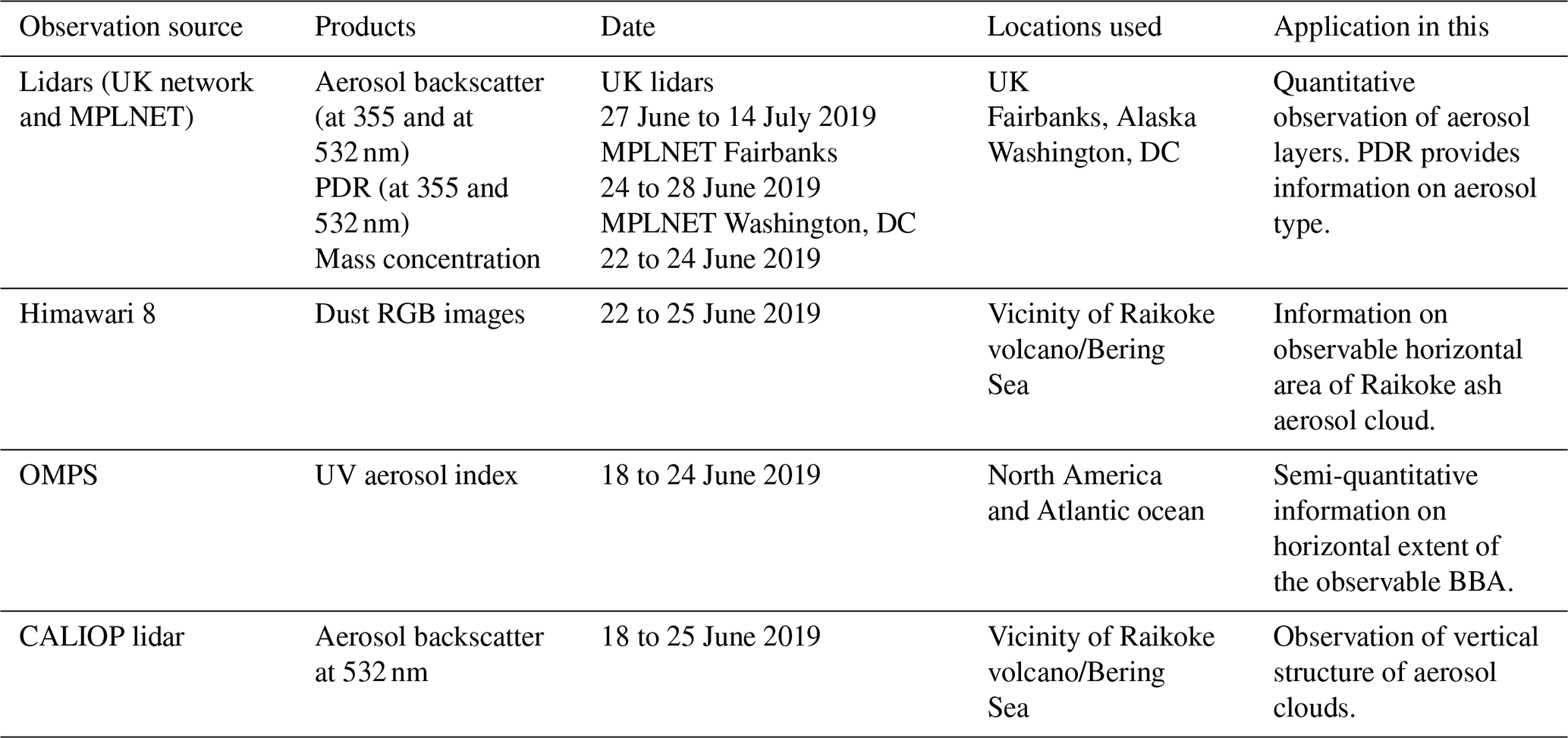
In this section we briefly describe the observations used to track the various aerosol clouds. The observations, platforms and applications in this study are summarised in Table 2.

Table 2 Summary of observations.

3.4.1 Surface-based remote sensing

UK lidars

The Met Office VA lidar network consists of nine fixed locations and one mobile facility (Osborne et al., 2019). Data recorded by three of the network lidars, Camborne, Loftus and Glasgow, are presented here. The instruments emit at 355 nm and have polar and co-polar depolarisation detection channels at 355 nm and an N₂ Raman detection channel at 387 nm. Aerosol optical properties are calculated from lidar analogue and photon-counting signals using a data analysis package developed at the Met Office which has been verified against the EARLINET Single Calculus Chain (SCC) (D'Amico et al., 2016; Mattis et al., 2016). Errors are estimated using the Monte Carlo method described in D'Amico et al. (2016). In Sect. 4 we use the particle linear depolarisation ratios (PDRs) measured by the lidars to assist with making aerosol identifications. Each lidar is calibrated using the ±45^∘ procedure from Freudenthaler et al. (2009). Additionally, we use the procedure described in Freudenthaler (2016) to correct for the polarisation effects of the various optical elements in the lidar. For each lidar we have also measured the angular offset between the plane of polarisation of the emitted laser beam and that of the optical elements used to split the incoming light by polarisation state, using a method similar to that described in Alvarez et al. (2006), and any measured offset has been included in the polarisation corrections. To confirm the robustness of the calibration, the volume depolarisation ratio is measured in pristine air and compared against a theoretical value calculated as in Behrendt and Nakamura (2002) and checked to see that it is within 1 % of expected values.

NASA-MPLNET lidars

The NASA Micro-Pulse Lidar (MPLNET) network currently has 17 active sites around the globe, each with a depolarisation MPL and a co-located Cimel sun photometer (Welton et al., 2001; Welton and Campbell, 2002; Welton et al., 2018). The instruments operate at 532 nm and also have co-polar and cross-polar depolarisation detection. To study the vertical structure of the Raikoke and BBA clouds we make use of data from the MPLNET sites at Fairbanks in Alaska (64.86^∘ N, 147.85^∘ W) and the Goddard Space Flight Center in Washington, DC (38.99^∘ N, 76.84^∘ W). We make use of the products from the new version 3 processing system, which provides the normalised relative backscatter (NRB), volume depolarisation ratio (VDR) and particle linear depolarisation ratio. The data are available for download from https://mplnet.gsfc.nasa.gov/ (last access: 16 July 2020).

Ansmann et al. (2011)Marenco et al. (2011)Thomason and Peter (2006)(Palmer and Williams, 1975)(Thomason and Peter, 2006)Petzold et al. (2007)(Bluvshtein et al., 2017)(Bluvshtein et al., 2017)

Table 3 Aerosol specific extinction values and assumed refractive indices (R.I.) and densities (ρ).

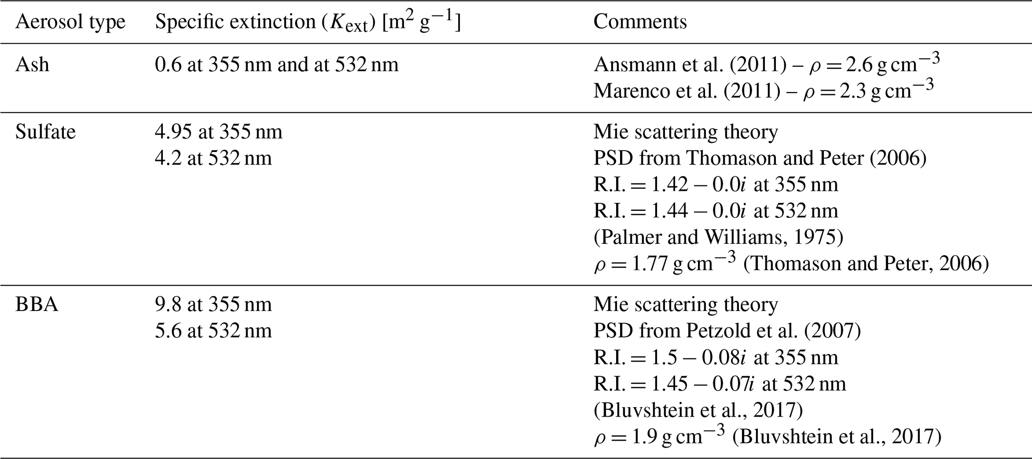
Using data from UK and MPLNET lidars we have derived aerosol mass concentration estimates using the aerosol specific extinction values (K_ext) listed in Table 3 to convert extinction profiles to mass estimates. For sulfate and BBA aerosols we have used literature values for refractive index and stratospheric size distributions in Mie scattering calculations, along with literature values for density, to calculate a representative K_ext. In the case of irregularly shaped volcanic ash particles, for which Mie calculations are unsuitable, we have used a literature value. We do not take into account factors such as hygroscopic growth or particle cohesion that will have an effect on scattering efficiency, and these values are representative only. A more complex treatment of K_ext is beyond the scope of this study. Errors in both the lidar extinction and backscatter retrievals as well as the calculation of K_ext contribute to the uncertainties in the final mass estimates. As stated above, errors in the lidar retrievals have been calculated using a Monte Carlo technique (D'Amico et al., 2016), taking into account both the statistical errors in the raw lidar signals and errors in the systematic parameters used in the processing, such as assumed lidar ratios and polarisation factors. Again following the methods of Ansmann et al. (2011) the uncertainty on K_ext has been estimated by propagating the error in the assumed aerosol densities and the variation in the sun-photometer-derived factors. In total, the error in the mass estimates is on the order of ± 50 %.

Dust RGB images

In Sect. 4 we present dust RGB images made using infrared bands B11 (8.6 µm), B13 (10.4 µm) and B15 (12.4 µm) from the advanced Himawari imager carried by the Himawari-8 satellite and compare these with the NAME model simulations for volcanic ash (Francis et al., 2012). The RGB images were created by assigning red to the difference between B15 and B13, green to the difference between B13 and B11, and blue to B13. In this scheme, aerosol clouds containing volcanic ash should appear bright red, or bright yellow if there is also significant SO₂ (Francis et al., 2012). While not a quantitative measure, the RGB imagery is useful for assessing the horizontal spatial distribution of volcanic ash clouds during the initial dispersion.

UV aerosol index

The Ozone Mapping and Profiler Suite (OMPS) carried in the Suomi NPP satellite measures backscattered ultraviolet radiance. The UV aerosol index (AI) is derived from radiances at 340 and 378.5 nm, with a temporal resolution of 24 h (Torres et al., 1998, 2018). A positive AI value indicates the presence of UV absorbing aerosols such as dust (Christopher et al., 2008), volcanic ash (Carn and Krotkov, 2016) or smoke (Torres et al., 2020). The parameter is unitless and takes a value between 0.0 and 5.0, with 5.0 indicating heavy aerosol loads. The AI is available from https://snpp-omps.gesdisc.eosdis.nasa.gov/data/SNPP_OMPS_Level2 (last access: 21 June 2020). The product is semi-quantitative and is used in Sect. 4 to assess the horizontal spatial distribution of the BBA cloud from the Alberta fires.

CALIOP backscatter and aerosol vertical feature mask

The Cloud-Aerosol Lidar with Orthogonal Polarization (CALIOP) lidar on board the CALIPSO satellite measures elastic backscatter and depolarisation at 532 and 1064 nm (Winker et al., 2009). The level 2 data downloaded, available from http://www-calipso.larc.nasa.gov (last access: 10 July 2020), also include a vertical feature mask (VFM), which identifies aerosol layers and assigns an aerosol subtype – for example dust, volcanic ash or elevated smoke (Omar et al., 2009). In Sect. 4 we use CALIPSO data to assist with tracking both the volcanic and BBA aerosol clouds as they travel to the UK.

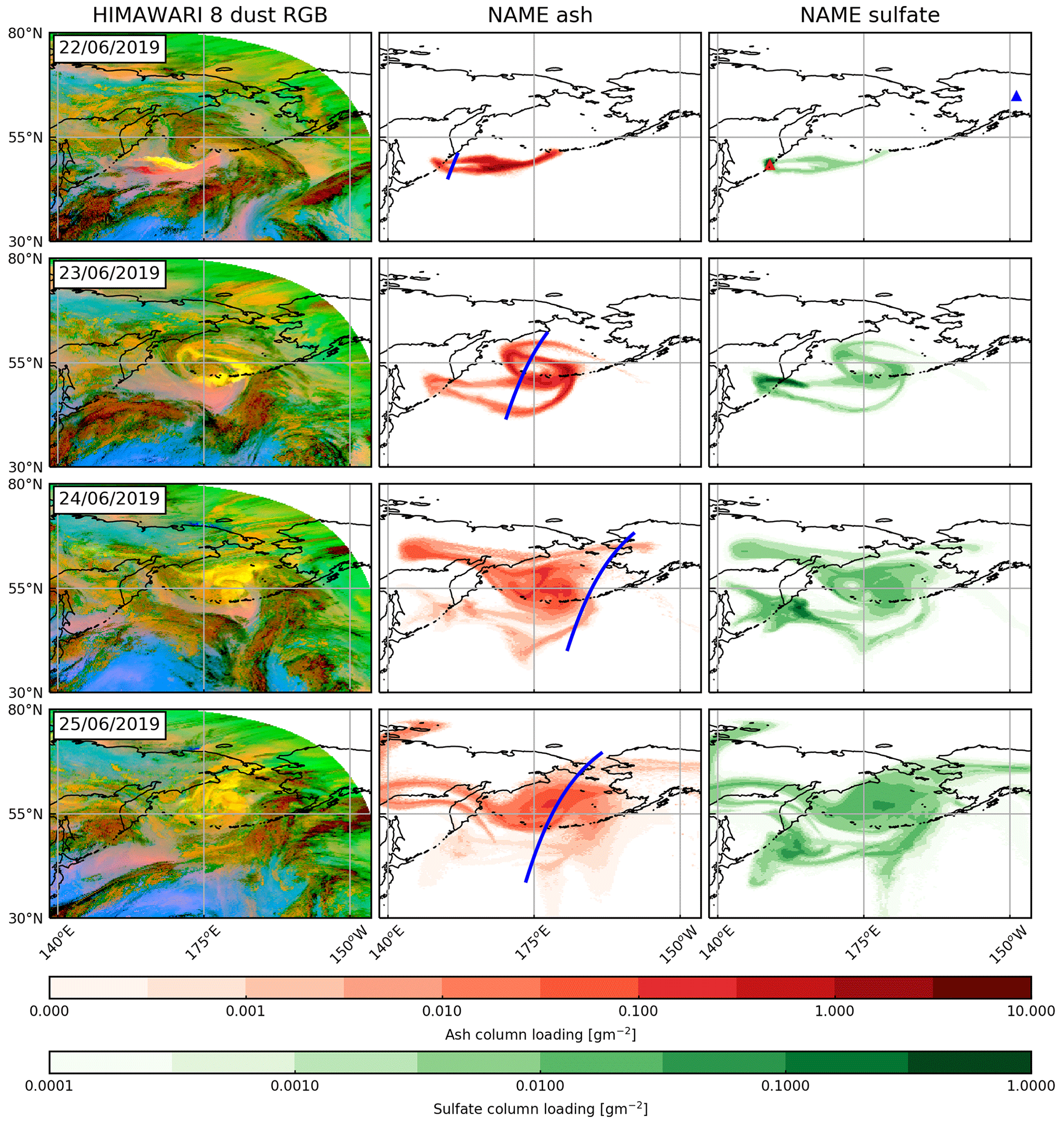
Figure 3 Column one: Himawari-8 dust RGB for dates shown; columns two and three: NAME simulated column loadings for ash and sulfate clouds [g m⁻²]. Both the Himawari data and the NAME simulation data are for 15:00 UTC on the date shown. The red and blue triangles in the upper-right panel show the locations of the Raikoke volcano and the Fairbanks MPLNET lidar respectively. The blue line in the central column shows the CALIPSO track at that time.

3.4.2 IAGOS aircraft-based observations

The European research infrastructure In-service Aircraft for a Global Observing System (IAGOS; see https://www.iagos.org, last access: 12 February 2021, for details) performs routine measurements of basic atmospheric state variables, atmospheric chemistry and aerosols using their standard payload on a fleet of passenger aircraft equipped with IAGOS-CORE instruments (Petzold et al., 2015). In addition to the standard equipment, a single Lufthansa Airbus 340–600 carries the more sophisticated IAGOS-CARIBIC (Civil Aircraft for the Regular Investigation of the atmosphere Based on an Instrument Container) instrumentation (Brenninkmeijer et al., 2007). During the time period of our investigation, the IAGOS-CARIBIC aircraft made several chance penetrations of the BBA cloud originating from Alberta, making measurements with the IAGOS aerosol instrument (Bundke et al., 2015), which contains an optical particle counter (OPC; Grimm model 1.129 Sky) and a set of condensation particle counters (GRIMM model 5.411). The optical particle counter used here measures particle concentration (as number of particles per cubic centimetres) for particle diameters between 0.25 and 2.5 µm.

4 Results and discussion

In this section we use the NAME simulations and the various observational data to chart the course of the aerosol clouds produced by the Raikoke eruption and the Alberta forest fires as they were transported to the UK, before using the simulations to assist in interpreting the UK lidar data. We first look at the initial 5 to 6 d subsequent to the emission of the ash and BBA and then use the NAME simulations to track the transport to the UK.

4.1 Volcanic aerosols: transport

The left-hand column of Fig. 3 shows the Himawari-8 dust RGB images for the first 4 d after the 21 June Raikoke eruption. The central column shows the NAME simulated column loadings for volcanic ash, and the right-hand column shows the NAME simulated column loadings for sulfate aerosol. In the simulations both the ash and sulfate aerosol clouds initially move east from the volcano while also dispersing to the north and south. The leading edges of the aerosol clouds then begin to be entrained by a low-pressure cyclonic system centred at around 55^∘ N and 175^∘ W (seen as a green and brownish cloud in the RGB image) and turn northwards over the Aleutian Islands.

The eastern ends of both the ash and sulfate clouds split into two distinct structures, corresponding to the red and yellow areas in the RGB image. The simulated aerosol clouds continue to disperse and reach Russia by 24 June and Alaska by 25 June. As expected, the sulfate aerosol concentration is initially relatively low and increases as the oxidation of SO₂ progresses. The RGB images reflect the general structure of the most intense parts of the model-simulated aerosol clouds and show the aerosol cloud moving east and being entrained in the warm conveyor of the cyclonic system before encircling it and dispersing to the east and west. Figure 3 shows that on 22 June the northern part of the aerosol cloud is bright yellow – indicating the presence of SO₂ as well as ash, whereas the south-westerly part is bright red, indicating that the infrared emission in this region was dominated by ash (Francis et al., 2012). Several of the model structures are absent, however, and this may in part be due to an overlying cloud obscuring the aerosol cloud from the sensor. For example, on 23 June the most southerly structures in the model aerosol clouds are co-located with an area of cloud in the RGB images, which appear as green and brownish colours. After 25 June the aerosol cloud can no longer be discerned in the RGB product.

4.2 Volcanic aerosols: vertical structure

Figure 4 shows the model ash and sulfate aerosol cloud air concentrations along the CALIPSO tracks shown in Fig. 3, alongside the CALIPSO attenuated backscatter at 532 nm and the VFM. On 22 June the CALIPSO track passes over the separated part of the aerosol cloud that is shown on both the RGB observation and the simulations. The northern part is shown by CALIPSO at around 17 km (49^∘ N latitude) and has been classified as volcanic ash in the CALIPSO VFM (9: light grey), and the southern part is found to be lower at under 5 km. This lower part is identified in the VFM as mineral dust (2: yellow). Kim et al. (2018) explain that only aerosols in the stratosphere can be identified as volcanic ash or sulfur by the VFM. Below the tropopause volcanic ash will often be classified as dust or polluted dust and volcanic sulfate will often be classified as elevated smoke. This could explain the way these two plumes are captured in the CALIPSO VFM. Note that as seen in the dust RGB, both the northern (stratospheric) plume and the southern (tropospheric) plume are too weak to be identified in the dust RGB at the location of the CALIPSO overpass; however, both plumes become more intense further east, and the difference in colour in the dust RGB is indicative of a strong signal from SO₂ in the northern aerosol cloud.

On 23 June the effect of the cyclonic system is evident with the two vertical structures at around 52 and 56^∘ N, indicating the walls of this central pressure low. The tops of these structures are visible in the CALIPSO attenuated backscatter data. The structure at around 43^∘ N below 5 km and identified as dust in the VFM is not visible in the RGB image, possibly because it is occluded by the cloud at around 10 km. In areas where the model places ash in the troposphere, the VFM has identified this as dust or polluted dust (2: yellow; 5: brown), and sulfate has sometimes been identified as elevated smoke (6: black). Almost all of the stratospheric layers identified in the VFM have been given the “volcanic ash” classification (9: light grey), with very few “sulfur/other” classifications. According to Kim et al. (2018) the distinction between the two classifications for layers that are optically thicker than 0.001 sr⁻¹ (vertically integrated attenuated backscatter) is based on the PDR: if it is above 15 % the layer will be classified as volcanic ash. Depending on the relative concentrations, a mixture of sulfate aerosols (PDR ≈ 1 %; e.g. Ansmann et al., 2012) and strongly depolarising volcanic ash (PDR ≈ 35 %; e.g. Ansmann et al., 2011) may well result in an overall PDR of more than 15 % (Groß et al., 2013) – and the designation of these layers as ash in the VFM is not inconsistent with an ash-rich mix of ash and sulfate aerosols.

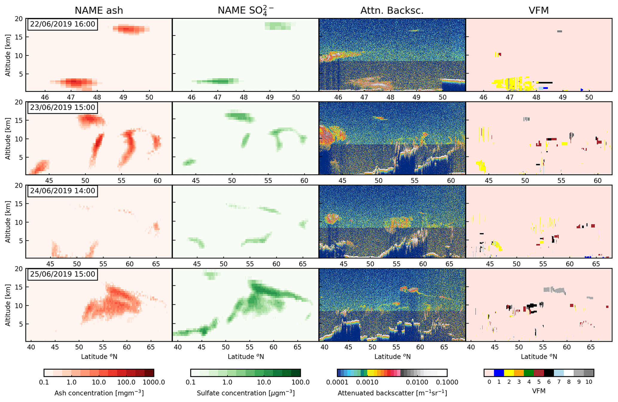
Figure 4 Columns one and two: vertical distribution of simulated ash and sulfate aerosol clouds along the CALIPSO tracks shown in Fig. 3; column three: CALIPSO total attenuated backscatter at 532 nm; column four: CALIPSO VFM. The model data are taken from the 1 h output file closest to the time of the CALIPSO overpass. Key to VFM colour bar: 0 means not applicable, 1 means marine, 2 means dust, 3 means polluted continental/smoke, 4 means clean continental, 5 means polluted dust, 6 means elevated smoke, 7 means dusty marine, 8 means polar stratospheric cloud aerosol, 9 means volcanic ash and 10 means sulfate/other.

After having analysed the volcanic plume dispersion over the ocean using CALIPSO, we can keep following the ash and the sulfur aerosol over the American continent from ground-based remote-sensing instruments. Figure 5a shows the attenuated backscatter data from the NASA-MPLNET lidar in Fairbanks, Alaska (64.86^∘ N, 147.85^∘ E), from 24 to the 28 June 2019. Late on 24 June a banked structure (red outline 1) can be seen starting at 10 km and descending to around 5 km by 26 June. While this structure is mostly dominated by meteorological cloud, it appears to contain some aerosol, noticeable in the areas with no cloud. The data do not allow the retrieval of a PDR or mass concentration in this structure. Above this structure (red outline 2) a vertically thin aerosol layer can be seen at around 12 km, persisting from early on 25 June until around midday on 27 June. The whole day mean PDR within this layer on 26 June is 25 %, consistent with a mixture of ash and sulfate particles (Ansmann et al., 2011; Groß et al., 2013). Using assumed values for PDR for ash (35 %) and sulfate (1 %) together with an ash-like specific extinction of 0.6 m⁻² g⁻¹ (Ansmann et al., 2011; Marenco et al., 2011) and a Mie-calculated sulfate specific extinction of 4.2 m⁻² g⁻¹ to convert the particle extinction measurements into separate mass concentration estimates for ash and sulfate, the mean estimates within this layer are 250 and 10 µg m⁻³ for ash and sulfate respectively. Given the uncertainty of the assumptions for PDR and specific extinction, the error on these mass estimates is on the order of 50 % (Ansmann et al., 2011; Osborne et al., 2019). A second banked structure (red outline 3) starts at 11 km at midnight on 26 June and descends to the boundary layer top by mid-afternoon on 27 June. While mostly obscured by low tropospheric clouds at around 2.5 km, there are indications of aerosol layers observable in this structure. Again, the sparse data do not allow the retrieval of either a PDR or mass concentration within this structure.

Panels (b) and (c) in Fig. 5 show the NAME simulated air concentrations for ash and sulfur respectively. The outlined regions from panel (a) are also marked in panel (b) with dashed lines for reference. The structure of the two simulated aerosol clouds are similar to each other, with an initial sloping structure starting at around 10 km on 25 June, descending to 4 km by midday on 27 June, and a geometrically thin layer at 11 to 13 km. Such sloping lidar features are frequently observed owing to vertical shear in the atmosphere with faster transport at higher altitudes (e.g. Dacre et al., 2015). Both of these structures are somewhat representative of the outlined structures 1 and 2 in the lidar data. However, there is a large structure between 5 and 10 km in the simulations that is not present in the lidar observations. Attempts at modifying the vertical structure of the ash source term by changing the mass released at each altitude could not remove this structure. A thorough investigation of the cause of this discrepancy is beyond the scope of this study, but we note that this is a significant difference between the simulations and lidar observations.

The maximum concentrations in the higher layers between the times indicated by the vertical red lines are 400 and 25 µg m⁻³ for the ash and sulfate simulations respectively. While these values are higher than those estimated from the lidar data, they are of the same order of magnitude (and their ratio is more or less the same), giving some indication that the fine mass fraction of ash is allowed to remain in the simulations, and the amount of sulfate produced in the simulations by the chemistry scheme is somewhat representative of the real values.

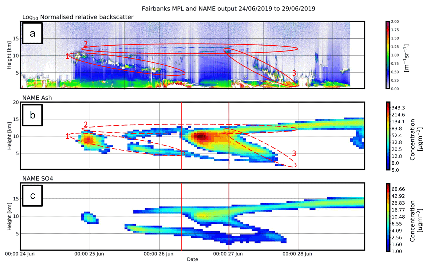
Figure 5 Fairbanks MPL lidar: (a) normalised relative backscatter [m⁻¹ sr⁻¹]; (b, c) NAME simulated air concentrations for ash and sulfate respectively [µg m⁻³]. Data for 24 to 28 June 2019. The red outlines labelled 1, 2, and 3 and the vertical red lines are discussed in the text.

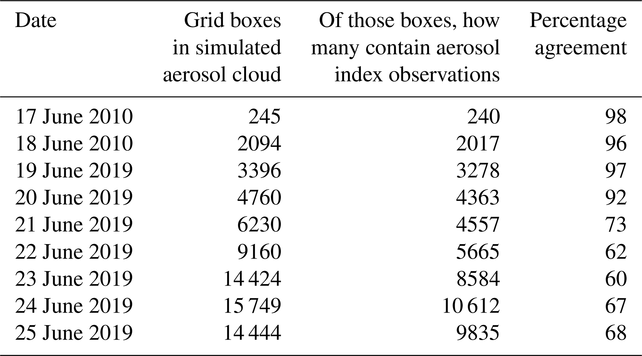
Table 4 Comparison between OMPS AI and NAME BBA simulation. Each simulated grid box is 0.2^∘ latitude × 0.4^∘ longitude at the surface – approximately 20 km × 40 km at mid-latitudes.

4.3 Biomass burning aerosol: transport

Figure 6 shows the OMPS AI, together with the NAME simulated BBA column loadings for 18 to 24 June. In both the simulations and the AI the BBA cloud initially moves fairly uniformly north-east towards Hudson Bay for around 24 h, before the leading edge is caught in an anticyclonic system and part of it begins to turn south before looping back and turning north and then east once again by 19 June. On 20 June the easterly edge of the aerosol cloud has crossed Hudson Bay and, in both the measurements and the simulation, the BBA aerosol cloud is also starting to extend westwards towards the Pacific coast. By 21 June the north-eastern edge of the aerosol cloud has reached the Labrador coast, while the southern edge has been caught in a north-westerly jet and is moving across the continental United States towards Washington, DC. The western extent of the model aerosol cloud is now reaching to the Pacific coast, but this is not the case in the AI, and this part of the simulated aerosol cloud is absent from the measurements. By 22 June the leading edge of the southerly aerosol cloud has moved beyond Washington, DC, and out over the Atlantic where it has been entrained in a cyclonic system centred off the coast of Newfoundland and turned northwards. The more northerly part of the aerosol cloud is moving towards Greenland and over Iceland by the 23 June. By 24 June, this more northerly part has now turned south and moved over the Atlantic towards the west of Ireland. The southerly part of the aerosol cloud has continued to be entrained by the cyclonic system and has itself moved north to Greenland. Missing entirely from the AI is the large structure that extends out to the Pacific coast. This feature is also not present in any CALIPSO profiles. This part of the simulated aerosol cloud originated almost entirely from material released at the very top of the model source, between 16 and 18 km, and this suggests therefore that the BBA cloud did not extend above 16 km. In terms of spatial extent and horizontal structure, many of the features of the simulated BBA cloud are reflected in the AI, particularly in the first 3 to 4 d. However, the simulated aerosol cloud looks to be more diffuse than is suggested by the AI observations. This may in part be due to the detection limits of the AI, which is unlikely to be sensitive to some of the very low column loadings suggested by the model simulations. For example, as is shown in Sect. 4.4, CALIPSO lidar soundings along the tracks marked in panels (j), (l) and (n) of Fig. 6 detect elevated smoke in regions without significant AI index values (see panels i, k and m of Fig. 6), showing that the BBA cloud can be present even where no AI index is observed. A quantitative comparison between the AI index and NAME simulations is difficult not only because the lower concentrations can be missed by the AI index, but also because the AI index is sensitive to other common aerosols (for example dust – see Met Office operational dust forecast plotted in Fig. 6), and so will always detect significant amounts of background aerosol. However, to give some quantification within the bounds of the simulated BBA cloud we have re-gridded the AI onto the same latitude–longitude grid as the NAME simulations and compared the number of grid boxes within the simulated aerosol cloud that also have a positive AI index. The results of this comparison are shown in Table 4. For the first 4 d following emission over 90 % of the grid boxes within the simulated BBA cloud also contain an AI observation. This then falls to as low as 60 % over the next 4 d.

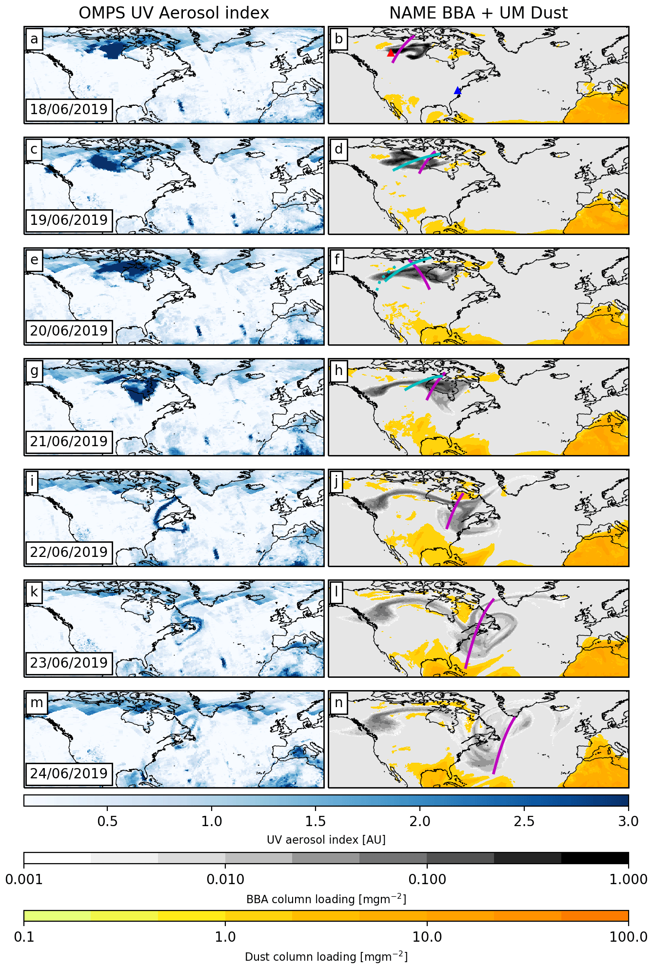
Figure 6 Left-hand column: daily composites of OMPS UV aerosol index. Right-hand column: simulated column loadings for BBA (black – mg m⁻²) and UM dust column loadings (yellow – mg m⁻²) for 12:00 UTC on the date shown. The source location for simulated BBA particles is shown in the uppermost right-hand panel as a red triangle, and the location of the Washington MPL lidar station is shown as a blue triangle. In the right-hand panels a selection of CALIPSO overpasses are marked in magenta, and four CARIBIC flight tracks are marked in cyan.

While there have been efforts to determine the relationship between aerosol index and aerosol optical depth and hence column loading, such relationships are frequently spatially variable owing to the sensitivity of the aerosol index to both the aerosol absorption optical depth and the altitude of the aerosol cloud (e.g. Christopher et al., 2008). BBA in the stratosphere will likely be associated with a stronger AI than a similar column loading of BBA in the troposphere. A more quantitative assessment of the aerosol column loading utilising the AI is beyond the scope of this paper.

4.4 BBA: vertical structure

Figure 7 shows the vertical structure of the simulated and observed BBA cloud along the CALIPSO tracks shown in Fig. 6. The timings of the NAME simulations match the CALIPSO overpass times and so are shifted in time by a few hours compared to that shown in Fig. 6; the timing of the model data is shown in each panel in the left-hand column. The comparison between the model data and the CALIPSO sounding on 18 June is poor, with no features in the model matching the height or location of features in the measurements. In particular, the large feature between 16 and 18 km in the model data is entirely absent from the CALIPSO sounding. This feature corresponds to the model particles released above 16 km, and as stated above, it seems likely that the aerosol cloud did not initially reach above this height. Also missing is the large area identified as elevated smoke in the VFM (black) in the boundary layer between 57 and 62^∘ N. Given the relatively small scale of the BBA cloud smoke on this day compared to the more developed aerosol cloud over the following days, the comparison is sensitive to small offsets in time and space between the observations and the model output. However, shifting the model data by a few degrees did not improve the comparison. By 19 June the comparison is more favourable, with some features in the model data corresponding in height and location with features in the CALIPSO sounding that have been classified as elevated smoke in the VFM. While the structure in the model data at around 9 km between 57 and 60^∘ N is not present in the VFM, there is some indication of it in the attenuated backscatter, and it may be the case that the classification scheme has failed due to the signal being attenuated by the optically thick structure above. From 20 June onwards the comparison improves as the aerosol cloud disperses into a larger structure and continues to be shaped by the synoptic meteorology. By 22 June the structures in the CALIPSO soundings identified as elevated smoke or sulfate/other (dark grey) are all present in the model data, and by 23 and 24 June there is good agreement between the two in terms of structure and position.

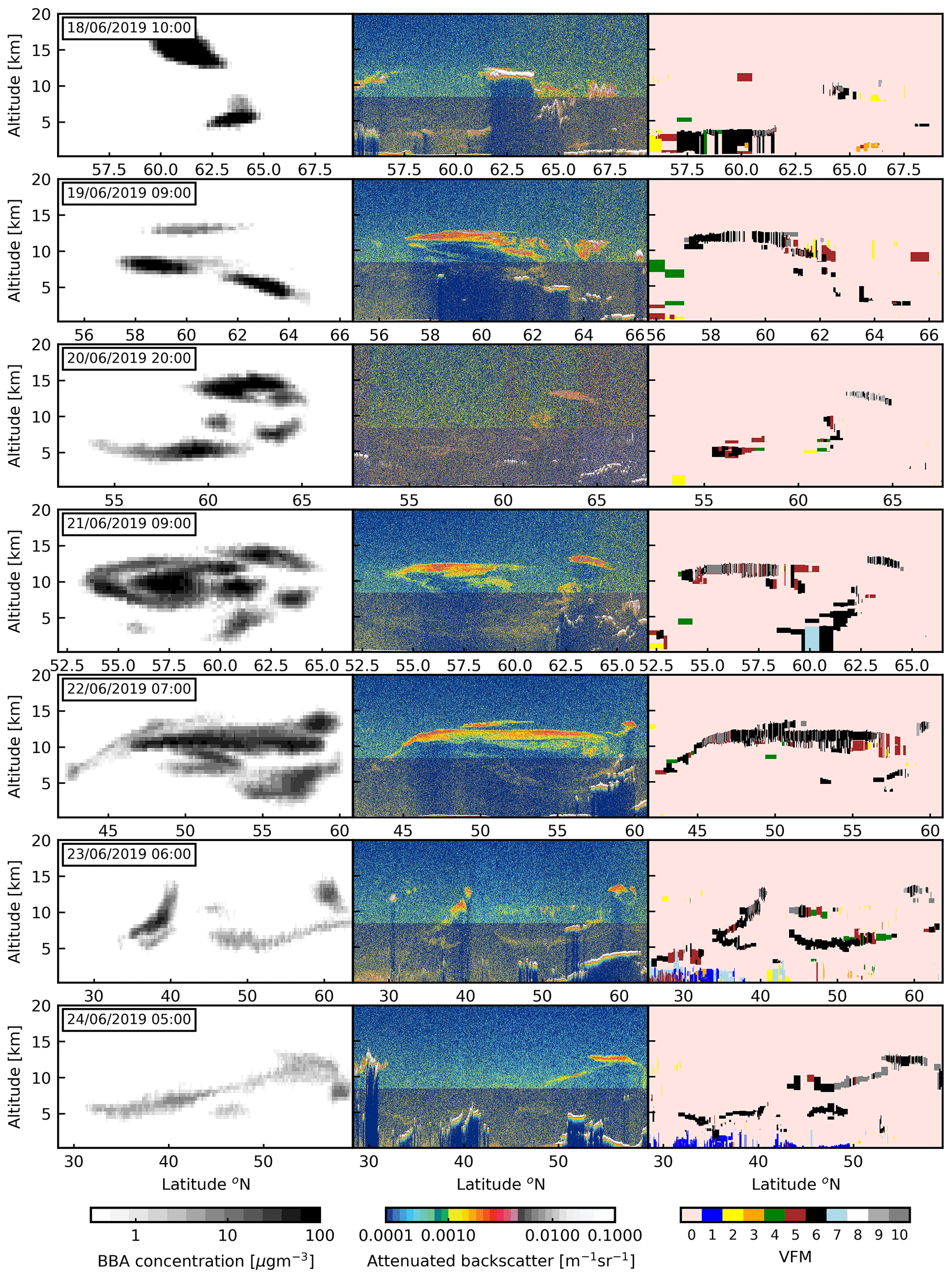
Figure 7 Left-hand column: vertical structure of the NAME BBA mass concentrations along the CALIPSO tracks shown in Fig. 6 [mg m⁻³]; middle column: CALIPSO total attenuated backscatter at 532 nm [m⁻¹ sr⁻¹]; right-hand column: CALIPSO vertical feature mask. The NAME data are taken from the output file closest to the time of the CALIPSO overpass and so are shifted in time slightly compared to that shown in Fig. 6. Key to VFM colour bar: 0 means not applicable, 1 means marine, 2 means dust, 3 means polluted continental/smoke, 4 means clean continental, 5 means polluted dust, 6 means elevated smoke, 7 means dusty marine, 8 means polar stratospheric cloud aerosol, 9 means volcanic ash and 10 means sulfate/other.

Figure 8a shows the relative attenuated backscatter product from the Washington MPLNET lidar between 00:00 on 22 June and 23:59 UTC on 24 June. Panel (c) shows the NAME BBA concentration for the grid box over Washington, DC, for the same time. Although it is initially partly obscured by clouds, a well-defined aerosol layer arrives over the site at around midday on 22 June. Beginning as a single layer at an altitude of 5 km, the layer then rises slightly to 8 km, before descending to around 4 km and splitting into upper and lower layers, separated by around 500 m, by mid-morning on 23 June. The layers then persist until midnight on 23 June. The mean PDR with these layers (at 532 nm) is 8±2 %, consistent with the layer being composed of BBA (Groß et al., 2015a; Adam et al., 2020). Using a specific extinction value of 5.6 m² g⁻¹ (calculated using Mie scattering theory) and assuming a refractive index of 1.5−0.07i at 532 nm, a density of 1.9 g cm⁻³ and a size distribution taken from (Petzold et al., 2007) to transform the extinction coefficient product to a mass concentration estimate, the mean backscatter weighted concentration within the layers is 15±5 µg m⁻³.

The general shape and position of this aerosol layer is also represented in the simulations, with good agreement for altitudes and timing. The size of the separated structure shown in the lidar data is on the order of the 500 m altitude grid on which the NAME data are reported, and it is therefore unsurprising that this has not been resolved by the model. By scaling the amount of mass released in the Alberta fires source term, it is possible to match the model concentrations above the Washington, DC, site to the lidar concentration estimates. Scaling the altitude bins uniformly from the ground to 16 km results in 0.2 Tg of particulate material being released in the model.

Figure 8 Washington MPL lidar data: (a) normalised relative backscatter [m⁻¹ sr⁻¹]; (b) volume depolarisation ratio [%]; (c) NAME air concentrations for BBA cloud [µg m⁻³]. The NAME data have been scaled to match the lidar concentrations estimates. Data for 22 to 24 June 2019.

4.5 BBA regional analysis over North America

Figure 9 shows the NAME simulated mass concentrations of BBA along the IAGOS-CARIBIC flight tracks marked in Fig. 6. Overlaid on the model data are the flight paths colour coded to show the particle numbers (per cm³ of air) counted by the Grimm OPC on board the IAGOS-CARIBIC aircraft. For flight F570 on 19 June and during flight F571 on 20 June there is remarkable agreement between the locations in which the aircraft encountered elevated particle numbers and the location of the simulated aerosol cloud. This is particularly true of flight F571, where the particle counts indicate where the aircraft has encountered an initial region of elevated particle counts at 10 km, centred on 62^∘ N, followed by a relatively particle-free region, and then a second region of elevated particle counts at around 67^∘ N, all of which agree well with the aerosol cloud locations in the model. Flight F572 has not encountered any areas of elevated particle counts. According to the model, it has flown under the large structure that extends out to pacific coast (see Fig. 6); however, as stated above, this structure does not appear in the OMPS or CALIPSO measurements and is likely a model artefact. Flight F573 has flown between two separated parts of the model aerosol cloud. On this occasion, the locations of the CALIPSO track and the flight track cross at around 63^∘ N (although the flight track is between 06:00 and 07:00 and the CALIPSO overpass at 08:44 UTC) and a similar separated structure can be seen in the CALIPSO soundings on 21 June at around 63^∘ N.

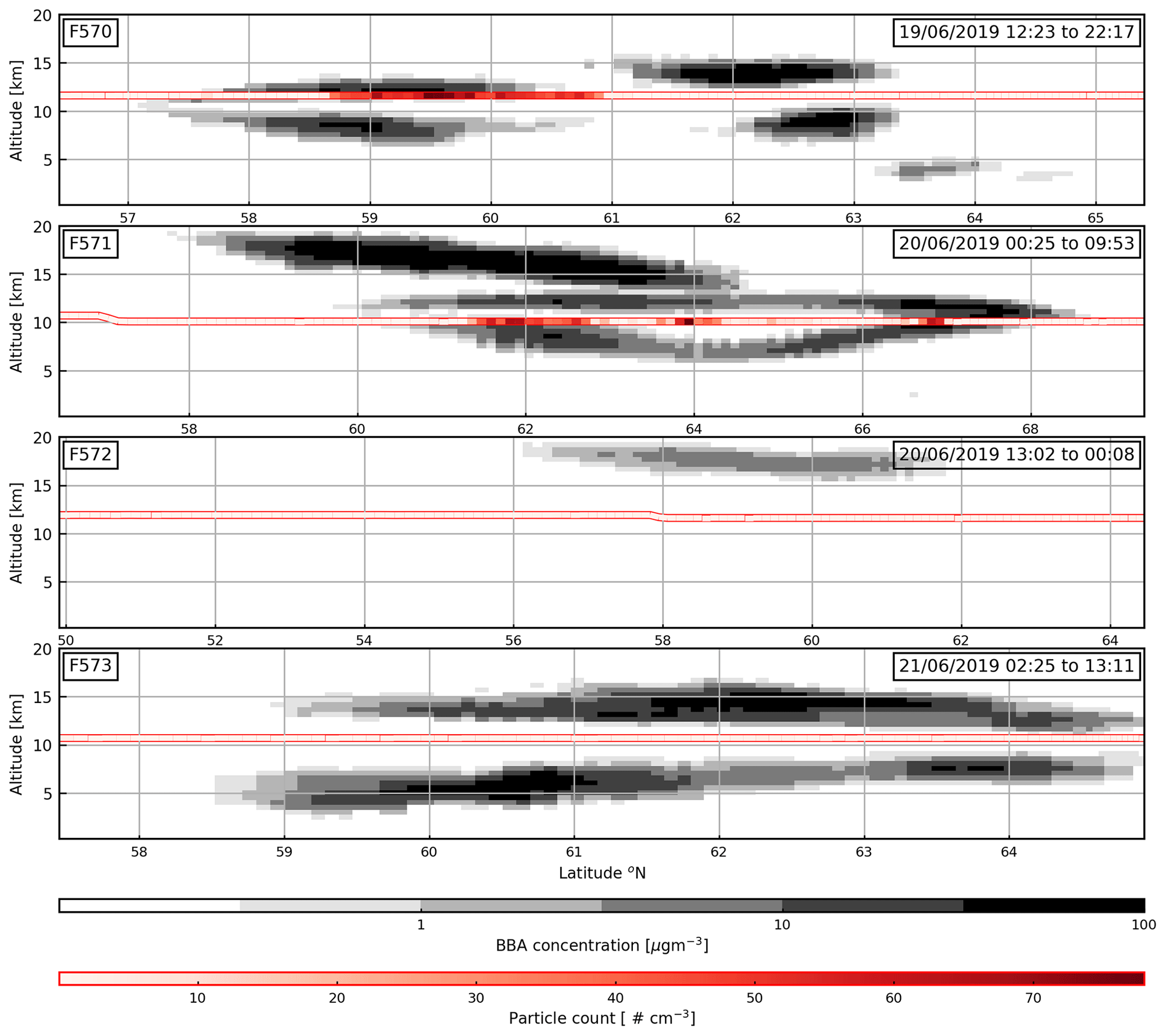
Figure 9 NAME air concentration data [µg m⁻³] along the CARIBIC tracks shown in Fig. 6. Overlaid are the CARIBIC flight paths coloured to show the particle count [number cm⁻³] recorded by the Grimm OPC. The NAME data are a mean of the 1 h output files corresponding to the time the aircraft was transiting the aerosol cloud (times shown in panels).

So far we have presented the observation data and NAME simulations together, charting the dispersion of the volcanic and BBA clouds over the first 5 to 6 d. The observations indicate that the NAME simulations reflect the general pattern of the dispersion seen in the various observations and as such can be used to gain some insight into the dispersion of the aerosol clouds in areas where there are no observations. The availability of observations as the aerosol clouds crossed the Atlantic towards the UK is sparse, as the concentrations were mostly below the detection limits of passive satellite observation, and so we now rely upon only the simulations as the aerosol clouds move towards the UK and mainland Europe. Figure 10 shows the column loadings for all three simulated aerosols on 27 June, 1 July and 11 July. The Met Office operational dust forecast is also plotted with the BBA column loadings. The NAME simulations show the BBA cloud having reached the UK by 27 June, along with an aerosol cloud of Saharan dust. The Saharan dust moves away from the UK over the next 4 d; however, the BBA cloud persists over the UK and is joined on 1 July by the ash aerosol cloud and the first parts of the sulfate aerosol cloud.

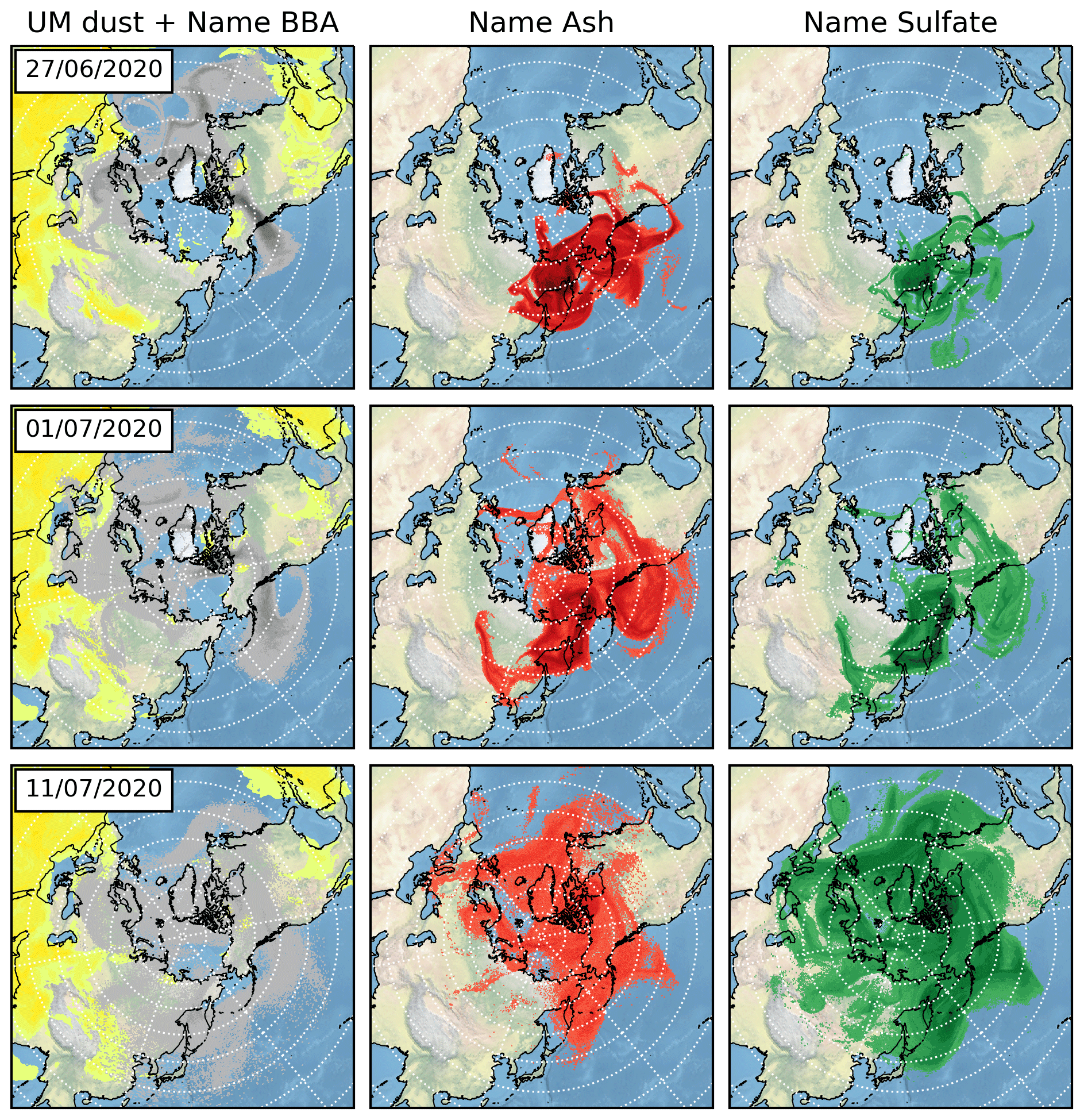
Figure 10 NAME dispersion model simulations for BBA (black/grey) (with UM dust field in yellow), ash (red) and sulfate (green). Data for 00:00 UTC on date indicated in each panel.

Both simulated aerosol clouds continue to impact the UK over the next week to 10 d, while also dispersing over much of the Northern Hemisphere. By 11 July the more substantial parts of the simulated sulfate cloud also reached the UK.

4.6 Regional analysis and interpretation of material over the UK

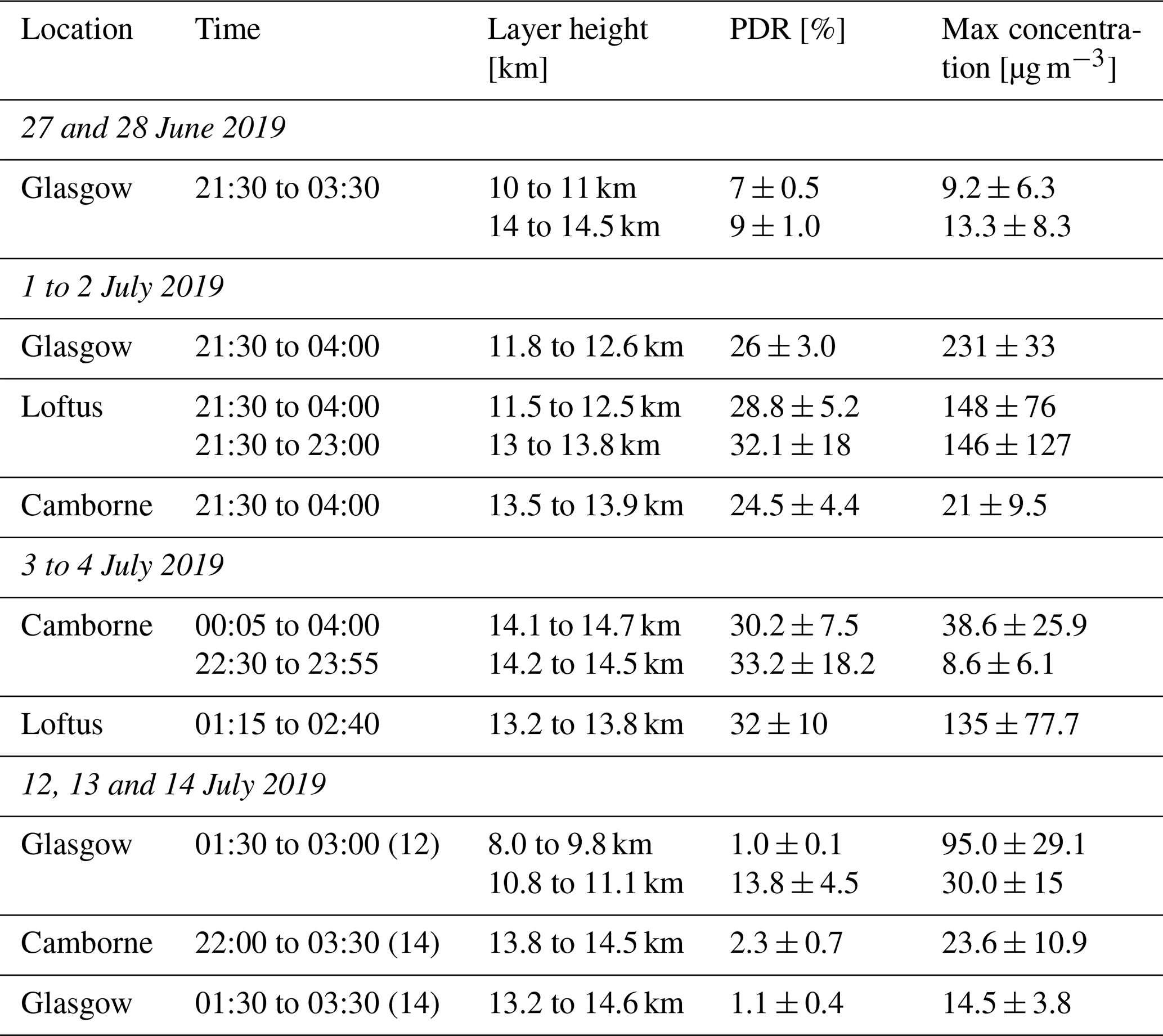
Figure 11 shows examples of the data from the network lidars recorded on the dates displayed in Fig. 10. Features discussed below are outlined in red and yellow. The upper axis in each panel shows the log10 of the range-corrected signal, and the lower axis shows the log10 of the volume depolarisation ratio. Table 5 gives a summary of the aerosol layers measured across the network. To be consistent with the simulations the heights quoted are above sea level. As described below we have used long averaging windows to calculate backscatter and PDR. However, even using this large averaging time it was not possible to measure the lidar ratio (which involves dividing a noisy signal by another noisy signal) as the results were so noisy as to be unusable.

The network first detected stratospheric layers over the Glasgow site on the evening of 27 June, with an upper layer at 14 km and a lower layer at 11 km (both outlined in red in panel a in Fig. 11). There is also a much thicker layer in the troposphere between 2 and 6 km after around 04:00 on 28 June (outlined in yellow). In this lower layer the mean PDR (at 355 nm) was 26±3 %. This is consistent with the layer being comprised of Saharan dust (Groß et al., 2013; Osborne et al., 2019), and the Met Office operational dust forecast confirms that this is the source of this lower altitude layer and that it is unrelated to either the forest fires or the Raikoke eruption. The measurements in the stratospheric layers are near the limit of the useful range of the lidars (≈ 15 km), and the layers were only detectable at night when the daylight background was absent. To calculate PDR values and mass estimates at this range we have used whole night averages (6 h of continuous photon counting) to improve the signal-to-noise ratio as far as possible. We note that this assumes that the aerosol particle type and properties remain constant during that time. Using the whole night average, as well as the Raman and elastic channels, we calculate that the PDR in the upper and lower layers was 9±1 % and 7±1 % respectively. There are a very limited number of reported measurements of the PDR of stratospheric BBA at 355 nm. Hu et al. (2019) report values of up to 26 %, and Haarig et al. (2018) report values around 20 %. These values are considerably higher than our measurement. It is possible that the variation is due to differences in the production and ageing process of the aerosols in this layer compared to those measured in the previous studies. Tropospheric measurements of PDR of BBA are much more numerous and are often reported to be below 5 % (e.g. Groß et al., 2015b; Illingworth et al., 2015; Adam et al., 2020), but the range in reported values is quite large, and Burton et al. (2015) and Vaughan et al. (2018) report tropospheric values of 17 % and more. There is discussion in the literature as to the cause of the variation in the tropospheric measurements. Possible explanations are that some smoke layers contain irregularly shaped soil and dust particles lofted at the same time by the strong convection associated with wildfires, or alternatively that the aggregation of small soot particles as part of the ageing process can produce significantly non-spherical agglomerations (e.g. Jahl et al., 2021). It is possible that a similar variation exists in the stratosphere. The concentration in the layers was small, with the backscatter weighted mean concentration in the upper layer being 14±8 µg m⁻³.

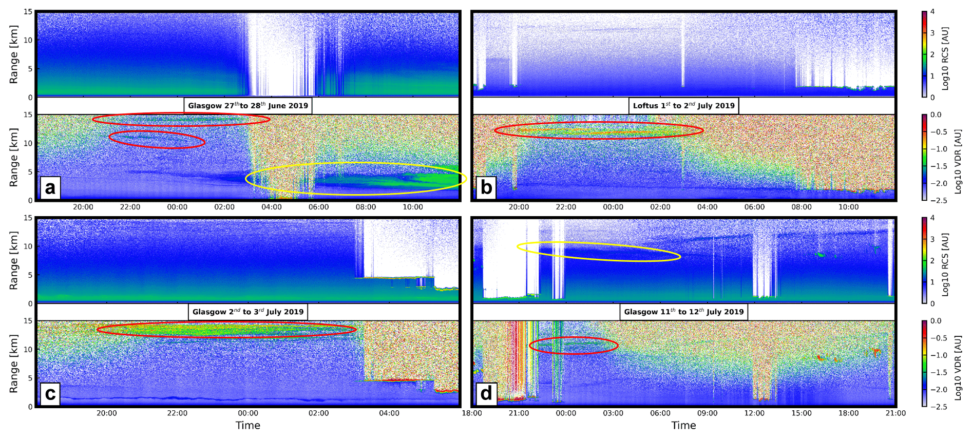
Figure 11 Lidar data from the Met Office lidar sites at Glasgow and Loftus on dates indicated in each axis pair (a), (b), (c) and (d). The upper panel of each pair shows the range-corrected signal [AU], and the lower panel shows the volume depolarisation ratio (VDR) [%].

Rain and low cloud prevented any further measurements in the stratosphere until the evening of 1 July, when several UK network lidars detected aerosol layers between 11.5 and 14 km. Panel (b) shows the data from Loftus for 1 July and into 2 July with the stratospheric layer outlined in red. Again using whole night averages, the mean PDR in these layers was 28±4 % on 1 into 2 July and 32±7 % on 2 and into 3 July (Fig. 11c – layer again outlined in red). This is a marked change from the PDR measured on 27/28 June, and while it is not possible to unambiguously identify the aerosols using the PDR values alone, taken together with the arrival times of simulated BBA and ash clouds, we interpret this change to significantly higher PDR values as the arrival of the ash cloud and the transition of the dominant aerosol type from BBA to volcanic ash. The maximum concentration was observed at Loftus and was 135±78 µg m⁻³.

Low cloud and rain again prevented usable lidar measurements until 11 July when the lidars at Camborne and Glasgow detected an aerosol layer at 9.5 km (outlined in yellow in panel d in Fig. 11) and an optically very thin layer (AOD ≈ 0.005) at 11 km (outlined in red in panel d). The PDR in the lower layer was 0.9±0.2 %, and it was 13±5 % in the higher layer. On 13 July the lidars detected a layer at 13 km with a mean PDR of 1.6±0.4 %. Again, this is a marked change from the previous PDR measurements on 4 July, and when viewed together with the arrival times suggested by the NAME simulations, we interpret this as the arrival of the sulfate cloud, and by 12 July the scattering in the stratospheric layers was dominated by spherical sulfate droplets.

Table 5 Summary of lidar detections. There were marked changes in the PDR measured within the aerosol layers correlated to the dominant aerosol type.

5 Conclusions

The early arrival of aerosol layers over the UK in late June 2019 has been established to be due to the emissions of biomass burning aerosols from intense fires in Alberta that penetrated the tropopause on 17 June 2019. Volcanic ash and sulfur species injected into the upper troposphere and lower stratosphere by the 21 June 2019 eruption of Raikoke reached the UK around 10 d after emission, along with sulfate particles formed by the chemical transformation of volcanic SO₂. The UK lidars were able to make measurements of the particle linear depolarisation ratios and estimate the concentrations within these layers over the UK.

We have presented results from NAME model simulations alongside observations charting the evolution of the aerosol clouds produced by the Raikoke eruption and the Alberta forest fires. The results of the simulations were used to aid in the interpretation of the UK lidar data. A mostly qualitative comparison between the observations and the simulation over the first 5 to 6 d after emission showed that the simulations were representative of the evolution of the aerosol clouds as resolved by the observation and as such could give some insight into the dispersion of the aerosol clouds where no observations were available. This was particularly true of the simulations of the forest fire aerosol cloud. After around 5 to 6 d following emission, the aerosol clouds were no longer visible in the satellite observations. However, the dispersion simulations showed that the BBA arrived over the UK by 27 June, the ash by 1 July and the main bulk of the sulfate aerosol cloud by 11 July, and this was confirmed by the UK lidar network.

By scaling the total mass of BBA released in the simulations so that the air concentration in the distal aerosol cloud over Washington, DC, matches the concentration estimated from the Washington, DC, MPLNET lidar observations, we estimate that the Alberta fires released around 0.2 Tg of fine mode BBA. The mass of volcanic ash released in the simulations (estimated using the Mastin relationship with plume top height) was not scaled to match observations. The simulated ash and sulfate concentrations above Fairbanks, Alaska (400 and 25 µg m⁻³ respectively), were on the same order of magnitude as concentrations estimated from the Fairbanks MPLNET lidar observations (250 and 10 µg m⁻³ for ash and sulfate respectively), suggesting that the mass of ash and SO₂ released in the simulations was reasonably representative of the real value .

The PDRs measured by the UK lidars were 1 % in the sulfate-dominated aerosols, 9 % in the BBA aerosol cloud and 30 % in the volcanic ash. These values did not allow an unambiguous identification of the material within the aerosol clouds, and it was not possible to measure lidar ratios within the layers over the UK. In this respect, NAME simulations were critical in interpreting the observations; they explained the change in the measured PDRs, from around 9 % in the BBA cloud, over 30 % in the ash-containing aerosol cloud and around 1 % in the sulfate dominated aerosol cloud. Importantly, in terms of scientific advice given to the London VAAC, the dispersion simulations showed that the layers detected on 27/28 June 2019 were in fact comprised of BBA particles and not a mix of volcanic ash and sulfate particles. The low aerosol concentrations observed over the UK during the period under study mean that the mistaken identification of the initial aerosol layers at the end of June would have negligible consequences. However, this study shows how the synergy of dispersion modelling and multiple observation sources is important in building a more complete description of aerosol loading.