Projecting ozone hole recovery using an ensemble of chemistry–climate models weighted by model performance and independence

Amos, Matt; Young, Paul J.; Hosking, J. Scott; Lamarque, Jean-François; Abraham, N. Luke; Akiyoshi, Hideharu; Archibald, Alexander T.; Bekki, Slimane; Deushi, Makoto; Jöckel, Patrick; Kinnison, Douglas; Kirner, Ole; Kunze, Markus; Marchand, Marion; Plummer, David A.; Saint-Martin, David; Sudo, Kengo; Tilmes, Simone; Yamashita, Yousuke

doi:https://doi.org/10.5194/acp-20-9961-2020

ACP | Articles | Volume 20, issue 16

Atmos. Chem. Phys., 20, 9961–9977, 2020
https://doi.org/10.5194/acp-20-9961-2020
© Author(s) 2020. This work is distributed under
the Creative Commons Attribution 4.0 License.

Special issue: Chemistry–Climate Modelling Initiative (CCMI) (ACP/AMT/ESSD/GMD...

Atmos. Chem. Phys., 20, 9961–9977, 2020
https://doi.org/10.5194/acp-20-9961-2020
© Author(s) 2020. This work is distributed under
the Creative Commons Attribution 4.0 License.

ACP | Articles | Volume 20, issue 16

Research article 26 Aug 2020

Research article | 26 Aug 2020

Projecting ozone hole recovery using an ensemble of chemistry–climate models weighted by model performance and independence

Matt Amos¹, Paul J. Young^1,2, J. Scott Hosking³, Jean-François Lamarque⁴, N. Luke Abraham^5,6, Hideharu Akiyoshi⁷, Alexander T. Archibald^5,6, Slimane Bekki⁸, Makoto Deushi⁹, Patrick Jöckel¹⁰, Douglas Kinnison⁴, Ole Kirner¹¹, Markus Kunze¹², Marion Marchand⁸, David A. Plummer¹³, David Saint-Martin¹⁴, Kengo Sudo^15,16, Simone Tilmes⁴, and Yousuke Yamashita⁷ Matt Amos et al.

¹Lancaster Environment Centre, Lancaster University, Lancaster, UK
²Centre of Excellence in Environmental Data Science, Lancaster University, Lancaster, UK
³British Antarctic Survey, Cambridge, UK
⁴National Center for Atmospheric Research (NCAR), Boulder, Colorado, USA
⁵Department of Chemistry, University of Cambridge, Cambridge, UK
⁶National Centre for Atmospheric Science (NCAS), Leeds, LS2 9PH, UK
⁷National Institute for Environmental Studies (NIES), Tsukuba, Japan
⁸LATMOS, Institut Pierre Simon Laplace (IPSL), Paris, France
⁹Meteorological Research Institute (MRI), Tsukuba, Japan
¹⁰Institut für Physik der Atmosphäre, Deutsches Zentrum für Luft- und Raumfahrt (DLR), Oberpfaffenhofen, Germany
¹¹Steinbuch Centre for Computing, Karlsruhe Institute of Technology, Karlsruhe, Germany
¹²Institut für Meteorologie, Freie Universität Berlin, Berlin, Germany
¹³Environment and Climate Change Canada, Montreal, Canada
¹⁴CNRM, Université de Toulouse, Météo-France, CNRS, Toulouse, France
¹⁵Graduate School of Environmental Studies, Nagoya University, Nagoya, Japan
¹⁶Japan Agency for Marine-Earth Science and Technology (JAMSTEC), Yokohama, Japan

Correspondence: Matt Amos (matt.r.amos@outlook.com, m.amos1@lancaster.ac.uk)

Received: 28 Jan 2020 – Discussion started: 03 Feb 2020 – Revised: 08 May 2020 – Accepted: 15 Jul 2020 – Published: 26 Aug 2020

Abstract

Back to toptop

Calculating a multi-model mean, a commonly used method for ensemble averaging, assumes model independence and equal model skill. Sharing of model components amongst families of models and research centres, conflated by growing ensemble size, means model independence cannot be assumed and is hard to quantify. We present a methodology to produce a weighted-model ensemble projection, accounting for model performance and model independence. Model weights are calculated by comparing model hindcasts to a selection of metrics chosen for their physical relevance to the process or phenomena of interest. This weighting methodology is applied to the Chemistry–Climate Model Initiative (CCMI) ensemble to investigate Antarctic ozone depletion and subsequent recovery. The weighted mean projects an ozone recovery to 1980 levels, by 2056 with a 95 % confidence interval (2052–2060), 4 years earlier than the most recent study. Perfect-model testing and out-of-sample testing validate the results and show a greater projective skill than a standard multi-model mean. Interestingly, the construction of a weighted mean also provides insight into model performance and dependence between the models. This weighting methodology is robust to both model and metric choices and therefore has potential applications throughout the climate and chemistry–climate modelling communities.

How to cite

How to cite.

Amos, M., Young, P. J., Hosking, J. S., Lamarque, J.-F., Abraham, N. L., Akiyoshi, H., Archibald, A. T., Bekki, S., Deushi, M., Jöckel, P., Kinnison, D., Kirner, O., Kunze, M., Marchand, M., Plummer, D. A., Saint-Martin, D., Sudo, K., Tilmes, S., and Yamashita, Y.: Projecting ozone hole recovery using an ensemble of chemistry–climate models weighted by model performance and independence, Atmos. Chem. Phys., 20, 9961–9977, https://doi.org/10.5194/acp-20-9961-2020, 2020.

1 Introduction

Back to toptop

Global chemistry–climate models (CCMs) are the most comprehensive tools to investigate how the global composition of the atmosphere develops, both naturally and under anthropogenic influence (Flato et al., 2014; Morgenstern et al., 2017; Young et al., 2018). As with projecting climate change, consensus views of the past and potential future evolution of atmospheric composition are obtained from coordinated CCM experiments (Eyring et al., 2008; Lamarque et al., 2013; Morgenstern et al., 2017) and subsequent analysis of the ensemble of simulations (Iglesias-Suarez et al., 2016; Dhomse et al., 2018). Although not a complete sample of structural and epistemic uncertainty, these ensembles are an important part of exploring and quantifying drivers of past and future change and evaluating the success of policy interventions, such as stratospheric-ozone recovery resulting from the Montreal Protocol and its amendments (Dhomse et al., 2018; WMO, 2018). Typically, analysis of an ensemble investigates the behaviour and characteristics of the multi-model mean and the inter-model variance (Solomon et al., 2007; Tebaldi and Knutti, 2007; Butchart et al., 2010), rather than accounting for individual model performance or lack of model independence (Knutti, 2010; Räisänen et al., 2010). Methods to address these shortcomings have been proposed for simulations of the physical climate (e.g. Gillett, 2015; Knutti et al., 2017; Abramowitz et al., 2019), but this topic has received less attention in the atmospheric-composition community. Here, we demonstrate a weighting method for the CCM simulation of Antarctic ozone loss and projected recovery, where the weighting accounts for model skill and independence over specified metrics relevant to polar stratospheric ozone. We apply this to the recent Chemistry–Climate Model Initiative (CCMI) (Morgenstern et al., 2017) ensemble and demonstrate the impact of the weighting on estimated ozone hole recovery dates.

Many years of scientific studies and assessments have tied stratospheric-ozone depletion to the anthropogenic emission and subsequent photochemistry of halogen-containing gases, such as chlorofluorocarbons (CFCs), hydrofluorocarbons (HCFCs) and halons (WMO, 2018). This science guided the development of the Montreal Protocol and its subsequent amendments to limit and ban the production of these ozone-destroying gases, and stratospheric ozone is now thought to be recovering (Solomon et al., 2016; Chipperfield et al., 2017). Of particular concern is the Antarctic “ozone hole”: a steep decline in high-latitude stratospheric ozone during austral spring that can reduce ozone concentrations to near zero at particular altitudes, driven by polar nighttime chemistry, cold temperatures and heterogeneous catalysis on polar stratospheric clouds (PSCs) (Solomon, 1999). While the ozone hole continues to appear in each austral spring, it appears to be showing signs of recovery (Langematz et al., 2018). The strong cooling associated with Antarctic ozone depletion (Thompson and Solomon, 2002; Young et al., 2012) has driven circulation changes in the stratosphere and in the troposphere, particularly in austral summer. This has notably included an acceleration and poleward movement of the southern high-latitude westerly winds and associated storm tracks (Son et al., 2008; Perlwitz et al., 2008), leading to summertime surface climate changes through many lower-latitude regions including the tropics (Thompson et al., 2011).

The recovery process is slow due to the long atmospheric lifetimes of ozone-depleting substances and could be hampered by releases of ozone-depleting substances (ODSs) not controlled by the Montreal Protocol, such as short-lived halogens (Claxton et al., 2019; Hossaini et al., 2019) or nitrous oxide (Portmann et al., 2012; Butler et al., 2016), or instances of non-compliance, such as the recent fugitive emissions of CFC-11 (Montzka et al., 2018; Rigby et al., 2019). Recovery itself is often defined as the date at which the ozone layer returns to its 1980 levels, and this is the benchmark used by the World Meteorological Organization (WMO; WMO, 2018) to assess the progress due to the implementation of the Montreal Protocol.

The assessment of when the ozone layer will recover is conducted using an ensemble of chemistry–climate models, forced by past and projected future emissions of ozone-depleting substances (ODSs) and climate forcers (Eyring et al., 2010; Dhomse et al., 2018). Such ensembles are used to establish the robustness of the model results for a particular scenario: when several models agree, the prevailing assumption is that we can have greater confidence in the model projections. Yet, there has been much discussion about how true this assumption is (Tebaldi and Knutti, 2007; Sanderson et al., 2015 b; Abramowitz et al., 2019). In an ideal scenario, every model within an ensemble would be independent and have some random error. In this case, we would expect that increasing the ensemble size would decrease the ensemble uncertainty and allow us to better constrain the mean value. However, in modern model inter-comparison projects this is not the case: although often developed independently, models are not truly independent, often sharing components and parameterisations (Knutti et al., 2013); models are not equally good at simulating the atmosphere (Reichler and Kim, 2008; Bellenger et al., 2014); and lastly, models do not have a predictable random error but instead have layers of uncertainty extending from uncertainties in parameterising sub-grid processes (Rybka and Tost, 2014) to structural uncertainties from the design of the model (Tebaldi and Knutti, 2007; Knutti, 2010).

Given these issues, there is currently no consensus on how best to combine model output when analysing an ensemble. Probably the most widely used and simplest is to take a multi-model mean where each model contributes equally, and indeed it has also been established that an ensemble mean performs better than any single model (Gleckler et al., 2008; Reichler and Kim, 2008; Pincus et al., 2008; Knutti et al., 2010). A more sophisticated method is to weight individual ensemble members, accounting for model performance as well as the degree of a model's independence. Weighting methods of various forms have been developed and implemented on global physical climate model ensembles (Tebaldi et al., 2005; Räisänen et al., 2010; Haughton et al., 2015; Knutti et al., 2017) but seldom for atmospheric composition. In most cases the weights are calculated from comparison of model hindcasts to observational data, either for a single variable of interest or over a suite of diagnostics. Additionally, reliability ensemble averaging (REA) (Giorgi and Mearns, 2002) is an alternative weighting technique which gives higher weights to those models near the multi-model mean. The main motivation for using a weighted mean is to encapsulate model skill and model independence such that we down-weight models which perform less well and/or are more similar.

Quantifying model skill (or performance) against comparable observations forms an important part of the validation and analysis of multi-model ensembles (Gleckler et al., 2008; Flato et al., 2014; Harrison et al., 2015; Hourdin et al., 2017; Young et al., 2018). Many CCM inter-comparison projects feature validation and assessment through the use of observation-based performance metrics, which may capture model performance for particular atmospheric variables (e.g. temperature, chemical species concentrations and jet position) or be a more derived quantity which gets closer to evaluating the model against the process it is trying to simulate (e.g. ozone trends versus temperature trends, chemical species correlations, and relationships of chemistry–meteorology and transport ) (Eyring et al., 2006; Waugh and Eyring, 2008; Christensen et al., 2010; Lee et al., 2015). Performance metrics are chosen based upon expert knowledge of the modelled system to ensure that metrics are highly related to the physical or chemical processes that the models are being evaluated on.

In this study we develop a weighting methodology, originally presented by Sanderson et al. (2017) and Knutti et al. (2017), for CCM ensembles that accounts for model performance and model independence. We apply it to the important issue of estimating Antarctic ozone recovery using several well-established metrics of model performances, where previously only unweighted means have been used. We first describe our weighting framework in Sect. 2, before describing the model and observational data in Sect. 3. Section 4 presents the application of the weighting framework to Antarctic ozone depletion and the corresponding results. Sections 5 and 6 present a summary and our conclusions.

2 The model-weighting framework

Back to toptop

In this study, we develop and exploit a framework to calculate model weights based on recent work in the physical-climate-science community (Sanderson et al., 2015 a, b, 2017; Knutti et al., 2017; Lorenz et al., 2018; Brunner et al., 2019). Here, for an ensemble of N models, the weight for model i (w_i) is given by

\begin{matrix} (1) & w_{i} = \frac{\exp (- \frac{D_{i}^{2}}{n_{i} σ_{D}^{2}})}{1 + \sum_{j \neq i}^{N} \exp (- \frac{S_{i j}^{2}}{n_{i} σ_{S}^{2}})} . \end{matrix}

The numerator captures the closeness of the model to observations. $D_{i}^{2}$ is the squared difference between a model and the corresponding observation, which is a measure of performance. The denominator captures the closeness of a model to all other models by comparing the squared difference between them ( $S_{i j}^{2}$ ). Both σ_D and σ_S are constants which allow for tuning of the weighting to preference either independence or performance (see discussion below). Put more simply, a model has a larger weighting if it closely matches observations and is suitably different to the other models in the ensemble. Finally, Eq. (1) differs from similar versions (e.g. Knutti et al., 2017) through the addition of n_i, which is the size of the data used to create the weighting. This could be the amount of grid points for a spatial field, the number of points in a time series or just one for a single-valued statistic, and it normalises the data by length allowing for comparison between models and variables with time series of different length- and time-invariant parameters.

Investigating and evaluating a phenomenon or complex process often relies on identifying multiple metrics since it can only be partially expressed by any single variable. Expert understanding of the physical process is needed to select a set of relevant metrics with which to develop the process-based weighting. Including multiple metrics, provided they are not highly correlated, has the further benefit of giving less weight to models which perform well but do so for the wrong reasons. In this framework, ensuring that these metrics influence the weighting proportionally is done by normalising the model data using a min–max scaling between 0 and 1.

When combining multiple metrics into a weighting, the weight of the ith model can be found from

\begin{matrix} (2) & w_{i} = \frac{(\sum_{k = 1}^{M} \exp (- \frac{D_{i k}^{2}}{n_{i k} σ_{D}^{2}}))}{(M + \sum_{k = 1}^{M} \sum_{j \neq i}^{N} \exp (- \frac{S_{i j k}^{2}}{n_{i k} σ_{S}^{2}}))}, \end{matrix}

where M is the total number of metrics and k is the index of the metric. Note that the summation is performed separately over the numerator and the denominator. This means that we calculate the performance and independence scores over all the metrics combined before merging the scores to create the final weighting, which, as before, is normalised over all the models to sum to 1.

We take the combined weights for each model and apply them to our parameter or process of interest (the evolution of stratospheric ozone here). As with the metrics this parameter need not be a time series and could be a spatial distribution or a single measure. The weighted projection is therefore $x = \sum_{i = 1}^{N} w_{i} x_{i}$ , where x_i is an individual model projection and w_i is the associated weight.

2.1 Choosing sigma values

The two scaling parameters (σ_S and σ_D) represent a length scale over which two models, or a model and observation, are deemed to be in good agreement. For example, a large σ_S would spread weight over a greater number of models, as more models would lie within the length scale of σ_S. On the other hand, a small σ_S sets a higher tolerance for measuring similarity. The choice of the sigma values needs to be considered carefully to strike a balance between weighting all models equally, thus returning to a multi-model mean, versus weighting just a few selected models. As the same values of sigma apply across all metrics, it is necessary for the data to be normalised to the same values, ensuring that metrics impact the weightings equally. Figure 1 shows how the weighting function depends on σ_S, σ_D, model performance and model independence.

As noted in Knutti et al. (2017) there is not an objective way of determining optimal sigma values. Our method of selecting appropriate parameter values was to consider a training and a testing set of data, much like a machine learning problem. We determined the values of sigma using the training data, which in this case is the refC1SD simulations such that the weighted training data gave a good fit to the observations. The testing data (refC2 simulations) allowed us to test the weights and sigma values out of the temporal range of the training data, which avoids performing testing on data that were used to tune the parameters.

https://acp.copernicus.org/articles/20/9961/2020/acp-20-9961-2020-f01

Figure 1Panel (a) shows the overall weighting function w_i (Eq. 1), plotted for 11 models (N=11) with σ_D=0.1 and σ_S=0.1. Panel (b) shows the contribution to the weighting due to model performance (at $S_{i j}^{2} / n_{i} = 1$ ), and panel (c) shows the contribution due to model independence (at $D_{i}^{2} / n_{i} = 10^{- 4}$ ). A model which has higher independence and higher skill receives a larger weight. For the weight due to performance (a) we can see that the weight equals e⁻¹ when $D_{i}^{2} / n_{i} = σ_{D}^{2}$ . This shows how σ_D acts as a length scale that determines how close a model has to be to observations to receive weight. σ_S works similarly, setting the length scale that determines similarity.

Download

3 Applying the weighting framework to the Antarctic ozone hole

Back to toptop

We demonstrate the applicability of this weighting framework by applying it to the important and well-understood phenomenon of the Antarctic stratospheric ozone hole, for which we can use several decades of suitable observations to weight the models. Below, we describe the model and observation data used and the metrics selected, against which we measure model performance and independence.

3.1 Model and observation data sources

CCM output was taken from the simulations conducted under Phase 1 of the Chemistry–Climate Model Initiative (CCMI) (Morgenstern et al., 2017, and references therein), which represents an ensemble of 20 state-of-the-art CCMs (where chemistry and atmospheric dynamics are coupled) and chemistry transport models (CTMs, where the dynamics drives the chemistry, but there is no coupling). A detailed description of the participating models is provided by Morgenstern et al. (2017), and here we briefly review their overarching features. Most models feature explicit tropospheric chemistry and have a similar complexity of stratospheric chemistry, though there is some variation in the range of halogen source gases modelled. Horizontal resolution of the CCMs ranges from between $1.125^{\circ} \times 1.125^{\circ}$ and $5.6^{\circ} \times 5.6^{\circ}$ . Vertically, the atmosphere is simulated from the surface to near the stratopause by all models, and many also resolve higher in the atmosphere. Vertical resolution varies throughout the models, both in the number of levels (34 to 126) and their distribution. All models simulate the stratosphere, although they differ in whether they have been developed with a tropospheric or stratospheric science focus.

Imai et al. (2013)Akiyoshi et al. (2016)Tilmes et al. (2015)Marsh et al. (2013)Solomon et al. (2015)Garcia et al. (2017)Sudo et al. (2002)(Sudo and Akimoto, 2007)Watanabe et al. (2011)Sekiya and Sudo (2012)Sekiya and Sudo (2014)Jonsson et al. (2004)Scinocca et al. (2008)Michou et al. (2011)Voldoire et al. (2013)Jöckel et al. (2010)Jöckel et al. (2016)Marchand et al. (2012)Szopa et al. (2013)Dufresne et al. (2013)Deushi and Shibata (2011)Yukimoto (2011)Yukimoto et al. (2012)Morgenstern et al. (2009)Bednarz et al. (2016)

Table 1The CCMI model simulations used in this analysis and their key references.

^a Represents the simulations used in the similarity analysis but that did not form part of the model weighting.

Download Print Version | Download XLSX

We focus on two sets of simulations, called refC1SD and refC2, and for the weighting analysis we only consider models which ran both simulations. Table 1 details the exact model simulations used. The refC1SD simulations cover 1980–2010 and represent the specified-dynamics hindcast, where the models' meteorological fields are nudged to reanalysis datasets in order that the composition evolves more in line with the observed inter-annual variability of the atmosphere. In addition to being nudged by meteorology, the refC1SD runs are forced by realistically varying boundary conditions, including greenhouse gas (GHG) concentrations, ODS emissions, and sea surface temperatures (SSTs) and sea-ice concentrations (SICs). The refC1SD simulations are used to create the model weightings, since these are the models' best attempt at replicating the past, giving reasonable confidence that any down weighting arises due to poorer model performance or strong inter-model similarity. It must be noted that the nudging process is not consistent across the models (Orbe et al., 2018), and we should be mindful that it has the capability to influence the weighting. We discuss the choice to use refC1SD simulations in greater detail in Sect. 5.

The refC2 simulations cover 1960–2100 and are used to construct weighted projections of Antarctic ozone recovery, using the weights calculated from refC1SD. The forcing from GHGs and anthropogenic emissions follows the historical scenario conditions prescribed for the fifth Coupled Model Inter-comparison Project (CMIP5) (Lamarque et al., 2010) up to the year 2000 and subsequently follows RCP6.0 (representative concentration pathway) for GHGs and tropospheric pollutant emissions (van Vuuren et al., 2011); the ODS emissions follow the World Meteorological Organization A1 halogen scenario (WMO, 2011). From CCMI this is the only scenario which estimates the future climate change and developments to stratospheric ozone.

Mears and Wentz (2009)Bodeker et al. (2018)Froidevaux et al. (2015)Berrisford et al. (2011)

Table 2The observational products and respective variables used to construct metrics on which to weight the models. MSU: Microwave Sounding Unit. NIWA-BS: National Institute of Water and Atmospheric Research – Bodeker Scientific. GOZCARDS: Global OZone Chemistry And Related trace gas Data records for the Stratosphere. ERA-Interim: European Centre for Medium-Range Weather Forecasts – ECMWF – Reanalysis.

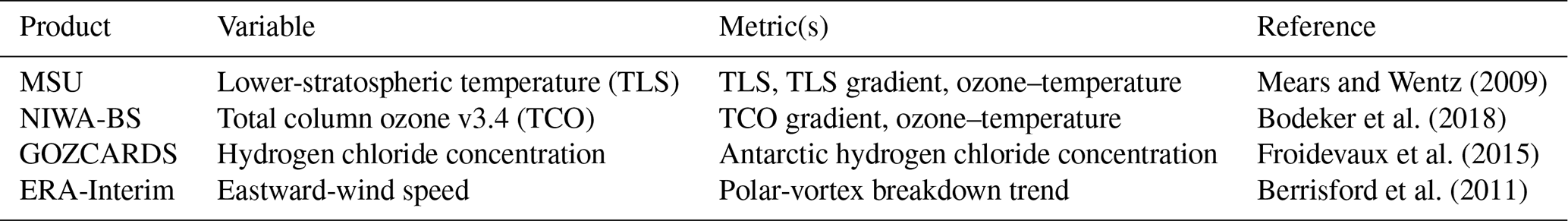
Download Print Version | Download XLSX

Model performance was evaluated against a series of well-accepted metrics (see below), drawing from widely used observational and reanalysis datasets listed in Table 2. Assessing models and ensembles using observational data is a principal way of validating models (Eyring et al., 2006; Waugh and Eyring, 2008; Dhomse et al., 2018), and this is the methodology we follow, with the addition that we create the weights based upon this skill, alongside model independence.

Like many ozone recovery studies, we utilise TSAM (time series additive modelling) (Scinocca et al., 2010) to quantify projection confidence, which produces smooth estimates of the ozone trend whilst extracting information about the inter-annual variability. Here, the TSAM procedure involves finding individual model trends for the refC2 simulations by removing the inter-annual variability using a generalised additive model. Each model trend is then normalised to its own 1980 value. The weighted mean (WM) is created by summing model weights with individual model trends. Two uncertainty intervals are created: a 95 % confidence interval, where there is a 95 % chance that the WM lies within, and a 95 % prediction interval, which captures the uncertainty of the WM and the inter-annual variability.

3.2 Metric choices – how best to capture ozone depletion

The first step in the weighting process is to identify the most relevant processes that affect Antarctic ozone depletion to allow for appropriate metric choice. Suitable metrics require adequate observational coverage and for the models to have outputted the corresponding variables. The metrics we chose are as follows:

Total ozone column gradient: This is the first derivative with respect to time of the total ozone column. Given the discontinuity in the total ozone column record, the years 1992–1996 are excluded. It is a southern polar cap (60–90^∘ S) average over austral spring (October and November). September is not included due to discontinuous coverage in the observations.
Lower-stratospheric temperature: The lower-stratospheric temperature for all of the models are constructed using the MSU TLS-weighting function (Mears and Wentz, 2009). The MSU dataset extends to 82.5^∘ S, and therefore the southern polar cap average ranges from 60 to 82.5^∘ S and is temporally averaged over austral spring (Sept, Oct, Nov).
Lower-stratospheric temperature gradient: This is the first derivative with respect to time of the lower-stratospheric temperature found above.
Breakdown of the polar vortex: The vortex breakdown date is calculated as when the zonal mean wind at 60^∘ S and 20 hPa transitions from eastward to westward as per Waugh and Eyring (2008). We find the trend of the breakdown date between the years 1980 and 2010, and the gradient of the trend forms the polar-vortex breakdown metric.
Ozone–temperature gradient: Both the lower-stratospheric temperature and the total ozone column are separately averaged over 60 to 82.5^∘ S, and the October and November mean was taken. We determined a linear relationship between temperature and total ozone column, and the gradient of this linear relationship forms the ozone–temperature metric (Young et al., 2013).
Ozone-trend–temperature-trend gradient: This is similar to the metric above except that we first calculated the time derivative of the total ozone column and temperature polar time series before calculating the linear relationship. The gradient of the linear relationship is the total-ozone-column-trend–temperature-trend gradient metric.
Hydrogen chloride: The hydrogen chloride concentration was averaged over the austral spring months and over the southern polar cap, for areas which have observational coverage. We consider a pressure range of 316 to 15 hPa to capture the concentration in the lower stratosphere.

These metrics capture two of the main features of ozone depletion, namely: (1) the decrease in temperature over the poles caused by the depletion of ozone and (2) the breakdown of the vortex which has a major role of isolating the ozone-depleted air mass. The chlorine metric encapsulates the anthropogenic release of ODSs and the main chemical driver of ozone depletion. Ozone–temperature metrics allow us to look at model success in reproducing the temperature dependency in ozone reaction rates and stratospheric structure. By looking at the instantaneous rate of change as well as the overall trends, we can gather a picture of both short-term and long-term changes for a range of chemical and dynamical processes.

The metrics are not highly correlated, except for the total ozone column gradient and the lower-stratospheric temperature gradient, which are correlated because of the strong coupling of ozone and temperature in the stratosphere (e.g. Thompson and Solomon, 2008). Although this could be cause to discard one of the metrics, to avoid potential double counting, we retain and use both to weight because the models may not necessarily demonstrate this coupling that we see in observations. By considering this variety of metrics, the approach aims to demonstrate that models do not just get the “right” output but that they do so for the right reasons.

3.3 Evaluating the weighting framework

Two types of testing were used to investigate the usefulness of the weighted prediction and to validate metric choices. Firstly, we performed a simple out-of-sample test on the weighted prediction against the total ozone column observations from NIWA-BS. Although the weights are generated from comparison between the specified-dynamics runs (refC1SD) and observations, it does not necessarily follow that the weighted projection created using the free-running (refC2) runs will be a good fit for the observations. To test this, we compared the refC2 multi-model mean and weighted projection to the observations. Due to the large inter-annual variability in the total column ozone (TCO) observations, we do not expect the weighted average to be a perfect match; after all, free-running models are not designed to replicate the past. However, we need to test the level of agreement between the weighted mean and the observations for an out-of-sample period (2010–2016). This serves a secondary purpose of determining transitivity between the two model scenarios used, i.e. that the weightings found from refC1SD apply to refC2.

Secondly, we used a perfect-model test (also known as model-as-truth or a pseudo-model test) to determine whether our weighting methodology is producing valid and robust projections. In turn, each model is taken as the pseudo truth and weightings are found in the same way as described in Sect. 2 except that the pseudo truth is used in place of observations. From these weightings we can examine the skill with which the weighted mean compares to the pseudo truth. We are normally limited to a single suite of observations, but a perfect-model test allows us to test our methodology numerous times using different pseudo truths, demonstrating robustness.

Perfect-model testing also allows us to test transitivity between scenarios, since, unlike with the obvious temporal limit on observations, the pseudo truth exists in both the hindcast and forecast. If a weighting strategy produces weighted means which are closer to the pseudo truth than a multi-model mean, then we can have some confidence that we can apply a weighting across model scenarios. Herger et al. (2019) compare the perfect-model test to the cross validation employed in statistics but note that although necessary, perfect-model tests are not sufficient to fully show out-of-sample skill which in this case is scenario transitivity. It should be backed up by out-of-sample testing as described above.

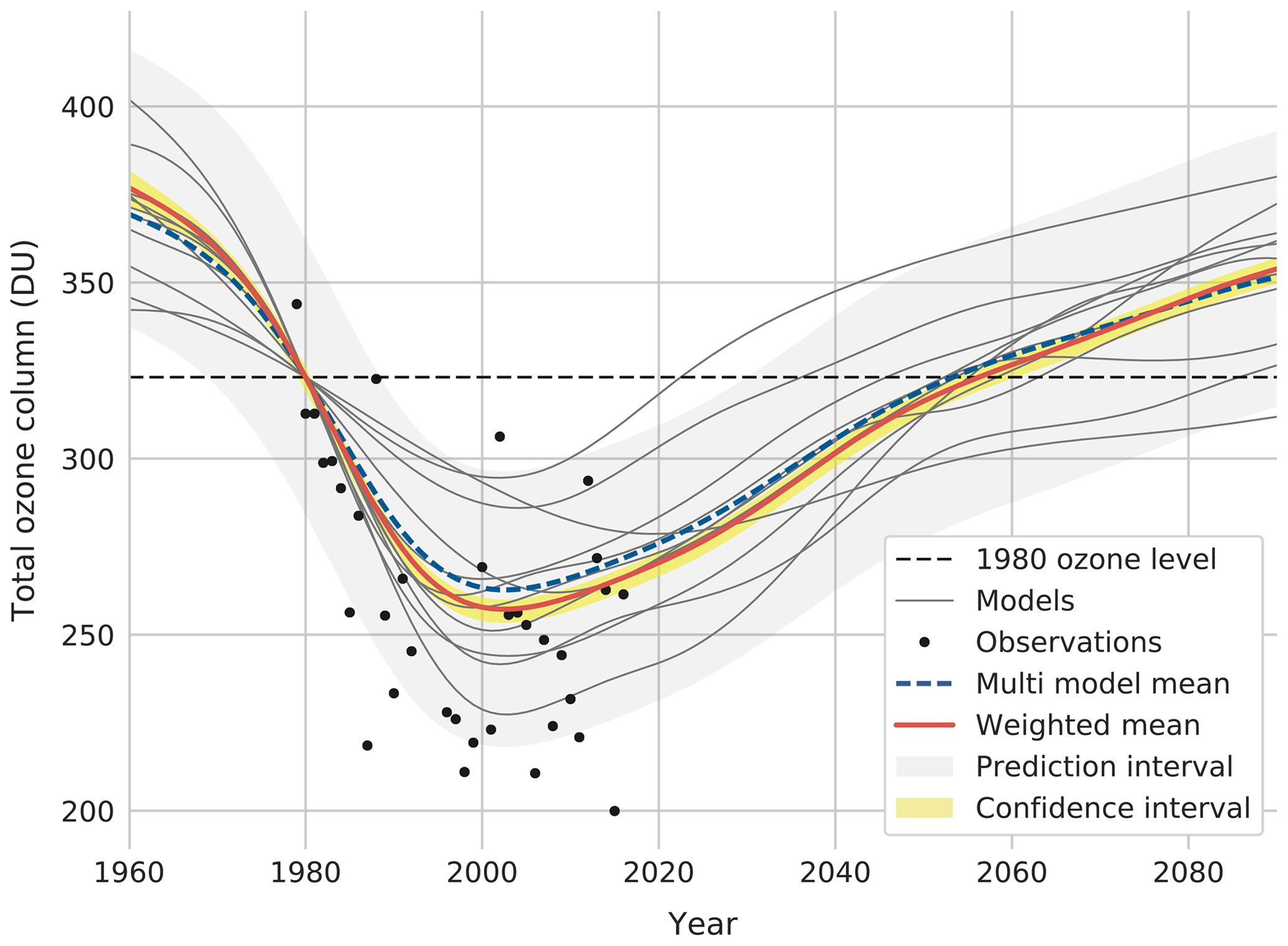
https://acp.copernicus.org/articles/20/9961/2020/acp-20-9961-2020-f02

Figure 2Antarctic (60–90^∘ S) October TCO. The weighted mean (refC2 simulations weighted upon refC1SD performance and independence) is shown in red; the multi-model mean (refC2 simulations) is shown in blue; and individual refC2 model trends are shown in grey. The NIWA-BS observations are shown in black. All model projections and ensemble projections are normalised to the observational 1979–1981 mean shown as the black dashed line. The 95 % confidence and prediction intervals for the weighted mean are also shown with shading.

Download

4 Applying the weighting framework to Antarctic ozone simulations

Back to toptop

4.1 Antarctic ozone and recovery dates

Figure 2 shows the October weighted-mean (WM) total column ozone (TCO) trend from the refC2 simulations for the Antarctic (60–90^∘ S). The weights are calculated using Eq. (2) and are based on both model performance and independence. All models simulate ozone depletion and subsequent recovery but with large discrepancies in the absolute TCO values and the expected recovery to 1980 levels (see Dhomse et al., 2018), from here on referred to as D18. The WM and multi-model mean (MMM) are similar, given the small number of models considered from the ensemble (N=11). At maximum ozone depletion, around the year 2000, the WM projects a significantly lower ozone concentration (5 DU; Dobson unit) than the MMM. This steeper ozone depletion seen in the WM fits the observations better than the MMM, although the modelled inter-annual variability seems to underpredict the observations.

The WM predicts a return to 1980 TCO levels by 2056 with a 95 % confidence interval (2052–2060). For comparison the recovery dates presented in D18 were 2062 with a 1σ spread of 2051–2082. Although taken from the same model ensemble (CCMI), the subset of models in this analysis is smaller than that used in D18, meaning that difference in recovery dates between the two works is attributable to both the methodology and the models considered. The smaller number of models used in this study could lead to a narrower confidence interval than the one reported in D18.

The confidence interval for recovery dates is formed from the predictive uncertainty in the WM from the TSAM (for which the 95 % confidence interval is 2054–2059) and the uncertainty associated with the weighting process. Choices made about which models and metrics to include influence the return dates and therefore introduce uncertainty. This is similar to the concept of an “ensemble of opportunity”, which is that only modelling centres with the time, resources or interest take part in certain model ensembles. To quantify this uncertainty, we performed a dropout test where a model and a metric were systematically left out of the recovery date calculation. This was done for all combinations of models (N=11) and metrics (M=7), providing a range of 77 different recovery dates between 2052 and 2058. Combining the TSAM and dropout uncertainties produces a 95 % confidence interval of 2052–2060. We additionally tested dropping out up to three metrics at a time and observed that the confidence interval did not notably increase in size.

Figure 3 shows the model weights for individual metrics and in total as found using Eqs. (1) and (2). Good agreement is shown between the models for the metrics of lower-stratospheric temperature, the temperature gradient and the TCO gradient. There is one exception of UMUKCA-UCAM which exhibits a colder pole compared to the ensemble and observations. Resultantly, UMUKCA-UCAM is down-weighted for its lower performance at replicating the historic lower-stratospheric temperature. Dissimilarity to the rest of the ensemble will contrastingly increase the weighting but to a lesser effect than the down weighting for performance, due in part to the values of the sigma parameters. In spite of a bias in absolute lower-stratospheric temperature, UMUKCA-UCAM does reproduce the trend in the lower-stratospheric temperature with similar skill to the other models.

Due to the nudging of temperature that takes place in most of the specified-dynamics simulations, we would expect stratospheric temperatures to be reasonably well simulated. However, variation exists in nudging methods in addition to inter-model differences, and this leads to part of the variability in weights (Orbe et al., 2018; Chrysanthou et al., 2019). For the ozone–temperature metrics, which although formed from variables linked to nudged fields are more complex in their construction, we see a much less uniform spread of weights. Furthermore, for processes not directly linked to nudged variables (hydrogen chloride, ozone and the polar-vortex breakdown trend), there is much less agreement between models. This is captured in the weights of these metrics which show just a few models possessing large weights.

The total weighting, formed from the mean of individual metric weights per model, is largely influenced by CNRM-CM5-3, which has a weight of 0.27 (297 % of the value of a uniform weighting). The CNRM-CM5-3 simulations are more successful at simulating metrics whilst being reasonably independent from other models, leading to a weight with greater prominence than the other models. This does not mean that CNRM-CM5-3 is the most skilful model. For example, if two nearly identical models had the highest performance, their final weights would be much lower, as they would be down-weighted for their similarity. All models are contributing towards the weighted ensemble mean providing confidence that our weighting methodology is not over-tuned and returning model weights of zero. The lowest total model weight is 45 % of the value of a uniform weighting.

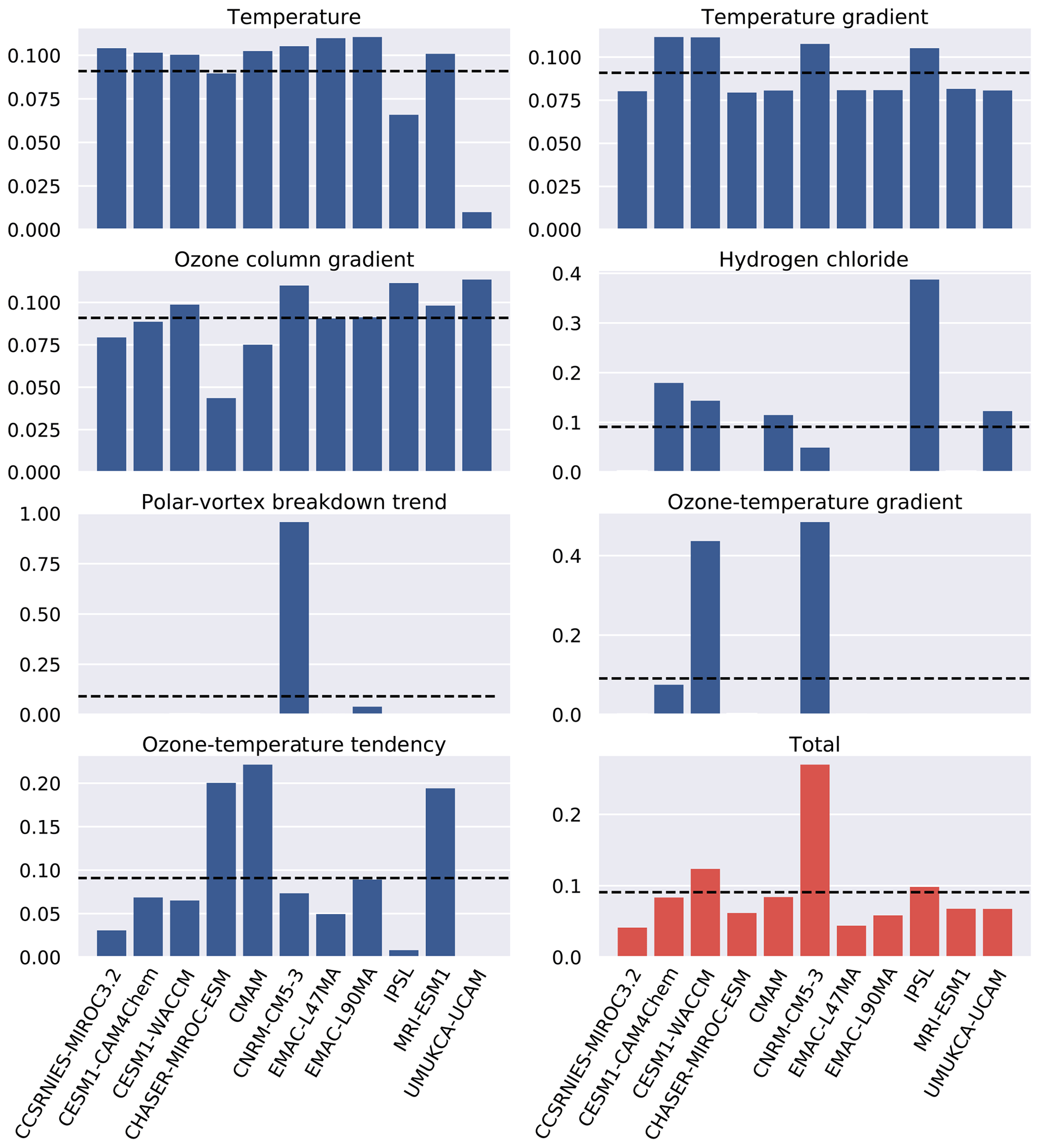
https://acp.copernicus.org/articles/20/9961/2020/acp-20-9961-2020-f03

Figure 3Model weights for each of the seven metrics are all shown in blue. The weights account for both performance and independence and are found using Eq. (1). The total weights, as found from Eq. (2), are shown in red and were the weights used to construct the weighted mean shown in Fig. 2. The black dashed line indicates a uniform weighting as prescribed by a multi-model mean.

Download

https://acp.copernicus.org/articles/20/9961/2020/acp-20-9961-2020-f04

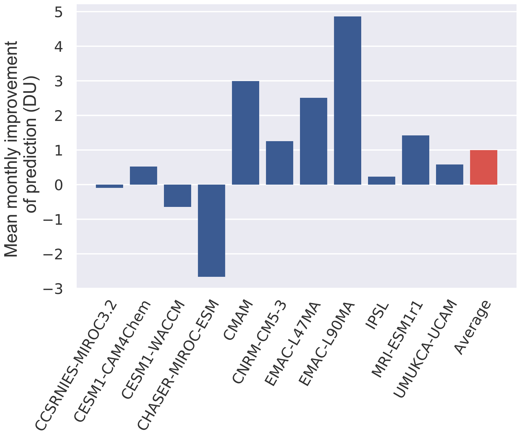
Figure 4Results of the perfect-model test. The mean monthly improvement in the Antarctic October TCO projection (1960–2095) of the WM compared to the MMM for each model taken as the pseudo truth. The average shown in red is the improvement across all the perfect-model tests. No conclusions about overall model skill should be drawn from this plot.

Download

4.2 Testing the methodology

We performed a perfect-model test (Sect. 3.3) to assess the skill of the weighted-mean projection, the results of which are shown in Fig. 4. The perfect-model test shows that, on average, using this weighting methodology produces a WM which is closer to the “truth” than the MMM by 1 DU. In addition to improvements in projections, the pseudo recovery dates are better predicted on average, with a maximal improvement of 6 years.

Three models, when treated as the pseudo truth, do not show an improvement of the WM with respect to the MMM. Note that this is not poor performance of the model in question, but it is rather that the weighting methodology does not do an adequate job of creating a weighted projection for that model as the pseudo truth. Using CHASER-MIROC-ESM as the pseudo truth gives a worse WM projection than if we used the MMM. However, the average correlation between the CHASER-MIROC-ESM-simulated TCO and other models in the ensemble is the lowest at 0.65, compared to the average ensemble cross-correlation score of 0.81. Since a weighted mean is a linear combination of models in the ensemble, it is understandable that models with low correlation to CHASER-MIROC-ESM will be less skilful at replicating its TCO time series. This is why an improvement is not seen for CHASER-MIROC-ESM as the pseudo truth in the perfect-model testing.

We also performed out-of-sample testing on the WM projection for the years 2011–2016 inclusive by comparing it to the TCO observational time series, which was smoothed as described in Sect. 3.1 to remove inter-annual variability. The mean squared error (MSE) was used as the metric for goodness of fit. This range of years is chosen, as it is the overlap between the TCO observations and the years not used in the creation of the weighting. The MSE of the WM is on average 202 DU² less than the MMM per year, and the MSE values were 1510 and 2720 DU² for the WM and MMM respectively for the out-of-sample period.

https://acp.copernicus.org/articles/20/9961/2020/acp-20-9961-2020-f05

Figure 5Inter-model similarity across all refC1SD models as calculated by Eq. (3). A similarity of 1 denotes models which are identical for all the metrics, whereas a lower similarity shows a greater independence. The orange boxes highlight the model most similar to the model on the y axis.

Download

4.3 Model independence

The current design of model inter-comparison projects does not account for structural similarities in models, ranging from sharing transport schemes to entire model components. Therefore, a key part of generating an informed weighting is considering how alike any two models are. The weighting scheme presented here accounts for model independence through the denominator in Eq. (1).

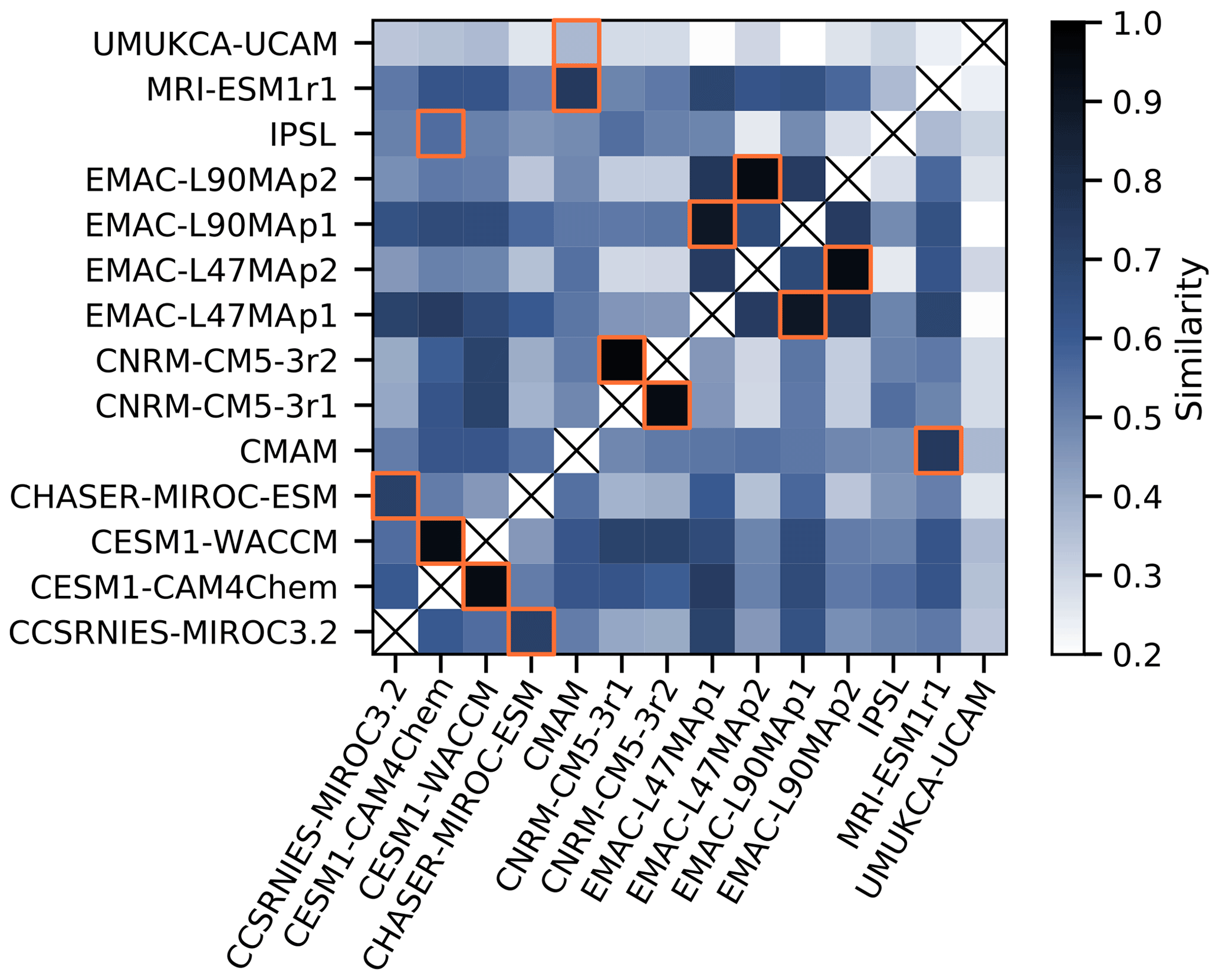
The refC1SD scenario from CCMI consists of 14 different simulations, some of which are with different models, whereas others are just different realisations of the same models. Note that there are more models used here than in the creation of the Antarctic ozone projection. This is because for the weighted projection we require both a refC1SD and a refC2 simulation for each model, but for similarity analysis we can use all the refC1SD simulations. For these model runs we calculated a similarity index s_ij (shown in Eq. 3), which is the similarity between models i and j averaged across all the performance metrics, where n_k is the size of the data for metric k.

\begin{matrix} (3) & s_{i j} = \frac{1}{M} \sum_{k = 1}^{M} \exp (\frac{- S_{i j k}^{2}}{n_{k} σ_{S}^{2}}) \end{matrix}

Similarities between all refC1SD models are shown in Fig. 5. We also found the maximum value of s_ij for each model, indicating the model which model i is most similar to. The most alike models are the two realisations of CNRM-CM5-3, which are the same models running with slightly different initial conditions. We also see high similarity between the two variations of the CESM model, CESM-WACCM and CESM-CAM4Chem. CESM1-CAM4Chem is the low-top version of CESM1-WACCM, meaning that up to the stratosphere the two models should be much alike (Morgenstern et al., 2017). Analysing the EMAC models this way presents an interesting observation: changing the nudging method has a greater impact on model similarity than changing the number of vertical levels (the difference between EMAC-L47MAr1i1p1 and EMAC-L47MAr1i1p2, and likewise the 90-level model variant, is that the p1 variant additionally nudges to the global mean temperature; Jöckel et al., 2016). CHASER-MIROC-ESM and CCSRNIES-MIROC3.2 are two other models which are identified as similar albeit at a lower value. Considering that these two models are built upon the same MIROC general circulation model, it is not a surprise that we see a similarity. The fact that the weighting framework can identify all of the models with known similarities (same institution or realisations) confirms confidence in the methodology and means that we are down weighting similar models.

5 Discussion

Back to toptop

The projection of the ozone hole recovery date presented here makes use of an ensemble of the latest generation of CCMs and a weighting methodology that accounts for complexities within model ensembles. While the ozone recovery date found in this work (2056) is different to that found by Dhomse et al. (2018) (2062), these two dates are not easily comparable, as they are created from different subsets of the same ensemble. For our subset of models, the MMM recovery date was 3 years earlier (2053) than the WM. Although the return dates are not significantly different, for the period of peak ozone depletion (especially between 1990 and 2030), the MMM projection is significantly different to the WM. As the model subsets in this work, for the WM and MMM remain the same, the variation in the projections is entirely due to the construction of the WM.

The CNRM-CM5-3 model received the largest weight of 0.27, giving it 3 times the influence in the WM than in the MMM. Initially this may seem as if we are placing too much importance on one model, but consider that in a standard MMM, a model which runs three simulations with different combinations of components will have 3 times the influence of a model with a single simulation. Furthermore, CNRM-CM5-3 is not weighted higher, because it ran more simulations; it is weighted higher because it is skilful at simulating hindcasts whilst maintaining a level of independence.

Central to the weighting methodology is the selection of metrics requiring expert knowledge. The set of metrics we chose was grounded in scientific understanding and produce a good improvement of the weighted projection compared to the MMM. There are numerous other metrics of varying complexity which could be considered, such as the size of the ozone hole or the abundance of polar stratospheric clouds. These extra metrics could improve the model weighting and give a more accurate projection, but testing an exhaustive collection of metrics was not our aim, and there are not always appropriate measurements to validate the metrics with. We have shown a weighting framework which improves upon the current methodology for combining model ensembles and is also flexible and adaptable to whichever metric choices the user deems reasonable. Furthermore, the low range in return dates produced from the dropout testing shows that the results produced in this weighting framework are robust to metric and model choices. This is a desirable effect of a methodology to provide stable results irrespective of fluctuations in the input. It is reassuring to know that the methodology is robust to metric choices, as we are often constrained by the availability of observational data. In this work we benefit from the decades of interest in polar ozone which have led to datasets of a length suitable for constructing model weights. This highlights the importance of continued production of good observational datasets because, although perfect-model testing allows us a form of testing which forgoes the need for observations, weighting methodologies must be grounded in some estimate of the truth.

Abramowitz et al. (2019) discuss approaches for assessing model dependence and performance and mention caveats around the notion of temporal transitivity: is model behaviour comparable between two distinct temporal regions? Here, we rephrase the question to be the following: are the weights generated from the hindcast scenario relevant and applicable to the forecast scenario? This not only questions temporal transitivity but also that models may have codified differences between scenarios in addition to differences in physical and chemical regimes. In this study, scenario transitivity (as we call it) is demonstrated through perfect-model testing. On average the WM produced a better (closer to the pseudo truth) projection than if we had considered the MMM. This shows that weights calculated from the refC1SD hindcasts produce better projections from the refC2 forecasts and are therefore transitive between the two scenarios.

We generated weights from the refC1SD simulations which means that some metrics we chose are based on nudged variables, such as the lower-stratospheric temperature gradient. As a result, one might expect that the model skill for these metrics should be equal, though given Fig. 3 this is not true. One may then expect that the weighting is not capturing model skill but instead the skill of the models' nudging mechanisms; the models are nudged on different timescales ranging from 0.5 to 50 h and from varying reanalysis products (Orbe et al., 2020). We use the perfect-model test to show that the utility of the weighting methodology is not compromised by using models with such a variety in nudging timescales and methods.

As the perfect-model test produces better projections, for models which are nudged in a variety of ways, we can conclude that the weighting is not dominated by nudging. Take for example UMUKCA-UCAM, which is nudged quite differently compared to the ensemble, as evidenced by a southern pole significantly colder than the ensemble. When we take UMUKCA-UCAM as the pseudo truth (temporarily assuming the UMUKCA-UCAM output is the observational truth) we generate weights based upon the refC1SD simulations and test them on the refC2 simulations. The weights generated are based on the dynamical system simulated in refC1SD which includes any model nudging. We can test how well these weights apply to a different dynamical system without nudging (refC2). As we see an improvement in the WM compared to the MMM, we can conclude that the weights generated from the refC1SD dynamical system can be applied to the refC2 dynamical system. If there had not been an improvement, then the dynamical systems described by refC1SD and refC2 may be too dissimilar for this weighting methodology, and the weights may instead have been dominated by how well models are nudged. Nudging may be influencing the weights, but not to a degree that the accuracy of the projection suffers. Orbe et al. (2020) highlight the need for care when using the nudged simulations, and we would like any future work on model weighting to quantify the impact of nudging upon model weights to reflect this.

We justified using the nudged refC1SD simulations, despite these considerations, for two reasons. Firstly, these nudged simulations give the models the best chance at matching the observational record, by providing relatively consistent meteorology across the models. The free-running CCMI hindcast simulations (refC1) have a large ensemble variance and, despite producing potentially realistic atmospheric states, are not directly comparable to observational records. Secondly, the perfect-model testing discussed above demonstrates that the nudging does not have a detrimental effect on the model weighting.

Although we were not seeking to grade the CCMs as per Waugh and Eyring (2008), the construction of a weighted mean provides insight into model performance which would not be considered in the MMM. This is of some relevance, as the CCMI ensemble has not undergone the same validation as its predecessors, such as CCMVal (Chemistry–Climate Model Validation Activity; Eyring et al., 2008). Additionally, we gain insight into model dependence shown in Sect. 4.2. Whilst this approach may not be as illuminating as Knutti et al. (2013), who explored the genealogy of CMIP5 models through statistical methods, or Boé (2018), who analysed similarity through model components and version numbers, it successfully identified the known inter-model similarities. More complex methods are desirable, especially those that consider the history of the models' developments. Nevertheless, the simplicity of quantifying inter-model distances as a measure of dependence lends itself well to model weighting.

6 Conclusions

Back to toptop

We have presented a model-weighting methodology, which considers model dependence and model skill. We applied this over a suite of metrics grounded in scientific understanding to Antarctic ozone depletion and subsequent recovery. In particular we have shown that the weighted projection of the total ozone column trend, with inter-annual variability removed, predicts recovery by 2056 with a 95 % confidence interval of 2052–2060. Through perfect-model testing we demonstrated that on average a weighted mean performs better than the current community standard of calculating a multi-model mean. Additionally, the perfect-model test, a necessary step in validating the methodology, showed a level of transitivity between the free-running and the specified-dynamics simulations.

This methodology addresses the known shortcomings of an ensemble multi-model mean, which include the problem of ensembles including many similar models and the inability to factor in model performance. It does this by quantifying skill and independence for all models in the ensemble over a selection of metrics which are chosen for their physical relevance to the phenomena of interest. This weighting methodology is still subject to some of the same limitations of taking an ensemble mean: i.e. we are still limited by what the models simulate. For example, in the case of ozone depletion, a weighted mean is no more likely to capture the ozone changes due to the recent fugitive CFC-11 release (Rigby et al., 2019). Instead it allows us to maximise the utility of the ensemble, and, provided we are cautious of over-fitting, it allows us to make better projections.

Addressing the shortcomings and presenting possible improvements of methods for averaging model ensembles is timely given the current running of CMIP6 simulations (Eyring et al., 2016). That ensemble could arguably be the largest climate model ensemble created to date, in terms of the breadth of models considered. Therefore, the need for tools to analyse vast swathes of data efficiently for multiple interests is still growing. The models within CMIP6 are likely not all independent, which could affect the robustness of results from the ensemble by biasing the output towards groups of similar models. The similarity analysis within this work would allow users of the ensemble data to understand if ensemble biases are emerging from similar models and acknowledge how this may impact their results.

In summary, we have presented a flexible and useful methodology, which has applications throughout the environmental sciences. It is not a silver bullet for creating the perfect projection for all circumstances; however, it can be used to construct a phenomenon-specific analysis process that can account for model skill and model independence, both of which can improve ensemble projections compared to a multi-model mean.

Code and data availability

Back to toptop

Code and data availability.

The Jupyter notebook used to run the analysis, along with a collection of functions to produce weightings from ensembles, can be found at https://doi.org/10.5281/zenodo.3624522 (Amos, 2020). The CCMI model output was retrieved from the Centre for Environmental Data Analysis (CEDA), the Natural Environment Research Council's Data Repository for Atmospheric Science and Earth Observation (http://data.ceda.ac.uk/badc/wcrp-ccmi/data/CCMI-1/output, Hegglin and Lamarque, 2015) and NCAR's Climate Data Gateway (https://www.earthsystemgrid.org/project/CCMI1.html, National Centre for Atmospheric Research, 2020).

Author contributions

Back to toptop

Author contributions.

MA developed the methods, led the analysis and conceived the study alongside JSH and PJY, who made major contributions as the work progressed. MA drafted the paper, with the guidance of PJY and JSH and input from JFL. JFL and all the other co-authors provided model simulation data. All the co-authors provided model outputs and helped with finalising the paper.

Competing interests

Back to toptop

Competing interests.

The authors declare that they have no conflict of interest.

Special issue statement

Back to toptop

Special issue statement.

This article is part of the special issue “Chemistry–Climate Modelling Initiative (CCMI) (ACP/AMT/ESSD/GMD inter-journal SI)”. It is not associated with a conference.

Acknowledgements

Back to toptop

Acknowledgements.

This work was supported by the Natural Environment Research Council (NERC grant reference no. NE/L002604/1), with Matt Amos's studentship through the Envision Doctoral Training Partnership. Paul J. Young is partially supported by the Data Science of the Natural Environment (DSNE) project, funded by the UK Engineering and Physical Sciences Research Council (EPSRC; grant no. EP/R01860X/1), as well as the Impact of Short-Lived Halocarbons on Ozone and Climate (ISHOC) project, funded by the UK Natural Environment Research Council (NERC; grant number: NE/R004927/1). We would like to thank Bodeker Scientific, funded by the New Zealand Deep South National Science Challenge, for providing the combined NIWA-BS total column ozone database. We also acknowledge the GOZCARDS team for the production of the HCl record and remote sensing systems for the MSU TLS record. We acknowledge the modelling groups for making their simulations available for this analysis, the joint WCRP SPARC–IGAC Chemistry–Climate Model Initiative (CCMI) for organising and coordinating the model data analysis activity, and the British Atmospheric Data Centre (BADC) for collecting and archiving the CCMI model output. The EMAC simulations have been performed at the German Climate Computing Center (DKRZ) through support from the Bundesministerium für Bildung und Forschung (BMBF). DKRZ and its scientific steering committee are gratefully acknowledged for providing the HPC and data-archiving resources for this consortial project ESCiMo (Earth System Chemistry integrated Modelling). The CCSRNIES-MIROC3.2 model computations were performed on NEC-SX9/A(ECO) and NEC SX-ACE computers at the CGER and NIES, supported by the Environment Research and Technology Development Funds of the Ministry of the Environment, Japan (2-1303), and Environmental Restoration and Conservation Agency, Japan (2-1709).

Financial support

Back to toptop

Financial support.

This research has been supported by the Natural Environment Research Council (grant no. NE/L002604/1) and the Engineering and Physical Sciences Research Council (grant no. EP/R01860X/1).

Review statement

Back to toptop

Review statement.

This paper was edited by Gunnar Myhre and reviewed by Sandip Dhomse and two anonymous referees.

References

Back to toptop

Abramowitz, G., Herger, N., Gutmann, E., Hammerling, D., Knutti, R., Leduc, M., Lorenz, R., Pincus, R., and Schmidt, G. A.: ESD Reviews: Model dependence in multi-model climate ensembles: weighting, sub-selection and out-of-sample testing, Earth Syst. Dynam., 10, 91–105, https://doi.org/10.5194/esd-10-91-2019, 2019. a, b, c

Akiyoshi, H., Nakamura, T., Miyasaka, T., Shiotani, M., and Suzuki, M.: A nudged chemistry-climate model simulation of chemical constituent distribution at northern high-latitude stratosphere observed by SMILES and MLS during the 2009/2010 stratospheric sudden warming, J. Geophys. Res–Atmos., 121, 1361–1380, https://doi.org/10.1002/2015JD023334, 2016. a

Bednarz, E. M., Maycock, A. C., Abraham, N. L., Braesicke, P., Dessens, O., and Pyle, J. A.: Future Arctic ozone recovery: the importance of chemistry and dynamics, Atmos. Chem. Phys., 16, 12159–12176, https://doi.org/10.5194/acp-16-12159-2016, 2016. a

Bellenger, H., Guilyardi, E., Leloup, J., Lengaigne, M., and Vialard, J.: ENSO representation in climate models: from CMIP3 to CMIP5, Clim. Dyn., 42, 1999–2018, https://doi.org/10.1007/s00382-013-1783-z, 2014. a

Berrisford, P., Dee, D., Poli, P., Brugge, R., Fielding, M., Fuentes, M., Kållberg, P., Kobayashi, S., Uppala, S., and Simmons, A.: The ERA-Interim archive Version 2.0, p. 23, 2011. a

Bodeker, G. E., Nitzbon, J., Lewis, J., Schwertheim, A., and Tradowsky, J. S.: NIWA-BS Total Column Ozone Database, https://doi.org/10.5281/zenodo.1346424, 2018. a

Boé, J.: Interdependency in Multimodel Climate Projections: Component Replication and Result Similarity, Geophys. Res. Lett., 45, 2771–2779, https://doi.org/10.1002/2017GL076829, 2018. a

Brunner, L., Lorenz, R., Zumwald, M., and Knutti, R.: Quantifying uncertainty in European climate projections using combined performance-independence weighting, Environ. Res. Lett., 14, 124 010, https://doi.org/10.1088/1748-9326/ab492f, 2019. a

Butchart, N., Cionni, I., Eyring, V., Shepherd, T. G., Waugh, D. W., Akiyoshi, H., Austin, J., Brühl, C., Chipperfield, M. P., Cordero, E., Dameris, M., Deckert, R., Dhomse, S., Frith, S. M., Garcia, R. R., Gettelman, A., Giorgetta, M. A., Kinnison, D. E., Li, F., Mancini, E., McLandress, C., Pawson, S., Pitari, G., Plummer, D. A., Rozanov, E., Sassi, F., Scinocca, J. F., Shibata, K., Steil, B., and Tian, W.: Chemistry–Climate Model Simulations of Twenty-First Century Stratospheric Climate and Circulation Changes, J. Climate, 23, 5349–5374, https://doi.org/10.1175/2010JCLI3404.1, 2010. a

Butler, A., Daniel, J. S., Portmann, R. W., Ravishankara, A., Young, P. J., Fahey, D. W., and Rosenlof, K. H.: Diverse policy implications for future ozone and surface UV in a changing climate, Environ. Res. Lett., 11, 064 017, https://doi.org/10.1088/1748-9326/11/6/064017, 2016. a

Chipperfield, M. P., Bekki, S., Dhomse, S., Harris, N. R., Hassler, B., Hossaini, R., Steinbrecht, W., Thiéblemont, R., and Weber, M.: Detecting recovery of the stratospheric ozone layer, Nature, 549, 211, https://doi.org/10.1038/nature23681, 2017. a

Christensen, J. H., Kjellström, E., Giorgi, F., Lenderink, G., and Rummukainen, M.: Weight assignment in regional climate models, Clim. Res., 44, 179–194, https://doi.org/10.3354/cr00916, 2010. a

Chrysanthou, A., Maycock, A. C., Chipperfield, M. P., Dhomse, S., Garny, H., Kinnison, D., Akiyoshi, H., Deushi, M., Garcia, R. R., Jöckel, P., Kirner, O., Pitari, G., Plummer, D. A., Revell, L., Rozanov, E., Stenke, A., Tanaka, T. Y., Visioni, D., and Yamashita, Y.: The effect of atmospheric nudging on the stratospheric residual circulation in chemistry–climate models, Atmos. Chem. Phys., 19, 11559–11586, https://doi.org/10.5194/acp-19-11559-2019, 2019. a

Claxton, T., Hossaini, R., Wild, O., Chipperfield, M. P., and Wilson, C.: On the Regional and Seasonal Ozone Depletion Potential of Chlorinated Very Short-Lived Substances, Geophys. Res. Lett., 46, 5489–5498, https://doi.org/10.1029/2018GL081455, 2019. a

Deushi, M. and Shibata, K.: Development of a Meteorological Research Institute chemistry-climate model version 2 for the study of tropospheric and stratospheric chemistry, Pap. Meteorol. Geophys., 62, 1–46, https://doi.org/10.2467/mripapers.62.1, 2011. a

Dhomse, S. S., Kinnison, D., Chipperfield, M. P., Salawitch, R. J., Cionni, I., Hegglin, M. I., Abraham, N. L., Akiyoshi, H., Archibald, A. T., Bednarz, E. M., Bekki, S., Braesicke, P., Butchart, N., Dameris, M., Deushi, M., Frith, S., Hardiman, S. C., Hassler, B., Horowitz, L. W., Hu, R.-M., Jöckel, P., Josse, B., Kirner, O., Kremser, S., Langematz, U., Lewis, J., Marchand, M., Lin, M., Mancini, E., Marécal, V., Michou, M., Morgenstern, O., O'Connor, F. M., Oman, L., Pitari, G., Plummer, D. A., Pyle, J. A., Revell, L. E., Rozanov, E., Schofield, R., Stenke, A., Stone, K., Sudo, K., Tilmes, S., Visioni, D., Yamashita, Y., and Zeng, G.: Estimates of ozone return dates from Chemistry-Climate Model Initiative simulations, Atmos. Chem. Phys., 18, 8409–8438, https://doi.org/10.5194/acp-18-8409-2018, 2018. a, b, c, d, e, f

Dufresne, J.-L., Foujols, M.-A., Denvil, S., et al.: Climate change projections using the IPSL-CM5 Earth System Model: from CMIP3 to CMIP5, Clim. Dyn., 40, 2123–2165, https://doi.org/10.1007/s00382-012-1636-1, 2013. a

Eyring, V., Butchart, N., Waugh, D. W., Akiyoshi, H., Austin, J., Bekki, S., Bodeker, G. E., Boville, B. A., Brühl, C., Chipperfield, M. P., Cordero, E., Dameris, M., Deushi, M., Fioletov, V. E., Frith, S. M., Garcia, R. R., Gettelman, A., Giorgetta, M. A., Grewe, V., Jourdain, L., Kinnison, D. E., Mancini, E., Manzini, E., Marchand, M., Marsh, D. R., Nagashima, T., Newman, P. A., Nielsen, J. E., Pawson, S., Pitari, G., Plummer, D. A., Rozanov, E., Schraner, M., Shepherd, T. G., Shibata, K., Stolarski, R. S., Struthers, H., Tian, W., and Yoshiki, M.: Assessment of temperature, trace species, and ozone in chemistry-climate model simulations of the recent past, J. Geophys. Res.–Atmos., 111, https://doi.org/10.1029/2006JD007327, 2006. a, b

Eyring, V., Chipperfield, M. P., Giorgetta, M. A., Kinnison, D. E., Manzini, E., Matthes, K., Newman, P. A., Pawson, S., Shepherd, T. G., and Waugh, D. W.: Overview of the new CCMVal reference and sensitivity simulations in support of upcoming ozone and climate assessments and the planned SPARC CCMVal report, SPARC Newsletter, Stratosphere-troposphere Processes And their Role in Climate, 30, 20–26, http://oceanrep.geomar.de/15163/, 2008. a, b

Eyring, V., Cionni, I., Bodeker, G. E., Charlton-Perez, A. J., Kinnison, D. E., Scinocca, J. F., Waugh, D. W., Akiyoshi, H., Bekki, S., Chipperfield, M. P., Dameris, M., Dhomse, S., Frith, S. M., Garny, H., Gettelman, A., Kubin, A., Langematz, U., Mancini, E., Marchand, M., Nakamura, T., Oman, L. D., Pawson, S., Pitari, G., Plummer, D. A., Rozanov, E., Shepherd, T. G., Shibata, K., Tian, W., Braesicke, P., Hardiman, S. C., Lamarque, J. F., Morgenstern, O., Pyle, J. A., Smale, D., and Yamashita, Y.: Multi-model assessment of stratospheric ozone return dates and ozone recovery in CCMVal-2 models, Atmos. Chem. Phys., 10, 9451–9472, https://doi.org/10.5194/acp-10-9451-2010, 2010. a

Eyring, V., Bony, S., Meehl, G. A., Senior, C. A., Stevens, B., Stouffer, R. J., and Taylor, K. E.: Overview of the Coupled Model Intercomparison Project Phase 6 (CMIP6) experimental design and organization, Geosci. Model Dev., 9, 1937–1958, https://doi.org/10.5194/gmd-9-1937-2016, 2016. a

Flato, G., Marotzke, J., Abiodun, B., Braconnot, P., Chou, S. C., Collins, W., Cox, P., Driouech, F., Emori, S., Eyring, V., Forest, C., Gleckler, P., Guilyardi, E., Jakob, C., Kattsov, V., Reason, C., and Rummukainen, M.: Evaluation of Climate Models, in: Climate Change 2013 – The Physical Science Basis: Working Group I Contribution to the Fifth Assessment Report of the Intergovernmental Panel on Climate Change, p. 741–866, Cambridge University Press, https://doi.org/10.1017/CBO9781107415324.020, 2014. a, b

Froidevaux, L., Anderson, J., Wang, H.-J., Fuller, R. A., Schwartz, M. J., Santee, M. L., Livesey, N. J., Pumphrey, H. C., Bernath, P. F., Russell III, J. M., and McCormick, M. P.: Global OZone Chemistry And Related trace gas Data records for the Stratosphere (GOZCARDS): methodology and sample results with a focus on HCl, H2O, and O3, Atmos. Chem. Phys., 15, 10471–10507, https://doi.org/10.5194/acp-15-10471-2015, 2015. a

Garcia, R. R., Smith, A. K., Kinnison, D. E., Cámara, Á. d. l., and Murphy, D. J.: Modification of the gravity wave parameterization in the Whole Atmosphere Community Climate Model: Motivation and results, J. Atmos. Sci., 74, 275–291, https://doi.org/10.1175/JAS-D-16-0104.1, 2017. a

Gillett, N. P.: Weighting climate model projections using observational constraints, Philos. T. Roy. Soc. A: Mathematical, Physical and Engineering Sciences, 373, 20140425, https://doi.org/10.1098/rsta.2014.0425, 2015. a

Giorgi, F. and Mearns, L. O.: Calculation of average, uncertainty range, and reliability of regional climate changes from AOGCM simulations via the “reliability ensemble averaging” (REA) method, J. Climate, 15, 1141–1158, https://doi.org/10.1175/1520-0442(2002)015<1141:COAURA>2.0.CO;2, 2002. a

Gleckler, P. J., Taylor, K. E., and Doutriaux, C.: Performance metrics for climate models, J. Geophys. Res.–Atmos., 113, https://doi.org/10.1029/2007JD008972, 2008. a, b

Harrison, S. P., Bartlein, P., Izumi, K., Li, G., Annan, J., Hargreaves, J., Braconnot, P., and Kageyama, M.: Evaluation of CMIP5 palaeo-simulations to improve climate projections, Nat. Clim. Change, 5, 735, https://doi.org/10.1038/nclimate2649, 2015. a

Haughton, N., Abramowitz, G., Pitman, A., and Phipps, S. J.: Weighting climate model ensembles for mean and variance estimates, Clim. Dyn., 45, 3169–3181, https://doi.org/10.1007/s00382-015-2531-3, 2015. a

Hegglin, M. I. and Lamarque, J.-F.: The IGAC/SPARC Chemistry-Climate Model Initiative Phase-1 (CCMI-1) model data output, NCAS British Atmospheric Data Centre, available at: http://data.ceda.ac.uk/badc/wcrp-ccmi/data/CCMI-1/outputTS9, http://catalogue.ceda.ac.uk/uuid/9cc6b94df0f4469d8066d69b5df879d5, 2015. a

Herger, N., Abramowitz, G., Sherwood, S., Knutti, R., Angélil, O., and Sisson, S. A.: Ensemble optimisation, multiple constraints and overconfidence: a case study with future Australian precipitation change, Clim. Dyn., 53, 1581–1596, https://doi.org/10.1007/s00382-019-04690-8, 2019. a

Hossaini, R., Atlas, E., Dhomse, S. S., Chipperfield, M. P., Bernath, P. F., Fernando, A. M., et al.: Recent trends in stratospheric chlorine from very short-lived substances, J. Geophys. Res.–Atmos., 124, 2318–2335, https://doi.org/10.1029/2018JD029400, 2019. a

Hourdin, F., Mauritsen, T., Gettelman, A., Golaz, J. C., Balaji, V., Duan, Q., Folini, D., Ji, D., Klocke, D., Qian, Y., Rauser, F., Rio, C., Tomassini, L., Watanabe, M., and Williamson, D.: The art and science of climate model tuning, B. Am. Meteorol. Soc., 98, 589–602, https://doi.org/10.1175/BAMS-D-15-00135.1, 2017. a

Iglesias-Suarez, F., Young, P. J., and Wild, O.: Stratospheric ozone change and related climate impacts over 1850–2100 as modelled by the ACCMIP ensemble, Atmos. Chem. Phys., 16, 343–363, https://doi.org/10.5194/acp-16-343-2016, 2016. a

Imai, K., Manago, N., Mitsuda, C., Naito, Y., et al.: Validation of ozone data from the Superconducting Submillimeter-Wave Limb-Emission Sounder (SMILES), J. Geophys. Res.–Atmos., 118, 5750–5769, https://doi.org/10.1002/jgrd.50434, 2013. a

Jöckel, P., Kerkweg, A., Pozzer, A., Sander, R., Tost, H., Riede, H., Baumgaertner, A., Gromov, S., and Kern, B.: Development cycle 2 of the Modular Earth Submodel System (MESSy2), Geosci. Model Dev., 3, 717–752, https://doi.org/10.5194/gmd-3-717-2010, 2010. a

Jöckel, P., Tost, H., Pozzer, A., Kunze, M., Kirner, O., Brenninkmeijer, C. A. M., Brinkop, S., Cai, D. S., Dyroff, C., Eckstein, J., Frank, F., Garny, H., Gottschaldt, K.-D., Graf, P., Grewe, V., Kerkweg, A., Kern, B., Matthes, S., Mertens, M., Meul, S., Neumaier, M., Nützel, M., Oberländer-Hayn, S., Ruhnke, R., Runde, T., Sander, R., Scharffe, D., and Zahn, A.: Earth System Chemistry integrated Modelling (ESCiMo) with the Modular Earth Submodel System (MESSy) version 2.51, Geosci. Model Dev., 9, 1153–1200, https://doi.org/10.5194/gmd-9-1153-2016, 2016. a, b

Jonsson, A., De Grandpre, J., Fomichev, V., McConnell, J., and Beagley, S.: Doubled CO₂-induced cooling in the middle atmosphere: Photochemical analysis of the ozone radiative feedback, J. Geophys. Res.–Atmos., 109, https://doi.org/10.1029/2004JD005093, 2004. a

Knutti, R.: The end of model democracy?, Clim. Change, 102, 395–404, https://doi.org/10.1007/s10584-010-9800-2, 2010. a, b

Knutti, R., Furrer, R., Tebaldi, C., Cermak, J., and Meehl, G. A.: Challenges in Combining Projections from Multiple Climate Models, J. Climate, 23, 2739–2758, https://doi.org/10.1175/2009JCLI3361.1, 2010. a

Knutti, R., Masson, D., and Gettelman, A.: Climate model genealogy: Generation CMIP5 and how we got there, Geophys. Res. Lett., 40, 1194–1199, https://doi.org/10.1002/grl.50256, 2013. a, b

Knutti, R., Sedláček, J., Sanderson, B. M., Lorenz, R., Fischer, E. M., and Eyring, V.: A climate model projection weighting scheme accounting for performance and interdependence, Geophys. Res. Lett., 44, 1909–1918, https://doi.org/10.1002/2016GL072012, 2017. a, b, c, d, e, f

Lamarque, J.-F., Bond, T. C., Eyring, V., Granier, C., Heil, A., Klimont, Z., Lee, D., Liousse, C., Mieville, A., Owen, B., Schultz, M. G., Shindell, D., Smith, S. J., Stehfest, E., Van Aardenne, J., Cooper, O. R., Kainuma, M., Mahowald, N., McConnell, J. R., Naik, V., Riahi, K., and van Vuuren, D. P.: Historical (1850–2000) gridded anthropogenic and biomass burning emissions of reactive gases and aerosols: methodology and application, Atmos. Chem. Phys., 10, 7017–7039, https://doi.org/10.5194/acp-10-7017-2010, 2010. a

Lamarque, J.-F., Shindell, D. T., Josse, B., Young, P. J., Cionni, I., Eyring, V., Bergmann, D., Cameron-Smith, P., Collins, W. J., Doherty, R., Dalsoren, S., Faluvegi, G., Folberth, G., Ghan, S. J., Horowitz, L. W., Lee, Y. H., MacKenzie, I. A., Nagashima, T., Naik, V., Plummer, D., Righi, M., Rumbold, S. T., Schulz, M., Skeie, R. B., Stevenson, D. S., Strode, S., Sudo, K., Szopa, S., Voulgarakis, A., and Zeng, G.: The Atmospheric Chemistry and Climate Model Intercomparison Project (ACCMIP): overview and description of models, simulations and climate diagnostics, Geosci. Model Dev., 6, 179–206, https://doi.org/10.5194/gmd-6-179-2013, 2013. a

Langematz, U., Tully, M., Calvo, N., Dameris, M., de Laat A.T.J, Klekociuk, A., Muller, R., and Young, P.: Polar stratospheric ozone: past, present, and future, in: Scientific Assessment of Ozone Depletion: 2018, Global Ozone Research and Monitoring Project-Report No. 58, WMO, 2018. a

Lee, M., Jun, M., and Genton, M. G.: Validation of CMIP5 multimodel ensembles through the smoothness of climate variables, Tellus A, 67, 23880, https://doi.org/10.3402/tellusa.v67.23880, 2015. a

Lorenz, R., Herger, N., Sedláček, J., Eyring, V., Fischer, E. M., and Knutti, R.: Prospects and Caveats of Weighting Climate Models for Summer Maximum Temperature Projections Over North America, J. Geophys. Res.–Atmos., 123, 4509–4526, https://doi.org/10.1029/2017JD027992, 2018. a

Marchand, M., Keckhut, P., Lefebvre, S., Claud, C., Cugnet, D., Hauchecorne, A., Lefèvre, F., Lefebvre, M.-P., Jumelet, J., Lott, F., Hourdin, F., Thuillier, G., Poulain, V., Bossay, S., Lemennais, P., David, C., and Bekki, S.: Dynamical amplification of the stratospheric solar response simulated with the Chemistry-Climate model LMDz-Reprobus, J. Atmos. Sol.–Ter. Phy., 75, 147–160, https://doi.org/10.1016/j.jastp.2011.11.008, 2012. a

Marsh, D. R., Mills, M. J., Kinnison, D. E., Lamarque, J.-F., Calvo, N., and Polvani, L. M.: Climate change from 1850 to 2005 simulated in CESM1 (WACCM), J. Climate, 26, 7372–7391, https://doi.org/10.1175/JCLI-D-12-00558.1, 2013. a

Mears, C. A. and Wentz, F. J.: Construction of the Remote Sensing Systems V3.2 Atmospheric Temperature Records from the MSU and AMSU Microwave Sounders, J. Atmos. Ocean. Tech., 26, 1040–1056, https://doi.org/10.1175/2008JTECHA1176.1, 2009. a, b

Michou, M., Saint-Martin, D., Teyssèdre, H., Alias, A., Karcher, F., Olivié, D., Voldoire, A., Josse, B., Peuch, V.-H., Clark, H., Lee, J. N., and Chéroux, F.: A new version of the CNRM Chemistry-Climate Model, CNRM-CCM: description and improvements from the CCMVal-2 simulations, Geosci. Model Dev., 4, 873–900, https://doi.org/10.5194/gmd-4-873-2011, 2011. a

Montzka, S. A., Dutton, G. S., Yu, P., Ray, E., Portmann, R. W., Daniel, J. S., Kuijpers, L., Hall, B. D., Mondeel, D., Siso, C., Nance, J. D., Rigby, M., Manning, A. J., Hu, L., Moore, F., Miller, B. R., and Elkins, J. W.: An unexpected and persistent increase in global emissions of ozone-depleting CFC-11, Nature, 557, 413, https://doi.org/10.1038/s41586-018-0106-2, 2018. a

Morgenstern, O., Braesicke, P., O'Connor, F. M., Bushell, A. C., Johnson, C. E., Osprey, S. M., and Pyle, J. A.: Evaluation of the new UKCA climate-composition model – Part 1: The stratosphere, Geosci. Model Dev., 2, 43–57, https://doi.org/10.5194/gmd-2-43-2009, 2009. a

Morgenstern, O., Hegglin, M. I., Rozanov, E., O'Connor, F. M., Abraham, N. L., Akiyoshi, H., Archibald, A. T., Bekki, S., Butchart, N., Chipperfield, M. P., Deushi, M., Dhomse, S. S., Garcia, R. R., Hardiman, S. C., Horowitz, L. W., Jöckel, P., Josse, B., Kinnison, D., Lin, M., Mancini, E., Manyin, M. E., Marchand, M., Marécal, V., Michou, M., Oman, L. D., Pitari, G., Plummer, D. A., Revell, L. E., Saint-Martin, D., Schofield, R., Stenke, A., Stone, K., Sudo, K., Tanaka, T. Y., Tilmes, S., Yamashita, Y., Yoshida, K., and Zeng, G.: Review of the global models used within phase 1 of the Chemistry–Climate Model Initiative (CCMI), Geosci. Model Dev., 10, 639–671, https://doi.org/10.5194/gmd-10-639-2017, 2017. a, b, c, d, e, f

National Centre for Atmospheric Research: CCMI Phase 1, available at: https://www.earthsystemgrid.org/project/CCMI1.html, last access: 24 August 2020. a

Orbe, C., Yang, H., Waugh, D. W., Zeng, G., Morgenstern , O., Kinnison, D. E., Lamarque, J.-F., Tilmes, S., Plummer, D. A., Scinocca, J. F., Josse, B., Marecal, V., Jöckel, P., Oman, L. D., Strahan, S. E., Deushi, M., Tanaka, T. Y., Yoshida, K., Akiyoshi, H., Yamashita, Y., Stenke, A., Revell, L., Sukhodolov, T., Rozanov, E., Pitari, G., Visioni, D., Stone, K. A., Schofield, R., and Banerjee, A.: Large-scale tropospheric transport in the Chemistry–Climate Model Initiative (CCMI) simulations, Atmos. Chem. Phys., 18, 7217–7235, https://doi.org/10.5194/acp-18-7217-2018, 2018. a, b

Orbe, C., Plummer, D. A., Waugh, D. W., Yang, H., Jöckel, P., Kinnison, D. E., Josse, B., Marecal, V., Deushi, M., Abraham, N. L., Archibald, A. T., Chipperfield, M. P., Dhomse, S., Feng, W., and Bekki, S.: Description and Evaluation of the specified-dynamics experiment in the Chemistry-Climate Model Initiative , Atmos. Chem. Phys., 20, 3809–3840, https://doi.org/10.5194/acp-20-3809-2020, 2020. a, b

Perlwitz, J., Pawson, S., Fogt, R. L., Nielsen, J. E., and Neff, W. D.: Impact of stratospheric ozone hole recovery on Antarctic climate, Geophys. Res. Lett., 35, https://doi.org/10.1029/2008GL033317, 2008. a

Pincus, R., Batstone, C. P., Hofmann, R. J. P., Taylor, K. E., and Glecker, P. J.: Evaluating the present-day simulation of clouds, precipitation, and radiation in climate models, J. Geophys. Res.–Atmos., 113, https://doi.org/10.1029/2007JD009334, 2008. a

Portmann, R., Daniel, J., and Ravishankara, A.: Stratospheric ozone depletion due to nitrous oxide: influences of other gases, Philos. T. Roy. Soc. B, 367, 1256–1264, https://doi.org/10.1098/rstb.2011.0377, 2012. a

Räisänen, J., Ruokolainen, L., and Ylhäisi, J.: Weighting of model results for improving best estimates of climate change, Clim. Dyn., 35, 407–422, https://doi.org/10.1007/s00382-009-0659-8, 2010. a, b

Reichler, T. and Kim, J.: How Well Do Coupled Models Simulate Today's Climate?, B. Am. Meteorol. Soc., 89, 303–312, https://doi.org/10.1175/BAMS-89-3-303, 2008. a, b

Rigby, M., Park, S., Saito, T., et al.: Increase in CFC-11 emissions from eastern China based on atmospheric observations, Nature, 569, 546, https://doi.org/10.1038/s41586-019-1193-4, 2019. a, b

Rybka, H. and Tost, H.: Uncertainties in future climate predictions due to convection parameterisations, Atmos. Chem. Phys., 14, 5561–5576, https://doi.org/10.5194/acp-14-5561-2014, 2014. a

Sanderson, B. M., Knutti, R., and Caldwell, P.: Addressing Interdependency in a Multimodel Ensemble by Interpolation of Model Properties, J. Climate, 28, 5150–5170, https://doi.org/10.1175/JCLI-D-14-00361.1, 2015a. a

Sanderson, B. M., Knutti, R., and Caldwell, P.: A Representative Democracy to Reduce Interdependency in a Multimodel Ensemble, J. Climate, 28, 5171–5194, https://doi.org/10.1175/JCLI-D-14-00362.1, 2015b. a, b

Sanderson, B. M., Wehner, M., and Knutti, R.: Skill and independence weighting for multi-model assessments, Geosci. Model Dev., 10, 2379–2395, https://doi.org/10.5194/gmd-10-2379-2017, 2017. a, b

Scinocca, J. F., McFarlane, N. A., Lazare, M., Li, J., and Plummer, D.: Technical Note: The CCCma third generation AGCM and its extension into the middle atmosphere, Atmos. Chem. Phys., 8, 7055–7074, https://doi.org/10.5194/acp-8-7055-2008, 2008. a

Scinocca, J. F., Stephenson, D. B., Bailey, T. C., and Austin, J.: Estimates of past and future ozone trends from multimodel simulations using a flexible smoothing spline methodology, J. Geophys. Res.–Atmos., 115, D00M12, https://doi.org/10.1029/2009JD013622, 2010. a

Sekiya, T. and Sudo, K.: Role of meteorological variability in global tropospheric ozone during 1970–2008, J. Geophys. Res.–Atmos., 117, D18303, https://doi.org/10.1029/2012JD018054, 2012. a

Sekiya, T. and Sudo, K.: Roles of transport and chemistry processes in global ozone change on interannual and multidecadal time scales, J. Geophys. Res.–Atmos., 119, 4903–4921, https://doi.org/10.1002/2013JD020838, 2014. a

Solomon, S.: Stratospheric ozone depletion: A review of concepts and history, Rev. Geophys., 37, 275–316, https://doi.org/10.1029/1999RG900008, 1999. a

Solomon, S., Qin, D., Manning, M., Averyt, K., and Marquis, M.: Climate change 2007-the physical science basis: Working group I contribution to the fourth assessment report of the IPCC, vol. 4, Cambridge university press, 2007. a

Solomon, S., Kinnison, D., Bandoro, J., and Garcia, R.: Simulation of polar ozone depletion: An update, J. Geophys. Res.–Atmos., 120, 7958–7974, https://doi.org/10.1002/2015JD023365, 2015. a

Solomon, S., Ivy, D. J., Kinnison, D., Mills, M. J., Neely, R. R., and Schmidt, A.: Emergence of healing in the Antarctic ozone layer, Science, 353, 269–274, https://doi.org/10.1126/science.aae0061, 2016. a

Son, S.-W., Polvani, L. M., Waugh, D. W., Akiyoshi, H., Garcia, R., Kinnison, D., Pawson, S., Rozanov, E., Shepherd, T. G., and Shibata, K.: The Impact of Stratospheric Ozone Recovery on the Southern Hemisphere Westerly Jet, Science, 320, 1486–1489, https://doi.org/10.1126/science.1155939, 2008. a

Sudo, K. and Akimoto, H.: Global source attribution of tropospheric ozone: Long-range transport from various source regions, J. Geophys. Res.–Atmos., 112, D12302, https://doi.org/10.1029/2006JD007992, 2007. a

Sudo, K., Takahashi, M., Kurokawa, J.-i., and Akimoto, H.: CHASER: A global chemical model of the troposphere 1. Model description, J. Geophys. Res.–Atmos., 107, ACH–7, https://doi.org/10.1029/2001JD001113, 2002. a

Szopa, S., Balkanski, Y., Schulz, M., Bekki, S., Cugnet, D., Fortems-Cheiney, A., Turquety, S., Cozic, A., Déandreis, C., Hauglustaine, D., Idelkadi, A., Lathière, J., Lefevre, F., Marchand, M., Vuolo, R., Yan, N., and Dufresne, J.-L.: Aerosol and ozone changes as forcing for climate evolution between 1850 and 2100, Clim. Dyn., 40, 2223–2250, https://doi.org/10.1007/s00382-012-1408-y, 2013. a

Tebaldi, C. and Knutti, R.: The use of the multi-model ensemble in probabilistic climate projections, Philos. T. Roy. Soc. A, 365, 2053–2075, https://doi.org/10.1098/rsta.2007.2076, 2007. a, b, c

Tebaldi, C., Smith, R. L., Nychka, D., and Mearns, L. O.: Quantifying Uncertainty in Projections of Regional Climate Change: A Bayesian Approach to the Analysis of Multimodel Ensembles, J. Climate, 18, 1524–1540, https://doi.org/10.1175/JCLI3363.1, 2005. a

Thompson, D. W. and Solomon, S.: Interpretation of recent Southern Hemisphere climate change, Science, 296, 895–899, https://doi.org/10.1126/science.1069270, 2002. a

Thompson, D. W. and Solomon, S.: Understanding recent stratospheric climate change, J. Climate, 22, 1934–1943, https://doi.org/10.1175/2008JCLI2482.1, 2008. a

Thompson, D. W., Solomon, S., Kushner, P. J., England, M. H., Grise, K. M., and Karoly, D. J.: Signatures of the Antarctic ozone hole in Southern Hemisphere surface climate change, Nat. Geosci., 4, 741, https://doi.org/10.1038/ngeo1296, 2011. a

Tilmes, S., Lamarque, J.-F., Emmons, L. K., Kinnison, D. E., Ma, P.-L., Liu, X., Ghan, S., Bardeen, C., Arnold, S., Deeter, M., Vitt, F., Ryerson, T., Elkins, J. W., Moore, F., Spackman, J. R., and Val Martin, M.: Description and evaluation of tropospheric chemistry and aerosols in the Community Earth System Model (CESM1.2), Geosci. Model Dev., 8, 1395–1426, https://doi.org/10.5194/gmd-8-1395-2015, 2015. a

van Vuuren, D. P., Edmonds, J., Kainuma, M., Riahi, K., Thomson, A., Hibbard, K., Hurtt, G. C., Kram, T., Krey, V., Lamarque, J.-F., Masui, T., Meinshausen, M., Nakicenovic, N., Smith, S. J., and Rose, S. K.: The representative concentration pathways: an overview, Climatic Change, 109, 5, https://doi.org/10.1007/s10584-011-0148-z, 2011. a

Voldoire, A., Sanchez-Gomez, E., y Mélia, D. S., et al.: The CNRM-CM5. 1 global climate model: description and basic evaluation, Clim. Dyn., 40, 2091–2121, https://doi.org/10.1007/s00382-011-1259-y, 2013. a

Watanabe, S., Hajima, T., Sudo, K., Nagashima, T., Takemura, T., Okajima, H., Nozawa, T., Kawase, H., Abe, M., Yokohata, T., Ise, T., Sato, H., Kato, E., Takata, K., Emori, S., and Kawamiya, M.: MIROC-ESM 2010: model description and basic results of CMIP5-20c3m experiments, Geosci. Model Dev., 4, 845–872, https://doi.org/10.5194/gmd-4-845-2011, 2011. a

Waugh, D. W. and Eyring, V.: Quantitative performance metrics for stratospheric-resolving chemistry-climate models, Atmos. Chem. Phys., 8, 5699–5713, https://doi.org/10.5194/acp-8-5699-2008, 2008. a, b, c, d

WMO: Scientific Assessment of Ozone Depletion: 2010, Global Ozone Research and Monitoring Project-Report No. 52, WMO, Geneva, Switzerland, 2011. a

WMO: Scientific Assessment of Ozone Depletion: 2018, Global Ozone Research and Monitoring Project-Report No. 58, WMO, Geneva, Switzerland, 2018. a, b, c

Young, P. J., Rosenlof, K. H., Solomon, S., Sherwood, S. C., Fu, Q., and Lamarque, J.-F.: Changes in stratospheric temperatures and their implications for changes in the Brewer–Dobson circulation, 1979–2005, J. Climate, 25, 1759–1772, https://doi.org/10.1175/2011JCLI4048.1, 2012. a

Young, P. J., Butler, A. H., Calvo, N., Haimberger, L., Kushner, P. J., Marsh, D. R., Randel, W. J., and Rosenlof, K. H.: Agreement in late twentieth century Southern Hemisphere stratospheric temperature trends in observations and CCMVal-2, CMIP3, and CMIP5 models, J. Geophys. Res.–Atmos., 118, 605–613, https://doi.org/10.1002/jgrd.50126, 2013. a

Young, P. J., Naik, V., Fiore, A. M., et al.: Tropospheric Ozone Assessment Report: Assessment of global-scale model performance for global and regional ozone distributions, variability, and trends, Elementa: Science of the Anthropocene, 6, https://doi.org/10.1525/elementa.265, 2018. a, b

Yukimoto, S.: Meteorological research institute earth system model version 1 (MRI-ESM1): model description, Technical reports of the Meteorological Research Institute, https://doi.org/10.11483/mritechrepo.64, 2011. a

Yukimoto, S., Adachi, Y., Hosaka, M., et al.: A new global climate model of the Meteorological Research Institute: MRI-CGCM3–model description and basic performance, J. Meteorol. Soc. Jpn. Ser. II, 90, 23–64, https://doi.org/10.2151/jmsj.2012-A02, 2012. a