Representation of the equatorial stratopause semiannual oscillation in global atmospheric reanalyses

This paper reports on a project to compare the representation of the semiannual oscillation (SAO) in the equatorial stratosphere and lower mesosphere within six major global atmospheric reanalysis datasets and with recent satellite Sounding of the Atmosphere Using Broadband Emission Radiometry (SABER) and Microwave Limb Sounder (MLS) observations. All reanalyses have a good representation of the quasi-biennial oscillation (QBO) in the equatorial lower and middle stratosphere and each displays a clear SAO centered near the stratopause. However, the differences among reanalyses are much more substantial in the SAO region than in the QBO-dominated region. The degree of disagreement among the reanalyses is characterized by the standard deviation (SD) of the monthly mean zonal wind and temperature; this depends on latitude, longitude, height, and time. The zonal wind SD displays a prominent equatorial maximum that increases with height, while the temperature SD reaches a minimum near the Equator and is largest in the polar regions. Along the Equator, the zonal wind SD is smallest around the longitude of Singapore, where consistently high-quality near-equatorial radiosonde observations are available. Interestingly, the near-Singapore minimum in SD is evident to at least ∼3 hPa, i.e., considerably higher than the usual ∼10 hPa ceiling for in situ radiosonde observations. Our measurement of the agreement among the reanalyses shows systematic improvement over the period considered (1980–2016), up to near the stratopause. Characteristics of the SAO at 1 hPa, such as its detailed time variation and the displacement off the Equator of the zonal wind SAO amplitude maximum, differ significantly among the reanalyses. Disagreement among the reanalyses becomes still greater above 1 hPa. One of the reanalyses in our study also has a version produced without assimilating satellite observations, and a comparison of the SAO in these two versions demonstrates the very great importance of satellite-derived temperatures in the realistic analysis of the tropical upper stratospheric circulation.

1 Introduction

The semiannual oscillation (SAO) is an alternation of the equatorial zonal wind between easterlies and westerlies with a period of 6 months and is observed from the upper stratosphere to above the mesosphere. The SAO was first detected in rocketsonde observations of the zonal wind near the Equator (Reed, 1965, 1966; Hopkins, 1975) and these observations indicate that the SAO amplitude has two peaks: one near the stratopause (∼1 hPa) and the other near the mesopause (∼0.01 hPa; Hirota, 1978, 1980). The present paper focuses on the stratopause SAO. Below the SAO region, the mean wind variations are dominated by the stratospheric quasi-biennial oscillation (QBO). The QBO and SAO zonal wind variations have some similarities, notably a consistent downward progression of the wind reversals and the formation of strong vertical shear zones. The peak SAO harmonic amplitude determined by Hirota (1978) from rocket observations is over 30 m s⁻¹, which is somewhat larger than the corresponding peak QBO amplitude. Unlike the QBO, which has exhibited periods among individual cycles ranging from ∼18 to 34 months, the SAO is clearly locked to the seasonal cycle. Results from simple models (Dunkerton, 1979; Holton and Wehrbein, 1980), diagnostic studies (Hamilton, 1986; Hitchman and Leovy, 1986; Ray et al., 1998), and comprehensive general circulation models (Hamilton and Mahlman, 1988; Jackson and Gray, 1994) have shown that the SAO is driven by a combination of cross-equatorial meridional advection of mean momentum, the transports of zonal momentum by vertically propagating equatorial and gravity waves, and the wave forcing from extratropical quasistationary planetary waves.

Observations of the winds and temperatures in the upper stratosphere and lower mesosphere are limited compared with the lower and middle stratosphere. There are ∼220 radiosonde stations within 10^∘ S–10^∘ N included in the Integrated Global Radiosonde Archive (IGRA; Durre et al., 2006; NCDC, 2016), but only a fraction of these stations reported a large number observations in the stratosphere. The number of radiosonde observations decreases significantly with height (Figs. 5 and 15 of Kawatani et al., 2016) and in the IGRA database there are no observations above the usual 10 hPa ceiling for weather balloons. Rocketsondes can provide in situ measurements of the wind and temperature in the upper stratosphere and lower mesosphere, but these observations are available only for a few locations and for limited periods (Hirota, 1980; Garcia et al., 1997; Baldwin and Gray, 2005).

A unique opportunity to observe global winds in the middle atmosphere was provided by the High-Resolution Doppler Imager (HRDI) on the Upper Atmosphere Research Satellite (UARS) during 1992–1996, but the HRDI data are not accurate in the 40–60 km range (Garcia et al., 1997; Ray et al., 1998). The stratopause region is also hard to observe with ground-based radars as it is above the usual ceiling for atmospheric profilers and below the region that can be observed with meteor winds and medium-frequency radar techniques.

The temperature in the stratopause region has been observed by satellite-based radiometers since 1979, and for about the last 2 decades there have been specialized limb-sounding instruments deployed that provide higher-quality temperature retrievals in the middle atmosphere. Recently, Smith et al. (2017) derived the zonal mean zonal winds via the balance wind relationship using the geopotentials derived from the temperature retrievals from the Thermosphere, Ionosphere, Mesosphere Energetic and Dynamics (TIMED) Sounding of the Atmosphere Using Broadband Emission Radiometry (SABER) instrument for 15 years and the Aura Microwave Limb Sounder (MLS) for 12.5 years. These datasets have the advantages of long data records with no gaps and continuous vertical coverage through the middle atmosphere. Manney et al. (1996) indicated that the balance wind calculated from reanalysis geopotential height tends to be slower than the reanalysis zonal wind. As the balanced gradient wind equation is not valid near the Equator, Smith et al. (2017) estimated equatorial wind by the cubic spline interpolation of the balance winds at and poleward of latitude $\pm \mathrm{8}{}^{\circ }$ for SABER and $\pm {\mathrm{6}}^{\circ }$ for MLS. They assessed the reliability of their estimations in the lower stratosphere and upper mesosphere zonal wind by comparing with in situ radiosonde observations in the lower stratosphere and radar-measured meteor winds in the upper mesosphere at Ascension Island (8^∘ S).

Global atmospheric analyses that assimilate all available satellite remote sensing and in situ observations are another potential source of information regarding the SAO. Even in assimilating the same observations, differences in the forecast model and data assimilation technique of various observational datasets will lead to differences in their representations of atmospheric fields, including those of the mean state, variability, and long-term trend. Kawatani et al. (2016) compared the representation of the monthly mean zonal wind in the equatorial stratosphere up to 10 hPa among major global atmospheric reanalysis datasets. It was found that differences among reanalyses in the zonal wind depend significantly on the number of in situ radiosonde observations, the QBO phase, and the representation of extratropical quasi-stationary planetary waves propagating toward the Equator.

Kawatani et al. (2016) noted that global meteorological analysis processes are particularly challenging in the tropical middle atmosphere, even in the lower stratosphere. This can be attributed to the following reasons: the relative paucity of in situ data (especially in the eastern and central Pacific area with few stations; see their Fig. 5), the weaker constraint connecting the winds and temperatures because of the small Coriolis parameter near the Equator, and the relatively coarse vertical resolution of satellite remote-sensing temperature retrievals compared to the thin regions of large vertical shear of the zonal wind characteristic of both the QBO and SAO. As noted earlier, the lack of observations is even more pronounced in the stratosphere above 10 hPa, and thus in the SAO region we can perhaps anticipate more dependence on the dynamical models used in the assimilation procedure.

The present paper reports on one of the studies contributing to the SPARC Reanalysis Intercomparison Project (S-RIP; Fujiwara et al., 2017), a project that focuses on evaluating reanalysis output for the middle atmosphere. We compare the representation of the near-stratopause SAO in several contemporary reanalysis products and further evaluate the reanalyses by comparing them with the Smith et al. (2017) winds derived more directly from satellite temperature observations. We have restricted our attention to the period starting in 1979, when NOAA operational satellite radiance observations became available and were incorporated as an important data source in all reanalyses. We do not focus on the driving mechanism of the SAO in reanalyses. Tomikawa et al. (in preparation) are now investigating the momentum budgets and compare the mechanism among reanalyses, which is also one of the S-RIP papers (personal communication).

Detailed information, such as assimilated satellite datasets used in each reanalysis, was provided by the S-RIP project, notably summarized in Fujiwara et al. (2017) and Wright et al. (2020; https://jonathonwright.github.io/pdf/S-RIPChapter2E.pdf). However, as discussed in Kawatani et al. (2016), it is not feasible to determine exactly what observational data were actually assimilated at each data assimilation analysis step; these complications make it difficult to conclusively attribute all the differences seen among the reanalyses products. At the SAO altitudes, observational data available to be assimilated are particularly limited. In addition, as described in Sect. 2, the treatment of sponge layers near the model tops is also different among reanalyses; these factors may be expected to result in significantly larger differences among reanalyses compared to those from QBO altitudes described by Kawatani et al. (2016). This paper will discuss the results of our detailed intercomparison and will help identify the uncertainties in the reanalyses and how uncertainties change with time as the satellite data sources evolve.

One of the reanalysis datasets considered in our project, the JRA-55 reanalyses produced by the Japan Meteorological Agency, also has a version produced without assimilating satellite observations (JRA-55C). Kobayashi et al. (2014) compared the JRA-55 and JRA-55C reanalyses and found that the tropical zonal wind difference between the JRA-55 and JRA-55C is larger in the upper stratosphere than in the lower stratosphere. The present paper will include a more detailed comparison between JRA-55 and JRA-55C, allowing a direct assessment of the importance of satellite-derived temperatures in the realistic analysis of the tropical upper stratospheric circulation.

This paper is outlined as follows: Sect. 2 briefly describes the reanalysis products evaluated and the satellite observation data employed, Sect. 3 investigates differences in the overall patterns of tropical zonal wind and temperatures among reanalyses, Sect. 4 discusses the similarities and differences of the SAO among the reanalyses, and conclusions are summarized in Sect. 5.

2 Reanalysis and satellite observation data

We analyzed the monthly mean zonal wind and temperature in six sets of global reanalysis data, which are available through at least 2010 and extend at least up to 1 hPa altitude. Relatively old reanalyses used in Kawatani et al. (2016), i.e., NCEP1, NCEP2, ERA-40, and JRA-25, were not analyzed here; instead, we analyze ERA-I (Dee et al., 2011), ERA5 (Hersbach et al., 2019), JRA-55 (Kobayashi et al., 2015), MERRA (Rienecker et al., 2011), MERRA-2 (Gelaro et al., 2017), and NCEP-CFSR (Saha et al., 2010). To assess the contribution of satellite observations, we also analyze JRA-55C, which assimilated conventional data only (Kobayashi et al., 2014). Data from January 1979 to December 2016 are used for ERA-I, ERA5, and JRA-55, and data from January 1980 to December 2016 are used for MERRA-2 (MERRA-2 data are available from January 1980). Data are available from January 1979 to February 2016 for MERRA, JRA-55C is available until December 2012, and NCEP-CFSR is available from January 1979 to December 2010. As MERRA-2 data are available after January 1980 and NCEP-CFSR ends in December 2010, monthly mean data from January 1980 to December 2010 are used to compare the reanalyses' climatology.

Monthly mean zonal wind and temperature data analyzed in this study were computed from daily means. Daily mean data are the average of the instantaneous 00:00, 06:00, 12:00, and 18:00 UTC analyses in ERA-I, JRA-55, JRA-55C, and NCEP-CFSR. In ERA5, the daily means are calculated from instantaneous hourly data, from 00:00 to 23:00 UTC. For MERRA and MERRA-2, daily means consisting of instantaneous 3-hourly “asm” output are used (for more details on “asm”, see https://gmao.gsfc.nasa.gov/reanalysis/MERRA-2/docs/ANAvsASM.pdf). Consequently, the solar diurnal (24 h) and semidiurnal (12 h) tides should be eliminated in monthly mean data in each case, but the effect of higher-order tides (e.g., 8 h, 6 h) could still be present in the monthly means for those reanalyses with 6-hourly instantaneous data. However, the effects of these tides on the zonal mean should be extremely small, at least at altitudes analyzed in this study (up to 1 hPa for all reanalysis comparisons and 0.1 hPa for the MERRA vs. MERRA-2 comparison).

In global models, sponge layers are commonly set near the upper boundary in order to reduce unrealistic reflection of vertically propagating waves from the model top. The formulation of sponge layers differs among the reanalysis operational models. Wright et al. (https://jonathonwright.github.io/pdf/S-RIPChapter2E.pdf) summarized the details of sponge layers and the placement of the model top level. The model tops are ∼0.266 hPa in NCEP-CFSR; 0.1 hPa in ERA-I and JRA-55; and 0.01 hPa in ERA5 MERRA, and MERRA-2. Sponge layers in ERA-I and ERA5 are applied above 10 hPa by adding an additional function to the horizontal diffusion terms, whose strength varies with wavenumber and model level. In addition, ERA-I includes Rayleigh friction but ERA5 does not. JRA-55 includes a sponge layer that gradually enhances the horizontal diffusion coefficient with height above 100 hPa and Rayleigh friction is also used above 50 hPa. MERRA and MERRA-2 implement sponge layers above ∼0.24 hPa by increasing the horizontal divergence damping coefficient. NCEP-CSFR applies Rayleigh damping above ∼2 hPa in addition to employing a height-dependent horizontal diffusion coefficient. Indeed, the treatment of sponge layers differs quite considerably among the reanalysis models. It is difficult to quantitatively estimate how different sponge layers affect representations of the circulation among the different reanalyses. Six reanalyses provide pressure level data up to at least 1 hPa, and thus we assume that their sponge layers were designed not to strongly affect the representation of the large-scale features of the circulation up to 1 hPa.

There are some particular concerns noted earlier about the tropical middle atmosphere representation in the MERRA-2 reanalyses. The dynamical model used in producing the MERRA-2 reanalyses is able to simulate a spontaneous QBO in the tropical stratosphere because it includes strong parameterized momentum fluxes from non-orographic gravity waves (Fig. 3 of Molod et al., 2015). Kawatani et al. (2016) showed that MERRA-2 exhibits spurious semi-annual variations of the 10 hPa zonal wind in the 1980s and in late 1993. The downward propagation of the westerly SAO phase is unrealistically enhanced during these periods, possibly because of overly strong gravity wave forcing. Coy et al. (2016) also noted that MERRA-2 appears to overemphasize the annual cycle before 1995.

The representation of the QBO and SAO in ERA5 has also been discussed recently in conferences and informal reports (https://confluence.ecmwf.int/display/CKB/ERA5{%}3A+The+QBO+and+SAO; Shepherd et al. 2018). ERA5 data above 1 hPa are not available at the time of this writing, but these recent investigators did have access to ERA5 at higher levels for the limited period 2008–2017. They concluded that the QBO at altitudes from about 50 to 5 hPa and the SAO from 5 to 0.5 hPa in ERA5 are close to those in ERA-I. However, the representation of the SAO above 0.5 hPa is very different between ERA5 and ERA-I. Shepherd et al. (2018) reported that the operational global model used to generate ERA5 simulates unrealistically strong westerlies (spurious equatorial mesospheric jet) around 0.1 hPa during October and May.

For comparison with the reanalyses we will use the two zonal mean temperature and wind datasets derived by Smith et al. (2017), one for January 2002–December 2016 based on SABER measurements and another for August 2004–December 2016 based on MLS measurements. Note here that MERRA-2 is the only reanalysis that assimilates temperature data from Aura MLS but only at pressures less than 5 hPa, and that none of the reanalyses assimilate SABER data (Fujiwara et al. 2017).

Climatological fields are calculated using data from 2002 to 2016 for SABER and from 2005 to 2016 for MLS (when the MLS data are included in the assimilation over each entire year). Note that different time periods are used among reanalyses (1980–2010), SABER (2002–2016), and MLS (2005–2016) for the comparison of climatology. We have confirmed that the overall characteristics of climatology discussed in this paper are not significantly affected by the somewhat different periods analyzed.

The various reanalysis and satellite datasets are provided on a variety of horizontal grids and vertical pressure level structures. We have interpolated the winds and temperatures from all the datasets onto a common 1.5^∘ longitude–latitude grid on 41 standard pressure levels from 1000 to 0.1 hPa. Note again that MERRA and MERRA-2 provide data on pressure levels up to 0.1 hPa, while the others provide pressure level data only up to 1 hPa. In addition, however, model level data above 1 hPa are available for the ERA-I, JRA-55, and JRA-55C reanalyses, and we interpolated these data to pressure levels allowing extension of the data to 0.1 hPa. Only data up to 1 hPa are analyzed here for NCEP-CFSR and ERA5.

3 Differences of the overall patterns of tropical zonal wind and temperature among reanalyses

Figure 1 shows the time–height variation of monthly mean zonal mean zonal wind over the Equator derived from SABER and MLS observations and in each reanalysis from 2002 to 2016. All reanalyses clearly capture the basic features of the QBO, including the cycle-to-cycle variation in period and amplitude. The SAO is also represented in all reanalyses, and in each case the SAO zonal wind is qualitatively similar to that derived from the satellite observations. It is evident, however, that the differences among reanalyses are more pronounced at the SAO region than in the lower and middle stratosphere. The substantially weaker amplitude of the SAO in JRA-55C compared to that of JRA-55 indicates the importance of satellite data for the representation of the SAO. In the rest of this section, results of JRA-55C are omitted in order to compare reanalyses under the same conditions (i.e., reanalyses assimilating satellite data).

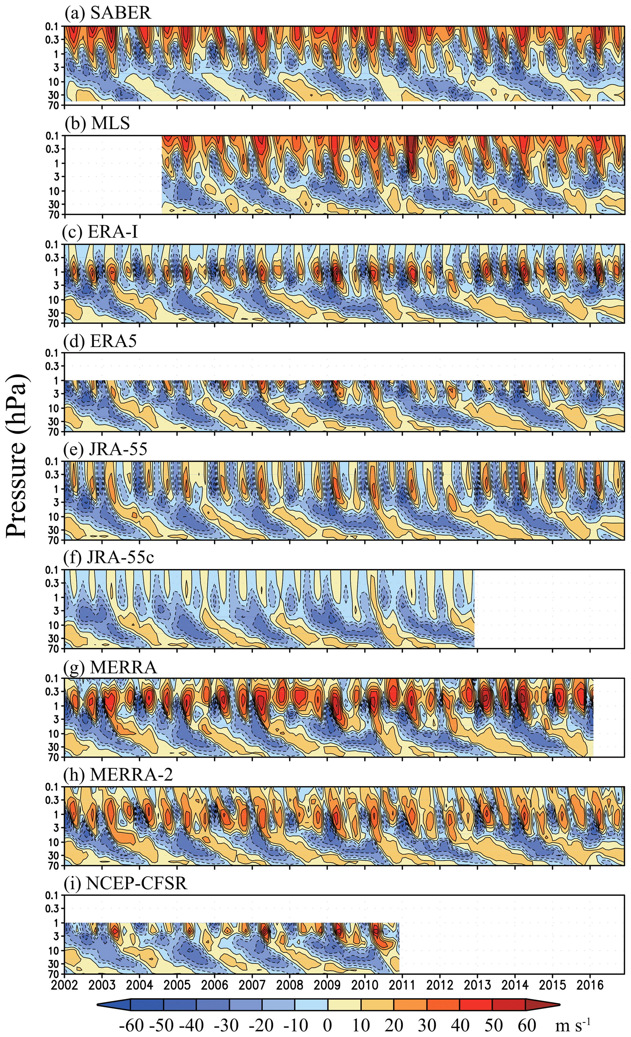
Figure 1 Time–height section of the equatorial zonal mean zonal wind in the (a) SABER and (b) MLS satellite-derived datasets as processed by Smith et al. (2017) and (c–i) each reanalysis from January 2002 to December 2016. The color intervals are 10 m s⁻¹.

Figure 2 displays vertical profiles of the climatological annual and zonal mean zonal wind and temperature over the Equator. Climatology is calculated from January 1980 to December 2010 for the reanalyses, whereas it is calculated for more recent years for the two satellite datasets after SABER and MLS data were available (from January 2002 and from January 2005, for SABER and MLS, respectively, until December 2016). For temperature, reanalyses agree well with the satellite climatology and differences among reanalyses are relatively small (the exception is JRA-55 above ∼0.5 hPa where it is an outlier, possibly due to the effects of the artificial sponge layer above 1 hPa). In contrast, the spread among the reanalyses is quite large for the equatorial zonal wind. MERRA-2 shows a westerly bias compared to other reanalyses and observation above 20 hPa. Above 10 hPa, differences among both reanalyses and anomalies from SABER and MLS become significantly larger. Above 1 hPa, zonal winds in ERA-I and JRA-55 are fairly weak and those in MERRA and MERRA-2 trend toward zero above ∼0.5 hPa, presumably due to effects of sponge layers, while satellite observations represent stronger climatological westerlies at 0.1–1 hPa. The long-term mean of the satellite zonal winds showing mean easterlies in the middle stratosphere and westerlies in the lower mesosphere is in good overall agreement with that computed from rocketsonde observations at low latitudes (Hitchman and Leovy, 1986). We also have drawn these vertical profiles using averages from January 2005 to December 2010 (i.e., years that are available in all reanalyses and two satellites) and confirmed the results are not significantly affected by the choice of periods.

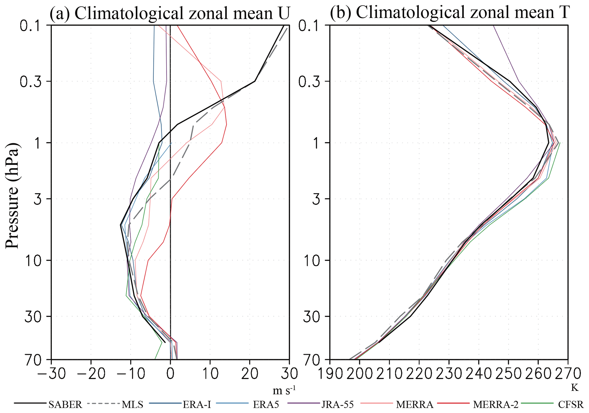
Figure 2 Vertical profiles of the climatological annual and zonal mean (a) zonal wind, and (b) temperature over the Equator for SABER (solid black), MLS (dashed black), ERA-I (blue), ERA5 (light blue), JRA-55 (purple), MERRA (pink), MERRA-2 (red), and NCEP-CFSR (green). Climatology is calculated from 1980 to 2010 in the reanalyses, from 2002 to 2016 in SABER, and from 2005 to 2016 in MLS.

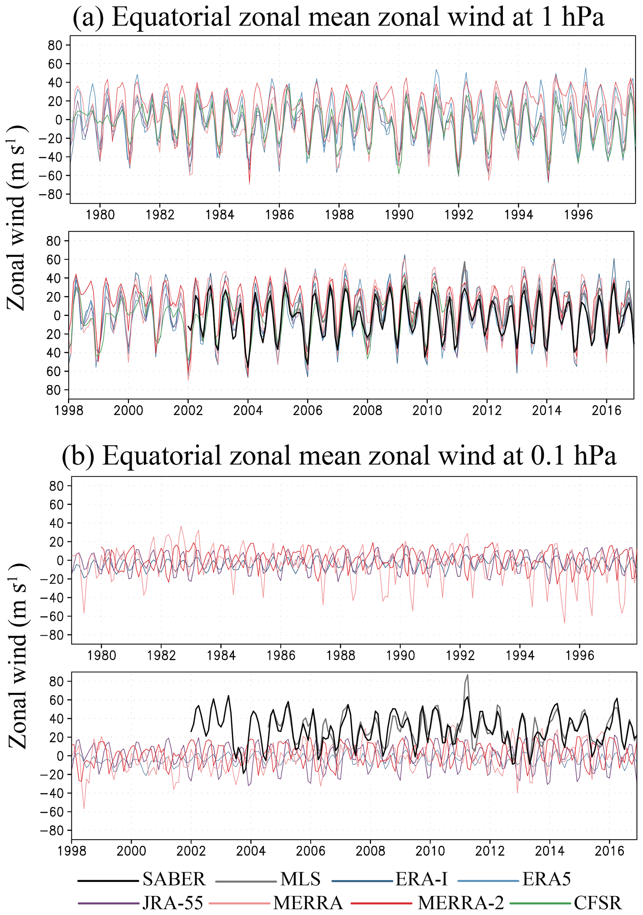
Figure 3 (a, b) Time variations of the equatorial zonal wind at (a) 1 hPa and (b) 0.1 hPa for SABER, MLS, and each reanalysis.

Figure 3 shows the time series of monthly mean zonal mean equatorial zonal wind in the satellite-derived datasets (black lines) and in each reanalysis. At 1 hPa, all reanalyses (ERA-I, ERA5, JRA-55, MERRA, MERRA2, and NCEP-CFSR) represent the SAO with qualitative agreement with the satellite-derived winds. However, there are substantial differences among the reanalyses in the individual months. MERRA-2 sometimes represents significantly stronger westerly extremes than other reanalyses (e.g., during 1980 and 1989). ERA-I and ERA5 also sometimes have stronger westerly extremes (e.g., in 1991 and 1996). At 0.1 hPa the disagreement among reanalyses (ERA-I, JRA-55, MERRA and MERRA-2) is larger. MERRA winds show much stronger easterlies than MERRA-2 until ∼1998, and these easterly extremes become smaller later on, as in MERRA-2, although the SAO phases between MERRAs are quite different (see also Fig. 9 shown later). At 0.1 hPa the winds derived from both the SABER and MLS satellite observations have a strong disagreement with all the reanalyses, which display much weaker westerlies in the annual, long-term mean (Fig. 2).

To quantify the spread among reanalyses, the standard deviation (SD) among the reanalyses is calculated as follows:

$$\begin{array}{}\text{(1)}& \text{SD}=\sqrt{\sum _i^N{\left(u_i-\left[u\right]\right)}^{\mathrm{2}}/N},\end{array}$$

where i represents the individual datasets from among the N datasets included. The square brackets [...] denote the mean over all N reanalyses. The SD is calculated for each month using the monthly mean zonal wind. We calculate the SD among all six reanalyses from 1980 to 2010, the SD among the five reanalyses (excluding NCEP-CFSR and extended until 2015), and the SD between the two MERRA versions (MERRA and MERRA-2) from 1980 to 2015. The SD among both six and five reanalyses is discussed up to 1 hPa, whereas the SD between MERRA and MERRA-2 is discussed up to 0.1 hPa (i.e., the maximum altitude of pressure data provided).

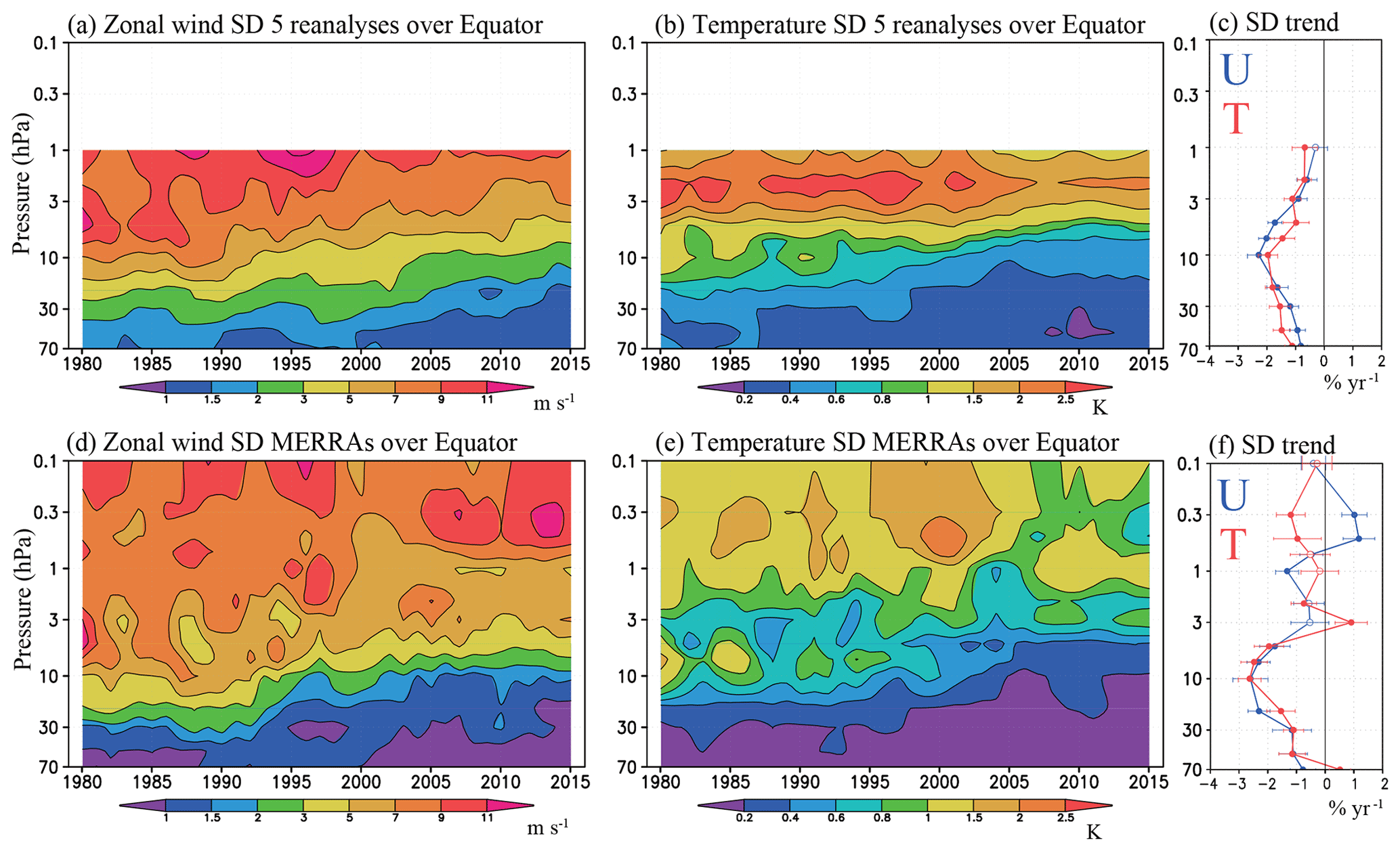
Figure 4 Time–height cross section of zonal mean annual mean standard deviation of (a, d) zonal wind and (b, e) temperature among (a, b) five reanalyses (ERA-I, ERA5, JRA-55, MERRA, MERRA-2) and (d, e) between MERRA and MERRA-2 over the Equator from 1980 to 2015. The 3-year running mean values are plotted in each case. The color intervals are 1, 1.5, 2, 3, 5, 7, 9, and 11 m s⁻¹ for zonal wind and 0.2, 0.4 0.6, 0.8, 1, 1.5, 2, and 2.5 K for temperature. (c, f) The linear regression trends in the standard deviation (in percent per year) over time with height in (blue) zonal wind and (red) temperature (c) among five reanalyses and (f) between MERRAs. Filled circles indicate that the trend at that level is different from zero with a statistical significance P<0.05. Error bars denote P<0.05 confidence intervals in the trend estimates.

The time–height section of the zonal mean SD of the equatorial zonal wind and temperature among the five reanalyses and only between MERRA and MERRA-2 is shown in Fig. 4. Three-year running mean of annual mean SD is performed on the SD. Figure 4c and f show the linear regression trend in the SD at each level over the whole record. Trends are expressed in terms of percentage per year at each level (note that linear trends are not always appropriate in this case, as the SD sometimes drops with the introduction of new observational data in the assimilation, as shown in Kawatani et al., 2016).

Both zonal wind and temperature SDs among five reanalyses decrease with time, a trend that is particularly clear at levels from 70 to ∼2 hPa. As discussed in Kawatani et al. (2016), one possible reason for the reduction of the SD over time is the upgrading of satellite radiance observations. From 1979 to 2006, the Television InfraRed Operational Satellite (TIROS) Operational Vertical Sounder (TOV), Stratospheric Sounding Unit (SSU), and Microwave Sounding Unit (MSU) were available. After May 1998, data from the Advanced Microwave Sounding Unit (AMSU) became available. Satellite radiance data will presumably affect the assimilated temperatures in the stratosphere but will also have considerable influence on the wind (see Iida et al., 2014). Near the Equator thermal wind shears are particularly sensitive to small errors in observed temperatures. After 2000, the amount of available satellite data increased greatly (e.g., Kobayashi et al., 2015), and the contributions of satellite radiance data to better representation of the tropical winds also presumably increased. Kawatani et al. (2016) also showed the evolution of the number of available monthly mean near-equatorial radiosonde observations at 10–70 hPa. The number of available radiosonde observations generally increased with time at all levels, which also likely contributed to the decreasing trend of SD among reanalyses from 70 to 10 hPa. The SDs between MERRAs show a similar decrease with time, although time variations of both zonal wind and temperature SDs above 1 hPa are more complicated.

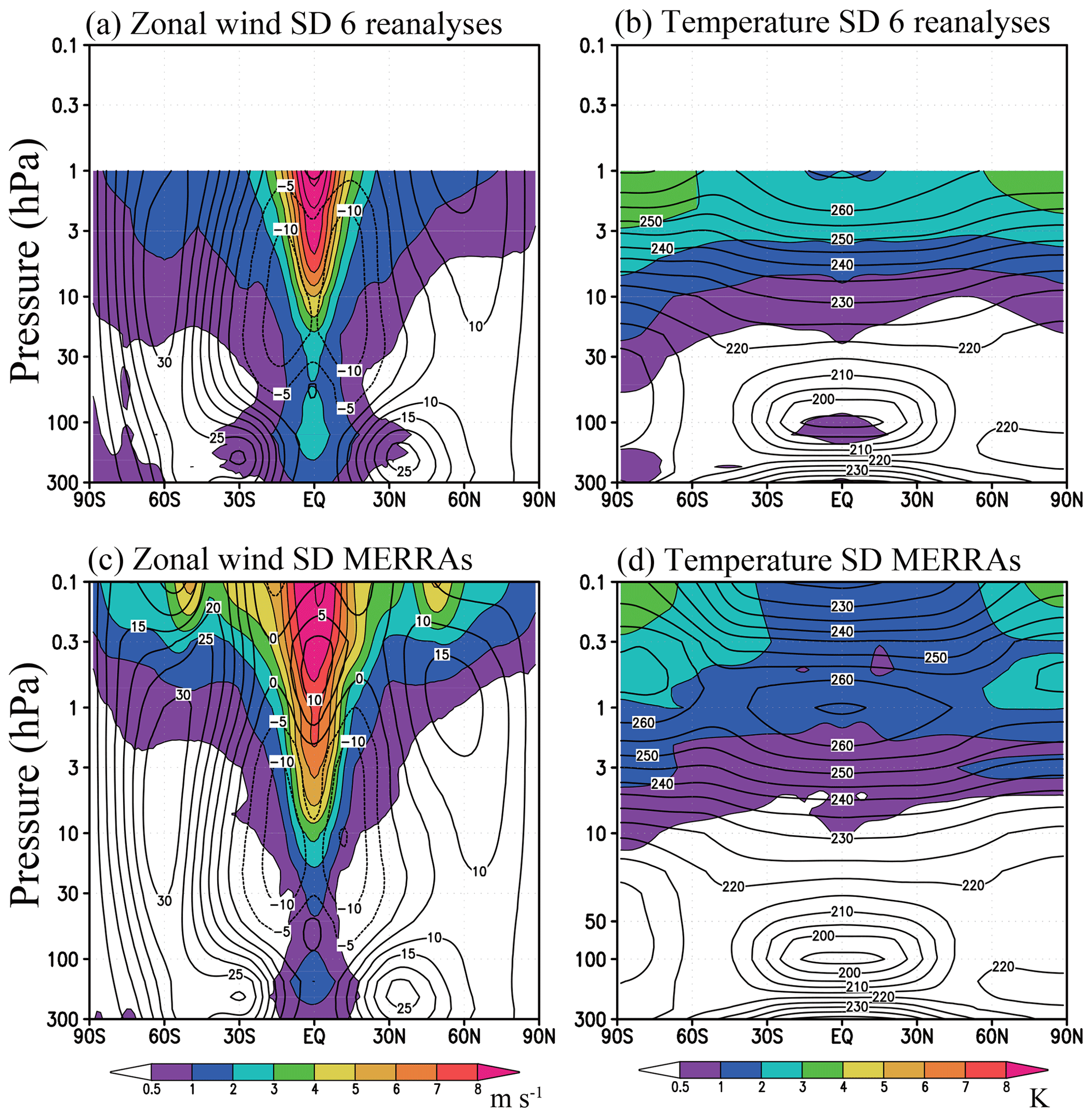
Figure 5 Latitude–height cross sections of climatological zonal mean standard deviation of (a, c) zonal wind and (b, d) temperature (a, b) among six reanalyses and (c, d) between MERRA and MERRA-2. The color intervals are 0.5, 1, 2, 3, 4, 5, 6, 7, 8 m s⁻¹ and K for zonal wind and temperature, respectively. Shading indicates values larger than 0.5 m s⁻¹ and 0.5 K.

Next, we explore spatial variation of SD among reanalyses. Figure 5 displays the latitude–height distributions of the zonal means of the zonal wind and temperature SD among six reanalyses averaged from 1980 to 2010, as well as the SD between MERRA and MERRA-2. In the SD among the six reanalyses (Fig. 5a and b), the largest values are on the Equator and increase from the upper troposphere to the upper stratosphere so that the largest values occupy a wedge-shaped region shown clearly in the Fig. 5. The temperature SD shows an opposite structure, having a minimum SD in the lower latitudes and becoming larger at higher latitudes. Near the Equator small differences in temperature (say between two reanalysis datasets) can be expected to result in large differences in the thermal wind shear. The zonal wind and temperature SDs between MERRA and MERRA-2 (Fig. 5c and d) show qualitatively similar structures. The local maxima of zonal wind SD around 50^∘ S and 50^∘ N at 0.1–0.3 hPa arise from the different shape of the mesospheric jets between MERRA and MERRA-2 (not shown). This may result from the inclusion of parameterized non-orographic gravity wave drag in MERRA-2. The observational constraints in the lower mesosphere are much weaker and the representation of the zonal winds may depend strongly on the model configuration used in each reanalysis.

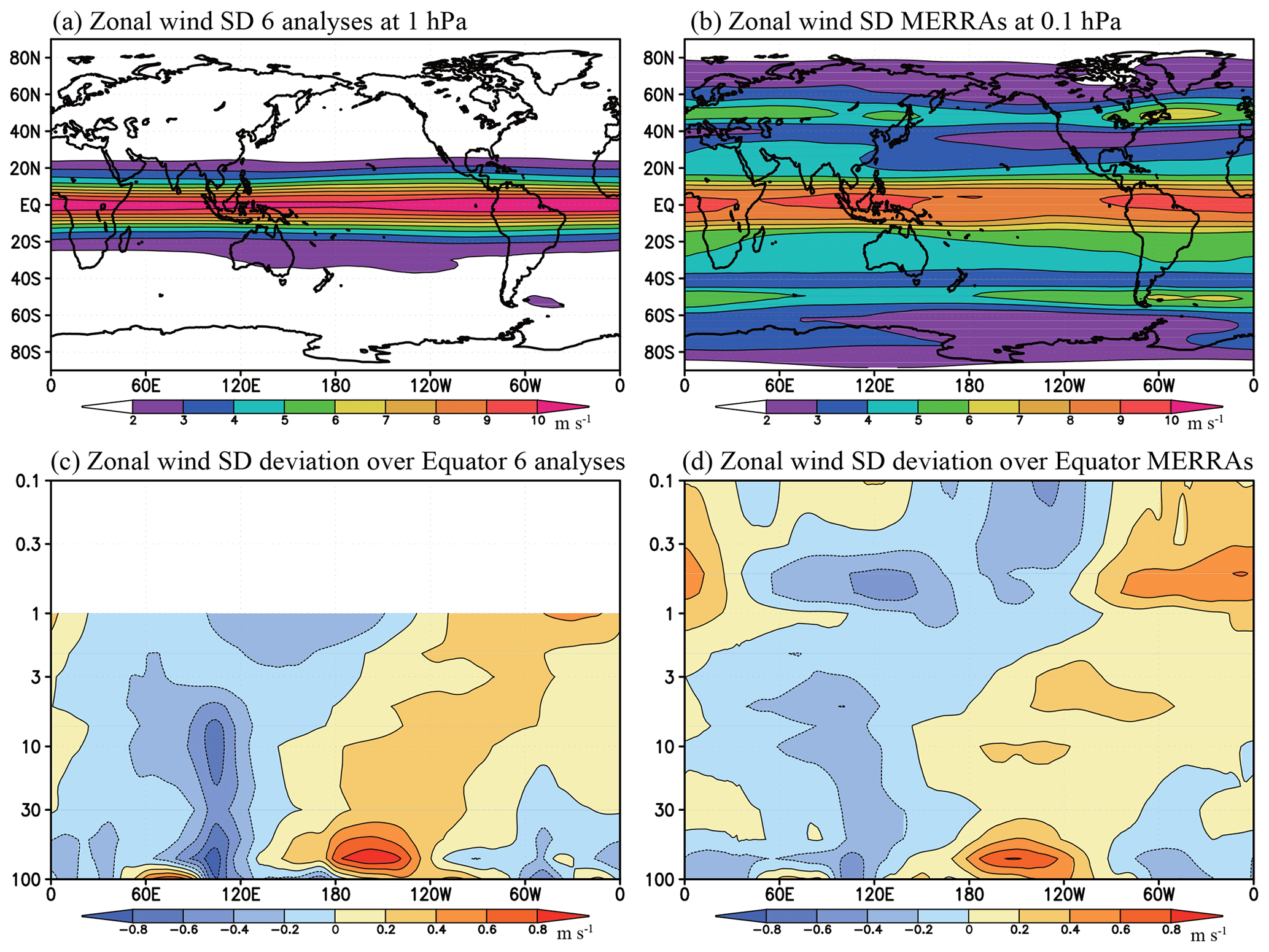
Figure 6 (a, b) Horizontal maps of climatological zonal wind standard deviation (a) among the six reanalyses at 1 hPa and (b) between MERRA and MERRA-2 at 0.1 hPa. (c, d) Longitude–height cross section of the anomaly of the zonal wind standard deviation from its zonal mean over the Equator (c) among the six reanalyses and (d) between MERRA and MERRA-2. The color intervals are 1 m s⁻¹ for (a, b) and 0.2 m s⁻¹ for (c, d).

Figure 6a shows the horizontal distributions of the zonal wind SD among six reanalyses at 1 hPa. The SD shows a fairly zonally uniform structure. Kawatani et al. (2016) showed the zonal wind SD from 70 to 10 hPa, and noted that the SD becomes more zonally uniform as height increases. The 0.1 hPa SD between the MERRAs also shows a fairly zonally uniform structure (Fig. 6b). Figure 6c and d display the longitude–height cross section of zonal wind SD after the zonal mean of the SD is subtracted. This shows that there actually are some systematic zonal variations in the SD. Notably positive SD anomalies are found in the central Pacific,in the lower to middle stratosphere, where in situ observations are few (Fig. 5 of Kawatani et al., 2016). The smallest SD is seen near Singapore (1.4^∘ N, 104^∘ E), where high-quality radiosonde observations up to 10 hPa are consistently available (Naujokat, 1986). It is interesting that the region of reduced SD (negative SD anomaly in Fig. 5c) extends up to ∼3 hPa. This suggests that the influence of in situ observations near the Equator on the reanalyses extends to altitudes considerably above the actual observation heights. At 1 hPa, the SD in the Eastern Hemisphere is slightly smaller than that in the Western Hemisphere. Another region of small SD over South America around 50^∘ W does not extend as high as it does over the Singapore, because the observational density at 10 hPa is significantly lower over South America, and the higher density is limited at 50–70 hPa (Fig. 5 in Kawatani et al., 2016). The zonal wind SD between MERRA and MERRA-2 (Fig. 6b and d) also show a similar structure; however, the reason for the sudden increase of the zonal asymmetry of the SD at ∼0.5 hPa is unclear.

4 Similarities and differences of the semiannual oscillation among the reanalyses

In this section, we focus on the similarities and differences of the seasonal cycle (dominated of course at low latitudes by the semiannual component) among reanalyses. Figure 7a shows the long-term mean annual cycle of zonal mean equatorial zonal wind at 1 hPa, as derived from SABER and MLS observations and in each reanalysis. Some differences are seen between the winds based on SABER and MLS, e.g., stronger westerly maxima (around April and October) and weaker easterly maxima (around January and July) in the MLS-derived winds compared to the SABER-derived winds (also consistent with the long-term annual mean equatorial zonal wind shown in Fig. 2a). The reanalysis zonal winds shown in Fig. 7a in most months are within ∼10 m s⁻¹ of one of the satellite-derived values, with the exception of MERRA-2, which has clear westerly biases in all months compared to satellite-derived winds and actually displays westerlies for the climatological values in July (i.e., during the second easterly phase of the SAO, as shown in other datasets).

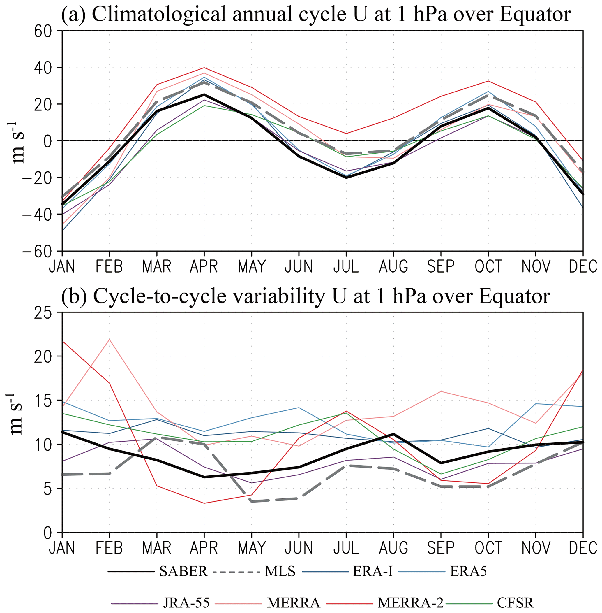
Figure 7 (a) Climatological mean annual cycle of zonal mean zonal wind over the Equator at 1 hPa for SABER, MLS, and each reanalysis; (b) cycle-to-cycle variability of equatorial zonal mean zonal wind calculated as the interannual standard deviation in each calendar month. Climatology and standard deviation are calculated from 1980 to 2010 in the reanalyses, from 2002 to 2016 in SABER, and from 2005 to 2016 in MLS.

Figure 7b shows a measure of the interannual variability of equatorial zonal mean zonal wind in observations and reanalysis. This variability is characterized by the SD for each calendar month. For example, January SD in each reanalysis is calculated from the monthly mean zonal wind data from 1980 to 2010 (31 data points). Note that the analyzed periods for the satellite-derived winds are shorter than those of the reanalyses (after January 2002 and 2005 for MLS and SABER, respectively, until December 2016); reanalyses generally have a larger SD compared to satellite-derived winds. The SD in MERRA-2 varies significantly among months, being larger during the easterly phase of the SAO than during the westerly phase. The interannual SD of ERA-I, ERA5, JRA-55, and NCEP-CFSR show little variability through the year, as do the satellite-derived winds from both SABER and MLS.

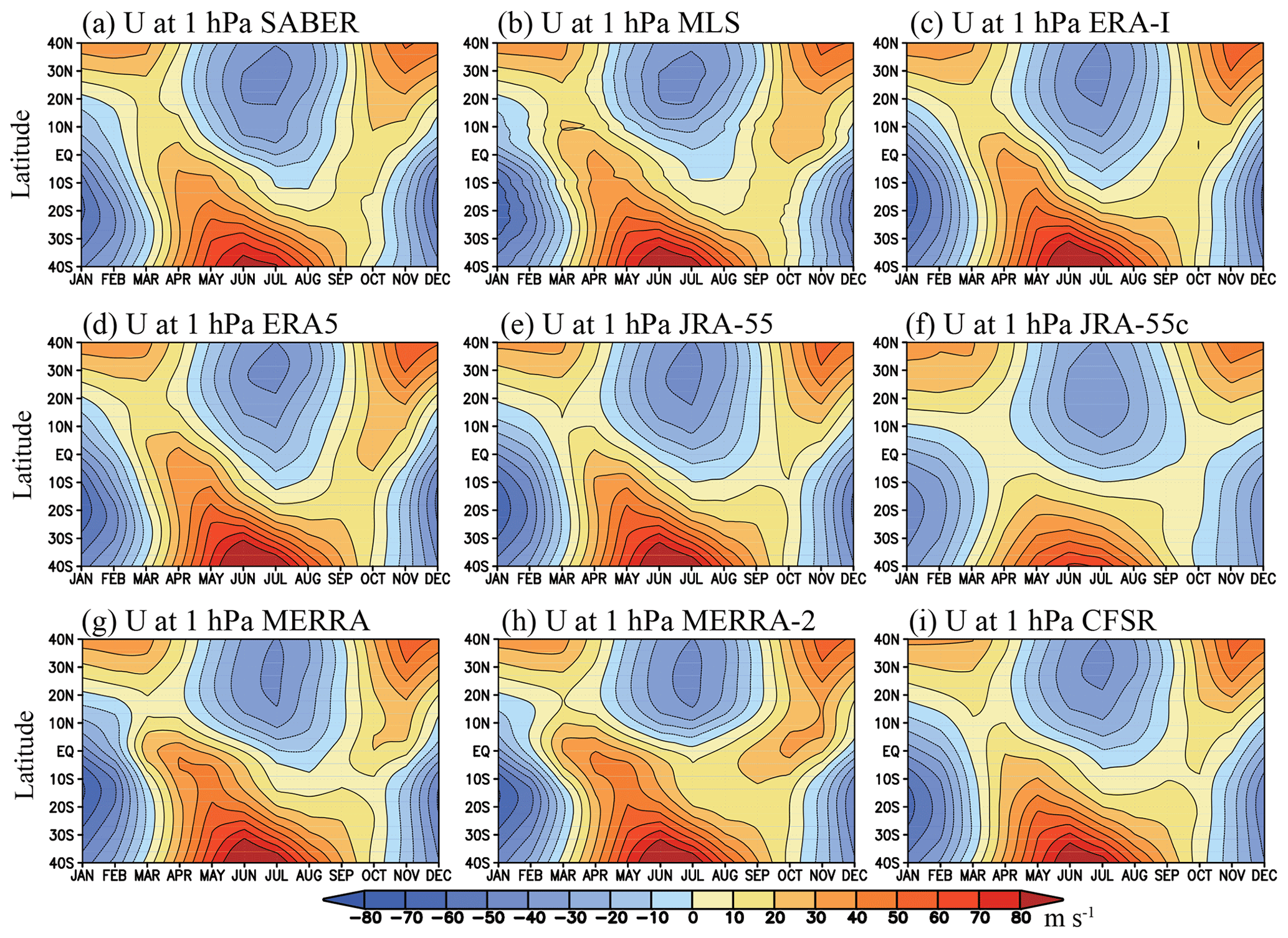
Figure 8 Time–latitude sections of climatological mean annual cycle of the zonal mean zonal wind for (a) SABER, (b) MLS, and (c–i) each reanalysis at 1 hPa. The contour intervals are 10 m s⁻¹. Climatology is calculated from 1980 to 2010 in the reanalyses, from 2002 to 2016 in SABER, and from 2005 to 2016 in MLS.

Figure 8 shows the time–latitude cross sections of the climatological annual cycle of the zonal mean zonal wind at 1 hPa for individual datasets (in the rest of this section, results of JRA-55C are included again to compare it to JRA-55). The patterns are similar between satellite-derived winds based on MLS and SABER, as already shown in Smith et al. (2017, their Fig. 5). The easterlies extend into the tropics from the summer hemisphere during the solstices; the westerlies exist at all latitudes during the equinox season. This characteristic is qualitatively represented by all reanalyses. MERRA-2 features significantly stronger equatorial westerlies around both equinoxes. This can be explained by the fact that the westerly phase of the SAO is believed to be driven mainly by the atmospheric waves (Dunkerton, 1982), and the dynamical model used in MERRA-2 includes quite strong parameterized momentum fluxes from non-orographic gravity waves (Fig. 3 of Molod et al., 2015). In contrast, JRA-55 and NCEP-CFSR represent weaker westerlies during equinoxes. Comparing JRA-55 to JRA-55C, both easterlies and westerlies are significantly weaker in JRA-55C, once again demonstrating the significant contribution of satellite temperature observations to the representation of a realistically strong SAO.

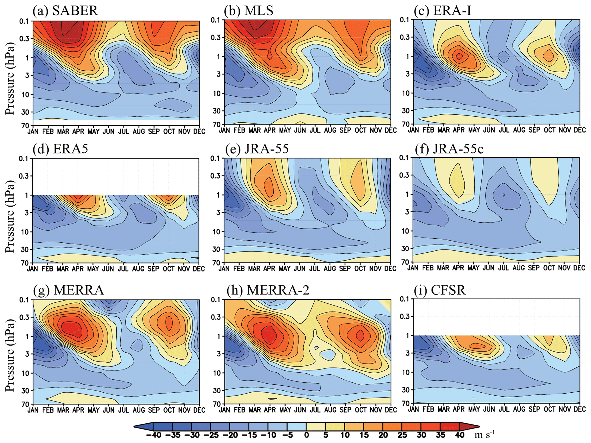
Figure 9 Time–height sections of climatological mean annual cycle of the zonal mean zonal wind over the Equator for (a) SABER, (b) MLS, and (c–i) each reanalysis. Climatology is calculated from 1980 to 2010 in the reanalyses, from 2002 to 2016 in SABER, and from 2005 to 2016 in MLS. The contour intervals are 5 m s⁻¹.

Figure 9 shows time–height cross sections of the climatological mean annual cycle of the zonal mean zonal wind over the Equator in each of the datasets. The satellite-derived winds from SABER and MLS (Fig. 9a and b) agree fairly well, particularly below about 0.3 hPa and these results agree reasonably well with the time–height section of the SAO determined from rocketsonde observations (Garcia et al., 1997; Smith et al., 2017). The equinoctial maxima of the westerly peaks are above 0.1 hPa, while the easterly wind peaks are at ∼1 hPa. The satellite-derived winds clearly show that the SAO cycle in the first half of the year (boreal winter and spring) is stronger than that in the second half (austral winter and spring), a feature that has been apparent since the earliest rocketsonde studies of the SAO (Reed, 1966). All of the reanalysis zonal wind datasets differ considerably from the satellite-derived winds, and the reanalyses differ significantly among themselves as well. The SAO descending westerlies in the SABER- and MLS-derived data penetrate down to ∼5–7 hPa in the first cycle of the year and ∼3 hPa in the second cycle. The westerlies do not penetrate quite as far down in ERA-I, ERA5, JRA-55, JRA-55C, and NCEP-CFSR. This westerly penetration seen in the satellite data is reasonably well represented in MERRA, while MERRA-2 displays an even further downward penetration of the westerlies. MERRA-2 is also the only dataset considered that does not display easterly mean winds at 1 hPa in July and August.

At 0.1 hPa, both the SABER- and MLS-derived equatorial zonal winds (Fig. 9a and b) are westerly throughout the year, while both MERRA and MERRA-2 show easterly phases, although the timing of easterly appearance is different (December and June for MERRA and April and October for MERRA-2). ERA5 data above 1 hPa are not currently available publicly, but Shepherd et al. (2018) did have access to ERA5 at higher levels for the period 2008–2017, and they note that ERA5 has westerlies throughout the year in the long-term mean wind field at 0.1 hPa averaged over 5^∘ S–5^∘ N, which is more similar to the SABER- and MLS-derived winds and very different from ERA-I (Fig. 9c).

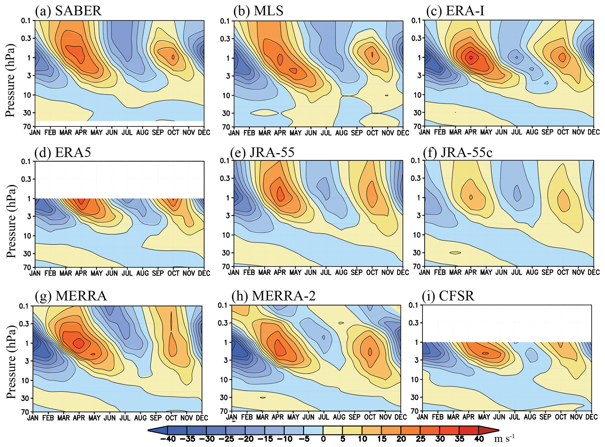
Figure 10 The same as Fig. 9 but with annual mean climatological zonal winds (shown in Fig. 2a) removed at each level.

Figure 10 is the same as Fig. 9, except that long-term annual mean climatology (i.e., the mean zonal wind in Fig. 2a) has been removed at each level. In this figure, the SAO easterly and westerly phases are more clearly visible. A stronger SAO easterly in the first cycle compared to the second cycle is seen in both observations and all reanalyses. Differences among reanalyses are still obvious in this figure.

To investigate the SAO in more detail, SAO components were extracted from each of the datasets considered here and then the SAO amplitude was calculated as follows:

$$\begin{array}{}\text{(2)}& \text{SAO amplitude}=\sqrt{\mathrm{2}}\times \sqrt{\sum _i^N{u_i^{\prime }}^{\mathrm{2}}/N},\end{array}$$

where u^′ is the monthly mean zonal wind of the filtered SAO component, and the sum is over all the months in the time series for each dataset.

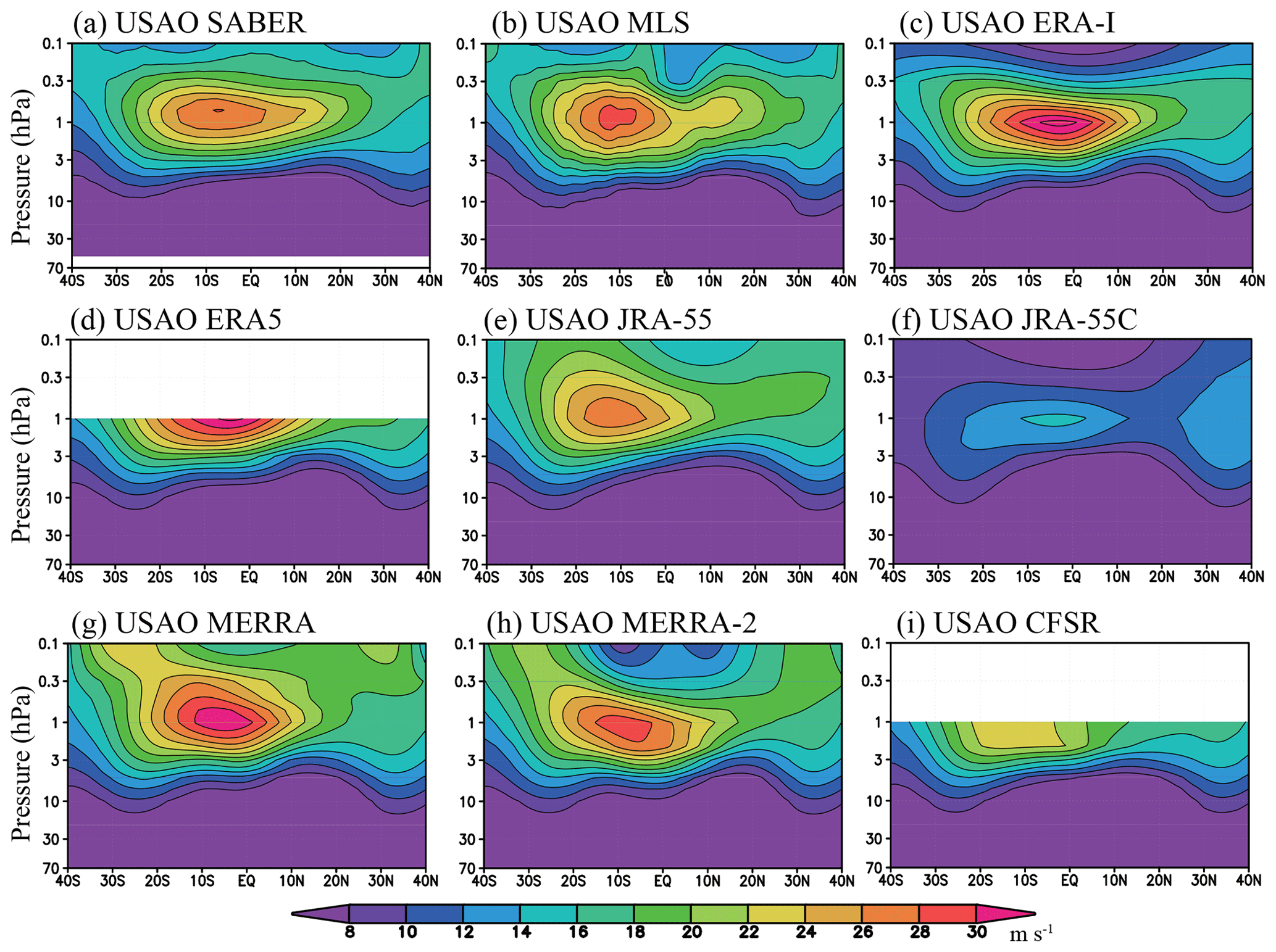
Figure 11 Latitude–height cross section of amplitude of the SAO in zonal wind. Color intervals are 2 m s⁻¹. The amplitude is calculated from 1980 to 2010 in the reanalyses, from 2002 to 2016 in SABER, and from 2005 to 2016 in MLS.

Figure 11 shows the latitude–height cross section of SAO amplitude in zonal wind. The observed SAO amplitude has its maximum off the Equator in the Southern Hemisphere, around 7.5^∘ S in the SABER-derived dataset and 12^∘ S in the MLS-derived dataset. These results are in basic agreement with the earlier study of Hopkins (1975), who analyzed the SAO amplitude determined from roughly 10 years of rocketsonde data at several stations and concluded that the SAO amplitude near the stratopause peaked around 10–15^∘ S. The SAO amplitude from the MLS-derived winds has a more pronounced asymmetry between the Northern Hemisphere and Southern Hemisphere, notably with the region of large amplitude near the stratopause appearing thinner on the northern side of the Equator, again reminiscent of the pattern in the Hopkins (1975) result. Note again that the near-equatorial winds in our satellite-derived datasets were estimated by cubic spline interpolation of the balance winds at and poleward of latitude $\pm \mathrm{8}{}^{\circ }$ for SABER and $\pm \mathrm{6}{}^{\circ }$ for MLS (Smith et al., 2017) and that this must introduce uncertainty in the wind estimates near the Equator in each case.

The results for the SAO zonal wind amplitude for each of the reanalyses (Fig. 11c–i) show the overall pattern of a peak near the low-latitude stratopause, but the details differ quite substantially among the different datasets. Notably, the degree of interhemispheric asymmetry differs: the maximum latitude of the SAO amplitude at 1 hPa is at 3^∘ S in ERA-I, 4.5^∘ S in ERA5, 12^∘ S in JRA-55, 3^∘ S in JRA-55C, 4.5^∘ S in MERRA, 9.5^∘ S in MERRA-2, and 13.5^∘ S in NCEP-CFSR. The peak SAO wind amplitude is larger than in the satellite-derived datasets (Fig. 11a and b) in ERA-I, ERA5, and MERRA but smaller in NCEP-CFSR. The SAO peak amplitude is much weaker and occurs at a lower altitude in the JRA-55C vs. the JRA-55 reanalyses. Poleward of 20^∘ in both hemispheres, the SAO amplitude becomes larger with latitude (e.g., from 20^∘ S to 30^∘ S and/or 20^∘ to 30^∘ N, from 0.3 to 1 hPa) in both MERRA and MERRA-2 (Fig. 11g and h), features that find no support in the corresponding result from the satellite-derived datasets (Fig. 11a and b).

Figure 12 The same as Fig. 11 but for the SAO in temperature. Color intervals are 0.4 K.

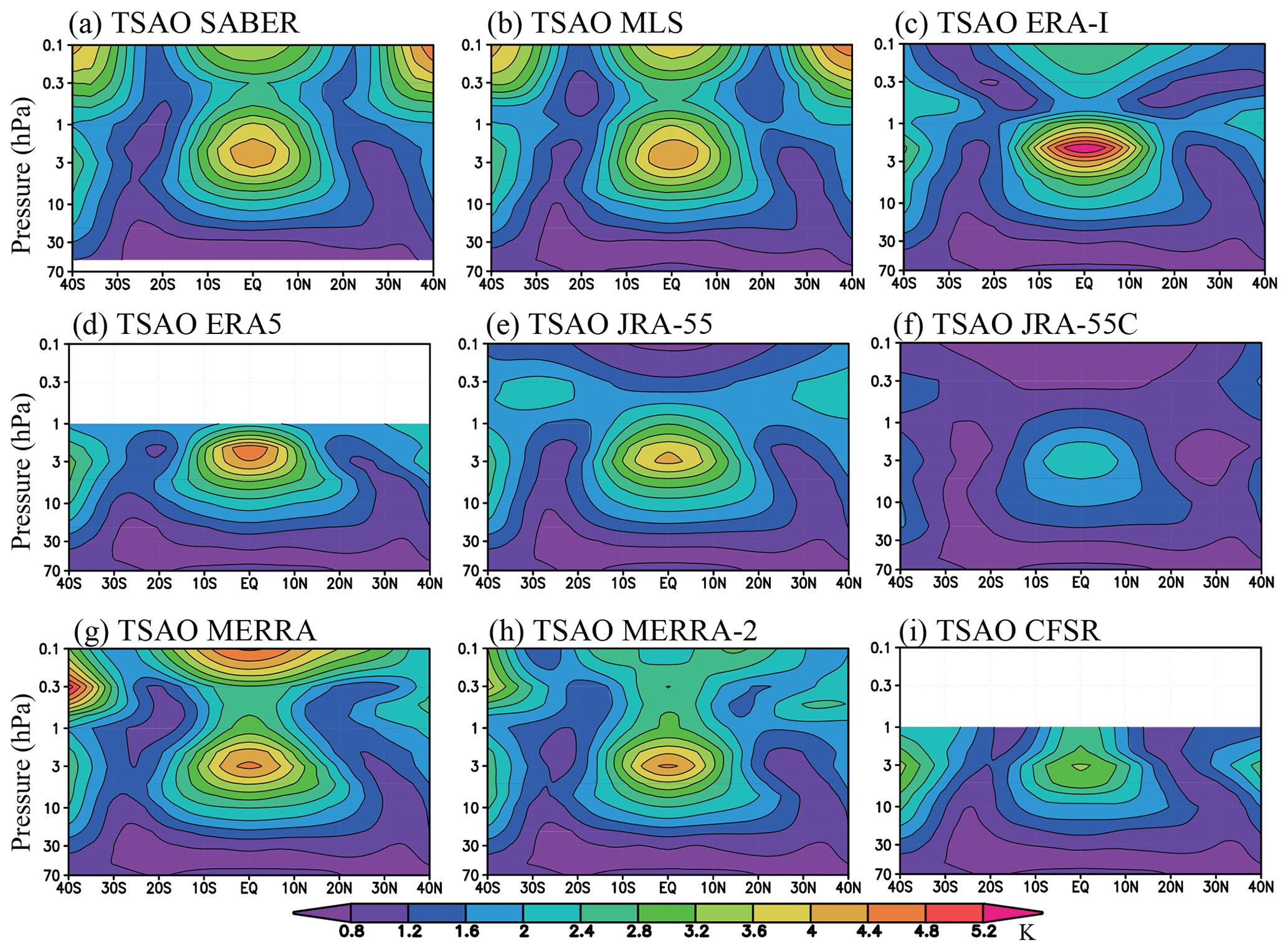
Figure 12 shows the same amplitude estimate as in Fig. 11, but for the SAO in temperature. In contrast to the zonal wind, the temperature SAO amplitude is equatorially centered and appears to be distributed more symmetrically about the Equator. Different latitudinal gradients of the temperature, which are larger in the Southern Hemisphere, result in a southward shift of the maximum zonal wind amplitude in the satellite-derived datasets. The maximum SAO amplitude of temperature over the Equator is found at 2–3 hPa, with another peak at 0.1 hPa in both SABER and MLS. Large SAO components are also found at 40^∘ S and 40^∘ N at 0.1 hPa in both the SABER and MLS observations.

The temperature SAO amplitude at 2 hPa over the Equator is approximately 4.3 K (SABER), 4.2 K (MLS), 5.6 K (ERA-I), 4.7 K (ERA5), 4.0 K (JRA-55), 2.2 K (JRA-55C), 4.2 K (MERRA), 3.9 K (MERRA-2), and 2.9 K (NCEP-CFSR). ERA-I and ERA5 overestimated the temperature SAO amplitude compared to the satellite observations, while the amplitude is significantly underestimated in NCEP-CFSR. The much weaker SAO apparent in JRA-55C than JRA-55 (Fig. 11f vs. Fig. 11e) again demonstrates the key role assimilated satellite data play in defining the SAO in reanalyses. For the second amplitude maximum over the Equator at 0.1 hPa, MERRA has a larger peak value and meridionally wider structure compared with the amplitude computed from the satellite datasets, while MERRA-2 significantly underestimates this maximum. The 0.1 hPa equatorial maximum seen in the satellite datasets is not apparent in the JRA-55 reanalyses and is quite weak in the ERA-I reanalyses. These discrepancies may be attributable to the sponge layers with strong numerical dumping of wave components above 1 hPa for ERA-I and JRA-55. The large SAO amplitudes near 0.1 and 40^∘ S and 40^∘ N have no counterpart in any of the reanalysis datasets except possibly MERRA and MERRA-2 near 40^∘ S.

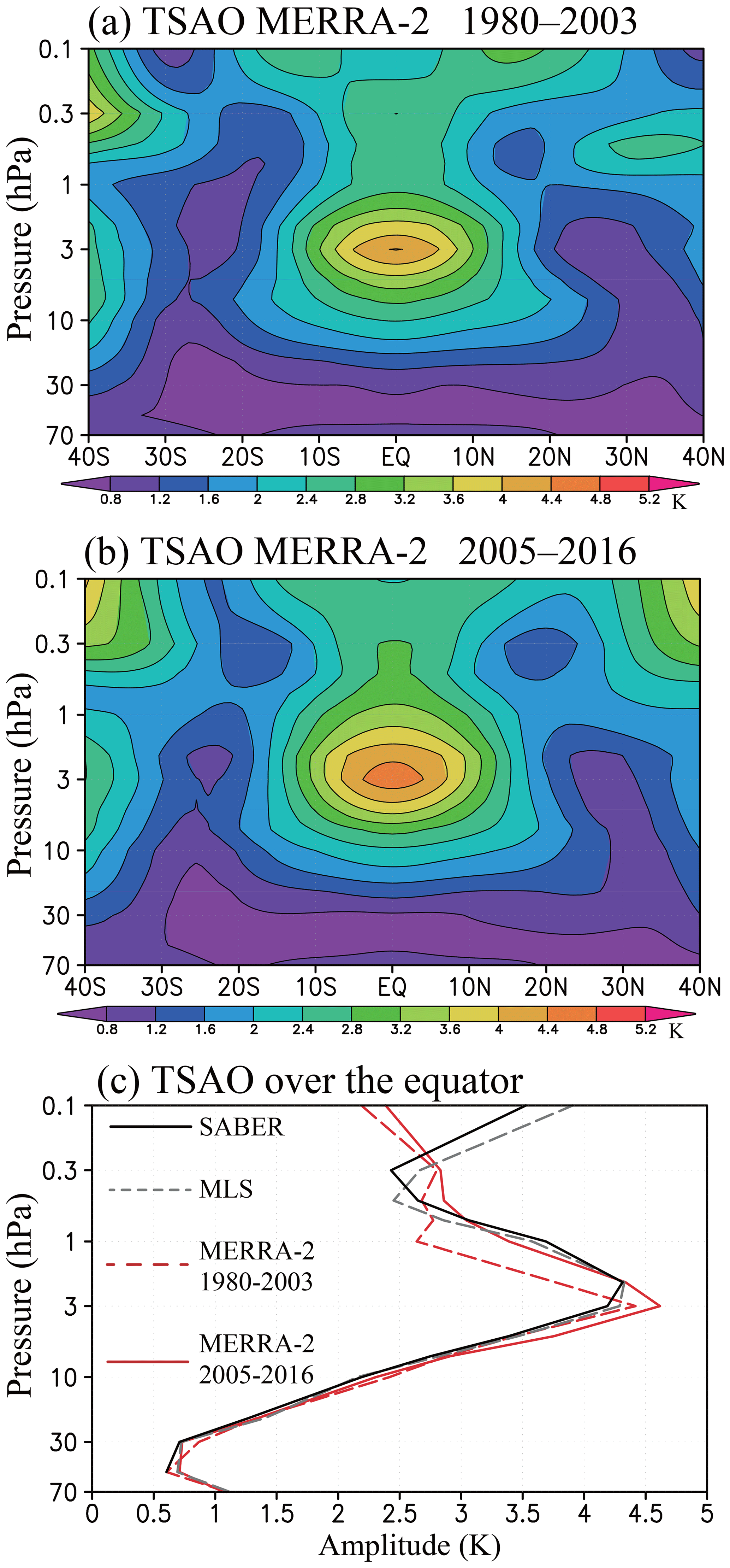
Figure 13 (a, b) Latitude–height cross section of SAO temperature amplitude for MERRA from (a) 1980 to 2003 and (b) 2005 to 2016. (c) Vertical profiles of SAO temperature amplitude over the Equator for SABER (solid black), MLS (dashed black), MERRA-2 from 1980–2003 (dashed red), and MERRA-2 from 2005 to 2016 (solid red).

The amplitudes shown for the reanalysis datasets in Fig. 12 are calculated using all the data from January 1980 to December 2010. Here, it should be noted that MERRA-2 is the only reanalysis that assimilates the MLS temperature above 5 hPa. Thus, some improvement is expected for MERRA-2 in the SAO temperature field after the MLS data were assimilated starting in August 2004. Figure 13a and b shows the same quantity as Fig. 12 but for MERRA-2 in 1980–2003 (i.e., pre-MLS years) and in 2005–2016 (i.e., when the MLS data are included in the assimilation over each entire year). Figure 13c shows vertical profiles of the temperature SAO amplitude over the Equator for SABER, MLS, and MERRA-2 in 1980–2003 and in 2005–2016. It is evident that over ∼2–0.5 hPa the MERRA-2 SAO amplitude over the Equator became closer to the SABER and MLS observations after the MLS temperature was assimilated, although the significantly smaller amplitude at 0.1 hPa is not improved. Notably, the MERRA-2 representation of the SAO amplitude near 0.1 hPa and 40^∘ S and 40^∘ N improves in the period with MLS data included in the assimilation.

5 Summary and concluding remarks

The systematic observation of the equatorial middle atmosphere began with balloon-borne radiosondes in the 1950s, rocketsondes and radars in the 1960s, and satellite radiance measurements in the late 1970s. These observations turned up interesting and unexpected phenomena, notably the occurrence of well-defined, very low-frequency oscillations of the zonal mean circulation at various altitudes: the QBO in the lower and middle stratosphere and the SAO with large amplitude in the stratopause region and then again in the mesopause region. The tropical middle atmosphere has its own unique dynamics and is known to be particularly challenging for realistic simulation by comprehensive general circulation models (e.g., Butchart et al., 2018). Global reanalyses have proven to be very valuable in efforts to understand the dynamics of the atmosphere and the climate system, but the accurate representation of the atmospheric flow in gridded analyses is particularly challenging for the tropical middle atmosphere. As discussed in the introduction of Kawatani et al. (2016), the initial attempts in the 1980s and 1990s at global analyses based on variational assimilation into dynamical model integrations produced results with very poor representation of the tropical stratosphere. More modern reanalysis datasets have produced much more satisfactory results, at least in the lower and middle stratosphere where a quite realistic QBO is apparent in the analyzed zonal wind and temperature fields. Kawatani et al. (2016) compared the monthly mean zonal wind field up to 10 hPa in several reanalysis datasets and found that the disagreement among the reanalyses was largest on the Equator and grew with height (at least up to 10 hPa).

In the present paper we assessed the representation of the zonal wind and temperature fields near the Equator in the region 10–0.1 hPa, where the dominant feature is the near-stratopause SAO. One complication of examining this region is the nearly complete lack of relevant in situ measurements to compare with. While the SAO was first discovered in rocketsonde wind measurements, Baldwin and Gray (2005) found that rocketsonde data at stations within 10^∘ of the Equator that were frequent enough to produce reasonable monthly mean zonal winds were only available from 1965 to 1983. There is very little overlap with the reanalysis datasets we evaluated, as our interest is confined to reanalyses after 1979 when satellite radiometer data are included in the assimilations. In our project we compared, where possible, the reanalyses to observed limb-sounding radiometer data from SABER and MLS, using both the temperature retrievals and the analysis of Smith et al. (2017), who applied a dynamical balance relation to compute zonal winds from the geopotentials derived from the SABER and MLS temperatures.

Our study evaluated six major global atmospheric reanalysis datasets that have been widely applied in studies of the middle atmosphere (ERA-I, ERA5, JRA-55, MERRA, MERRA-2, and NCEP-CFSR). All six reanalyses have a good representation of the QBO in the equatorial lower and middle stratosphere, and each displays a clear SAO centered near the stratopause. However, the differences among reanalyses are much more substantial in the SAO region than in the QBO-dominated lower and middle stratosphere. We followed Kawatani et al. (2016) in characterizing the degree of disagreement among the reanalyses using the SD of the monthly mean zonal wind and temperature. The zonal wind SD has an equatorial maximum that increases with height. Above 10 hPa even the long-term annual mean equatorial wind differs substantially among the reanalyses. Above 10 hPa there are also substantial differences in the equatorial zonal wind fields between each of the reanalyses and the two satellite-derived wind datasets.

In their study of low-latitude winds below 10 hPa, Kawatani et al. (2016) found substantial zonal variation in the SD characterizing the disagreement among reanalyses. Notably, this was tied to the availability of in situ balloon measurements: the smallest SD was around the longitude of Singapore, where consistently high-quality near-equatorial radiosonde observations are available, and the largest values were around the eastern and central Pacific, where there are virtually no stratospheric in situ wind observations close to the Equator. Kawatani et al. (2016) found that the zonal contrast is reduced as height increases, but that a significant variation is still found at 10 hPa. In the present study, we extended this analysis to the 0.1 hPa level. Interestingly the near-Singapore minimum in SD is evident to at least ∼3 hPa (Fig. 6), i.e., considerably higher than the usual ∼10 hPa ceiling for weather balloons.

Over the Equator we showed that there are overall long-term trends for both the zonal wind and temperature SD to become smaller and this is seen clearly from 70 to ∼2 hPa (Fig. 4). Since within each reanalysis the dynamical atmospheric model and the analysis procedures are fixed, improvement with time must be related to an increase or improvement in the actual observations available for assimilation. The temperature sounders on NOAA operational satellites were upgraded significantly in May 1998, from the SSU to the Advanced Microwave Sounding Unit (AMSU). Kawatani et al. (2016) showed an improvement around 1998 of the QBO representation up to 10 hPa and a reduction in the wind and temperature SD. The present paper shows that the long-term decreasing trend of the SD is seen up to at least ∼2 hPa.

The latitude–height cross sections of the SD display opposite structures between zonal wind and temperature (Fig. 5). The zonal wind SD has a prominent equatorial maximum, indicating the particularly challenging nature of the reanalysis problem in the low-latitude stratosphere, where the Coriolis parameter is small and in situ observations are sparse. The zonal wind SD in low latitudes becomes larger with height, showing a wedge-shaped structure. In the mid-to-high latitudes, the zonal wind SD becomes smaller. In contrast, the temperature SD has minimum values over the Equator and maximum values in the polar region, which might be related to the observational density (i.e., significantly fewer observations in the polar regions).

We also examined the representation of the upper stratospheric winds and temperatures off the Equator. All of the reanalyses represent features of the time–latitude variation of the zonal mean zonal wind at 1 hPa that agree broadly with the satellite-derived datasets (Fig. 8). Notably, westerlies are present at all latitudes during the equinox seasons, while easterlies are clear in the summer hemisphere and extend to the Equator around the solstices. In addition, the amplitude of the SAO in wind and temperature as a function of height and latitude was computed from each dataset (Figs. 11 and 12). The zonal wind SAO amplitude in each case shows a maximum near 1 hPa and at low latitudes, but the details vary somewhat from dataset to dataset. All the results show that the peak SAO is displaced off the Equator somewhat into the Southern Hemisphere (in agreement with earlier studies using rocketsonde measurements), but the extent of the displacement and the values of the peak SAO amplitude vary considerably among the reanalyses.

Four of the reanalyses considered here provide data values to the 0.1 hPa level, while two others (CFSR and ERA5) have provided data only to the 1 hPa level. The reanalysis fields above 1 hPa in the JRA-55 and ERA-I dataset have to be regarded with some caution, however, as it is known that the dynamical models used in these assimilations have strong sponge layers with artificially strong damping above 1 hPa. In general, we find significant uncertainties in the reanalyses in the 1–0.1 hPa layer. One example is apparent in Fig. 11, where the amplitude of the zonal wind SAO at the Equator and 0.1 hPa is about 2.5 times larger in MERRA than in the ERA-I reanalyses.

The Japan Meteorological Agency created a complementary dataset, JRA-55C, by repeating the assimilation procedure for JRA-55 without including any satellite observations. We compared several aspects of the SAO in the upper stratosphere between JRA-55 and JRA-55C. Very large differences were found, and the stratopause SAO in JRA-55C is indeed very weak (Figs. 11f and 12f). We conclude that the JRA-55C reanalyses are not useful representations of the SAO in the tropical upper stratosphere but that the comparison with JRA-55 rather directly shows the great importance of satellite radiance observations to defining the SAO in this region.

To sum up, we have examined of the SAO in the tropical upper stratosphere as represented in sophisticated global reanalysis datasets. The reanalyses are able to represent the basic features of the stratopause SAO, but there are large uncertainties even for the very basic fields (temperatures and zonal winds) that we examined. The reanalyses in the tropical upper stratosphere must be regarded as much less reliable than those for the region below 10 hPa where there are at least some high-quality in situ observations of wind and temperature near the Equator each day. On the positive side, we found that up to at least ∼2 hPa the reanalyses agreed better among themselves as the satellite radiance data used in the assimilations improved. Next generation reanalyses are now appearing, such as ERA5 and JRA-3Q (Shinya Kobayashi, personal communication, 2020), which extend up to the mesopause. We expect that a comparison of multiple reanalyses could be extended up to at least 0.01 hPa in the near future.