the Creative Commons Attribution 4.0 License.
the Creative Commons Attribution 4.0 License.
 | 20 Jul 2020
Adding value to extended-range forecasts in northern Europe by statistical post-processing using stratospheric observations
Otto Hyvärinen
Matti Kämäräinen
David S. Richardson
Heikki Järvinen
Hilppa Gregow
The strength of the stratospheric polar vortex influences the surface weather in the Northern Hemisphere in winter; a weaker (stronger) than average stratospheric polar vortex is connected to negative (positive) Arctic Oscillation (AO) and colder (warmer) than average surface temperatures in northern Europe within weeks or months. This holds the potential for forecasting in that timescale. We investigate here if the strength of the stratospheric polar vortex at the start of the forecast could be used to improve the extended-range temperature forecasts of the European Centre for Medium-Range Weather Forecasts (ECMWF) and to find periods with higher prediction skill scores. For this, we developed a stratospheric wind indicator (SWI) based on the strength of the stratospheric polar vortex and the phase of the AO during the following weeks. We demonstrate that there was a statistically significant difference in the observed surface temperature in northern Europe within the 3–6 weeks, depending on the SWI at the start of the forecast.
When our new SWI was applied in post-processing the ECMWF's 2-week mean temperature reforecasts for weeks 3–4 and 5–6 in northern Europe during boreal winter, the skill scores of those weeks were slightly improved. This indicates there is some room for improving the extended-range forecasts, if the stratosphere–troposphere links were better captured in the modelling. In addition to this, we found that during the boreal winter, in cases where the polar vortex was weak at the start of the forecast, the mean skill scores of the 3–6 weeks' surface temperature forecasts were higher than average.
- Article
(6813 KB) - Full-text XML
- BibTeX
- EndNote


Extended-range forecasts (ERFs; lead time up to 46 d) by dynamical models have been developed since the 1990s with the aim to fill the gap between the medium-range weather forecasts and the seasonal forecasts. It is known that ERF skills are still rather modest in forecast weeks 3–6 especially in the northern latitudes. If the skill of the forecasts improves, ERFs have the potential to become an essential element in climate services, for example, in the form of early warnings of climatic extremes. In an academic project called the CLImate services supporting Public mobility and Safety (CLIPS), climatic impact outlooks and early warnings of extremes (i.e. CLIPS forecasts) were developed by employing the ERF data sets (Ervasti et al., 2018). The CLIPS forecasts were co-designed with the general public in Finland and experimented with during a 1 year pilot phase. As many industries, e.g. energy and food production, and users from the general public considered that they could use and would benefit from reliable ERFs (Ervasti et al., 2018), the development of more skilful ERFs is clearly needed.
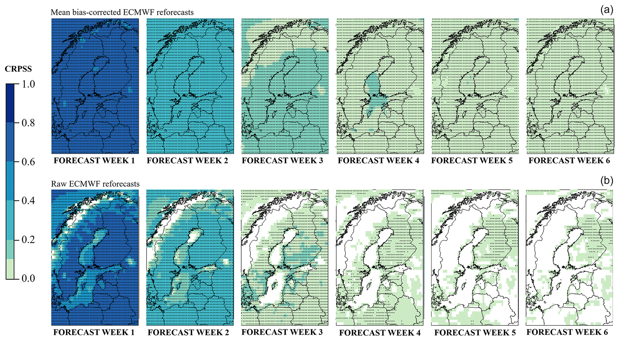
Figure 1Annual mean of the expected continuous ranked probability skill score (CRPSS) of the weekly mean temperature of the mean bias-corrected (a) and raw (b) ECMWF reforecasts for 1997–2016 using ERA-Interim climatology of 1981–2010 as the reference. The dotted areas represent the 95 % level of confidence that the CRPSS is above zero.
The European Centre for Medium-Range Weather Forecasts (ECMWF) has produced ERFs routinely since March 2002 (Vitart, 2014). The verification results of the ECMWF model's ERFs (Buizza and Leutbecher, 2015; Vitart, 2014) on a subcontinental and a regional scale (e.g. Monhart et al., 2018) demonstrated predictive skill beyond 2 weeks for temperature reforecasts over northern Europe. ECMWF uses the bias correction of the mean in their automatic products, removing the mean bias computed from the reforecasts, depending on the time of the year (Buizza and Leutbecher, 2015). We consider the bias over northern Europe not to be dependent only on the time of year but also on the prevailing weather pattern, and therefore, we aim to explore whether known teleconnections such as the strength of the stratospheric polar vortex and the phase of the Arctic Oscillation (AO) could be used to improve the forecasts.
The stratospheric polar vortex is an upper level low-pressure area that forms over both the northern and southern poles during winter due to the growing temperature gradient between the poles and the tropics. Strong westerly winds circulate the polar vortex, isolating the gradually cooling polar cap air. The strength of the northern polar vortex varies from year to year and can be indicated by, for example, the zonal mean zonal wind (ZMZW), at 60∘ N and 10 hPa, or polar cap temperatures. The stronger the circumpolar winds and the colder the polar cap temperatures are, the stronger the polar vortex will be. Planetary waves from the troposphere disturb the northern stratospheric polar vortex, leading to meandering and weakening of the westerlies and occasionally to the reverse, i.e. easterly flow (Schoeberl, 1978). This weakening of the stratospheric polar vortex also leads to warming of the polar cap temperatures, sometimes even > 30–40 K within several days. A warming of this magnitude, together with a reversal of the ZMZW at 60∘ N and 10 hPa, is commonly defined as a major sudden stratospheric warming (SSW), although other definitions have also been used (Butler et al., 2015).
During boreal winter, the strength of the polar vortex affects the phase of the AO, which characterises air mass flow between the Arctic and the midlatitudes. At the surface, the AO index is affected by the strength of the polar vortex, with a time lag of about 2–3 weeks (Baldwin and Dunkerton, 1999). A strong polar vortex is characterised by lower than average surface pressure in the Arctic, positive AO index, and strong westerly winds keeping the cold Arctic air locked in the polar region and bringing milder and wetter than average weather to northern Europe (Limpasuvan et al., 2005). In contrast, a weak polar vortex is characterised by higher than average surface pressure in the Arctic, negative AO index, and the meandering and/or weakening of the polar jet stream and tropospheric jet stream, enabling cold arctic/polar air outbreaks in northern Europe (Thompson et al., 2002; Tomassini et al., 2012).
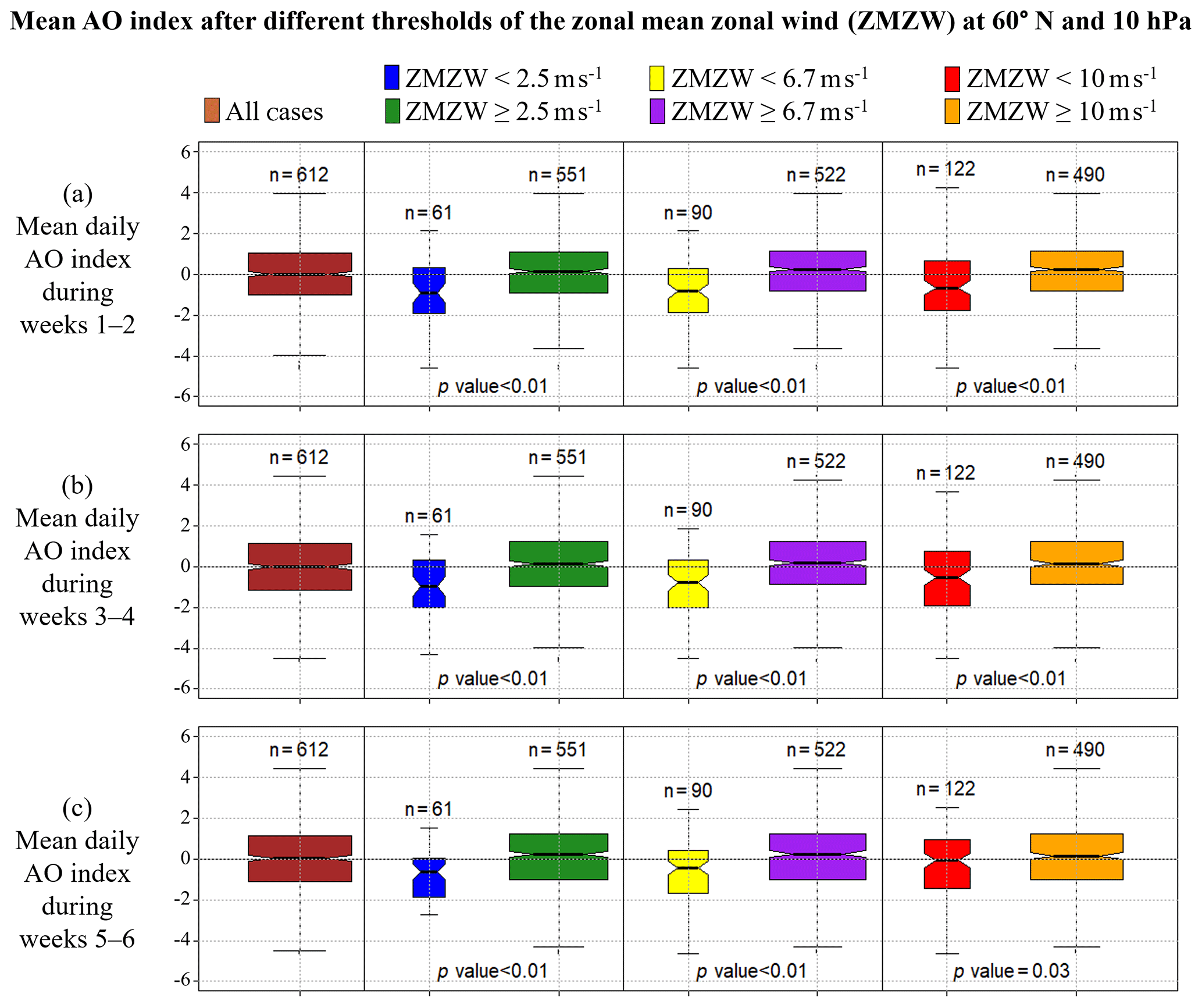
Figure 2Observed mean AO index in November–March (1981–2016; a) 1–2, (b) 3–4, and (c) 5–6 weeks after different thresholds of the zonal mean zonal wind (ZMZW) at 60∘ N and 10 hPa. The horizontal line dividing each box into two parts shows the median of the data, the ends of the box show the lower and upper quartiles, and the whiskers represent the highest and the lowest values, excluding outliers. The n written above each box indicates the number of observations in each group. The p value written below each boxplot pair indicates the likelihood of such a pair of distributions arising from a random sampling of a single distribution, as given by a Student's t test; i.e. p values less than 0.01 indicate that the means of the data sets differ significantly at the 99 % level of confidence. The notches of each side of the boxes were calculated by R boxplot.stats. If the notches of two plots do not overlap, then this is strong evidence that the two medians differ (Chambers et al., 1983).
During boreal winters, the strength of the stratospheric polar vortex influences the surface weather in the Northern Hemisphere within weeks or months (Baldwin and Dunkerton, 2001; Kidston et al., 2015), hence having the potential to forecast in that timescale. However, challenges related to the realistic modelling of the dynamical stratosphere–troposphere coupling have been adduced, for example, by Shepherd et al. (2018) and Polichtchouk et al. (2018). Therefore, we investigate if the known stratospheric–tropospheric connection could be used to improve the ERFs by statistical post-processing.
In this paper, we first verify the raw and the mean bias-corrected surface temperature reforecasts of the ECMWF's ERFs for forecast weeks 1 to 6 over northern Europe against the ERA-Interim surface temperature reanalysis (Dee et al., 2011). After that, our aim is to find out which thresholds of the ZMZW at 60∘ N and 10 hPa are followed by a statistically significantly weaker AO index. For this, we explore the observed daily AO index during boreal winters (1981–2016) 1–2, 3–4, and 5–6 weeks after different strengths of the observed the ZMZW at 60∘ N and 10 hPa. According to the observed daily AO index, after different thresholds of the ZMZW at 60∘ N and 10 hPa, we define a novel stratospheric wind indicator (SWI). For a statistically significantly weaker mean AO index, the SWI is defined as SWIneg; otherwise, SWI is defined as SWIplain. Furthermore, we study the mean surface temperature anomalies observed in northern Europe at 1–2, 3–4, and 5–6 weeks after SWIneg in comparison to SWIplain, and we utilise these anomalies in post-processing the temperature forecasts of the ECMWF reforecasts. Finally, we compare the SWI-based post-processed ECMWF reforecasts with the mean bias-corrected ECMWF reforecasts. Our paper is constructed as follows: first, we present the data sets and methods. Then, we present the results of the selection of the SWIneg and SWIplain and the skill scores of the forecasts with post-processing and without post-processing. In Sect. 4, we present our view on our findings and the possible next steps.
We verified and post-processed ERFs of the ECMWF's Integrated Forecasting System (IFS) cycle 43r1 (Vitart, 2014), which belongs to the models of the sub-seasonal to seasonal (S2S) prediction project of the World Weather Research Programme (WWRP) and World Climate Research Programme (WCRP; Vitart et al., 2017). These forecasts are run twice a week, on Mondays and Thursdays, in a horizontal resolution of 0.4∘. We first studied the weekly mean temperatures of the Monday runs over northern Europe (52 to 71.2∘ N and 10 to 33.2∘ E) with lead times of 1 to 6 weeks, here called forecast weeks 1 to 6. We verified the 20 years × 52 weeks =1040 reforecasts (11 members ensemble) for the 1997–2016 run for the same dates as the operational forecasts, i.e. Mondays in 2017. The weekly averages of the raw, mean bias-corrected (Sect. 2.2), and post-processed (Sect. 2.3 and 2.4) surface temperature forecasts over northern Europe were verified against the ERA-Interim 1981–2016 temperature reanalyses (Dee et al., 2011). Years 1981–2010 of the ERA-Interim data were used as the climatological reference period and as the statistical/climatological forecast.

Figure 3ERA-Interim observed (a–l) and ECMWF reforecasted (m–r) mean temperature anomalies in comparison to the 1981–2016 mean during boreal winters (November–February) in cases where the previous week's SWI was negative (SWIneg; covering about 17 % of the winter weeks) or plain (SWIplain; covering about 83 % of the winter weeks). The dotted areas represent the 95 % level of confidence where the means of surface temperature anomalies, after SWIneg and SWIplain, differ significantly.
2.1 Skill scores of the forecasts
A commonly used measure for probabilistic forecasts is the continuous ranked probability score (CRPS; Hersbach, 2000) as calculated with the following Eq. (1):
where F(y) and Fo(y) are the cumulative distribution functions of the forecast and the observation, respectively.
The CRPSs were calculated by the R package “scoringRules” (Jordan et al., 2019) for the ECMWF's reforecast (CRPSrf) and the climatological forecasts (ERA-Interim weekly mean temperatures in 1981–2010), which were used as the reference (CRPSclim). As the ensemble size of the reforecasts, m, was only 11, and the ensemble size of the operational forecasts of the ECMWF's IFS, M, was 51, the expected CRPS, namely the CRPSRF of the ECMWF's reforecast was calculated for 51 members using Eq. (26) in Ferro et al. (2008) as follows:
We calculated the annual means of the expected CRPSRF across all weeks (1 to 52) of the 1997–2016 reforecasts. These annual means were computed separately for lead times of 1 week, 2 weeks, 3 weeks, 4 weeks, 5 weeks, and 6 weeks, here called forecast week 1, forecast week 2, forecast week 3, forecast week 4, forecast week 5, and forecast week 6, respectively. Furthermore, the continuous ranked probability skill scores (namely the CRPSSs) of the annual mean CPRSs for each lead time were calculated as follows:
The statistical significances of each forecast week's annual mean CRPSS was determined for each grid point. The p value, with the null hypothesis that the CRPSS is zero, was calculated by a bootstrap resampling procedure with a replacement and a sample size of 5000 for significance level 0.05.
2.2 Bias correction of the ensemble mean
The mean bias correction (as in Buizza and Leutbecher, 2015, Eq. 7a) removed the mean bias computed from the ensemble reforecasts for the 20 years (1997–2016), depending on the forecast week date. For the 1997–2016 reforecasts, the average bias was calculated considering the ensemble reforecast members; i.e. 11 members' reforecasts with initial dates defined by 5 weeks centred on the forecast week date for the 19 years of reforecasts (1997–2016, excluding the reforecast year). The mean bias-corrected weekly mean temperatures were verified against the ERA-Interim data by calculating the annual mean CRPS separately for each lead time, i.e. forecast weeks 1 to 6. The skill scores of the mean bias-corrected forecasts and their statistical significance were calculated as explained in Sect. 2.1.
2.3 Definition of the stratospheric wind indicator (SWI)
As numerous observational and modelling studies have shown, the stratospheric polar vortex influences the weather in the Northern Hemisphere during boreal winter; strong polar vortex coincides more often with a positive AO index and mild surface weather in northern Europe, whereas weak polar vortex is more often followed by a negative AO index and cold air outbreaks (Thompson and Wallace, 1998, 2001; Kidston et al., 2015 and references therein). We aimed to find a stratospheric precursor for a statistically significantly weaker AO index available at the start of the forecast. The daily surface AO index was downloaded from the National Centers for Environmental Prediction (NCEP) and Climate Prediction Center (CPC). This daily AO index from the NCEP CPC is produced by projecting the daily 1000 hPa geopotential height anomalies north of 20∘ N onto the loading pattern of AO, which is defined as the first leading mode from the empirical orthogonal function (EOF) analysis of monthly mean 1000 hPa height anomalies poleward of 20∘ N during 1979–2000. As a precursor for the AO index, we used the daily ZMZW at 60∘ N and 10 hPa during 1981–2016 of the Modern-Era Retrospective analysis for Research and Applications, Version 2 (MERRA-2; Rienecker et al., 2011) reanalysis data provided by the National Aeronautics and Space Administration (NASA).
We explored the mean AO index 1 to 6 weeks after the beginning of each week in November–February (1981–2016) and the minimum daily ZMZW at 60∘ N and 10 hPa during the preceding 10 d to find a threshold for the ZMZW at 60∘ N and 10 hPa; this was to be followed by a statistically significantly weaker AO index 1–2, 3–4, and 5–6 weeks later. The statistical significance of the difference between the AO index, following the different thresholds of the ZMZW at 60∘ N and 10 hPa, was determined using a two-sided Student's t test with the null hypothesis that there is no difference. The threshold of the ZMZW at 60∘ N and 10 hPa for a statistically significantly weaker (at the 99 % confidence level) AO index observed 1–2, 3–4, and 5–6 weeks later, was used to define the SWI as follows: below the threshold the SWI was defined as negative (SWIneg) and above the threshold the SWI was defined as plain (SWIplain).

Figure 4Sensitivity of the expected CRPSSs of the post-processed ECMWF surface temperature reforecasts to the kSWI ranging from 0.0 to 1.0 in forecast weeks 3–4 (a, c) and 5–6 (b, d) in the cases of SWIneg (a, b) and SWIplain (c, d). The black boxes show the lower and upper quartiles, and the whiskers illustrate the extremes of the November–February mean CRPSSs for all the grid points in northern Europe.
2.4 Utilising the stratospheric winds indicator (SWI) in forecasting
In this section, we investigated the observed and reforecasted surface temperature anomalies 1–2, 3–4, and 5–6 weeks after SWIneg/SWIplain defined in Sect. 2.3. First, we calculated the 2-week mean temperature anomalies of the ERA-Interim reanalyses (Dee et al., 2011) of the 1–2, 3–4, and 5–6 weeks from the beginning of each week in January, February, November, and December in 1981–2016 in northern Europe. Subsequently, we divided the observed 2-week mean temperature anomalies into sets of anomalies, representing SWIneg and SWIplain, according to the minimum ZMZW at 60∘ N and 10 hPa during the preceding 10 d. Thereafter, we determined the statistical significance of the difference between the surface temperatures after SWIneg and SWIplain, using a two-sided Student's t test with the null hypothesis that there is no difference between SWIneg and SWIplain. This same procedure to define the difference between the surface temperatures after SWIneg and SWIplain was used for the ERA-Interim reanalyses for the period 1997–2016 to see how the selection of a shorter period affects the temperature anomalies. Furthermore, the mean surface temperature anomalies 1–2, 3–4, and 5–6 weeks after SWIneg and SWIplain in the ECMWF reforecasts run at the beginning of each week in November–February 1997–2016 were calculated to examine how the model reproduced the anomalies.
For post-processing the ECMWF reforecasts we calculated as TASWIneg and TASWIplain, representing mean temperature anomalies in November–February 1981–2016 after SWIneg and SWIplain, respectively. The TASWIneg and the TASWIplain were calculated separately for each grid point over northern Europe.
For the post-processing of the ECMWF reforecasts, we first defined the SWI as either SWIneg or SWIplain at the start of the forecast according to the minimum ZMZW at 60∘ N and 10 hPa during the preceding 10 d. According to the SWI, we added either TASWIneg or TASWIplain to the ERA-Interim mean temperature during 1981–2016, corresponding to forecast weeks 1–2, 3–4, and 5–6 to get SWIneg- and SWIplain-based mean temperatures, namely TSWIneg and TSWIplain, for weeks 1–2, 3–4, and 5–6, respectively. The TSWIneg and TSWIplain were used in post-processing the ECMWF reforecasts' mean bias-corrected ensemble members, TBC, by calculating a weighted average, TSWI_BC, for SWIneg as follows:
The same was done for SWIplain as follows:
where TSWI_BC was a post-processed ensemble member. kSWI was the weight of the TSWIneg or TSWIplain, which was tested between 0 and 1 and defined according to the best improvement in the skill scores of the post-processed forecast. With Eqs. (4) and (5), we adjusted each ensemble member with the same weight, and, hence, the original spread of the ECMWF reforecasts remained unchanged. The skill scores of the SWI-based post-processed forecasts, and their statistical significance, were calculated as explained in Sect. 2.1.

Figure 5Expected CRPSSs of forecast weeks 3–4 and 5–6 of the ECMWF's 2-week mean temperature reforecasts for November–February 1997–2016 in all cases (a–d), after SWIneg (e–h), and after SWIplain (i–l), with mean bias correction only (a, c, e, g, i, and k) and with both mean bias correction and SWI-based post-processing (b, d, f, h, j, and l). ERA-Interim climatology of 1981–2010 was used as the reference. The dotted areas represent the 95 % level of confidence that the CRPSS is above zero.
3.1 Skill scores of the forecasts
The annual mean of the expected CRPSS and its 95 % level of confidence of the raw and the mean bias-corrected (Sect. 2.2) weekly mean temperature of the ECMWF reforecasts for 1997–2016 are displayed in Fig. 1. In grid points where the CRPSS was higher than zero and the confidence level was higher than 95 % (dotted areas), the reforecasts were statistically significantly better than just the statistical forecast based on 1981–2010 climatology. Figure 1 illustrates that for forecast weeks 1–6 the mean bias-corrected ERF reforecasts were, on average, significantly better than the climatology. The annual mean CRPSS values show that in forecast weeks 1–3 the CRPSSs are, for the most part, above 0.1, whereas in forecast weeks 4–6 they are mostly lower, between 0 and 0.1.
3.2 The stratospheric observations and the AO index and surface temperature observed thereafter
Figure 2 shows boxplots of the observed mean of the daily AO index 1–2, 3–4, and 5–6 weeks after different strengths of the ZMZW at 60∘ N and 10 hPa. In Fig. 2 the first box (brown) represents the mean AO index after all the cases in November–February 1981–2016, i.e. 36 years ×17 weeks =612 cases. The blue, yellow, and red boxes in Fig. 2 show the mean AO index after cases in which the daily ZMZW at 60∘ N and 10 hPa was, during the preceding 10 d, below its 10th (2.5 ms−1), 15th (6.7 ms−1), and 20th (10 ms−1) percentile, respectively. The observed mean AO index was statistically significantly weaker at the 99 % confidence level 1–2, 3–4, and 5–6 weeks after the daily ZMZW at 60∘ N and 10 hPa had been below its overall wintertime 15th percentile, 6.7 ms−1. Based on this, we defined the SWI as negative (positive) and as indicating a statistically significantly lower (higher) AO index in cases where the minimum ZMZW at 60∘ N and 10 hPa was below (above) its 15th percentile, namely 6.7 ms−1, during the preceding 10 d.
Figure 3 shows the ERA-Interim (1981–2016 and 1997–2016) and model-forecasted mean temperature anomalies 1–6 weeks after SWIneg and SWIplain. Cases with ZMZW at 60∘ N and 10 hPa weaker than 6.7 ms−1, i.e. SWIneg, in Fig. 3a–c and g–i (stronger than 6.7 ms−1, i.e. SWIplain; Fig. 3d–f and j–l) were, on average, followed by colder (warmer) than average mean temperature. The ECMWF reforecasts (Fig. 3m–r) capture these mean anomalies clearly; in some areas they are even too strong in comparison to the ERA-Interim 1997–2016 (Fig. 3g–l).
3.3 The SWI and the forecasted mean temperatures
The mean temperature anomalies in Fig. 3a–f for northern Europe were used for the SWI-based post-processing as described in Sect. 2.4. Figure 4 shows how the post-processing based on the SWI affected the forecasting skill scores in the cases of SWIneg and SWIplain. The CRPSSs of the mean temperatures of the forecast weeks 3–4 and 5–6 were improved by the SWI-based post-processing, and the best median CRPSS was achieved by kSWI=0.3 for forecast weeks 3–4, in the cases of SWIplain, and by kSWI=0.6 for all the other cases.
Figure 5 shows the forecast skill of the mean bias-corrected mean temperature reforecasts of forecast weeks 3–4 and 5–6 in all cases (Fig. 5a and c), in cases where the ZMZW at 60∘ N and 10 hPa was below 6.7 ms−1 at the start of the forecast (SWIneg; Fig. 5e and g), and in cases where the ZMZW at 60∘ N and 10 hPa was above 6.7 ms−1 at the start of the forecast (SWIplain, Fig. 5i and k). In the cases of weak ZMZW at 60∘ N and 10 hPa at the start of the forecast (Fig. 5e and g) the CRPSSs of forecast weeks 3–4 and 5–6 reached even higher than 0.4 values in some areas, indicating their higher predictability in comparison with cases in which the ZMZW at 60∘ N and 10 hPa was stronger than 6.7 ms−1 at the start of the forecast (Fig. 5i and k).
Figure 5 also depicts the mean CRPSS of the mean bias-corrected and SWI post-processed reforecasts in all cases (Fig. 5b and d); in cases where the ZMZW at 60∘ N and 10 hPa was below 6.7 ms−1 (SWIneg) at the start of the forecast (kSWI=0.6 and kSWI=0.6 in Fig. 5e and g, respectively), and in cases where the ZMZW at 60∘ N and 10 hPa was above 6.7 ms−1 (SWIplain) at the start of the forecast (kSWI=0.3 and kSWI=0.6 in Fig. 5j and l, respectively). In comparison to the only mean bias-corrected ECMWF reforecasts (see Fig. 5a, c, e, g, i, and k), by adding the SWI-based post-processing to the ECMWF reforecasts (see Fig. 5b, d, f, h, and j) the CRPSSs for weeks 3–4 and 5–6 were slightly improved, and the area of these forecasts was expanded for being significantly better than just the climatological forecast.
Based on ECMWF's extended-range reforecasts for the period 1997–2016, we found that the weekly mean surface temperature forecasts over northern Europe were, on average, significantly better than just the climatological forecast in weeks 1–6, however, in weeks 4–6, the CRPSSs were quite low and mostly between 0 and 0.1.
We studied the mean AO index after different thresholds of ZMZW at 60∘ N and 10 hPa. We found that the mean AO index was statistically significantly weaker 1–2, 3–4, and 5–6 weeks after the daily ZMZW at 60∘ N and 10 hPa had been below its November–February 15th percentile at 6.7 ms−1.
Cases preceded by weaker (stronger) than 6.7 ms−1 ZMZW at 60∘ N and 10 hPa were defined as SWIneg (SWIplain). As a negative AO index enables cold air outbreaks in northern Europe (Thompson et al., 2002; Tomassini et al., 2012) and a positive AO index tends to bring milder and wetter than average weather to northern Europe (Limpasuvan et al., 2005), we investigated how the mean surface temperatures were in November–February (1981–2016) in northern Europe 1–6 weeks after SWIneg/SWIplain. We found that the mean surface temperature anomalies in northern Europe in November–February in 1981–2016 after SWIneg and SWIplain were, in many places, statistically significantly different, with anomalously cold surface temperatures more common 1–6 weeks after SWIneg. The mean temperature anomalies corresponding to SWIneg/SWIplain were used in post-processing the ECMWF's mean temperature reforecast for weeks 3–4 and 5–6 in northern Europe during boreal winter, and, thereby, those weeks' forecast skills were slightly improved.
We also investigated the forecast skill in the cases of ZMZW at 60∘ N and 10 hPa below or above the threshold of 6.7 ms−1. We found that the cases of weaker than 6.7 ms−1 ZMZW at 60∘ N and 10 hPa at the start of the forecast were followed by higher than average forecasting skill scores of mean surface temperature for forecast weeks 3–4 and 5–6. Also, earlier studies have reported enhanced forecast skill during periods of negative AO; for example, in 500 hPa geopotential height forecasts in the northern midlatitudes in both the medium range (Langland and Maue, 2012) and extended range (Minami and Takaya, 2020).
In future the SWI-based post-processing method introduced in this paper could also be tested for other northern areas affected by the polar vortex and for precipitation and windiness forecasts, and it could be further developed by, for example, the Madden–Julian oscillation (Madden and Julian, 1994; Zhang, 2005; Jiang et al., 2017; Vitart, 2017; Vitart and Molteni, 2010; Robertson et al., 2018, Cassou, 2008) and the quasi-biennial oscillation (Watson and Gray, 2014; Scaife et al., 2014; Garfinkel et al., 2018; Gray et al., 2018). In this study, the effect of global warming was not filtered from the temperature anomalies used for statistical post-processing. In future work, the impact of filtering the effect of global warming could be tested. Moreover, the next step would be looking for the stratospheric signal from the forecast model.
The ERA-Interim reanalysis data were retrieved from the ECMWF's Meteorological Archival and Retrieval System (MARS) at https://apps.ecmwf.int/datasets/data/interim-full-daily/levtype=sfc/ (MARS, 2020a). The ERF data of the ECMWF’s IFS cycle 43r1 were retrieved from the ECMWF's MARS archive at https://apps.ecmwf.int/mars-catalogue/ (MARS, 2020b). The daily AO index was downloaded from the CPC of the NCEP, National Oceanic and Atmospheric Administration at https://www.cpc.ncep.noaa.gov/products/precip/CWlink/daily_ao_index/ao.shtml (CPC, 2020). The daily ZMZW at 60∘ N and 10 hPa data of the MERRA-2 reanalysis by NASA’s Atmospheric Chemistry and Dynamics Laboratory was downloaded from https://acd-ext.gsfc.nasa.gov/Data_services/met/ann_data.html (ACDL, 2020). The data of Figs. 1–5 are available at https://etsin.fairdata.fi/dataset/34d0f8b3-a593-46aa-8fcf-358d72f6cac1 (Korhonen, 2020).
NK designed the study, analysed the results, and prepared the paper with contributions from all co-authors. OH participated in the study design and analysed the results. MK contributed to the discussions and fine-tuned the experiments. DSR contributed to the discussions and to the interpretation of the results. HJ provided supervision during the experiments and writing. HG contributed to the study design and was in charge of the management and the acquisition of the financial support for the CLIPS project that led to this publication.
The authors declare that they have no conflict of interest.
We acknowledge the ECMWF for the monthly forecast data and ERA-Interim data, NOAA/CPC for providing the AO index data, and NASA for providing the 10 hPa wind data. We thank the CLIPS team and the developers of the CRAN R calculation package for “scoringRules”. We thank the three anonymous reviewers for their good and constructive comments.
This research has been supported by the Academy of Finland (grant no. 303951; SA CLIPS).
This paper was edited by Peter Haynes and reviewed by three anonymous referees.
ACDL: Atmospheric Chemistry and Dynamics Laboratory of the National Aeronautics and Space Administration, Annual Meteorological Statistics, available at: https://acd-ext.gsfc.nasa.gov/Data_services/met/ann_data.html, last access: 11 July 2020.
Baldwin, M. P. and Dunkerton, T. J.: Propagation of the Arctic Oscillation from the stratosphere to the troposphere, J. Geophys. Res, 104, 30937–30946, https://doi.org/10.1029/1999JD900445, 1999.
Baldwin, M. P. and Dunkerton, T. J.: Stratospheric harbingers of anomalous weather regimes, Science, 294, 581–584, https://doi.org/10.1126/science.1063315, 2001.
Buizza, R. and Leutbecher, M.: The forecast skill horizon, Q. J. Roy. Meteor. Soc., 141, 3366–3382, https://doi.org/10.1002/qj.2619, 2015.
Butler, A. H., Seidel, D. J., Hardiman, S. C., Butchart, N., Birner, T., and Match, A.: Defining sudden stratospheric warmings, B. Am. Meteorol. Soc., 96, 1913–1928, https://doi.org/10.1175/BAMS-D-13-00173.1, 2015.
Cassou, C.: Intraseasonal interaction between the Madden–Julian Oscillation and the North Atlantic Oscillation, Nature, 455, 523–527, 2008.
Chambers, J. M., Cleveland, W. S., Kleiner, B, and Tukey, P.A.: Graphical Methods for Data Analysis, The Wadsworth statistics/probability series, Wadsworth and Brooks/Cole, Pacific Grove, CA, 1983.
CPC: Climate Prediction Center of the National Centers for Environmental Prediction, National Oceanic and Atmospheric Administration, Climate and Weather linkage, available at: https://www.cpc.ncep.noaa.gov/products/precip/CWlink/daily_ao_index/ao.shtml, last access: 11 July 2020.
Dee, D. P., Uppala, S. M., Simmons, A. J., Berrisford, P., Poli, P., Kobayashi, S., Andrae, U., Balmaseda, M. A., Balsamo, G., Bauer, P., Bechtold, P., Beljaars, A. C. M., van de Berg, L., Bidlot, J., Bormann, N., Delsol, C., Dragani, R., Fuentes, M., Geer, A. J., Haimberger, L., Healy, S. B., Hersbach, H., Hólm, E. V., Isaksen, L., Kållberg, P., Köhler, M., Matricardi, M., McNally, A. P., Monge-Sanz, B. M., Morcrette, J.-J., Park, B.-K., Peubey, C., de Rosnay, P., Tavolato, C., Thépaut, J.-N., and Vitart, F.: The ERA-Interim reanalysis: configuration and performance of the data assimilation system, Q. J. Roy. Meteor. Soc., 137, 553–597, 2011.
Ervasti, T., Gregow, H., Vajda, A., Laurila, T. K., and Mäkelä, A.: Mapping users' expectations regarding extended-range forecasts, Adv. Sci. Res., 15, 99–106, https://doi.org/10.5194/asr-15-99-2018, 2018.
Ferro, C. A. T., Richardson, D. S., and Weigel, A. P.: On the effect of ensemble size on the discrete and continuous ranked probability scores, Meteorol. Appl., 15, 19–24, https://doi.org/10.1002/met.45, 2008.
Garfinkel, C. I., Schwartz, C., Domeisen, D. I. P., Son, S-W., Butler, A. H., and White, I. P.: Extratropical stratospheric predictability from the Quasi-Biennial Oscillation in Subseasonal forecast models, J. Geophys. Res.-Atmos., 123, 7855–7866, https://doi.org/10.1029/2018JD028724, 2018.
Gray, L. J., Anstey, J. A., Kawatani, Y., Lu, H., Osprey, S., and Schenzinger, V.: Surface impacts of the Quasi Biennial Oscillation, Atmos. Chem. Phys., 18, 8227–8247, https://doi.org/10.5194/acp-18-8227-2018, 2018.
Hersbach, H.: Decomposition of the continuous ranked probability score for ensemble prediction systems, Weather Forecast., 15, 559–570, https://doi.org/10.1175/1520-0434(2000)015<0559:DOTCRP>2.0.CO;2, 2000.
Jiang, Z., Feldstein, S. B., and Lee S.: The relationship between the Madden–Julian Oscillation and the North Atlantic Oscillation, Q. J. Roy. Meteor. Soc., 143, 240–250, https://doi.org/10.1002/qj.2917, 2017.
Jordan, A., Krueger, F., and Lerch, S.: Evaluating Probabilistic Forecasts with scoringRules, J. Stat. Softw., 90, 1–37, https://doi.org/10.18637/jss.v090.i12, 2019.
Kidston, J., Scaife, A. A., Hardiman, S. C., Mitchell, D. M., Butchart, N., Baldwin, M. P., and Gray, L. J.: Stratospheric influence on tropospheric jet streams, storm tracks and surface weather, Nat. Geosci., 8, 433–440, 2015.
Korhonen, N.: Files containing data in Figures 1–5 in the manuscript Korhonen N. et al. “Adding value to Extended-range Forecasts in Northern Europe by Statistical Post-processing Using Stratospheric Observations”, available at: https://etsin.fairdata.fi/dataset/34d0f8b3-a593-46aa-8fcf-358d72f6cac1, last access: 11 July 2020.
Langland, R. H. and Maue, R. N.: Recent Northern Hemisphere mid-latitude medium-range deterministic forecast skill, Tellus A, 64, 17531, https://doi.org/10.3402/tellusa.v64i0.17531, 2012.
Limpasuvan, V., Hartmann, D. L., Thompson, D. W. J., Jeev, K., and Yung, Y. L.: Stratosphere-troposphere evolution during polar vortex intensification, J. Geophys. Res., 110, D24101, https://doi.org/10.1029/2005JD006302, 2005.
Madden, R. A. and Julian, P. R.: Observations of the 40–50-day tropical oscillation–A review, Mon. Weather Rev., 122, 814–837, 1994.
MARS: ERA-Interim reanalysis data, available at: https://apps.ecmwf.int/datasets/data/interim-full-daily/levtype=sfc/ (last access: 11 July 2020a).
MARS: ERF data of the European Centre for Medium-Range Weather Forecasts’ Integrated Forecasting System cycle 43r1, available at: https://apps.ecmwf.int/mars-catalogue/, last access: 11 July 2020b.
Minami, A. and Takaya, Y.: Enhanced Northern Hemisphere Correlation Skill of Subseasonal Predictions in the Strong Negative Phase of the Arctic Oscillation, J. Geophys. Res.-Atmos., 125, e2019JD031268, https://doi.org/10.1029/2019JD031268, 2020.
Monhart, S., Spirig, C., Bhend, J., Bogner, K., Schär, C., and Liniger, M. A.: Skill of subseasonal forecasts in Europe: Effect of bias correction and downscaling using surface observations, J. Geophys. Res.-Atmos., 123, 7999–8016, 2018.
Polichtchouk, I., Shepherd, T. G., and Byrne, N. J.: Impact of Parametrized Nonorographic Gravity Wave Drag on Stratosphere-Troposphere Coupling in the Northern and Southern Hemispheres, Geophys. Res. Lett., 45, 8612–8618, https://doi.org/10.1029/2018gl078981, 2018.
Rienecker, M. M., Suarez, M. J., Gelaro, R., Todling, R., Emily Liu, J. B., Bosilovich, M. G., Schubert, S. D., Takacs, L., Kim, G. K., Bloom, S., Chen, J., Collins, D., Conaty, A., da Silva, A., Gu, W., Joiner, J., Koster, R. D., Lucchesi, R., Molod, A., Owens, T., Pawson, S., Pegion, P., Redder, C. R., Reichle, R., Robertson, F. R., Ruddick, A. G., Sienkiewicz, M., and Woollen, J.: MERRA: NASA's modern-era retrospective analysis for research and applications, J. Climate, 24, 3624–3648, https://doi.org/10.1175/JCLI-D-11-00015.1, 2011.
Robertson, A. W., Camargo, S. J., Sobel, A., Vitart, F., and Wang, S.: Summary of workshop on sub-seasonal to seasonal predictability of extreme weather and climate, npj Climate and Atmospheric Science, 1, 20178, https://doi.org/10.1038/s41612-017-0009-1, 2018.
Scaife, A. A., Athanassiadou, M., Andrews, M., Arribas, A., Baldwin, M., Dunstone, N., Knight, J., MacLachlan, C., Manzini, E., Müller, W. A., Holger Pohlmann, H., Smith, D., Stockdale, T., and Williams, A.: Predictability of the quasi-biennial oscillation and its northern winter teleconnection on seasonal to decadal timescales, Geophys. Res. Lett., 41, 1752–1758, https://doi.org/10.1002/2013GL059160, 2014.
Schoeberl, M. R.: Stratospheric warmings: Observations and theory, Rev. Geophys., 16, 521–538, 1978.
Shepherd T. G., Polichtchouk, I., Hogan, R., and Simmons, A. J.: Report on Stratosphere Task Force, ECMWF Technical Memorandum, no. 824, https://doi.org/10.21957/0vkp0t1xx, 2018.
Thompson, D. W. J. and Wallace, J. M.: The Arctic Oscillation signature in the wintertime geopotential height and temperature fields, Geophys. Res. Lett., 25, 1297–1301, 1998.
Thompson, D. W. J. and Wallace, J. M.: Regional Climate Impacts of the Northern Hemisphere Annular Mode, Science, 293, 85–89, 2001.
Thompson, D. W. J., Baldwin, M. P., and Wallace J. M.: Stratospheric connection to Northern Hemisphere wintertime weather: implications for prediction, J. Climate, 15, 1421–1428, 2002.
Tomassini, L., Gerber, E. P., Baldwin, M. P., Bunzel, F., and Giorgetta, M.: The role of stratosphere troposphere coupling in the occurrence of extreme winter cold spells over northern Europe, J. Adv. Model. Earth Sy., 4, M00A03, https://doi.org/10.1029/2012MS000177, 2012.
Vitart, F.: Evolution of ECMWF sub-seasonal forecast skill scores, Q. J. Roy. Meteor. Soc., 140, 1889–1899, https://doi.org/10.1002/qj.2256, 2014.
Vitart, F.: Madden-Julian Oscillation prediction and teleconnections in the S2S database: MJO prediction and teleconnections in the S2S database, Q. J. Roy. Meteor. Soc., 143, 2210–2220, 2017.
Vitart, F. and Molteni, F.: Simulation of the MJO and its teleconnections in the ECMWF forecast system, Q. J. Roy. Meteor. Soc., 136, 842–855, 2010.
Vitart, F., Ardilouze, C., Bonet, A., Brookshaw, A., Chen, M., Codorean, C., Déqué, M., Ferranti, L., Fucile, E., Fuentes, M., Hendon, H., Hodgson, J., Kang, H., Kumar, A., Lin, H., Liu, G., Liu, X., Malguzzi, P., Mallas, I., Manoussakis, M., Mastrangelo, D., MacLachlan, C., McLean, P., Minami, A., Mladek, R., Nakazawa, T., Najm, S., Nie, Y., Rixen, M., Robertson, A. W., Ruti, P., Sun, C., Takaya, Y., Tolstykh, M., Venuti, F., Waliser, D., Woolnough, S., Wu, T., Won, D., Xiao, H., Zaripov, R., and Zhang L.: The Subseasonal to Seasonal (S2S) Prediction Project Database, B. Am. Meteorol. Soc., 98, 163–173, https://doi.org/10.1175/BAMS-D-16-0017.1, 2017.
Watson, P. A. and L. J. Gray: How Does the Quasi-Biennial Oscillation Affect the Stratospheric Polar Vortex?, J. Atmos. Sci., 71, 391–409, https://doi.org/10.1175/JAS-D-13-096.1, 2014.
Zhang, C.: Madden-Julian Oscillation, Rev. Geophys., 43, RG2003, https://doi.org/10.1029/2004RG000158, 2005.