Inverse modeling of SO₂ and NO_x emissions over China using multisensor satellite data – Part 2: Downscaling techniques for air quality analysis and forecasts

Top-down emission estimates provide valuable up-to-date information on pollution sources; however, the computational effort and spatial resolution of satellite products involved with developing these emissions often require them to be estimated at resolutions that are much coarser than is necessary for regional air quality forecasting. This work thus introduces several approaches to downscaling coarse-resolution ($\mathrm{2}{}^{\circ }\times \mathrm{2.5}{}^{\circ }$) posterior SO₂ and NO_x emissions for improving air quality assessment and forecasts over China in October 2013. As in Part 1 of this study, these $\mathrm{2}{}^{\circ }\times \mathrm{2.5}{}^{\circ }$ posterior SO₂ and NO_x emission inventories are obtained from GEOS-Chem adjoint modeling with the constraints of OMPS SO₂ and NO₂ products retrieved at 50 km×50 km at nadir and $\sim \mathrm{190}\mathrm{km}\times \mathrm{50}\mathrm{km}$ at the edge of ground track. The prior emission inventory (MIX) and the posterior GEOS-Chem simulations of surface SO₂ and NO₂ concentrations at coarse resolution underestimate observed hot spots, which is called the coarse-grid smearing (CGS) effect. To mitigate the CGS effect, four methods are developed: (a) downscale $\mathrm{2}{}^{\circ }\times \mathrm{2.5}{}^{\circ }$ GEOS-Chem surface SO₂ and NO₂ concentrations to the resolution of $\mathrm{0.25}{}^{\circ }\times \mathrm{0.3125}{}^{\circ }$ through a dynamic downscaling concentration (MIX-DDC) approach, which assumes that the $\mathrm{0.25}{}^{\circ }\times \mathrm{0.3125}{}^{\circ }$ simulation using the prior MIX emissions has the correct spatial distribution of SO₂ and NO₂ concentrations but a systematic bias; (b) downscale surface NO₂ simulations at $\mathrm{2}{}^{\circ }\times \mathrm{2.5}{}^{\circ }$ to $\mathrm{0.05}{}^{\circ }\times \mathrm{0.05}{}^{\circ }$ according to the spatial distribution of Visible Infrared Imaging Radiometer Suite (VIIRS) nighttime light (NL) observations (e.g., NL-DC approach) based on correlation between VIIRS NL intensity with TROPOspheric Monitoring Instrument (TROPOMI) NO₂ observations; (c) downscale posterior emissions (DE) of SO₂ and NO_x to $\mathrm{0.25}{}^{\circ }\times \mathrm{0.3125}{}^{\circ }$ with the assumption that the prior fine-resolution MIX inventory has the correct spatial distribution (e.g., MIX-DE approach); and (d) downscale posterior NO_x emissions using VIIRS NL observations (e.g., NL-DE approach). Numerical experiments reveal that (a) using the MIX-DDC approach, posterior SO₂ and NO₂ simulations improve on the corresponding MIX prior simulations with normalized centered root mean square error (NCRMSE) decreases of 63.7 % and 30.2 %, respectively; (b) the posterior NO₂ simulation has an NCRMSE that is 17.9 % smaller than the prior when they are both downscaled through NL-DC, and NL-DC is able to better mitigate the CGS effect than MIX-DDC; (c) the simulation at $\mathrm{0.25}{}^{\circ }\times \mathrm{0.3125}{}^{\circ }$ using the MIX-DE approach has NCRMSEs that are 58.8 % and 14.7 % smaller than the prior $\mathrm{0.25}{}^{\circ }\times \mathrm{0.3125}{}^{\circ }$ MIX simulation for surface SO₂ and NO₂ concentrations, respectively, but the RMSE from the MIX-DE posterior simulation is slightly larger than that from the MIX-DDC posterior simulation for both SO₂ and NO₂; (d) the NL-DE posterior NO₂ simulation also improves on the prior MIX simulation at $\mathrm{0.25}{}^{\circ }\times \mathrm{0.3125}{}^{\circ }$, but it is worse than the MIX-DE posterior simulation; (e) in terms of evaluating the downscaled SO₂ and NO₂ simulations simultaneously, using the posterior SO₂ and NO_x emissions from joint inverse modeling of both species is better than only using one (SO₂ or NO_x) emission from corresponding single-species inverse modeling and is similar to using the posterior emissions of SO₂ and NO_x emission inventories respectively from single-species inverse modeling.

Forecasts of surface concentrations for November 2013 using the posterior emissions obtained by applying the posterior MIX-DE emissions for October 2013 with the monthly variation information derived from the prior MIX emission inventory show that (a) the improvements of forecasting surface SO₂ concentrations through MIX-DE and MIX-DDC are comparable; (b) for the NO₂ forecast, MIX-DE shows larger improvement than NL-DE and MIX-DDC; (c) NL-DC is able to better decrease the CGS effect than MIX-DE but shows larger NCRMSE; (d) the forecast of surface O₃ concentrations is improved by MIX-DE downscaled posterior NO_x emissions. Overall, for practical forecasting of air quality, it is recommended to use satellite-based observation already available from the last month to jointly constrain SO₂ and NO₂ emissions at coarser resolution and then downscale these posterior emissions at finer spatial resolution suitable for regional air quality modeling for the present month.

1 Introduction

Simulations and forecasts of surface concentrations of SO₂ and NO₂, the two criteria pollutants in the atmosphere defined by the US EPA and China, are important for studying their impacts on air quality and public health (Ghozikali et al., 2016). Their accuracy depends not only on reliability of meteorological fields and correct representation of chemical processes in the air quality model (Gao et al., 2016; Ge et al., 2017) but also on the fidelity of the emissions used in the latter. For the same region and time, different emission inventories can lead to differences of up to 100 % for surface SO₂ and NO₂ simulations (Y. Wang et al., 2016). Additionally, model resolution also plays an important role (Kharol et al., 2017), as the simulated concentration of these short-lived species only represents the average of a grid cell in which the high concentrations of SO₂ and NO₂ from source regions and (or) strong spatial variation of these species are smeared out. This is called the coarse-grid smearing (CGS) effect, and it depends on the species lifetimes, the spatial distribution of emissions, and the model (and inventory) resolution. The lifetime for SO₂ in the lower troposphere is less than 1 d in the summer and 1 or 2 d in winter (Lee et al., 2011), and it is several hours for NO₂ (Lin et al., 2010); their smearing length scales (Palmer et al., 2003) are on the order of 100 km (Lee et al., 2011; Martin et al., 2003). Xing et al. (2015) showed that surface SO₂ and NO₂ concentrations from the Weather Research and Forecasting Model (WRF)–Community Multiscale Air Quality (CMAQ) model simulations at 108 km×108 km resolution were underestimated when evaluated with urban network observations and overestimated relative to rural networks.

Obtaining accurate and timely emission estimates can be challenging. The bottom-up approach, which integrates activity data and emission factors, is widely used to generate inventories (Li et al., 2017a; Janssens-Maenhout et al., 2015; Kurokawa et al., 2013). These bottom-up emissions have uncertainties larger than 30 % at the regional scale for both SO₂ and NO_x over China (Kurokawa et al., 2013; Li et al., 2017a). When used to simulate air quality with a chemical transport model (CTM), these emission estimates are gridded to regular grid cells (of ∼ 1^∘ or finer) through locations of major manufacturing facilities and power plants and proxy data such as population distributions and road networks (Zheng et al., 2017; Streets et al., 2003). Consequently, uncertainties of emission estimates at the grid-cell scale are larger than at the country scale. Moreover, bottom-up inventories usually have a time lag of at least 1 year, as it takes time to collect all the data required to generate them (Liu et al., 2018). Outdated emission inventories increase the uncertainty of simulations and forecasts, especially for China where emissions change quickly due to rapid economic development and implementation of emission control policies (Zheng et al., 2018; Y. Wang et al., 2016).

Over the past two decades, many satellites have provided vertical column density (VCD) data of SO₂ and NO₂ and aerosol optical depth (AOD) retrievals globally; these data have been used to constrain emission estimates with the following approaches at various spatial resolutions. The mass balance approach (Lee et al., 2011; Martin et al., 2003; Koukouli et al., 2018) and the finite-difference mass balance method (Lamsal et al., 2011) were developed to use VCD retrievals of SO₂ and NO₂ from the Global Ozone Monitoring Experiment (GOME), GOME-2, SCanning Imaging Absorption spectroMeter for Atmospheric CHartographY (SCIAMACHY), Ozone Monitoring Instrument (OMI), and Ozone Mapper and Profiler Suite (OMPS) to constrain SO₂ and NO_x emissions at spatial resolutions in the range of 25 to 250 km. The accuracy, however, decreases as spatial resolution becomes finer (Turner et al., 2012), because the transport is not explicitly accounted for in these approaches. The emission strength of SO₂ point sources that are larger than 30 kt yr⁻¹ can be estimated through a linear regression between OMI VCDs and emission strength (Fioletov et al., 2016), and the approach was used to build a global SO₂ emission inventory at $\mathrm{0.1}{}^{\circ }\times \mathrm{0.1}{}^{\circ }$ (Liu et al., 2018). Advanced data assimilation approaches including the four-dimension variational data assimilation (4D-Var) (Qu et al., 2019a, b, 2017; Y. Wang et al., 2016a, 2020; Wang et al., 2012; Xu et al., 2013; Kurokawa et al., 2009) and the ensemble Kalman filter (EnKF) approach (Miyazaki et al., 2012, 2017) were developed to use satellite SO₂ and NO₂ columns densities and AOD retrievals to constrain emissions at low spatial resolutions (> 50 km) as these approaches are computationally intensive. Some variations of the 4D-Var and Kalman filter approaches were developed to save computational time at the expense of accuracy or temporal resolution (Qu et al., 2017; Kong et al., 2019; Mijling and van der A, 2012; Ding et al., 2015).

The mismatch among the resolutions of emission inventories, CTMs, and satellite observations has prompted previous development of downscaling methods. For example, the popular OMI has a footprint size of 13 km×24 km at nadir and 26 km×128 km at the swath edge that is too coarse to capture the urban NO₂ plume without oversampling. Consequently, a spatial weighting kernel derived from the CMAQ simulation at finer spatial resolution was developed to downscale OMI NO₂ retrievals to 1.33 km×1.33 km (Kim et al., 2018, 2016; Goldberg et al., 2017). The resulting high-spatial-resolution OMI NO₂ data was further applied to constrain emissions, which showed an underestimate in the bottom-up NO_x inventories in Seoul, South Korea, during the Korea–United States Air Quality Study (KORUS-AQ) (Goldberg et al., 2019). In cases where model grid cells are larger than satellite footprints, Lamsal et al. (2008) applied the ratio between the local OMI NO₂ column to mean OMI field over a $\mathrm{2}{}^{\circ }\times \mathrm{2.5}{}^{\circ }$ GEOS-Chem grid cell to derive local surface-VCD scaling factors, which were used to infer improved surface NO₂ concentrations. An inverse distance weighting technique was applied to interpolate emissions and initial and boundary species conditions from coarse resolution to fine resolution for nested CTM simulations (Yahya et al., 2017, 2016; Hong et al., 2017), but it was not able to capture hot spots in the downscaled fields.

The CGS effect, combined with the sharp spatial variations of surface SO₂ and NO₂ concentrations, introduces challenges when comparing model simulations with in situ observations. Y. Wang et al. (2016) showed the improvement when using posterior SO₂ emissions constrained by OMI SO₂ to simulate surface SO₂ concentrations at a resolution of $\mathrm{2}{}^{\circ }\times \mathrm{2.5}{}^{\circ }$ . However, this was illustrated for a rural site that is ∼ 100 km away from Beijing's urban center, and there are no strong SO₂ sources around it, which means the CGS effect is minimal at this site. Kharol et al. (2015, 2017) found that surface SO₂ and NO₂ concentrations derived through scaling OMI SO₂ and NO₂ VCDs with vertical profiles from a CTM at a resolution of $\mathrm{0.1}{}^{\circ }\times \mathrm{0.1}{}^{\circ }$ are a factor of 2 smaller than US EPA in situ observations. These underestimations are partly ascribed to the CGS effect, although uncertainty in vertical profiles also plays a role (Kharol et al., 2015, 2017; Bechle et al., 2013). They further showed that the underestimation decreases significantly when in situ observations are converted to represent the averages of larger areas through a linear regression function which is built by comparing simulations of SO₂ between two spatial resolutions of 2.5 km×2.5 km and 30 km×30 km.

This paper, as the second of a two-part study, aims at using SO₂ and NO_x emissions constrained by OMPS SO₂ and NO₂ retrievals through 4D-Var (which is presented in Part 1, i.e., Wang et al., 2020) to improve air quality forecasts. Since the emission inventories in Part 1 are derived at the $\mathrm{2}{}^{\circ }\times \mathrm{2.5}{}^{\circ }$ resolution to save computational resources and to account for the coarse spatial resolution of satellite data used (e.g., OMPS SO₂ and NO₂), the focus here is to develop novel methods to downscale coarse-resolution emission inventories or simulation results to generate fine-resolution surface SO₂ and NO₂ concentrations and evaluate them from an air quality forecasting point of view. High-resolution bottom-up emission inventories and Visible Infrared Imaging Radiometer Suite (VIIRS) nighttime lights contain geospatial information (such as roads, location of power plants, and residential areas) in fine spatial resolution for downscaling coarser-resolution anthropogenic emissions. Indeed, VIIRS nighttime light observations are shown to be good indicators of socioeconomic parameters including urbanization, economic activity, population (Bennett and Smith, 2017), and road density (Levin and Zhang, 2017) and have been used to map CO₂ emissions (Ou et al., 2015) and derive surface PM_2.5 concentrations at nighttime (J. Wang et al., 2016). Thus, it should also be promising to build relationships between VIIRS nighttime lights and both NO₂ in the atmosphere and NO_x emissions, which will be assessed here for their application in downscaling surface NO₂ concentrations and NO_x emissions.

We introduce data in Sect. 2. Section 3 presents the models for simulations and forecasts of surface SO₂ and NO₂, as well as the downscaling approaches. The improvements in the simulations and forecasts through various downscaling methods are provided in Sect. 4. Discussions of implications of the results and conclusions are followed in Sect. 5.

2 Data

2.1 In situ data of surface SO₂, NO₂, and O₃

We obtained the in situ measurements of surface SO₂, NO₂, and O₃ from the China National Environmental Monitoring Center for model evaluation. SO₂ and NO₂ are measured by various commercial instruments using the ultraviolet fluorescence method and the chemiluminescence method, respectively (Zhang and Cao, 2015). In the chemiluminescence method NO₂ observations are obtained by measuring NO from decomposed NO₂. This can result in a positive bias because NO_z (all compounds that are products of the atmospheric oxidation of NO_x) will also be reduced to NO. Steinbacher et al. (2007) showed that the ratio of NO₂ to NO_z ($r_{{\mathrm{NO}}_{\mathrm{2}}}$) depends on the distance that NO₂ plumes transport from the source. In other words, the longer the distance, the more the potential for oxidation of NO₂ and hence the smaller $r_{{\mathrm{NO}}_{\mathrm{2}}}$; only 43 %–76 % and 70 %–83 % of real NO₂ contribute to the measured value (NO₂)_m for rural and urban sites, respectively (Steinbacher et al., 2007). For this study, as observational sites are in cities, a maximum value of 0.83 is used to convert (NO₂)_m measurements to the NO₂ concentrations, which are subsequently used for evaluating the model results. Additionally, we also test values for $r_{{\mathrm{NO}}_{\mathrm{2}}}$ in the range of 0.7 to 1.0.

2.2 VIIRS data for artificial light

The VIIRS on board the Suomi National Polar-orbiting Partnership (Suomi NPP) satellite was launched on 28 October 2011, and its day/night band (DNB) provides observations of nighttime lights with a spatial resolution of 750 m (Miller et al., 2013). Here, we use the VIIRS nighttime lights product that has excluded background noise as well as solar and lunar contamination and has screened out the data degraded by cloud cover and features unrelated to electric lighting (Elvidge et al., 2017a). This product is regridded to $\mathrm{0.05}{}^{\circ }\times \mathrm{0.05}{}^{\circ }$ for October 2013 and to $\mathrm{0.05}{}^{\circ }\times \mathrm{0.05}{}^{\circ }$ and $\mathrm{0.25}{}^{\circ }\times \mathrm{0.25}{}^{\circ }$ for April 2018.

2.3 TROPOMI NO₂ tropospheric VCD

The TROPOspheric Monitoring Instrument (TROPOMI) on board Sentinel-5 Precursor was launched on 13 October 2017, with a nadir footprint of 7 km×3.5 km, which is finer than that of all its predecessors. The TROPOMI NO₂ tropospheric VCDs from the Royal Netherlands Meteorological Institute (KNMI) were retrieved using a differential optical absorption spectroscopy (DOAS) algorithm and validated with Pandora NO₂ retrievals (Griffin et al., 2019). We grid the product to the $\mathrm{0.05}{}^{\circ }\times \mathrm{0.05}{}^{\circ }$ resolution for April 2018 to investigate the relationship between VIIRS nighttime lights and NO₂ tropospheric VCDs.

2.4 MIX emission inventory

MIX (Li et al., 2017a) is a mosaic of Asian anthropogenic monthly emissions developed for the years 2008 and 2010 to support the Model Inter-Comparison Study for Asia and the Task Force on Hemispheric Transport of Air Pollution. SO₂, NO_x, and NH₃ emissions in MIX come from the Regional Emission inventory in ASia version 2.1 (REAS2.1) (Kurokawa et al., 2013), replaced by the Multi-resolution Emission Inventory for China (MEIC) SO₂ and NO_x and the PKU NH₃ (Huang et al., 2012) for mainland China, the ANL (Lu et al., 2011; Lu and Streets, 2012) SO₂ and NO_x of some source sectors for India, and the CAPSS SO₂ and NO_x for the Republic of Korea (Li et al., 2017a). In spite of variations among spatial resolutions of these emission inventories, they are regridded to $\mathrm{0.25}{}^{\circ }\times \mathrm{0.25}{}^{\circ }$ to form the MIX emissions inventory (Li et al., 2017a). In our study, not only is MIX used in the posterior simulations and forecasts, but it also provides information for downscaling the posterior emission inventories from Part 1 (as in Wang et al., 2020).

3 Methods

3.1 GEOS-Chem and configuration

The CTM used for the simulations and forecasts of surface SO₂ and NO₂ concentrations is GEOS-Chem version 12.0.0 (GCv12.0.0), which is driven by GEOS-FP meteorological fields from the Global Modeling and Assimilation Office (GMAO). Horizontal resolutions are set as $\mathrm{2}{}^{\circ }\times \mathrm{2.5}{}^{\circ }$, the same as that of the posterior emissions from Part 1 (as in Wang et al., 2020), and $\mathrm{0.25}{}^{\circ }\times \mathrm{0.3125}{}^{\circ }$, which is the finest resolution available for this version of GEOS-Chem, to investigate the impacts of downscaling on simulations and forecasts. There are 47 vertical layers, the lowest (box height is in the range of 115 to 135 m, as shown in Fig. S1) of which represents surface concentrations evaluated with in situ observations. We use the MIX 2010 emissions for October 2013 prior simulations as well as November 2013 prior forecasts. Posterior SO₂ and NO_x emissions for October 2013 from Part 1, i.e., Wang et al. (2020), are used for October 2013 simulations and November 2013 forecasts at $\mathrm{2}{}^{\circ }\times \mathrm{2.5}{}^{\circ }$ resolution but need be downscaled for $\mathrm{0.25}{}^{\circ }\times \mathrm{0.3125}{}^{\circ }$ simulations, as described in Sect. 3.3.

It is worth noting that the GEOS-Chem adjoint model (Henze et al., 2007) used in Part 1 of this study by Wang et al. (2020) is v35m, which is developed based on GEOS-Chem version 8.2.1, updated through version 9. Here we use GCv12.0.0 rather than GC adjoint v35m to investigate if the model-dependent posterior emission inventory can be applied to other models to improve simulations and forecasts. With the same MIX emissions used, GCv12.0.0 surface SO₂ and NO₂ concentrations are in general larger than those from v35m, with differences of up to 15 µg m⁻³ for SO₂ and 10 µg m⁻³ for NO₂ (Fig. 1). The difference is due to differences in chemical mechanism and boundary layer parameterization schemes between the two models. Therefore, by using two different versions of GC, we can study the degree to which the posterior emissions derived from one model (in this case a global model with coarser resolution) can be applied for another (here a regional model with finer resolution).

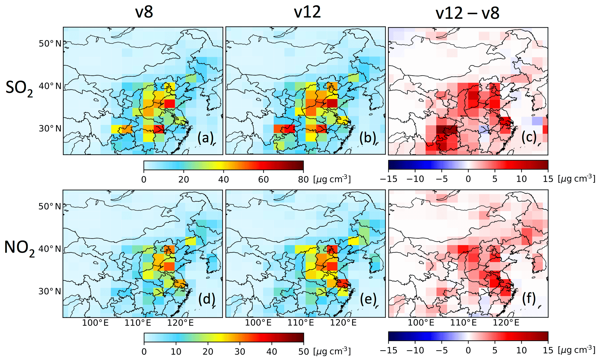
Figure 1 Simulations of surface SO₂ and NO₂ concentrations for October 2013. Panels (a) and (b) show surface SO₂ simulated by GC adjoint v35m (developed based on GEOS-Chem version 8.2.1, updated through version 9, and we name it v8 for short) and GCv12.0.0 (v12 for short), respectively, and (c) shows the difference between v12 and v8. Panels (d)–(f) are similar to (a)–(c) but for NO₂.

3.2 Downscaling GEOS-Chem surface concentrations

GEOS-Chem surface SO₂ and NO₂ concentrations at a resolution of $\mathrm{2}{}^{\circ }\times \mathrm{2.5}{}^{\circ }$ are not expected to be able to capture hot spots due to the CGS effect, and thus we aim to downscale them to finer resolutions. The prior emissions are MIX for October and November 2010. The posterior emissions are from separate inverse emission estimates in Part 1 (e.g., E−SO₂ and E−NO₂ experiments as described in Wang et al., 2020), unless it is specifically stated. The downscaling methods here should be distinguished from interpolation approaches to simply increasing spatial resolutions.

3.2.1 Downscaling concentrations with MIX simulations

With the assumption that surface concentrations of GEOS-Chem simulations using outdated emissions have correct spatial distributions at fine scales but systemic bias at coarse scales, we use $\mathrm{0.25}{}^{\circ }\times \mathrm{0.3125}{}^{\circ }$ prior surface concentration patterns to downscale both prior and posterior $\mathrm{2}{}^{\circ }\times \mathrm{2.5}{}^{\circ }$ simulations of surface species concentrations as shown in Eq. (1).

$$\begin{array}{}\text{(1)}& C_{f,i}^{\mathrm{MIX}-\mathrm{DDC}}=C_{\mathrm{c}}\times {\displaystyle \frac{C_{f,i}^{\mathrm{pri}}}{\frac{\mathrm{1}}{n}\times {\sum }_{i=\mathrm{1}}^n{C}_{f,i}^{\mathrm{pri}}}}\end{array}$$

A coarse $\mathrm{2}{}^{\circ }\times \mathrm{2.5}{}^{\circ }$ grid cell consists of n (64) fine $\mathrm{0.25}{}^{\circ }\times \mathrm{0.3125}{}^{\circ }$ grid cells, and $C_{f,i}^{\mathrm{pri}}$ represents the MIX prior simulation of surface concentrations from the ith $\mathrm{0.25}{}^{\circ }\times \mathrm{0.3125}{}^{\circ }$ grid cell within a $\mathrm{2}{}^{\circ }\times \mathrm{2.5}{}^{\circ }$ grid cell. Thus, $\frac{\mathrm{1}}{n}\times {\sum }_{i=\mathrm{1}}^n{C}_{f,i}^{\mathrm{pri}}$ is the mean $\mathrm{0.25}{}^{\circ }\times \mathrm{0.3125}{}^{\circ }$ simulation in a $\mathrm{2}{}^{\circ }\times \mathrm{2.5}{}^{\circ }$ grid cell, and $\frac{C_{f,i}^{\mathrm{pri}}}{\frac{\mathrm{1}}{n}\times {\sum }_{i=\mathrm{1}}^n{C}_{f,i}^{\mathrm{pri}}}$ is the mass ratio between fine and coarse grids, which multiples the $\mathrm{2}{}^{\circ }\times \mathrm{2.5}{}^{\circ }$ surface concentration, C_c, to obtain the downscaled result $C_{f,i}^{\mathrm{MIX}-\mathrm{DDC}}$. This approach is referred to as dynamic downscaling concentration with MIX simulation (MIX-DDC). Here, dynamic downscaling means the application of fine-scale model concentrations to downscale coarse-resolution concentrations.

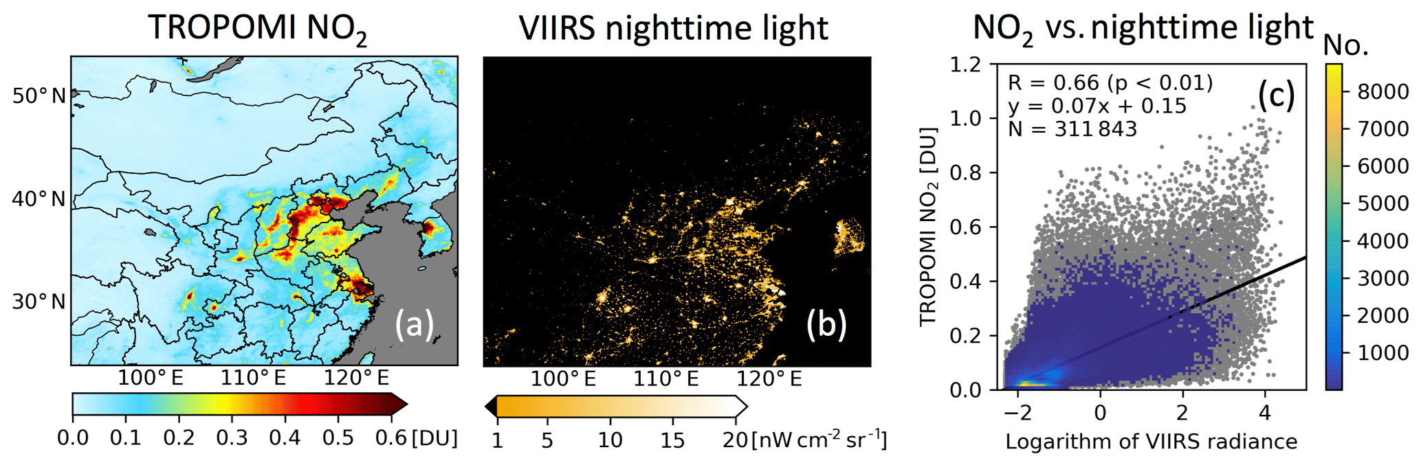
Figure 2 Panels (a) and (b) show TROPOMI NO₂ VCD and VIIRS nighttime light radiance at the $\mathrm{0.05}{}^{\circ }\times \mathrm{0.05}{}^{\circ }$ resolution in April 2018. Panel (c) shows a scatter plot of TROPOMI NO₂ versus the logarithm of VIIRS nighttime light radiance (grid cells with VIIRS nighttime light radiance less than 0.1 nW cm⁻² sr⁻¹ are removed).

3.2.2 Downscaling concentrations with nighttime lights

The VIIRS nighttime lights product at a resolution of $\mathrm{0.05}{}^{\circ }\times \mathrm{0.05}{}^{\circ }$ is used to downscale GEOS-Chem simulations of surface NO₂ due to its high spatial resolution and strong correlation with population distribution (Bennett and Smith, 2017) as well as NO₂ VCDs. Figure 2a–b show the spatial distributions of VIIRS nighttime lights and TROPOMI NO₂ tropospheric VCDs over China, and it is not surprising that both nighttime lights and NO₂ hot spots are mainly over metropolises. Figure 2c shows a strong linear correlation between the logarithm of VIIRS nighttime lights and TROPOMI NO₂ tropospheric VCDs at a resolution of $\mathrm{0.05}{}^{\circ }\times \mathrm{0.05}{}^{\circ }$. This strong correlation is because (1) nighttime lights are a good spatial proxy for allocating NO_x emissions (Geng et al., 2017); and (2) NO₂ lifetime is short (several hours), which means the distribution of NO₂ concentration hot spots is highly affected by source locations. This relationship is used to downscale as shown in Eq. (2) and (3).

$$\begin{array}{}\text{(2)}& {\displaystyle }& {\displaystyle }{W}_i=\ln \left(V_i\right)-\ln \left(\mathrm{0.1}\right)\text{(3)}& {\displaystyle }& {\displaystyle }{C}_{f,i}^{\mathrm{NL}-\mathrm{DC}}=C_{\mathrm{c}}\times {\displaystyle \frac{W_i}{\stackrel{\mathrm{‾}}{W}}}\end{array}$$

V_i represents the i VIIRS $\mathrm{0.05}{}^{\circ }\times \mathrm{0.05}{}^{\circ }$ nighttime light in a $\mathrm{2}{}^{\circ }\times \mathrm{2.5}{}^{\circ }$ grid cell, and all nighttime lights less than 0.1 nW cm⁻² sr⁻¹ are set to be 0.1 nW cm⁻² sr⁻¹; thus, the minimum of W_i is naught. $\stackrel{\mathrm{‾}}{W}$ is the average of W_i in a $\mathrm{2}{}^{\circ }\times \mathrm{2.5}{}^{\circ }$ grid cell, and we assume $W_i/\stackrel{\mathrm{‾}}{W}$ represents the ratio of the surface NO₂ concentration at $\mathrm{0.05}{}^{\circ }\times \mathrm{0.05}{}^{\circ }$ to that at $\mathrm{2}{}^{\circ }\times \mathrm{2.5}{}^{\circ }$, due to the relationship between VIIRS nighttime lights and TROPOMI NO₂ tropospheric VCDs. The ratio multiplies the surface NO₂ concentration at $\mathrm{2}{}^{\circ }\times \mathrm{2.5}{}^{\circ }$ C_c to obtain the downscaled result $C_{f,i}^{\mathrm{NL}-\mathrm{DC}}$. This approach is referred to as nighttime light downscaling concentration (NL-DC).

We do not expect that this approach can be used to downscale SO₂ concentrations because (1) nighttime lights are not a very good spatial proxy for allocating SO₂ emissions as SO₂ emissions from traffic sector are very small, while nighttime lights are strong over rush traffic road; and (2) SO₂ lifetime is 1–2 d, which is much longer than NO₂ lifetime.

3.3 Downscaling emissions

To simulate or forecast surface SO₂ and NO₂ concentrations at a resolution of $\mathrm{0.25}{}^{\circ }\times \mathrm{0.3125}{}^{\circ }$ through the GEOS-Chem model, the posterior emissions at a resolution of $\mathrm{2}{}^{\circ }\times \mathrm{2.5}{}^{\circ }$ should be downscaled to fit the model resolution. The prior MIX 2010 emission inventory has a spatial resolution of $\mathrm{0.25}{}^{\circ }\times \mathrm{0.25}{}^{\circ }$, which is slightly finer than $\mathrm{0.25}{}^{\circ }\times \mathrm{0.3125}{}^{\circ }$, and it can be easily processed to fit $\mathrm{0.25}{}^{\circ }\times \mathrm{0.3125}{}^{\circ }$ simulations through HEMCO – the GEOS-Chem emission processing package (Keller et al., 2014). Thus, all the posterior emissions at a resolution of $\mathrm{2}{}^{\circ }\times \mathrm{2.5}{}^{\circ }$ are downscaled to $\mathrm{0.25}{}^{\circ }\times \mathrm{0.25}{}^{\circ }$, which are further regridded to $\mathrm{0.25}{}^{\circ }\times \mathrm{0.3125}{}^{\circ }$ with HEMCO. We introduce two emission downscaling approaches with prior MIX $\mathrm{0.25}{}^{\circ }\times \mathrm{0.25}{}^{\circ }$ emissions and $\mathrm{0.05}{}^{\circ }\times \mathrm{0.05}{}^{\circ }$ VIIRS nighttime lights used as spatial proxies. The two methods are referred to as downscaling emissions with MIX (MIX-DE) and downscaling emissions with nighttime light (NL-DE).

3.3.1 MIX-DE

We assume fine-resolution prior emission inventories have correct relative spatial distributions at fine scales, but a systemic bias exists at coarse scales. The emission downscaling approach is shown in Eq. (4), where $E_{f,i}^{\mathrm{pri}}$ is the ith MIX emission estimate at $\mathrm{0.25}{}^{\circ }\times \mathrm{0.25}{}^{\circ }$ resolution in a $\mathrm{2}{}^{\circ }\times \mathrm{2.5}{}^{\circ }$ grid cell for year 2010, n(=80) is the number of $\mathrm{0.25}{}^{\circ }\times \mathrm{0.25}{}^{\circ }$ grids in a $\mathrm{2}{}^{\circ }\times \mathrm{2.5}{}^{\circ }$ grid cell, $E_{\mathrm{c}}^{\mathrm{post}}$ is posterior emissions at $\mathrm{2}{}^{\circ }\times \mathrm{2.5}{}^{\circ }$ from Wang et al. (2020), and $E_{f,i}^{\mathrm{MIX}-\mathrm{DE}}$ is the downscaled posterior emissions at $\mathrm{0.25}{}^{\circ }\times \mathrm{0.25}{}^{\circ }$ resolution.

$$\begin{array}{}\text{(4)}& E_{f,i}^{\mathrm{MIX}-\mathrm{DE}}=E_{\mathrm{c}}^{\mathrm{post}}\times {\displaystyle \frac{E_{f,i}^{\mathrm{pri}}}{{\sum }_{i=\mathrm{1}}^n{E}_{f,i}^{\mathrm{pri}}}}\end{array}$$

Figure 3 Panels (a) and (b) show VIIRS nighttime light radiance and MIX NO_x emissions at $\mathrm{0.25}{}^{\circ }\times \mathrm{0.25}{}^{\circ }$ resolution in April 2018 and April 2010, respectively. Panel (c) shows a scatter plot of MIX NO_x emissions versus VIIRS nighttime light radiance (grid cells with VIIRS nighttime light radiance less than 0.1 nW cm⁻² sr⁻¹ are removed).

3.3.2 NL-DE

VIIRS nighttime lights are good proxies for allocating CO₂ emissions (Ou et al., 2015), and they are also expected to be useful for downscaling NO_x emissions. Figure 3 shows that VIIRS nighttime lights and MIX NO_x emissions have similar spatial patterns, and the linear correlation coefficient between them is as high as 0.73. Thus, VIIRS nighttime lights at a resolution of $\mathrm{0.05}{}^{\circ }\times \mathrm{0.05}{}^{\circ }$ are used to downscale NO_x emissions as shown in Eq. (5). $E_{\mathrm{c}}^{\mathrm{post}}$ represents posterior emissions at $\mathrm{2}{}^{\circ }\times \mathrm{2.5}{}^{\circ }$ from Part 1 (Wang et al., 2020), A_i and V_i are the ith area and VIIRS nighttime lights at $\mathrm{0.05}{}^{\circ }\times \mathrm{0.05}{}^{\circ }$, respectively, and n(=2000) is the number of $\mathrm{0.05}{}^{\circ }\times \mathrm{0.05}{}^{\circ }$ grids in a $\mathrm{2}{}^{\circ }\times \mathrm{2.5}{}^{\circ }$ grid cell. $E_{f,i}^{\mathrm{NL}-\mathrm{DE}}$ is the downscaled posterior NO_x emissions at $\mathrm{0.05}{}^{\circ }\times \mathrm{0.05}{}^{\circ }$, which is further aggregated to $\mathrm{0.25}{}^{\circ }\times \mathrm{0.25}{}^{\circ }$.

$$\begin{array}{}\text{(5)}& E_{f,i}^{\mathrm{NL}-\mathrm{DE}}=E_{\mathrm{c}}^{\mathrm{post}}\times {\displaystyle \frac{A_i{V}_i}{{\sum }_{i=\mathrm{1}}^n{A}_i{V}_i}}\end{array}$$

Table 1 Design of experiments for simulating surface SO₂ and NO₂ concentrations over China in October 2013.

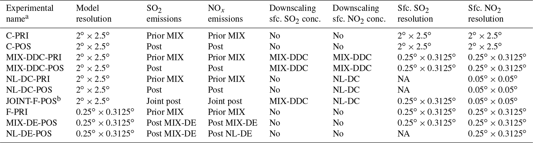
^a The nomenclature of the experimental name is as follows. C: coarse resolution, F: fine resolution, PRI: prior, POS: posterior, DDC: dynamic downscaling concentration, DC: downscaling concentration, NL: nighttime light, MIX: prior MIX emission inventory, DE: downscaling emissions, JOINT: emission inventory from joint inverse modeling. ^b JOINT-F-POS is a set of experiments using posterior emission inventories from joint inversion modeling using a different observation balance parameter γ.

3.4 Design of experiments

3.4.1 Simulations for October 2013

A set of GEOS-Chem simulation experiments are designed to illustrate the impacts of model resolutions and emission inventories on simulating surface SO₂ and NO₂ concentrations over China for October 2013, as summarized in Table 1. Simulations of surface SO₂ and NO₂ concentrations are evaluated with in situ observations. C-PRI and C-POS are designed to show the CGS effect of surface SO₂ and NO₂ concentrations in coarse (C-) resolution simulations with prior (PRI) and posterior (POS) emissions, respectively. Both C-PRI and C-POS have a simulation resolution of $\mathrm{2}{}^{\circ }\times \mathrm{2.5}{}^{\circ }$ and use the prior and posterior emissions, respectively. MIX-DDC-PRI, MIX-DDC-POS, NL-DC-PRI, and NL-DC-POS illustrate alleviation of the CGS effect through downscaling of surface concentrations. In MIX-DDC-PRI and MIX-DDC-POS, surface SO₂ and NO₂ concentrations at $\mathrm{2}{}^{\circ }\times \mathrm{2.5}{}^{\circ }$ from C-PRI and C-POS are downscaled to the resolution of $\mathrm{0.25}{}^{\circ }\times \mathrm{0.3125}{}^{\circ }$ through the MIX-DDC approach. NL-DC-PRI and NL-DC-POS downscale NO₂ concentrations at $\mathrm{2}{}^{\circ }\times \mathrm{2.5}{}^{\circ }$ from C-PRI and C-POS to the resolution of $\mathrm{0.05}{}^{\circ }\times \mathrm{0.05}{}^{\circ }$ through the NL-DC approach. JOINT-F-POS is designed to show the impacts of using posterior emissions from joint (JOINT) assimilations on surface SO₂ and NO₂ forecast at fine (F) spatial scale. In JOINT-F-POS, posterior SO₂ and NO_x emissions from joint assimilations with various observation balance parameter (γ) values from Part 1, i.e., Wang et al. (2020), are used to simulate surface SO₂ and NO₂ at $\mathrm{2}{}^{\circ }\times \mathrm{2.5}{}^{\circ }$; this parameter is used to balance the importance of the SO₂ and NO₂ observational terms in the cost function. The simulated surface SO₂ and NO₂ concentrations are further downscaled to $\mathrm{0.25}{}^{\circ }\times \mathrm{0.3125}{}^{\circ }$ through the MIX-DDC approach and $\mathrm{0.05}{}^{\circ }\times \mathrm{0.05}{}^{\circ }$ through the NL-DC approach, respectively. F-PRI, MIX-DE-POS, and NL-DE-POS illustrate the improvements when using downscaled posterior emissions to simulate surface SO₂ and NO₂ concentrations. All three simulations have a resolution of $\mathrm{0.25}{}^{\circ }\times \mathrm{0.3125}{}^{\circ }$ but use different emission inventories. F-PRI uses the prior MIX emissions, but MIX-DE-POS and NL-DE-POS use the downscaled posterior emissions. Posterior SO₂ emissions downscaled through the MIX-DE approach are used in the two simulations, but posterior NO_x emissions used in MIX-DE-POS and NL-DE-POS are downscaled through the MIX-DE and NL-DE approaches, respectively.

Table 2 Design of experiments for forecasting surface SO₂, NO₂, and O₃ concentrations over China in November 2013.

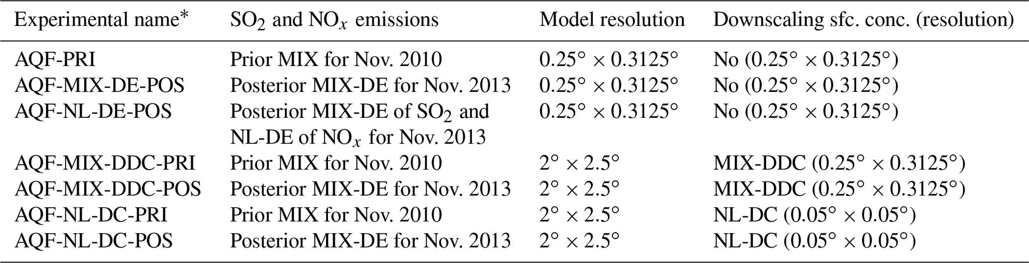
^* The nomenclature of the experimental name is as follows. AQF: air quality forecasts, PRI: prior, POS: posterior, MIX: prior MIX emission inventory, NL: nighttime light, DE: downscaling emissions, DDC: dynamic downscaling concentration, DC: downscaling concentration.

3.4.2 Forecasts for November 2013

Y. Wang et al. (2016) used posterior emissions of the current month to improve air quality forecasts of the next month. We implement a similar approach in this study, but emission variations among different months are also considered. With the assumption that the prior MIX emission inventory has proper temporal variations among different months, posterior MIX-DE and NL-DE emission inventories for November 2013 are obtained by multiplying posterior MIX-DE or NL-DE emission inventories for October 2013, respectively, by the ratios of prior MIX emissions between November and October 2010. As summarized in Table 2, we design a set of experiments for air quality forecasts (AQFs) of surface SO₂, NO₂, and O₃ concentrations at fine resolution over China in November 2013. AQF-PRI uses the prior MIX inventory for November 2010 to forecast surface SO₂, NO₂, and O₃ concentrations of November 2013 at $\mathrm{0.25}{}^{\circ }\times \mathrm{0.3125}{}^{\circ }$, while AQF-MIX-DE-POS uses the posterior MIX-DE inventory for November 2013. AQF-NL-DE-POS is similar to AQF-MIX-DE-POS, but the posterior NL-DE inventory for NO_x is used. AQF-MIX-DDC-PRI and AQF-MIX-DDC-POS use the prior MIX for November 2010 and posterior MIX-DE for November 2013 inventories to forecast surface SO₂ and NO₂ concentrations at $\mathrm{2}{}^{\circ }\times \mathrm{2.5}{}^{\circ }$, which are further downscaled to $\mathrm{0.25}{}^{\circ }\times \mathrm{0.3125}{}^{\circ }$ through the MIX-DDC approach. Since NO₂ hot spots cannot be captured at $\mathrm{0.25}{}^{\circ }\times \mathrm{0.3125}{}^{\circ }$ resolution, the NL-DC approach is also applied to the NO₂ forecasts. Thus, AQF-NL-DC-PRI and AQF-NL-DC-POS use the prior MIX inventory for November 2010 and the posterior MIX-DE inventory for November 2013 to forecast surface SO₂ and NO₂ concentrations of November 2013 at $\mathrm{2}{}^{\circ }\times \mathrm{2.5}{}^{\circ }$, which are further downscaled to $\mathrm{0.05}{}^{\circ }\times \mathrm{0.05}{}^{\circ }$ according to VIIRS nighttime light of October 2013 through the NL-DC approach.

3.5 Evaluation statistics

We use the linear correlation coefficient (R), mean bias (MB), normalized mean bias (NMB), normalized centered root mean square error (NCRMSE) (Wang et al., 2020), and normalized mean squared error (NMSE) as measures to evaluate GEOS-Chem SO₂ and NO₂ surface concentrations with in situ observations. NCRMSE measures the spatial distribution difference between forecasts, and in situ observations are similar to the root mean squared error, but the impact of bias is removed. NMSE is defined as Eq. (6), where M_i and O_i are the ith GEOS-Chem simulation and in situ observation, respectively, $\stackrel{\mathrm{‾}}{O}$ is mean of the observations, and N is number of the observations.

$$\begin{array}{}\text{(6)}& \mathrm{NMSE}={\displaystyle \frac{\frac{\mathrm{1}}{N}{\sum }_{i=\mathrm{1}}^N(M_i-O_i{)}^{\mathrm{2}}}{\frac{\mathrm{1}}{N}{\sum }_{i=\mathrm{1}}^N(O_i-\stackrel{\mathrm{‾}}{O}{)}^{\mathrm{2}}}}\end{array}$$

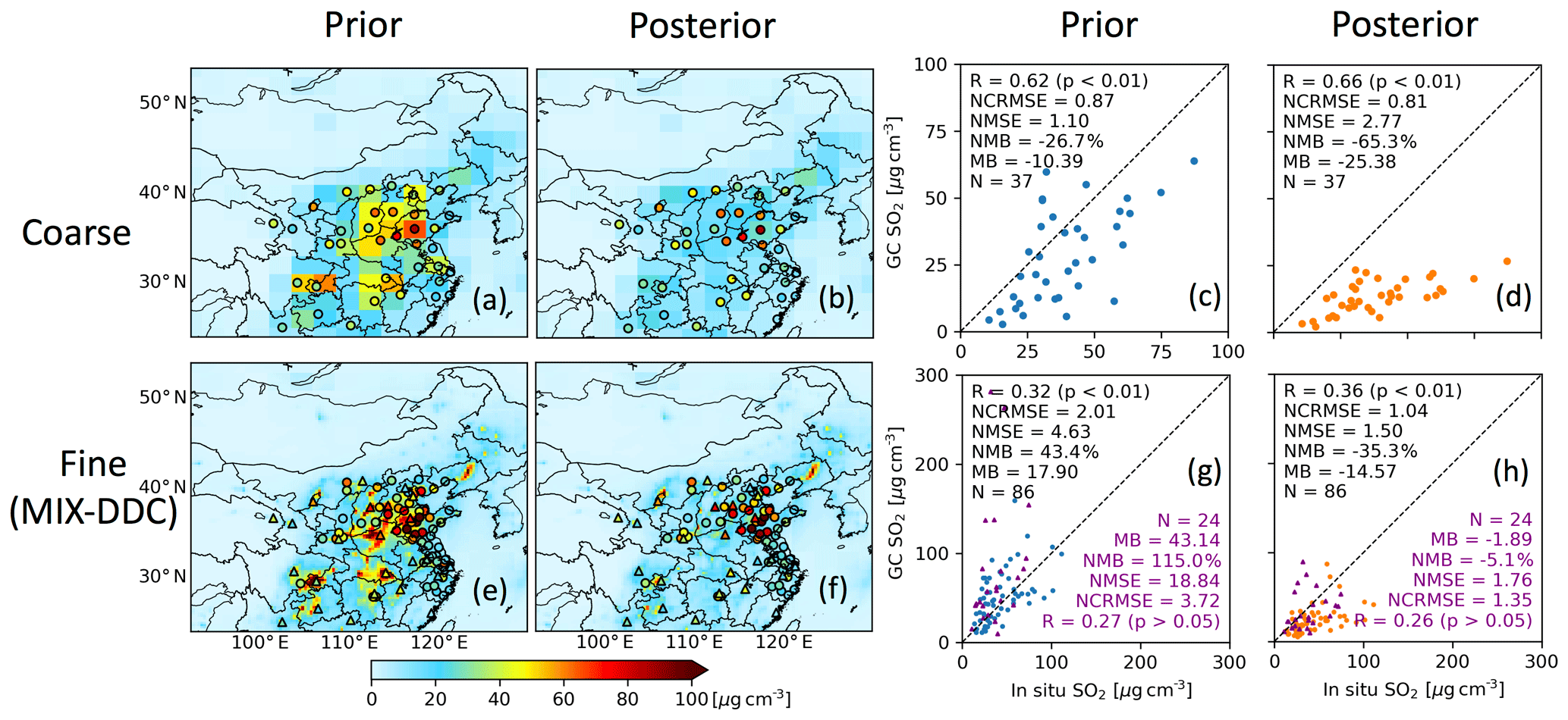
Figure 4 Evaluations of coarse-resolution, MIX-DDC GEOS-Chem surface SO₂ simulations with in situ observations for October 2013. Panels (a) and (b) show C-PRI and C-POS simulations, respectively, with in situ observations overlapped. If there is more than one observation in a $\mathrm{2}{}^{\circ }\times \mathrm{2.5}{}^{\circ }$ grid cell, they are averaged. Panels (c) and (d) show scatter plots of C-PRI and C-POS simulations versus in situ observations, respectively. Panels (e) and (f) show surface SO₂ concentrations of MIX-DDC-PRI and MIX-DDC-POS, respectively, with in situ province-capital-city (triangle) and non-province-capital-city (circle) observations overlapped. Panels (g) and (h) show scatter plots of MIX-DDC-PRI and MIX-DDC-POS simulations versus in situ province-capital-city (triangle) and non-province-capital-city (circle) observations, respectively. The linear correlation coefficient (R), normalized centered root mean squared error (NCRMSE), normalized mean squared error (NMSE), normalized mean bias (NMB), mean bias (MB), and number of observations (N) are shown over scatter plots, with black color text for all observations and purple color text for province-capital-city observations.

4 Results

4.1 CGS and MIX-DDC for SO₂

The CGS effect of surface SO₂ concentrations in the coarse-resolution ($\mathrm{2}{}^{\circ }\times \mathrm{2.5}{}^{\circ }$) simulations (C-PRI and C-POS experiments) is shown in Fig. 4a–d. The GEOS-Chem $\mathrm{2}{}^{\circ }\times \mathrm{2.5}{}^{\circ }$ simulation of every grid cell is the average of surface SO₂ at $\sim \mathrm{5}\times {\mathrm{10}}^{\mathrm{4}}$ km² area, while in situ SO₂ observations can only represent average concentrations of a much smaller area. Considering that all sites are in cities, where emission sources are located, GEOS-Chem $\mathrm{2}{}^{\circ }\times \mathrm{2.5}{}^{\circ }$ simulations are expected to be smaller than in situ observations. In this study, the NMB is −26.7 % (Fig. 4c) in the C-PRI simulation, while the C-POS simulation shows an even stronger negative NMB of bias of −65.3 % (Fig. 4d), as the posterior SO₂ emission is 35.8 % smaller than prior MIX 2010.

To decrease the impact of CGS on surface SO₂ simulations, both the prior and posterior GEOS-Chem surface SO₂ simulations at $\mathrm{2}{}^{\circ }\times \mathrm{2.5}{}^{\circ }$ resolution are downscaled to $\mathrm{0.25}{}^{\circ }\times \mathrm{0.3125}{}^{\circ }$ through the MIX-DDC approach (MIX-DDC-PRI and MIX-DDC-POS experiments). Zheng et al. (2017) showed that surface SO₂ concentration simulations from WRF-CMAQ, when evaluating with in situ observations, have a NMB of −23 %, 7 %, and 41 % at the resolutions of 36 km (∼ 0.36^∘), 12 km (∼ 0.12^∘), and 4 km (∼ 0.04^∘), respectively, which suggests that (1) the CGS effect and other nonlinear resolution-dependent processes can affect SO₂ simulation results and (2) these problems are alleviated at the resolution of $\mathrm{0.25}{}^{\circ }\times \mathrm{0.3125}{}^{\circ }$ but are not completely avoided. The downscaled prior (MIX-DDC-PRI) and posterior (MIX-DDC-POS) GEOS-Chem surface SO₂ concentrations at $\mathrm{0.25}{}^{\circ }\times \mathrm{0.3125}{}^{\circ }$ are shown in Fig. 4e–h. MIX-DDC-PRI and MIX-DDC-POS SO₂ simulations show hot spots of up to 270 µg m⁻³ (Fig. 4e) and 80 µg m⁻³ (Fig. 4f), respectively, compared with the largest value of less than 60 µg m⁻³ (Fig. 4a) and 35 µg m⁻³ (Fig. 4b) in the C-PRI and C-POS simulations, respectively.

MIX-DDC-POS SO₂ simulations are in better agreement with in situ observations than MIX-DDC-PRI. The NMSE decreases from 4.63 in MIX-DDC-PRI to 1.50 in MIX-DDC-POS, and the linear correlation coefficient (R) increases from 0.32 to 0.36 (Fig. 4g–h). The NMB changes, however, from 43.4 % to −35.3 % (Fig. 3g–h), which implies the CGS effect may not be completely avoided at a resolution of $\mathrm{0.25}{}^{\circ }\times \mathrm{0.3125}{}^{\circ }$, and other factors that may affect the result should be investigated in the future. We also separately compare MIX-DDC-PRI and MIX-DDC-POS simulations with in situ observations over provincial capital cities, as SO₂ hot spots in smaller cities may still be difficult to capture using the $\mathrm{0.25}{}^{\circ }\times \mathrm{0.3125}{}^{\circ }$ MIX-DDC-PRI and MIX-DDC-POS simulations. The NMB is 115.0 % in the MIX-DDC-PRI simulation and reduces to −5 % in the MIX-DDC-POS simulation. Additionally, the MIX-DDC-POS simulation shows better spatial pattern than the MIX-DDC-PRI simulation in terms of NCRMSE, although linear correlation decreases slightly. In spite of the improvement of capturing hot spots in term of NMB using the MIX-DDC approach, we should also note that the coarse-resolution simulations (Fig. 4c, d) have larger linear correlation coefficients and smaller NCRMSEs than the MIX-DDC simulations. Thus, for SO₂ simulations, MIX-DDC helps to capture hot spots but can make the spatial distribution worse than the original coarse-resolution simulations in terms of NCRMSE. The spatial pattern degradation implies that current chemistry transport simulations of surface SO₂ concentrations can capture the regional spatial pattern (coarse resolution) well, but it is difficult to simulate the local spatial pattern (fine resolution); the weakness for describing the local spatial pattern simulation suggests the uncertainties of either bottom-up SO₂ emission estimates at fine resolution or locally resolved meteorological fields (Ge et al., 2017), or both. This uncertainty in bottom-up emission inventories can further stem from distributing SO₂ emissions at the provincial level to a fine-resolution grid. MIX-DDC also performs well when GC adjoint v35m is used for coarse resolution, and results show better spatial pattern (smaller NCRMSE) than using GC v12.0.0 (Fig. S2).

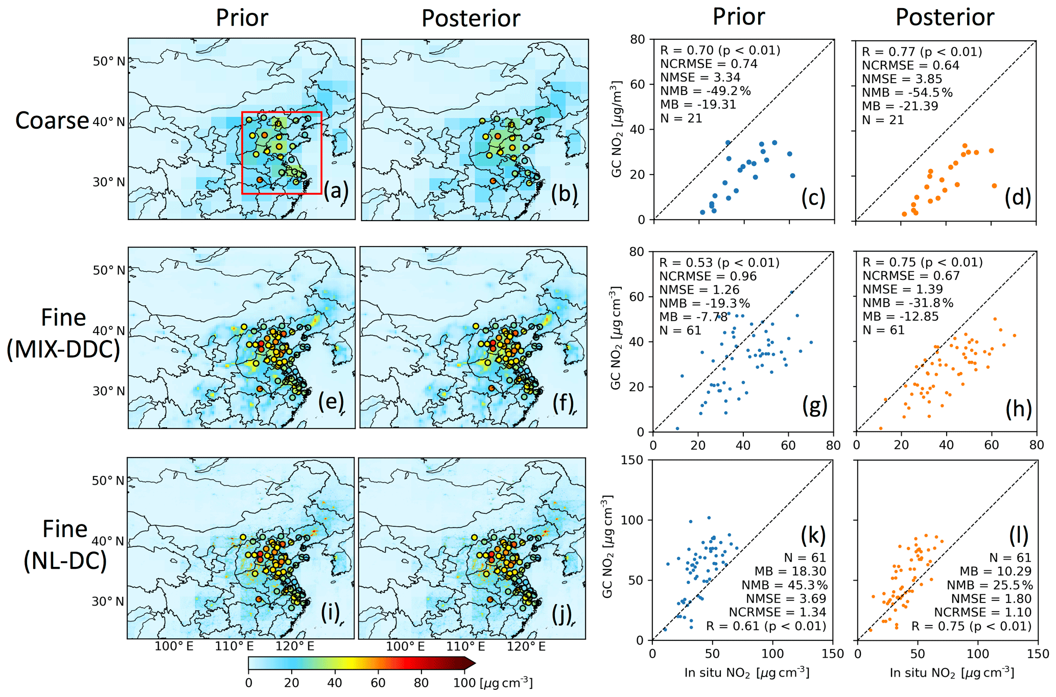
Figure 5 Evaluation of coarse-resolution, MIX-DDC, and NL-DC GEOS-Chem surface NO₂ simulations with in situ observations for October 2013. Panels (a) and (b) show C-PRI and C-POS simulations, respectively, with in situ observations overlapped. If there is more than one observation in a $\mathrm{2}{}^{\circ }\times \mathrm{2.5}{}^{\circ }$ grid cell, they are averaged. Panels (c) and (d) show scatter plots of C-PRI and C-POS simulations versus in situ observations, respectively. Panels (e) and (f) show GEOS-Chem surface NO₂ of MIX-DDC-PRI and MIX-DDC-POS, respectively, with in situ observations overlapped. Panels (g) and (h) show scatter plots of MIX-DDC-PRI and MIX-DDC-POS simulations versus in situ observations, respectively. Panels (i)–(l) are similar to (e)–(h), respectively, but results are downscaled through the NL-DC approach (NL-DC-PRI and NL-DC-POS). The linear correlation coefficient (R), normalized centered root mean squared error (NCRMSE), normalized mean squared error (NMSE), normalized mean bias (NMB), mean bias (MB), and number of observations (N) are shown over scatter plots. As NO_x emission is mainly over the North China Plain and eastern China, validation with in situ surface NO₂ is conducted at these areas (red box in a).

4.2 CGS, MIX-DDC, and NL-DC for NO₂

NO₂ has an even shorter lifetime than SO₂; thus the CGS effect also exists in the C-PRI and C-POS simulations. Figure 5a–d show that almost all in situ NO₂ observations are larger than the GEOS-Chem simulations, regardless of whether the prior MIX 2010 (C-PRI) or the posterior (C-POS) NO_x emissions are used. GEOS-Chem surface NO₂ averages from the C-PRI and C-POS simulations, sampled according to in situ observational sites, are 49.2 % and 54.5 % smaller than the average of in situ observations, respectively.

The MIX-DDC approach is also applied to downscale NO₂ surface simulations (MIX-DDC-PRI and MIX-DDC-POS experiments), and the results are evaluated with in situ observations. As discussed, according to Zheng et al. (2017), the CGS effect and other nonlinear resolution-dependent problems can be alleviated at the resolution of $\mathrm{0.25}{}^{\circ }\times \mathrm{0.3125}{}^{\circ }$ (such as in MIX-DDC-PRI and MIX-DDC-POS experiments) but cannot be completely avoided. The MIX-DDC-POS simulation is better than the MIX-DDC-PRI simulation in terms of spatial pattern (NCRMSE), although the CGS effect may still exists and other nonlinear resolution-dependent problem should be investigated in the future. The NMB is −19.3 % and −31.8 % for the MIX-DDC-PRI and MIX-DDC-POS simulations, respectively (Fig. 5e–h), which implies that $\mathrm{0.25}{}^{\circ }\times \mathrm{0.3125}{}^{\circ }$ may be still too coarse to capture hot spots due to the short lifetime of NO₂. The larger negative bias in the MIX-DDC-POS simulation than in the MIX-DDC-PRI also leads to the former showing large NMSE. Despite the negative bias, R between observations and the MIX-DDC simulations increases from 0.53 in MIX-DDC-PRI to 0.75 in MIX-DDC-POS, and the NCRMSE reduces from 0.96 to 0.67, which is only slightly larger than 0.64 in the C-POS simulation. Thus MIX-DDC-POS can better capture NO₂ hot spots and shows spatial pattern as good as C-POS. MIX-DDC also performs well when GC adjoint v35m is used for coarse-resolution simulations, and results show better spatial pattern (smaller NCRMSE) than using GC v12.0.0 (Fig. S3).

To further alleviate the CGS effect, we downscale GEOS-Chem surface NO₂ simulations at $\mathrm{2}{}^{\circ }\times \mathrm{2.5}{}^{\circ }$ to $\mathrm{0.05}{}^{\circ }\times \mathrm{0.05}{}^{\circ }$ according to VIIRS nighttime light distributions through the NL-DC approach (NL-DC-PRI and NL-DC-POS experiments), and the results are evaluated with in situ surface NO₂ observations (Fig. 5i–l). The largest GEOS-Chem surface NO₂ values are less than 35 µg m⁻³ in both the coarse C-PRI and C-POS simulations (Fig. 5a, b), while they are larger than 100 µg m⁻³ at $\mathrm{0.05}{}^{\circ }\times \mathrm{0.05}{}^{\circ }$ in the NL-DC-PRI and NL-DC-POS simulations (Fig. 5i, j). The scatter plots of the NL-DC-PRI (Fig. 5k) and NL-DC-POS (Fig. 5l) simulations versus in situ surface NO₂ observations show that R increases from 0.61 in the NL-DC-PRI simulation to 0.75 in the NL-DC-POS simulation, and NMSE decreases from 3.69 to 1.80, which is smaller than that in the coarse-resolution simulations and the MIX-DDC downscaled simulation. It suggests that NL-DC has the advantage of downscaling surface concentrations (without evoking any CTM simulation and its associated needs of computational resources). The biases of surface NO₂ concentrations are 45.3 % and 25.5 % for NL-DC-PRI and NL-DC-POS, respectively, which could come from total emission bias as well as the downscaling process through the NL-DC approach. The sites used for validation are mainly over urban regions, and we lack sites that are located over rural regions to evaluate if positive or negative bias persists over rural regions. Thus, we are not able to determine how much of the positive bias in NL-DC-PRI and NL-DC-POS is caused by the NL-DC approach. When NL-DC is applied to downscale GC adjoint v35m coarse-resolution simulations, results show better spatial pattern (smaller NCRMSE) than that of GC v12.0.0 (Fig. S3).

The surface NO₂ concentrations used for evaluation are derived from measurements of (NO₂)_m assuming r${}_{{\mathrm{NO}}_{\mathrm{2}}}$ of 0.83 as stated in Sect. 2.1. Due to the lack of information on r${}_{{\mathrm{NO}}_{\mathrm{2}}}$, we also test the values in the range of 0.7 to 1.0, and the derived NO₂ concentrations are used to validate the NL-DC-PRI and NL-DC-POS simulations at the $\mathrm{0.05}{}^{\circ }\times \mathrm{0.05}{}^{\circ }$ resolution. Figure 6 shows that the NL-DC-POS simulation has NMSE in the range of 1 to 4, which is always better than the NL-DC-PRI simulation with NMSE in the range of 2 to 8.

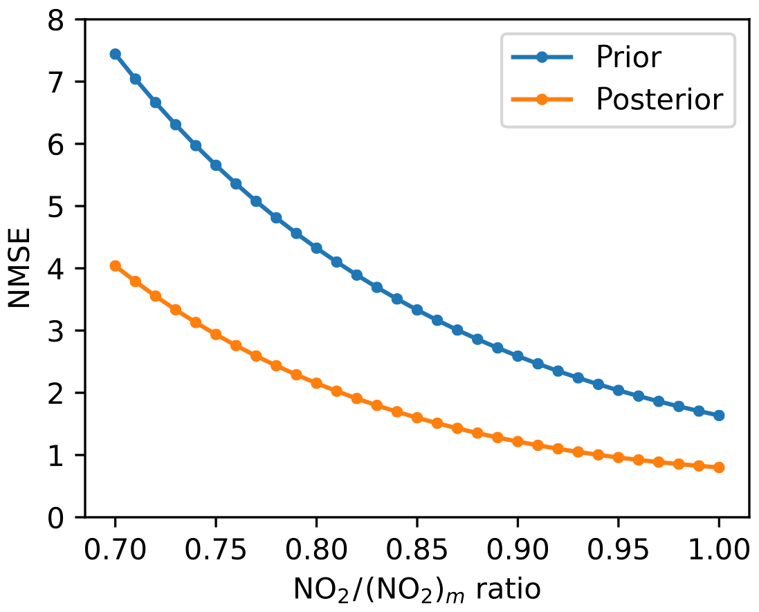
Figure 6 Normalized mean squared error (NMSE) for NL-DC-PRI (blue line) and NL-DC-POS (orange line) when evaluating with in situ surface NO₂ derived from various NO₂∕(NO₂)_m ratios (increasing from 0.7 to 1.0 with a step of 0.01), where (NO₂)_m is measured NO_z concentration.

Figure 7 Panel (a) shows SO₂ $\mathrm{0.25}{}^{\circ }\times \mathrm{0.3125}{}^{\circ }$ emissions of prior MIX 2010, (b) shows posterior MIX-DE, and (c) shows the difference between posterior MIX-DE and prior MIX 2010.

4.3 MIX-DE for SO₂ simulations

Instead of downscaling simulation results as shown in Sect. 4.1, we directly simulate surface SO₂ concentrations at $\mathrm{0.25}{}^{\circ }\times \mathrm{0.3125}{}^{\circ }$ resolution through GEOS-Chem over China in October 2013 using the prior MIX 2010 emissions and the posterior emissions. The posterior SO₂ emissions at $\mathrm{2}{}^{\circ }\times \mathrm{2.5}{}^{\circ }$ resolution are downscaled to $\mathrm{0.25}{}^{\circ }\times \mathrm{0.3125}{}^{\circ }$ through the MIX-DE approach. The posterior MIX-DE SO₂ emissions are smaller than the prior MIX 2010 SO₂ emissions over northern China and southwestern China (Fig. 7).

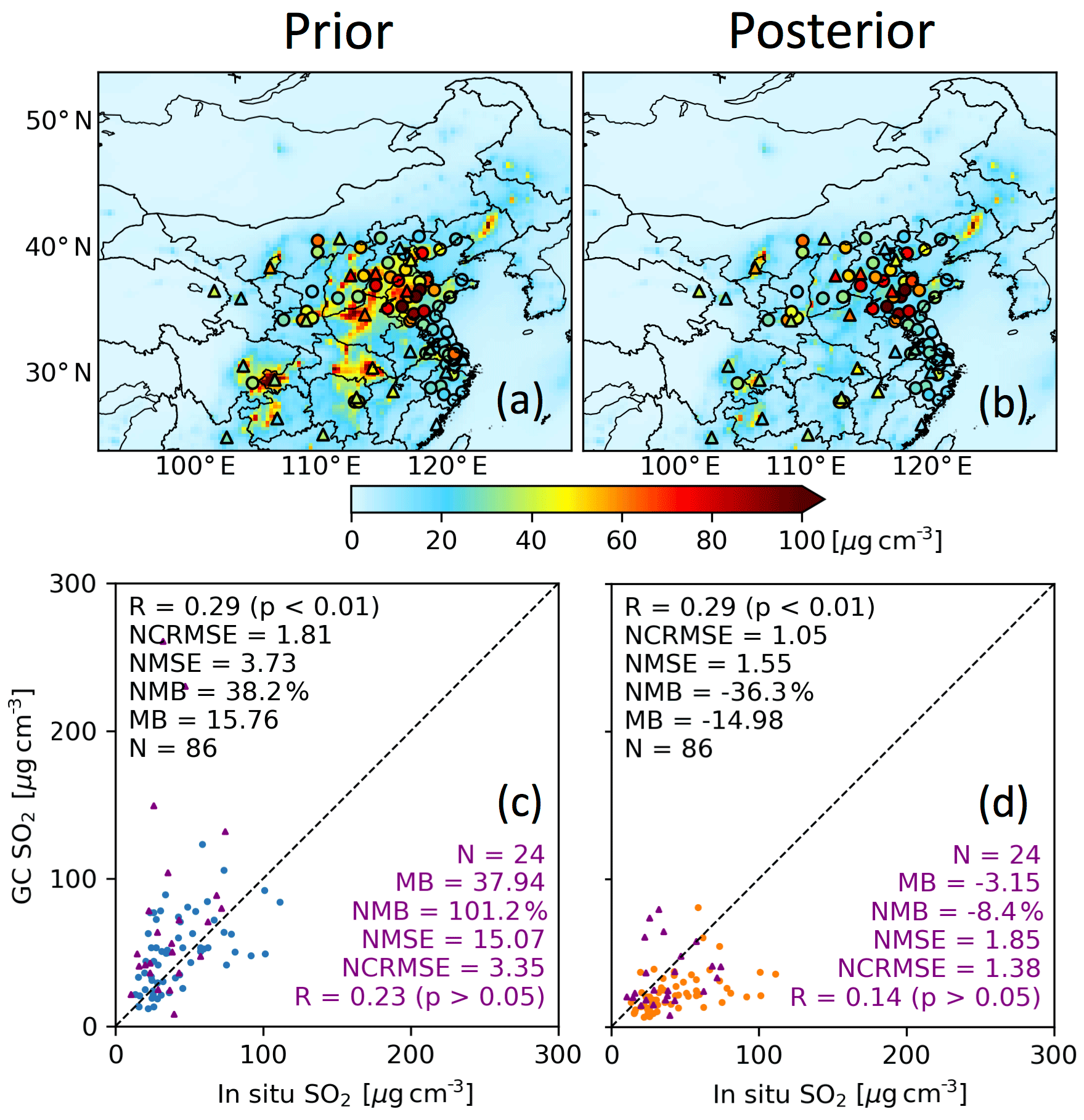
Figure 8 Evaluations of fine-resolution GEOS-Chem surface SO₂ simulations with in situ observations for October 2013. Panels (a) and (b) show surface SO₂ concentrations of F-PRI and MIX-DE-POS, respectively, with in situ province-capital-city (triangle) and non-province-capital-city (circle) observations overlapped. Panels (c) and (d) show scatter plots of F-PRI and MIX-DE-POS simulations versus in situ province-capital-city (triangle) and non-province-capital-city (circle) observations, respectively. The linear correlation coefficient (R), normalized centered root mean squared error (NCRMSE), normalized mean squared error (NMSE), normalized mean bias (NMB), mean bias (MB), and number of observations (N) are shown over scatter plots, with black color text for all observations and purple color text for province-capital-city observations.

The $\mathrm{0.25}{}^{\circ }\times \mathrm{0.3125}{}^{\circ }$ GEOS-Chem simulations of surface SO₂ for October 2013 when using the prior MIX (F-PRI experiment) and the posterior MIX-DE (MIX-DE-POS experiment) emission inventories are shown in Fig. 8. When evaluating with all in situ SO₂ observations, NMSE decreases from 3.73 in F-PRI to 1.55 in MIX-DE-POS, but bias changes from 15.76 to −14.98 µg m⁻³. For the same reason, in the MIX-DDC-PRI and MIX-DDC-POS assessment in Sect. 4.1, we also focus on provincial capital cities. In this scene, NMSE of the MIX-DE-POS simulation is 1.85 (Fig. 8d), which is much smaller than 15.07 in the F-PRI simulation (Fig. 8c), but it is slightly larger than 1.76 in the MIX-DDC-POS simulation (Fig. 4h). Moreover, NMB decreases from 101.2 % in the F-PRI simulation to −8.4 % in the MIX-DE-POS simulation (Fig. 8). R is 0.23 and 0.14 in F-PRI and MIX-DE-POS, respectively, neither of which is significant at the 95 % confidence level. In Sect. 4.2, we have shown that good spatial distribution is captured in coarse-resolution rather than fine-resolution simulations, which implies that large uncertainty of bottom-up SO₂ emission estimates at fine resolution may be introduced when distributing SO₂ emissions at the provincial level to a fine-resolution grid. It is not surprising that the correlation coefficients are small for F-PRI and MIX-DE-POS, as both are in fine resolution.

4.4 MIX-DE and NL-DE for NO₂ simulations

Posterior NO_x emissions at $\mathrm{2}{}^{\circ }\times \mathrm{2.5}{}^{\circ }$ resolution are downscaled through MIX-DE and NL-DE approaches. Figure 9 shows the prior MIX, posterior MIX-DE, and posterior NL-DE NO_x emissions at $\mathrm{0.25}{}^{\circ }\times \mathrm{0.3125}{}^{\circ }$ resolutions. All three emission inventories show NO_x emission hot spots over metropolises (Fig. 9a–c). Compared with prior MIX, posterior MIX-DE is larger over Hebei Province but smaller over most other areas of the North China Plain and eastern China (Fig. 9d). As the posterior NL-DE emission inventory is downscaled according to the VIIRS nighttime light distribution, the difference (Fig. 9e) between posterior NL-DE and prior MIX and the difference (Fig. 9f) between posterior NL-DE and posterior MIX-DE show scattered positive and negative values.

The three emission inventories are used to simulate surface NO₂ concentrations at the $\mathrm{0.25}{}^{\circ }\times \mathrm{0.3125}{}^{\circ }$ resolution over China in October 2013, that is F-PRI, MIX-DE-POS, and NL-DE-POS experiments in Table 1. All these simulations are evaluated with in situ NO₂ observations (Fig. 10). R increases from 0.46 in F-PRI to 0.61 in MIX-DE-POS and 0.58 in NL-DE-POS, and NCRMSE decreases from 0.95 in F-PRI to 0.81 in MIX-DE-POS and 0.85 in NL-DE-POS (Fig. 10d–f). Both MIX-DE-POS and NL-DE-POS show stronger negative NMB and larger NMSE than F-PRI, which should be partly caused by the CGS effect, although emission bias and other nonlinear resolution-dependent processes could play a role.

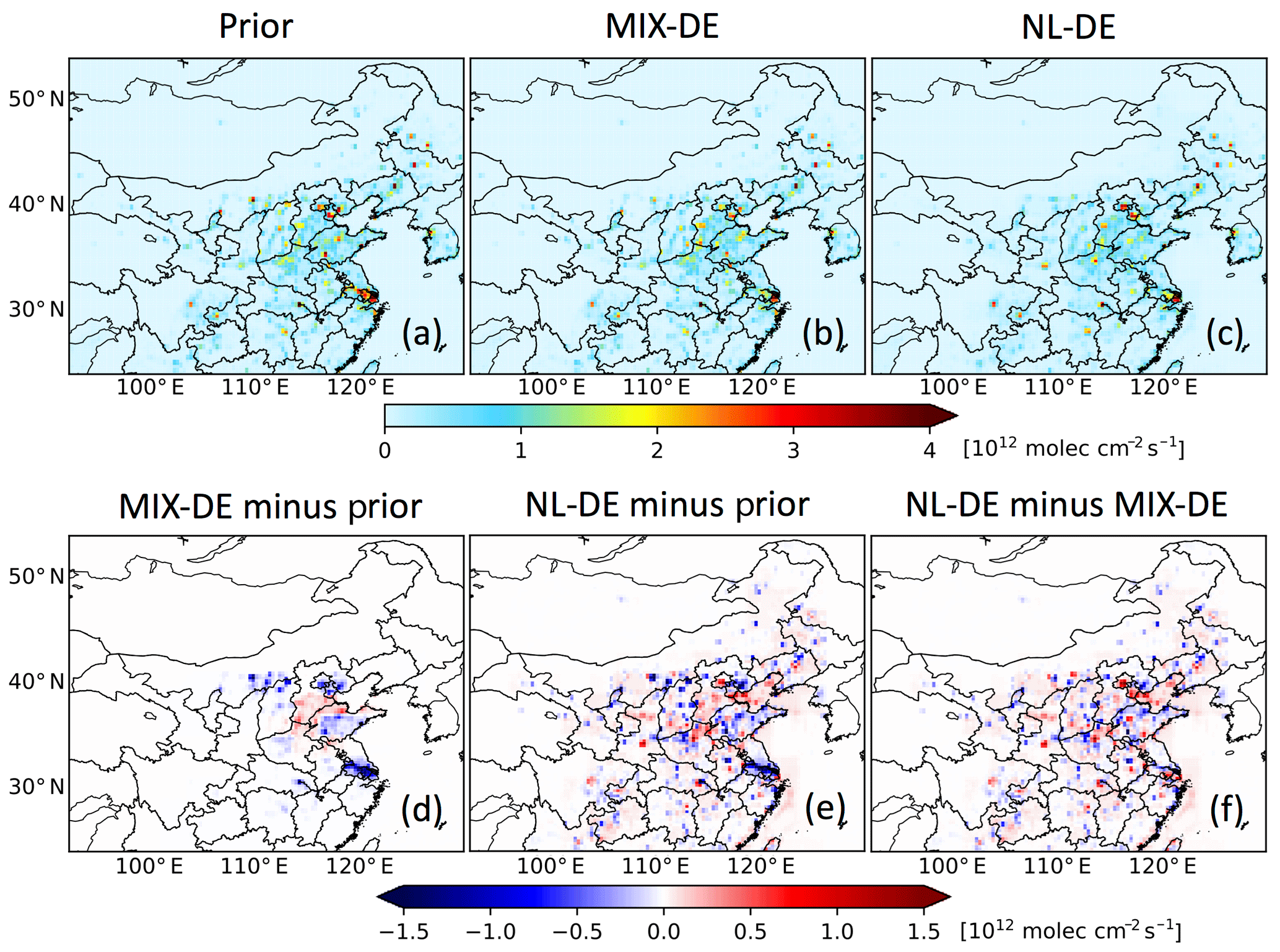
Figure 9 NO_x $\mathrm{0.25}{}^{\circ }\times \mathrm{0.3125}{}^{\circ }$ emissions of prior MIX 2010 (a), posterior MIX-DE (b), posterior NL-DE (c), the difference between posterior MIX-DE and prior MIX 2010 (d), the difference between posterior NL-DE and prior MIX 2010 (e), and the difference between posterior NL-DE and posterior MIX-DE (f).

Figure 10 Evaluations of fine-resolution GEOS-Chem surface NO₂ simulations with in situ observations for October 2013. Panels (a)–(c) show surface NO₂ concentrations of F-PRI, MIX-DE-POS, and NL-DE-POS, respectively, with in situ observations overlapped. Panels (d)–(f) show scatter plots of F-PRI, MIX-DE-POS, and NL-DE-POS simulations versus in situ observations, respectively. The linear correlation coefficient (R), normalized centered root mean squared error (NCRMSE), normalized mean squared error (NMSE), normalized mean bias (NMB), mean bias (MB), and number of observations (N) are shown over scatter plots.

MIX-DE-POS has improved values of R and NCRMSE compared to NL-DE-POS; here we discuss the possible reasons and propose future works to improve NL-DE. MIX is a mosaic bottom-up emission inventory, and it is actually the MEIC emission inventory for NO_x emissions over China (Li et al., 2017a). The MIX (or MEIC) NO_x emission inventory over China consists of emissions from four sectors including coal-fired power plant, industrial, transport, and residential sectors. Coal-fired power plant emissions in MEIC are derived through extensively using detailed information (including locations of individual units) of 7657 generation units in China (Liu et al., 2015); coal-fired power plant emissions can be accurately placed in grids according to source location information (Li et al., 2017a). Thus, if we can allocate posterior total anthropogenic NO_x emissions into the four sectors, we expect that it is better to use the MIX coal-fired power plant NO_x emission inventory rather than nighttime lights to downscale the posterior coal-fired power plant NO_x emissions. For the other sectors in MIX (or MEIC) over China, population density is used to allocate industrial and residential emissions to grids (Li et al., 2017a), and transport emissions are distributed according to road networks (Li et al., 2017a). Using population density to downscale industrial and residential NO_x could underestimate emissions over urban regions, compared with the approach using nighttime light which could better represent economic development levels (Geng et al., 2017). Whether it is better to use road networks or nighttime lights to downscale NO_x emissions from the transport sector requires future investigations. In this study, the posterior NO_x emission inventory to be downscaled is total anthropogenic NO_x emissions, which is not allocated into different source sectors. Thus, if we assume that the ratios of every sectoral emissions to total anthropogenic emissions do not change between prior and posterior emission inventories, MIX-DE has an advantage for the coal-fired power sector, while NL-DE could benefit the downscaling for the industrial and residential sectors. In future work, we could optimize sectoral emissions rather than total anthropogenic emissions, subsequently downscale posterior coal-fired power emissions through prior MIX coal-fired power emissions, and ultimately use VIIRS nighttime light data to downscale posterior industrial and residential emissions.

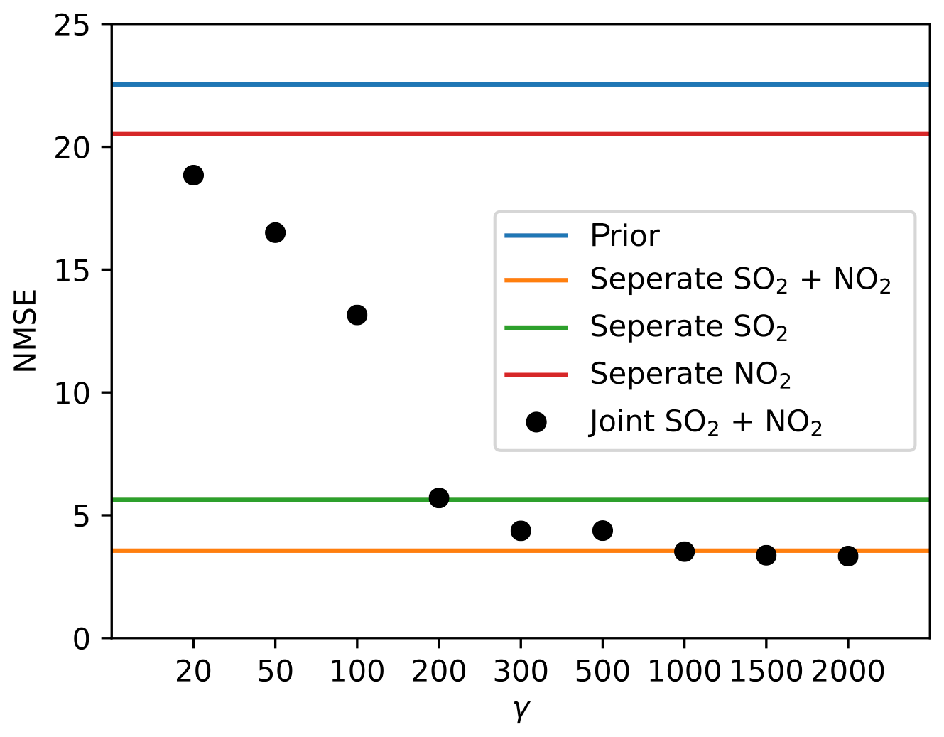
Figure 11 Sum of normalized mean squared error (NMSE) of surface SO₂ and NO₂. All surface SO₂ and NO₂ simulations come from MIX-DDC and NL-DC, respectively. Black dots are posterior simulations from Joint-F-POS. The blue line shows prior simulation results with SO₂ NMSE from MIX-DDC-PRI and NO₂ NMSE from NL-DC-PRI. The orange line shows simulation results with SO₂ NMSE from MIX-DDC-POS and NO₂ NMSE from NL-DC-POS. The green line is similar to the orange line, but the posterior SO₂ emission from separate assimilation and prior NO_x emission are used. The red line is similar to the orange line, but the posterior NO_x emission from separate assimilation and prior SO₂ emission are used.

Figure 12 Evaluation of GEOS-Chem surface SO₂ and NO₂ forecasts with in situ observations for November 2013. Panels (a) and (b) show scatter plots of AQF-PRI and AQF-MIX-DE-POS SO₂ at $\mathrm{0.25}{}^{\circ }\times \mathrm{0.3125}{}^{\circ }$ versus in situ province-capital-city observations, respectively. Panels (c) and (d) show scatter plots of AQF-PRI and AQF-MIX-DE-POS NO₂ at $\mathrm{0.25}{}^{\circ }\times \mathrm{0.3125}{}^{\circ }$ versus in situ observations, respectively. Panels (e) and (f) show scatter plots of AQF-NL-DC-PRI and AQF-NL-DC-POS NO₂ at $\mathrm{0.05}{}^{\circ }\times \mathrm{0.05}{}^{\circ }$ versus in situ observations, respectively. The linear correlation coefficient (R), normalized centered root mean squared error (NCRMSE), normalized mean squared error (NMSE), normalized mean bias (NMB), mean bias (MB), and number of observations (N) are shown over scatter plots.

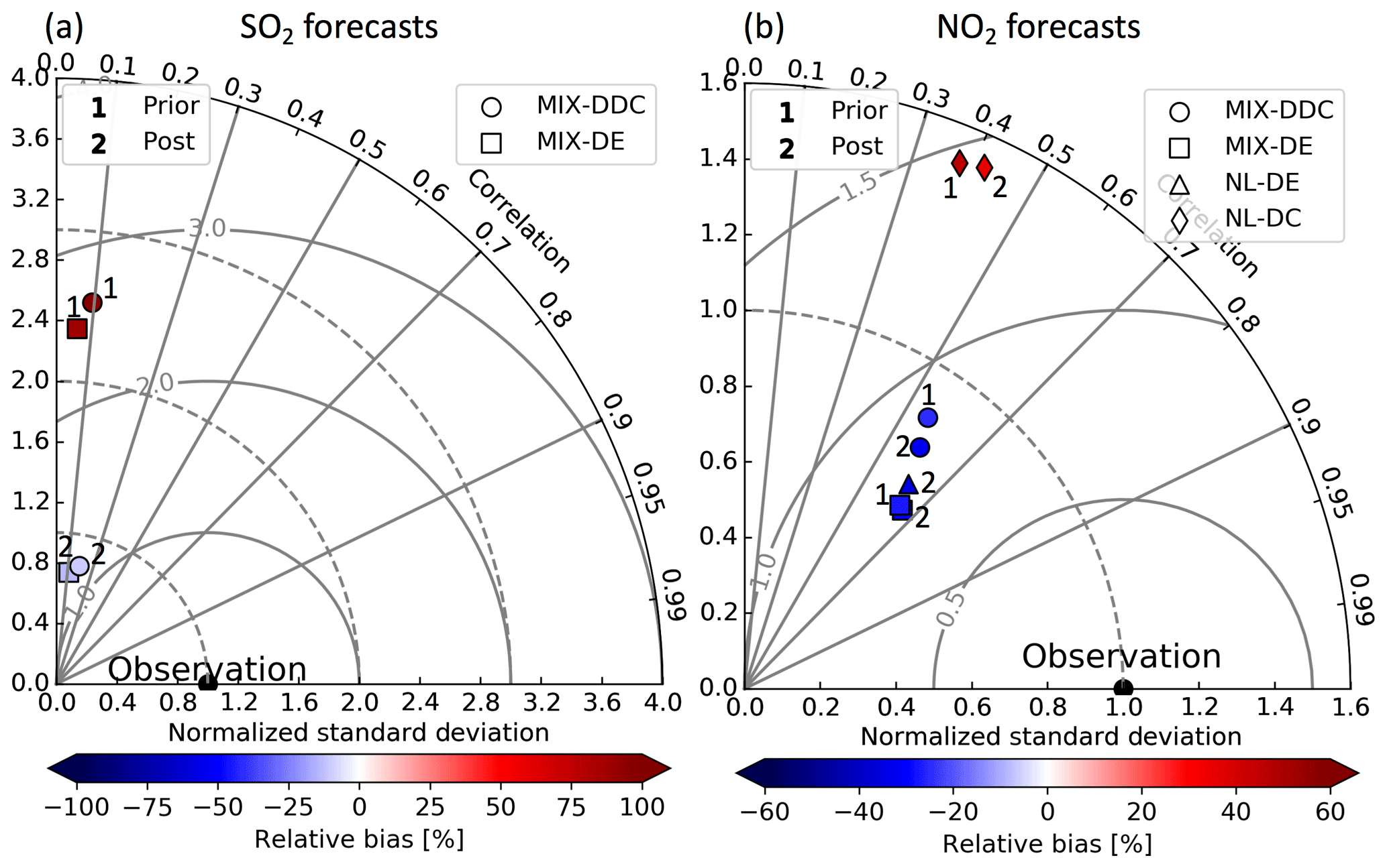
Figure 13 Taylor diagrams of evaluations of surface SO₂ (a) and NO₂ (b) forecasts with in situ observations. Circle 1 represents AQF-MIX-DDC-PRI, circle 2 AQF-MIX-DDC-POS, square 1 AQF-PRI, square 2 AQF-MIX-DE-POS, triangle 2 AQF-NL-DE-POS, diamond 1 AQF-NL-DC-PRI, and diamond 2 AQF-NL-DC-POS.

4.5 Impacts of joint assimilations on surface SO₂ and NO₂ simulations

To evaluate the posterior SO₂ and NO_x emissions of joint assimilations with various observation balance parameter (γ) values from Part 1, i.e., Wang et al. (2020), we focus on the sum of NMSE of surface SO₂ and NO₂ as shown in Fig. 11. The experiment using the prior MIX SO₂ and NO_x emissions has the largest sum of NMSE, which is followed by the simulation using the prior MIX SO₂ emissions and the posterior NO_x emissions from separate assimilation. The sum of NMSE using the posterior SO₂ and NO_x emissions of joint assimilations (JOINT-F-POS) with various observation balance parameter (γ) values (as γ increases, the NO₂ species is more emphasized in the cost function) is always smaller than that of the experiment using the prior MIX SO₂ emissions and the posterior NO_x emission from separate assimilation and decreases as γ increases. When γ is 1500 or 2000, the sum of NMSE using the posterior SO₂ and NO_x emissions of joint assimilations is smaller than that of the experiment using the prior MIX NO_x emission and the posterior SO₂ emission from separate assimilation, but it equals that of the experiment using the posterior SO₂ and NO_x emissions from separate assimilations. The value of γ mainly affects SO₂ NMSE (Fig. S4a) rather than NO₂ NMSE (Fig. S4b).

4.6 Application for forecasts

Figure 12 shows evaluations of surface SO₂ and NO₂ forecasts with in situ observations. AQF-PRI SO₂ concentrations are generally larger than in situ observations with MB of 45.07 µg m⁻³ and NMSE of 7.97 (Fig. 12a). The MB and NMSE reduces to −7.12 µg m⁻³ and 1.38 (Fig. 12b), respectively, in AQF-MIX-DE-POS. For surface NO₂, NCRMSE and R are 0.76 and 0.65 (Fig. 12c), respectively, in AQF-PRI and change to 0.75 and 0.66 (Fig. 12d), respectively, in AQF-MIX-DE-POS. The stronger negative NMB and larger NMSE for NO₂ in AQF-MIX-DE-POS than that in AQF-PRI are likely attributable to the CGS effect. The CGS effect is eliminated in both the AQF-NL-DC-PRI and AQF-NL-DC-POS, which show positive bias (Fig. 12e, f). In the $\mathrm{0.05}{}^{\circ }\times \mathrm{0.05}{}^{\circ }$ forecasts, NMSE decreases from 4.61 in AQF-NL-DC-PRI to 3.43 in AQF-NL-DC-POS, and R increases from 0.38 to 0.42.

In this study, we show the improvements of GEOS-Chem simulations or forecasts of surface SO₂ and NO₂ concentrations through posterior emissions constrained by integration of GEOS-Chem adjoint and OMPS observations. All the improvements of SO₂ and NO₂ forecasts are summarized in the Taylor diagrams (Fig. 13), which includes R, normalized standard deviation (the ratio of forecast standard deviation to in situ observations), NMB, and normalized centered root mean square error (NCRMSE). NCRMSE is shown as the distance between the forecast point and the expected (in situ observation) point. The improvements of forecasting surface SO₂ concentrations through MIX-DE and MIX-DDC are comparable (Fig. 13a). For NO₂ forecast, MIX-DE shows larger improvement than NL-DE and MIX-DDC (Fig. 13b). NL-DC is able to better decrease the coarse-grid smearing effect than MIX-DE but shows a larger normalized centered root mean square error. In the future, we plan to investigate if the posterior emissions can be applied to other models such as WRF-Chem and WRF-GC at a spatial resolution finer than $\mathrm{0.25}{}^{\circ }\times \mathrm{0.3125}{}^{\circ }$. In the case of the global model of chemistry, it is promising to use nighttime light to downscale NO₂ simulations so as to obtain a quick look of NO₂ air quality at very fine resolution.

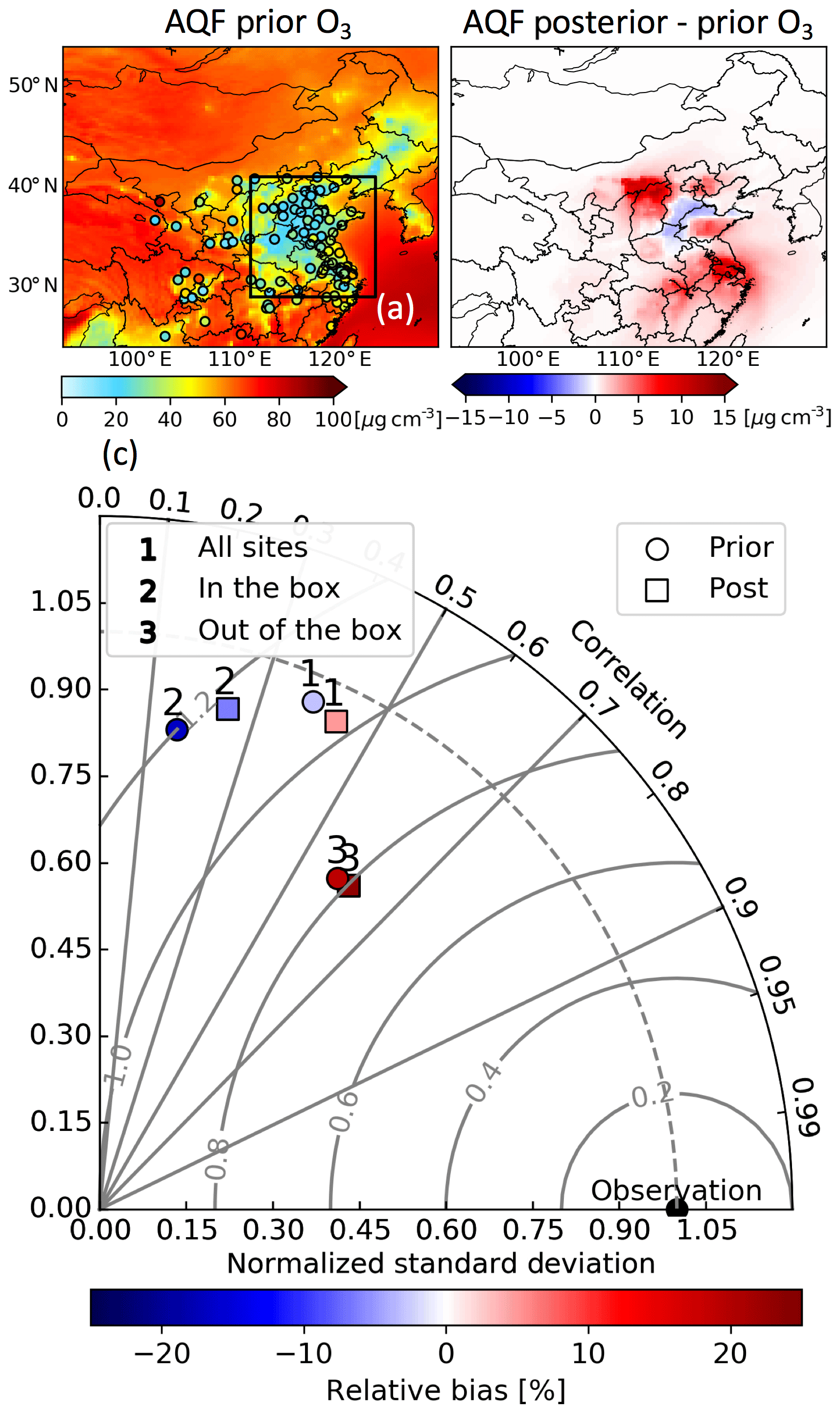
Figure 14 Evaluation of GEOS-Chem surface O₃ forecasts with in situ observations for November 2013. Panel (a) shows AQF-PRI O₃ forecasts with in situ observations overlapped. Panel (b) shows the difference between and AQF-MIX-DE-POS and AQF-PRI O₃ forecasts. Panel (c) shows the Taylor diagram of evaluations of surface O₃ forecasts in (a) and (b) with in situ observations. Circles and squares represent the AQF-PRI and AQF-MIX-DE-POS forecasts, respectively. Labels 1, 2, and 3 represent that all sites, only sites that are within the black box in (a), and only sites that are outside of the black box in (a) are used for evaluations.

In addition to the improvement of SO₂ and NO₂, AQF-MIX-DE-POS enhances AQF-PRI in the forecast of surface O₃ concentrations (Fig. 14). If all O₃ in situ observations in the research domain are used for evaluation, a spatial distribution improvement is shown with NCRMSE decreasing from 1.08 for AQF-PRI to 1.05 for AQF-MIX-DE-POS, but NMB changes from −3.1 % to 5.0 % (Fig. 14c). Indeed, whether bias becomes smaller or larger depends on the region. In the North China Plain and eastern China where NO_x emissions (or NO₂ surface concentrations) are large (the black box in Fig. 14a), forecasts of surface O₃ concentration are much lower than in other regions; and the NMB is −16.7 % for AQF-PRI and −6.3 % for AQF-MIX-DE-POS, with NCRMSE decreasing from 1.20 to 1.16 (Fig. 14c). In this relatively NO_x-rich region, the increase in O₃ concentration in AQF-MIX-DE-POS is caused by the decrease in NO₂ concentrations; the change in SO₂ concentrations has negligible impacts on O₃ concentrations (Fig. S5). This implies that if volatile organic compound (VOC) concentrations remain constant, emission control of NO_x emissions will exacerbate O₃ pollution. For the region that is outside of the black box, although NCRMSE decreases from 0.82 for AQF-PRI to 0.80 for AQF-MIX-DE-POS, NMB increases from 19.0 % to 23.3 % (Fig. 14c).

5 Discussion and conclusions

The posterior SO₂ and NO_x emissions at $\mathrm{2}{}^{\circ }\times \mathrm{2.5}{}^{\circ }$ resolution constrained by OMPS SO₂ and NO₂ retrievals through the GEOS-Chem adjoint model (Wang et al., 2020) are expected to improve simulations and forecasts of SO₂ and NO₂ pollution, but model simulation at such a coarse resolution fails to capture hot spots over cities due to the coarse-grid smearing or CGS effect, which prompts the study and development of downscaling techniques. Here, we introduce several downscaling approaches to obtaining surface SO₂ and NO₂ concentrations at finer resolution, which are further validated with in situ observations. All these methods are demonstrated through simulations of SO₂ and NO₂ for October 2013 and forecasts of SO₂, NO₂, and O₃ for November 2013 over China.

GEOS-Chem $\mathrm{2}{}^{\circ }\times \mathrm{2.5}{}^{\circ }$ simulations of surface SO₂ and NO₂ over China in October 2013 using the prior MIX 2010 emissions and the posterior emissions show negative bias due to the coarse-grid smearing (CGS) effect. The coarse-resolution simulations are downscaled to $\mathrm{0.25}{}^{\circ }\times \mathrm{0.3125}{}^{\circ }$ resolution according to the distributions of $\mathrm{0.25}{}^{\circ }\times \mathrm{0.3125}{}^{\circ }$ simulations based on the prior MIX 2010 emissions (MIX-DDC approach). When comparing with in situ surface observations, the MIX-DDC posterior SO₂ and NO₂ simulations show the normalized centered root mean squared error (NCRMSE) is 63.7 % and 30.2 %, respectively, lower than the MIX-DDC prior simulations. Compared with the $\mathrm{2}{}^{\circ }\times \mathrm{2.5}{}^{\circ }$ simulations, the downscaled $\mathrm{0.25}{}^{\circ }\times \mathrm{0.3125}{}^{\circ }$ simulations alleviate the CGS effect but do not avoid it completely. To further decrease the CGS effect for NO₂, we further downscale the surface NO₂ simulations from $\mathrm{2}{}^{\circ }\times \mathrm{2.5}{}^{\circ }$ to $\mathrm{0.05}{}^{\circ }\times \mathrm{0.05}{}^{\circ }$ according to VIIRS nighttime light observations, which are strongly related with TROPOMI NO₂ tropospheric VCDs (NL-DC approach). The NL-DC NO₂ posterior simulation is better than the NL-DC prior simulation when compared with in situ observations with NCRMSE decreasing from 1.34 to 1.10, and the MB decreases from 18.30 to 10.29 µg m⁻³. In terms of evaluating the downscaled SO₂ and NO₂ simulations simultaneously, using posterior SO₂ and NO_x emission inventories from joint assimilation is better than only using one (SO₂ or NO_x) emission inventory from separate assimilation, and it is similar to using posterior SO₂ and NO_x emission inventories from separate assimilation.

Instead of using prior fine-resolution simulations to downscale posterior coarse-resolution surface SO₂ and NO₂ concentrations, another approach is downscaling posterior emissions for $\mathrm{0.25}{}^{\circ }\times \mathrm{0.3125}{}^{\circ }$ simulations. We downscale the posterior $\mathrm{2}{}^{\circ }\times \mathrm{2.5}{}^{\circ }$ SO₂ emissions according to the distributions of fine-resolution prior MIX SO₂ emissions (MIX-DE). In the $\mathrm{0.25}{}^{\circ }\times \mathrm{0.3125}{}^{\circ }$ simulations, posterior surface SO₂ is in better agreement with in situ observations than the prior. Not only are the fine-resolution prior MIX NO_x emissions used to downscale posterior $\mathrm{2}{}^{\circ }\times \mathrm{2.5}{}^{\circ }$ NO_x emissions, we also use VIIRS nighttime light observations as proxies to downscale posterior $\mathrm{2}{}^{\circ }\times \mathrm{2.5}{}^{\circ }$ NO_x emissions (NL-DE approach). All these emissions are used to simulate surface NO₂ concentrations, which are validated with in situ observations. The simulations using MIX-DE and NL-DE posterior NO_x emissions show smaller root mean square error and larger linear correlation than the prior simulation. The NO₂ simulation using MIX-DE emissions shows better results than that using NL-DE emissions, which may be owing to all NO_x emissions being treated as area sources in the NL-DE approach while the MIX-DE approach has point source information, if we assume that sectoral ratios do not change between prior and posterior emissions. We also notice that using the prior fine-resolution simulations to downscale the posterior coarse-resolution surface SO₂ and NO₂ concentrations is slightly better than simulations using the downscaled posterior emissions.

To study the feasibility of improving surface SO₂, NO₂, and O₃ predictions, posterior emission inventories of the current month are scaled to the next month according to the monthly variations of the prior MIX emission inventory and are subsequently applied to forecasts of the next month. Here we integrate MIX-DE posterior SO₂ and NO_x emission inventories for October 2013 and the monthly scale factors derived from the prior MIX emission inventory to obtain posterior SO₂ and NO_x emission inventories for November 2013. These are further used to forecast surface SO₂, NO₂, and O₃ concentrations at $\mathrm{0.25}{}^{\circ }\times \mathrm{0.3125}{}^{\circ }$ for November 2013, and the results are better than using prior emissions when evaluated with in situ observations, although the CGS effect is not completely avoided at this spatial resolution for SO₂ and NO₂. The forecasts of surface NO₂ concentrations at $\mathrm{0.05}{}^{\circ }\times \mathrm{0.05}{}^{\circ }$ resolutions through NL-DC can eliminate the CGS effect, and the posterior forecast is also in better agreement with in situ observations than the prior forecast.