the Creative Commons Attribution 4.0 License.
the Creative Commons Attribution 4.0 License.
 | 03 Jan 2020
Retrieving the global distribution of the threshold of wind erosion from satellite data and implementing it into the Geophysical Fluid Dynamics Laboratory land–atmosphere model (GFDL AM4.0/LM4.0)
Paul Ginoux
N. Christina Hsu
John Kimball
Beatrice Marticorena
Sergey Malyshev
Vaishali Naik
Norman T. O'Neill
Carlos Pérez García-Pando
Juliette Paireau
Joseph M. Prospero
Elena Shevliakova
Ming Zhao
Dust emission is initiated when surface wind velocities exceed the threshold of wind erosion. Many dust models used constant threshold values globally. Here we use satellite products to characterize the frequency of dust events and land surface properties. By matching this frequency derived from Moderate Resolution Imaging Spectroradiometer (MODIS) Deep Blue aerosol products with surface winds, we are able to retrieve a climatological monthly global distribution of the wind erosion threshold (Vthreshold) over dry and sparsely vegetated surfaces. This monthly two-dimensional threshold velocity is then implemented into the Geophysical Fluid Dynamics Laboratory coupled land–atmosphere model (AM4.0/LM4.0). It is found that the climatology of dust optical depth (DOD) and total aerosol optical depth, surface PM10 dust concentrations, and the seasonal cycle of DOD are better captured over the “dust belt” (i.e., northern Africa and the Middle East) by simulations with the new wind erosion threshold than those using the default globally constant threshold. The most significant improvement is the frequency distribution of dust events, which is generally ignored in model evaluation. By using monthly rather than annual mean Vthreshold, all comparisons with observations are further improved. The monthly global threshold of wind erosion can be retrieved under different spatial resolutions to match the resolution of dust models and thus can help improve the simulations of dust climatology and seasonal cycles as well as dust forecasting.
- Article
(17167 KB) - Full-text XML
-
Supplement
(2181 KB) - BibTeX
- EndNote


Mineral dust is one of the most abundant aerosols by mass and plays an important role in the climate system. Dust particles absorb and scatter solar and terrestrial radiation, thus modifying the local energy budget and consequently atmospheric circulation patterns. Studies have shown that the radiative effect of dust can affect a wide range of environmental processes. Dust is shown to modulate western African (e.g., Miller and Tegen, 1998; Miller et al., 2004; Mahowald et al., 2010; Strong et al., 2015) and Indian (e.g., Jin et al., 2014, 2015, 2016; Vinoj et al., 2014; Solmon et al., 2015; Kim et al., 2016; Sharma and Miller, 2017) monsoonal precipitation. During severe droughts in North America, there is a positive feedback between dust and the hydrological cycle (Cook et al., 2008, 2009, 2013). African dust is also found to affect Atlantic tropical cyclone activity (e.g., Dunion and Velden, 2004; Wong and Dessler, 2005; Evan et al., 2006; Strong et al., 2018). When deposited on snow and ice, dust reduces the surface reflectivity, enhancing net radiation and accelerating snow and ice melting and consequently affecting runoff (e.g., Painter et al., 2010, 2018; Dumont et al., 2014). Dust can serve as ice nuclei and affect the formation, lifetime, and characteristic of clouds (e.g., Levin et al., 1996; Rosenfield et al., 1997; Wurzler et al., 2000; Nakajima et al., 2001; Bangert et al., 2012), perturbing the hydrological cycle. Iron- and phosphorus-enriched dust is also an important nutrient for the marine and terrestrial ecosystems and thus interacts with the ocean and land biogeochemical cycles (e.g., Fung et al., 2000; Jickells et al., 2005; Shao et al., 2011; Bristow et al., 2010; Yu et al., 2015).
Given the importance of mineral dust, many climate models incorporate dust emission schemes to simulate the life cycle of dust aerosols (e.g., Donner et al., 2011; Collins et al., 2011; Watanabe et al., 2011; Bentsen et al., 2013). Mineral dust particles are lifted from dry and bare soils into the atmosphere by saltation and sandblasting. This process is initiated when surface winds reach a threshold velocity of wind erosion. The value of this wind erosion threshold depends on soil and surface characteristics, including soil moisture, soil texture, and particle size, and the presence of pebbles, rocks, and vegetation residue (e.g., Gillette et al., 1980; Gillette and Passi, 1988; Raupach et al., 1993; Fécan et al., 1999; Zender et al., 2003; Mahowald et al., 2005), and this thus varies spatially and temporally (Helgren and Prospero, 1987). Due to a lack of in situ data at a global scale and uncertainties on these dependencies, most dust and climate models prescribe a spatially and temporally constant threshold of wind erosion for surface 10 m wind (e.g., around 6 to 6.5 m s−1) over dry surfaces for simplicity (e.g., Tegen and Fung, 1994; Takemura et al., 2000; Uno et al., 2001; Donner et al., 2011). For instance, in the Geophysical Fluid Dynamics Laboratory coupled land–atmosphere model AM4.0/LM4.0 (Zhao et al., 2018a, b), a constant threshold of 6 m s−1 is used. On the other hand, some models, such as the Hamburg version of the European Centre for Medium-Range Weather Forecasts (ECMWF) model Hamburg Aerosol Module (ECHAM-HAM), Hadley Centre Global Environmental Model, version 2, Earth System (HadGEM2-ES), and ICOsahedral Nonhydrostatic – Aerosol and Reactive Trace gases (ICON-ART), parameterize the constant dry threshold friction velocity (usually a function of soil particle size, soil, and air density) or threshold wind velocity with dependencies on soil moisture, surface roughness length, and vegetation coverage (e.g., Takemura et al., 2000; Ginoux et al., 2001; Zender et al., 2003; Cheng et al., 2008; Jones et al., 2011; Rieger et al., 2017).
The threshold of wind erosion may be approximately inferred using observations. For instance, Chomette et al. (1999) used the Infrared Difference Dust Index (IDDI) and 10 m winds reanalysis from the ECMWF between 1990 and 1992 to calculate the threshold of wind erosion over seven sites over the Sahel and Sahara. The IDDI was used to determine whether there was a dust event for subsequently calculating an emission index defined as the number of dust events to the total number of potential events. The distribution of surface wind speed was matched with the emission index, and the threshold of wind erosion was determined when the emission index was around 0.9. The resulting average threshold of wind erosion ranged from 6.63 m s−1 at a Sahelian site to about 9.08 m s−1 at a Niger site, consistent with the model results by Marticorena et al. (1997).
Later, Kurosaki and Mikami (2007) used World Meteorological Organization (WMO) station data from March 1998 to June 2005 to examine the threshold wind speed in eastern Asia. Using the distribution of surface wind speed and associated weather conditions (i.e., with or without dust emission events), they approximated a dust emission frequency by dividing the number of dust events by the total number of observations for each wind bin, and then they determined threshold wind speeds at the 5 % and 50 % levels, corresponding to the most favorable and normal land surface conditions for dust emission, respectively. They found that the derived threshold wind speed varied in space and time, with a larger seasonal cycle in grassland regions, such as northern Mongolia, and smaller seasonal variations in desert regions, such as the Taklimakan and Gobi deserts and the Loess Plateau. Cowie et al. (2014) applied a similar method over northern Africa, using wind data observed between 1984 and 2012, and they focused on threshold winds at the 25 %, 50 %, and 75 % levels.
Draxler et al. (2010) derived the distribution of the threshold of friction velocity over the US by matching the frequency of occurrence (FoO) of Moderate Resolution Imaging Spectroradiometer (MODIS) Deep Blue (Hsu et al., 2004) aerosol optical depth (AOD) above 0.75 with the FoO of friction velocities extracted from the North American Mesoscale (NAM) forecast model at each grid point. This new threshold and a soil characteristics factor was then incorporated into the Hybrid Single-Particle Lagrangian Integrated Trajectory (HYSPLIT) model (Draxier and Hess, 1998) to forecast dust surface concentrations. It was found that major observed dust plume events in June and July 2007 were successfully captured by the model. Later, Ginoux and Deroubaix (2017) used FoO derived from the MODIS Deep Blue dust optical depth (DOD) record to retrieve the wind erosion threshold of surface 10 m winds over eastern Asia.
For individual dust events, the threshold of friction velocity can also be determined by fitting a 2nd-order Taylor series to dust saltation flux measurements (Barchyn and Hugenholtz, 2011; Kok et al., 2014b).
Nonetheless, a global distribution of the threshold of wind erosion with observational constraints that may be implemented in climate models is still lacking. In this study, we propose a method to retrieve the monthly global threshold of wind erosion (hereafter, Vthreshold) for dry and sparsely vegetated surface (i.e., under favorable conditions for dust emission) using high-resolution satellite products and reanalysis datasets. This two-dimensional threshold of surface 10 m winds is then implemented into the Geophysical Fluid Dynamics Laboratory (GFDL) coupled land–atmosphere model, AM4.0/LM4.0 (Zhao et al., 2018a, b). The benefits of using this spatially and temporally varying threshold in simulating present-day climatology and seasonal cycles of dust are analyzed by comparing the model results with observations.
The data and method used to retrieve the threshold of wind erosion are detailed in Sect. 2. The distribution of the derived Vthreshold and its implication in the climate model is presented in Sect. 3. Section 4 discusses the uncertainties associated with this method, and major conclusions are summarized in Sect. 5.
In this section we first introduce the satellite products, observational data, and reanalyses used to retrieve the threshold of wind erosion and validate model output (Sect. 2.1). The processes to retrieve the threshold of wind erosion are detailed in Sect. 2.2. The uncertainties of Vthreshold associated with the retrieval criteria and selection of surface wind datasets are discussed in Sect. 2.3. Section 2.4 introduces the GFDL AM4.0/LM4.0 model, its dust emission scheme, and simulation designs.
2.1 Data
2.1.1 Satellite products
-
MODIS Aqua and Terra dust optical depth. DOD is column-integrated extinction by mineral particles. Here daily DOD is retrieved from MODIS Deep Blue aerosol products (collection 6, level 2; Hsu et al., 2013; Sayer et al., 2013): aerosol optical depth (AOD), single-scattering albedo (ω), and the Ångström exponent (α). All the daily variables are first interpolated to a 0.1 × 0.1∘ grid using the algorithm described by Ginoux et al. (2010). We require the single-scattering albedo at 470 nm to be less than 0.99 for dust due to its absorption of solar radiation. This separates dust from scattering aerosols, such as sea salt. Then a continuous function relating the Ångström exponent, which is highly sensitive to particle size (Eck et al., 1999), to fine-mode AOD established by Anderson et al. (2005; their Eq. 5) is used to separate dust from fine particles. In short, DOD is retrieved using the following equation:
Details about the retrieval process and estimated errors are summarized by Pu and Ginoux (2018b). High-resolution MODIS DOD products (0.1 × 0.1∘) have been used to identify and characterize dust sources (Ginoux et al., 2012; Baddock et al., 2016) and examine the variations in dustiness in different regions (e.g., Pu and Ginoux, 2016, 2017, 2018b).
Following the recommendation from Baddock et al. (2016), who found the dust sources are better detected using DOD with a low-quality flag (i.e., quality assurance flag, QA, equals 1, following the category of retrieval quality flags in MODIS Deep Blue products; Hsu et al., 2013) than with a high-quality flag (i.e., QA = 3); as retrieved aerosol products were poorly flagged over dust source regions, we also use DOD with the flag of QA = 1. Both daily DOD retrieved from Aqua and Terra platforms are used by averaging the two when both products are available or using either one when only one product is available. Since Terra passes the Equator from north to south around 10:30 local time (LT) and Aqua passes the Equator from south to north around 13:30 LT, an average of the two combines the information from both morning and afternoon hours. This process also largely reduces missing data (Pu and Ginoux, 2018b). This combined daily DOD, hereafter MODIS DOD, is available from January 2003 to December 2015 at a resolution of 0.1 × 0.1∘ grid. Note that due to the temporal coverage of MODIS products, the diurnal variations in dust (e.g., O'rgill and Sehmel, 1976; Mbourou et al., 1997; Knippertz, 2008; Schepanski et al., 2009) are not included in current study.
-
Soil moisture. Soil moisture is an important factor that affects dust emission (Fécan et al., 1999). Daily surface volumetric soil moisture (VSM) retrievals derived from similar calibrated microwave (10.7 GHz) brightness temperature observations from the Advanced Microwave Scanning Radiometer for the Earth Observing System (AMSR-E) onboard the NASA Aqua satellite (from June 2002 to October 2011) and the Advanced Microwave Scanning Radiometer 2 (AMSR2) sensor onboard the JAXA GCOM-W1 satellite (from July 2012 to June 2017) from the University of Montana (Du et al., 2017a, b) was used to retrieve the wind erosion threshold. Both AMSR-E and AMSR2 sensors provide global measurements of polarized microwave emissions at six channels, with ascending and descending orbits crossing the Equator at around 13:30 and 01:30 LT respectively. The VSM retrievals are derived from an iterative retrieval algorithm that exploits the variable sensitivity of different microwave frequencies and polarizations and minimizes the potential influence of atmosphere, vegetation, and surface water cover on the soil signal. The VSM record represents surface (top ∼ 2 cm) soil conditions and shows favorable global accuracy and consistent performance (Du et al., 2017b), particularly over areas with low-to-moderate vegetation cover that are also more susceptible to wind erosion, although cautions are needed when examining long-term trends due to the small biases between AMSR-E and AMSR2. The horizontal resolution of the product is about 25 km×25 km, and the daily product from January 2003 to December 2015 is used. The ascending and descending obit VSM retrievals are averaged to get the mean VSM for each day.
-
Snow cover. Snow cover may affect dust emission in the mid-latitudes during spring, for instance, over northern China (Ginoux and Deroubaix, 2017). The interannual variation of snow cover is also found to affect dust emission in regions such as Mongolia (Kurosaki and Mikami, 2004). Here monthly snow cover data from MODIS/Terra level 3 data (Hall and Riggs, 2015) with a resolution of 0.05 × 0.05∘ from 2003 to 2015 are used. The high spatial resolution of the product is very suitable for this study.
-
Leaf area index (LAI). Vegetation protects soil from the effects of wind and thus modulates dust emission (e.g., Marticorena and Bergametti, 1995; Zender et al., 2003). While dense vegetation coverage can increase surface roughness and reduce near-surface wind speed, the roots of vegetation can increase soil cohesion and further reduce wind erosion. LAI describes the coverage of vegetation with a unit of m2 m−2, i.e., leaf area per ground area. Here monthly LAI retrieved by Boston University from MODIS onboard Aqua (Yan et al., 2016a, b; Ranga Myneni and Taejin Park, Boston University, personal communication, 2016) with a resolution of 0.1 × 0.1∘ from 2003 to 2015 is used. The root mean square error of the product is 0.66, with some overestimation of LAI in sparsely vegetated regions (Yan et al. 2016b; Garrigues et al., 2008).
2.1.2 Reanalysis
Surface wind speed is a critical factor that affects wind erosion. Here 6-hourly 10 m wind speed from the NCEP/NCAR (National Centers for Environmental Prediction/National Center for Atmospheric Research) reanalysis (Kalnay et al., 1996, hereafter NCEP1) on a T62 Gaussian grid (i.e., 192 longitude grids equally spaced and 94 latitude grids unequally spaced) is used. The NCEP1 is a global reanalysis with relatively long temporal coverage, from 1948 to the present. We chose to use the NCEP1 reanalysis mainly because surface winds in the GFDL AM4.0 model are nudged toward the NCEP1, and we preferred to use the reanalysis surface wind that is closest to the model climatology.
ERA-Interim (ECMWF Reanalysis Interim; Dee et al., 2011) is a global reanalysis produced from ECMWF. It provides high spatial resolution (about 0.75∘ or 80 km) 6-hourly, daily, and monthly reanalysis from 1979 to present day. Soil temperature from the ERA-Interim is used to determine the regions where wind erosion may be prohibited by the frozen surface. Monthly temperature of the first soil layer (0 to 0.07 m) from 2003 to 2015 is used.
In order to quantify the uncertainties of the retrieved threshold wind erosion in association with the selection of reanalysis products, surface 10 m winds from 6-hourly ERA-Interim and hourly ERA5 (Hersbach and Dee, 2016) are both examined. The ERA5 is the latest reanalysis product from the ECMWF, with a horizontal resolution of about 31 km and hourly temporal resolution.
2.1.3 Station data
Multiple ground-based datasets are used to validate AM4.0/LM4.0 simulated aerosol and dust optical depth and surface dust concentrations.
-
AERONET. The AErosol RObotic NETwork (AERONET; Holben et al., 1998) provides quality-assured cloud-screened (level 2) aerosol measurements from sun photometer records. In this paper we used the data products of the version 3.0 AERONET processing routine. To examine model-simulated DOD, we used coarse-mode AOD (COD; i.e., radius > 0.6 µm) at 500 nm processed by the Spectral Deconvolution Algorithm (O'Neill et al., 2003; hereafter SDA). SDA COD monthly data are first screened to remove those months with less than 5 d of records. To get the annual means, years with less than 5 months of records were removed. Only stations with records of at least 3 years during the period were used to calculate the 2003–2015 climatology (the same time period when MODIS DOD is available). Overall, records from 313 stations were obtained.
AERONET monthly aerosol optical thickness (AOT) data around 550 nm (e.g., 500, 551, 531, 440, 675, 490, 870 nm, etc.) and the Ångström exponents across the dual wavelength of 440–675, 440–870, and 500–870 nm are used to calculate AOD at 550 nm (τ550). If AOT for 551, 555, 531 or 532 nm exist, then these values are directly used as AOD 550 nm. Otherwise, the AOT at wavelength λA (less than 550 nm; i.e., τA), AOT at wavelength λB (larger than 550 nm; i.e., τB), and Ångström exponent between wavelengths λA and λB (α) are used to derive AOD 550 nm using the following equations:
In a manner similar to the process of screening SDA COD data, monthly AOD 550 nm data with less than 3 d of records in a given month are removed. When calculating the annual means we excluded years having less than 5 months of records. Finally, to calculate the climatology of 2003–2015, only stations with at least 3 years of records during this period are used, totaling 351.
We also developed a method to derive DOD at 550 nm from AOD at 550 nm based on the relationship between the Ångström exponent and fine-mode AOD established by Anderson et al. (2005; their Eq. 5). This adds a few more sites over the Sahel than the SDA COD stations. DOD is calculated by subtracting fine-mode AOD from total AOD. Due to the large uncertainties of single-scattering albedo in AERONET records over regions where AOD is lower than 0.4 (e.g., Dubovik and King, 2000; Holben et al., 2006; Andrews et al., 2017), we did not use single-scattering albedo to screen AOD to further separate dust from scattering aerosols. Therefore, the derived AERONET DOD over coastal stations may be contaminated by sea salt.
-
RSMAS surface dust concentration. The Rosenstiel School of Marine and Atmospheric Science (hereafter the RSMAS dataset) at the University of Miami collected mass concentrations of dust, sea salt, and sulfate over stations globally, with most of the stations on islands (Savoie and Prospero, 1989). The dataset has been widely used for model evaluation (e.g., Ginoux et al., 2001; Huneeus et al., 2011).
Only stations with records longer than 4 years were used, and of those stations only those years with at least 8 months of data are used for calculating climatological annual means. So, in total 16 stations are used. Station names, locations, and record lengths are listed in Table S1 of the Supplement. We compare the climatology of annual mean surface dust concentration with model output during 2000–2015. Note that since most station records end earlier than 1998, the dataset largely represents the climatology during the 1980s and 1990s. Thus the discrepancies between model output and the RSMAS data include both model biases and the difference in surface dust concentration from the 1980s to the 2000s.
-
IMPROVE surface fine dust concentration. The Interagency Monitoring of Protected Visual Environments (IMPROVE) network has collected near-surface particulate matter 2.5 (PM2.5) samples in the US since 1988 (Malm et al., 1994; Hand et al., 2011). IMPROVE stations are located in national parks and wilderness areas, and PM2.5 sampling is performed twice weekly (Wednesday and Saturday; Malm et al., 1994) prior to 2000 and every third day afterwards. Fine dust (with an aerodynamic diameter less than 2.5 µm) concentration is calculated using the concentrations of aluminum (Al), silicon (Si), calcium (Ca), iron (Fe), and titanium (Ti) by assuming oxide norms associated with predominant soil species (Malm et al., 1994; their Eq. 5). This dataset has been widely used to study variations in surface fine dust in the US (e.g., Hand et al., 2016, 2017, Tong et al., 2017; Pu and Ginoux, 2018a). Here only monthly data with at least 50 % of the daily data available in a month (i.e., at least 5 records) are used. Since station coverage over the central US increases after 2002 (e.g., Pu and Ginoux, 2018a), monthly station data from 2002 to 2015 are used and interpolated to a 0.5 × 0.5∘ grid using inverse distance weighting interpolation. The gridded data are used to evaluate modeled surface fine dust concentrations.
-
LISA PM10 surface concentration. Surface PM10 concentrations from stations from the Sahelian Dust Transect, which was deployed in 2006 under the framework of the African Monsoon Multidisciplinary Analysis International Program (Marticorena et al., 2010), were used to examine the surface dust concentration over the Sahelian region. The data are maintained by the Laboratoire Interuniversitaire des Systèmes Atmosphériques (LISA) in the framework of the International Network to study Deposition and Atmospheric composition in Africa (INDAAF; Service National d'Observation de l'Institut National des Sciences de l'Univers, France). Three stations are located within the pathway of Saharan and Sahelian dust plumes moving towards the Atlantic Ocean. Here hourly PM10 concentrations from the stations in Banizoumbou (Niger, 13.54∘ N, 2.66∘ E), Cinzana (Mali, 13.28∘ N, 5.93∘ W), and M'Bour (Senegal, 14.39∘ N, 16.96∘ W) from 2006 to 2014 are used. The hourly station data are averaged to obtain daily and monthly mean records to compare with model output.
2.1.4 Other data
Soil depth from the Food and Agriculture Organization of the United Nations (FAO/IIASA/ISRIC/ISS-CAS/JRC, 2009) on a 0.08 × 0.08∘ resolution is used to examine whether the soil depth is too shallow (i.e., less than 15 cm) for wind erosion.
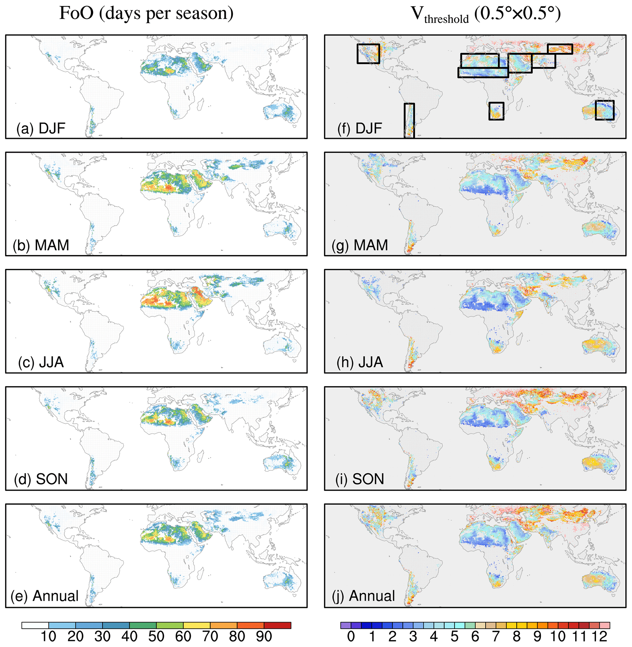
Figure 1(a–e) Frequencies of occurrence (FoO; unit: days per season) in each season and the annual mean. (f–j) Threshold of wind erosion (Vthreshold; unit: m s−1) derived from satellite products and reanalyses for each season and the annual mean using DODthresh=0.2 (or 0.02). Black boxes in (f) denote nine dust source regions as listed in Table 1.
2.2 Retrieving the threshold of wind erosion
The monthly climatological threshold of wind erosion is retrieved by matching the frequency distribution of the MODIS DOD at a certain level, namely, DODthresh, with the frequency distribution of surface 10 m winds from the NCEP1 reanalysis over the period from 2003 to 2015. The process can be summarized by the following steps:
-
Step 1. Since dust is emitted from the dry and sparsely vegetated surface, the daily DOD data are first masked out to remove the influences of non-erodible factors and unfavorable environmental conditions that are known to prevent dust emission using criteria as follows: daily VSM less than 0.1 cm3 cm−3; monthly LAI less than 0.3; monthly snow cover less than 0.2 % (since the snow cover percentage is rounded up to an integer in the MODIS product, this criterion actually requires no snow cover); monthly top-layer soil temperature higher than 273.15 K, i.e., over unfrozen surface; and soil depth thicker than 15 cm. These criteria approximate the most favorable land surface conditions for wind erosion.
Similar criteria have been used in previous studies to detect or confine dust source regions. For instance, Kim et al. (2013) used the normalized difference vegetation index (NDVI) for less than 0.15, soil depth greater than 10 cm, surface temperature greater than 260 K, and without snow cover to mask topography-based dust source function. LAI less than 0.3 has been used as a threshold for dust emission in the Community Land Model (Mahowald et al., 2010; Kok et al., 2014a), while gravimetric soil moisture ranging from 1.01 % to 11.2 % depending on soil clay content is recommended to constrain dust emission (Fécan et al., 1999). The uncertainties associated with small variations in the retrieval criteria are further quantified and discussed in Sect. 2.3.
-
Step 2. Masked daily DOD from Step 1 is then interpolated to a 0.5 × 0.5∘ grid using bilinear interpolation. This is close to the horizontal resolution of the GFDL AM4.0/LM4.0 model used in this study. Then the cumulative frequency distribution of daily DOD from 2003 to 2015 is derived at each grid point for each month.
-
Step 3. Daily maximum surface wind speed is first derived from 6-hourly NCEP1 surface winds and then interpolated to a 0.5 × 0.5∘ grid. Following Ginoux and Deroubaix (2017), we use maximum daily wind speed instead of daily mean wind speed, largely because dust emission only occurs when wind speed is strong enough, and the emission magnitude is roughly proportional to the third power of surface wind speed in empirical estimations. The cumulative frequency distribution of daily maximum surface wind from 2003 to 2015 is then calculated at each grid point for each month.
-
Step 4. A minimum value of DOD (i.e., DODthresh) is used to separate dust events from background dust. The cumulative frequency (as a percentage) of dust events passing this threshold is compared to the cumulative frequency of surface winds. The minimum surface winds with the same frequency correspond to the threshold of wind erosion, Vthreshold (see a schematic diagram in Fig. S1 in the Supplement). This operation is performed for all grid points for each month. Ginoux et al. (2012) used DODthresh=0.2 to separate dust events from background dust and quantify the FoO of local dust events. Similarly, DODthresh=0.2 is used here in major dusty regions (northern Africa, the Middle East, India, northern China), while for less dusty regions, such as the US, South America, South Africa, and Australia, DODthresh=0.02 is used. The reason to use a lower DODthresh for less dusty regions is because (i) the overall dust emission in these regions are at least 10 times smaller than major dusty regions, such as northern Africa (e.g., Huneeus et al., 2011) and (ii) the frequency distribution of DOD in these regions also peaks at a much lower DOD band (see discussion in Sect. 3.3). We also tested the DODthresh=0.5 for dusty regions and DODthresh=0.05 for less dusty regions, and results are discussed in Sects. 2.3 and 3.1.
Figure 1a–e show the seasonal and annual mean FoO (days when DOD is greater than DODthresh) using DODthresh=0.2 or 0.02. The shaded area covers major dust sources, and the pattern is very similar to that obtained by Ginoux et al. (2012; their Fig. 5), although there are some differences, largely due to the masked DOD (i.e., from Step 1) used in this study and a lower threshold in less dusty regions. The higher FoO in northern Africa during summer in comparison with other seasons is consistent with the summer peak of the frequency of the dust source activation derived from the Meteosat Second Generation (MSG) images (Schepanski et al., 2007; their Fig. 1). The relatively high value of FoO over the northern Sahel to southern Sahara is also consistent with dust emission frequency derived from the Meteosat Second Generation Spinning Enhanced Visible and Infrared Imager (Evan et al., 2015; their Fig. 1).
Note that the selections of masking criteria in Step 1 and DODthresh in Step 4 are empirical and can add uncertainties to this method. Also, we approximate dust emission using the cumulative frequency of DOD, which may overestimate dust emission in regions where the contribution of transported dust is significant, and thus we may underestimate the Vthreshold in those regions. These uncertainties are further discussed in the following section.
Table 1Major dust source regions shown in Fig. 1. Note that region names such as India and northern China are not exactly the same as their geographical definitions, as these regions also cover some areas from nearby countries.
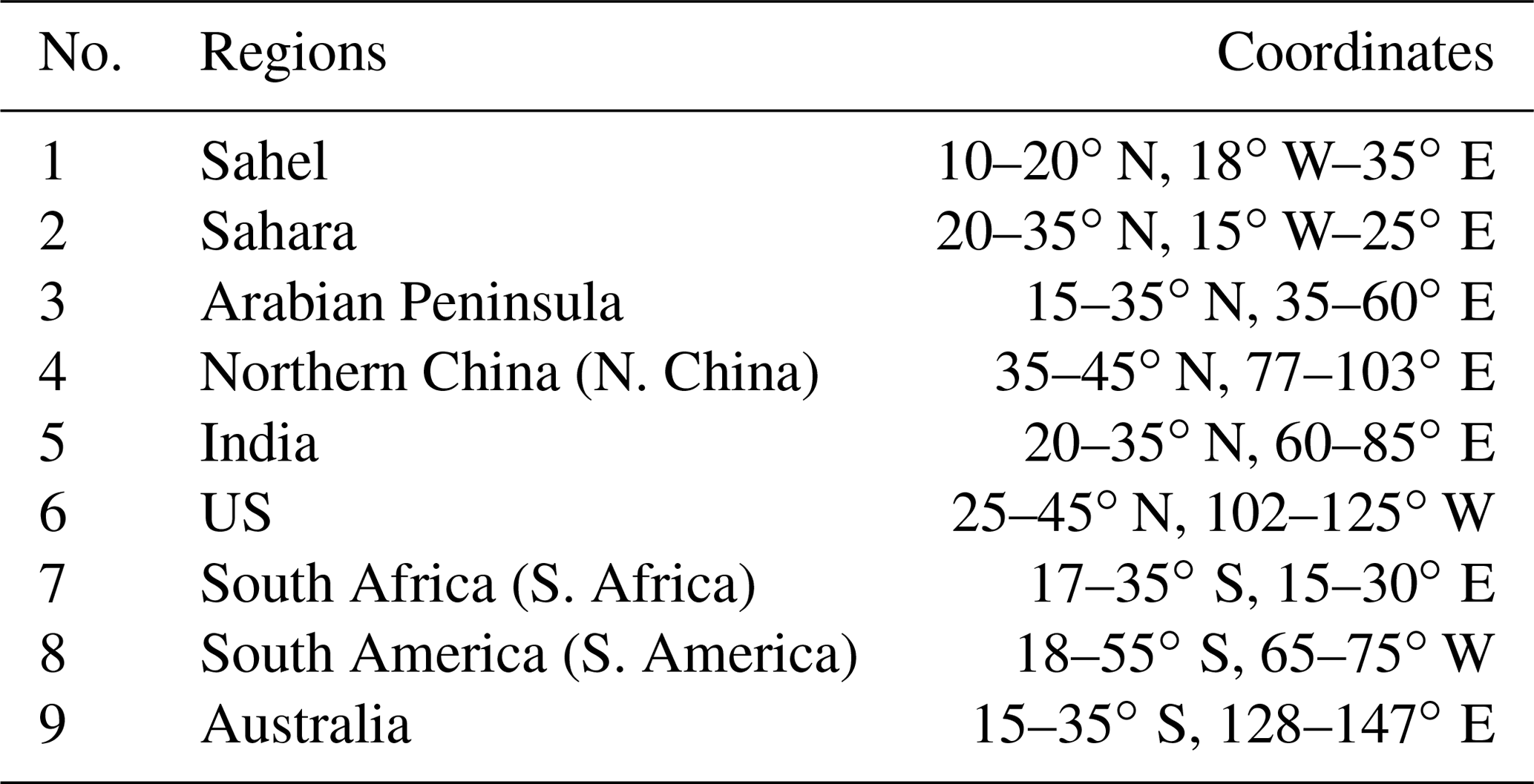
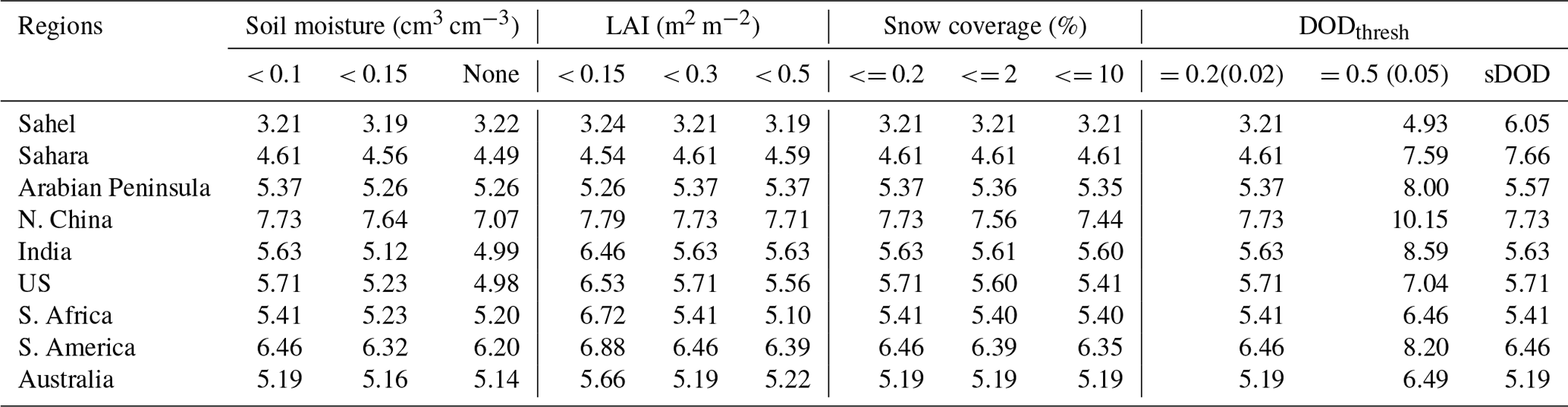
Table 2Sensitivity of the annual mean wind erosion threshold (m s−1) to the selection of different retrieval criteria. Note the setting of the last column is the same as DODthresh=0.2 or 0.02, except surface DOD (sDOD) from Aqua is used over northern Africa. Here DODthresh=0.2 or 0.5 is applied to dusty regions, i.e., the Sahel, Sahara, Arabian Peninsula, northern China, and India, while DODthresh=0.02 or 0.05 is applied to less dusty regions, i.e., the US, South Africa, South America, and Australia.
2.3 Sensitivities of Vthreshold to retrieval criteria and the selection of reanalysis surface winds
Table 2 shows variations in derived annual mean Vthreshold averaged in nine dust source regions (see Table 1 for locations) following slight changes of retrieval criteria: soil moisture, LAI, snow coverage, and DODthresh. When the soil moisture threshold is changed from 0.1 to 0.15 cm3 cm−3 or without the soil moisture constraint, the variations in Vthreshold are quite small, ranging from 0.01 to about 0.73 m s−1 (Table 2). Similarly, changes of LAI criteria from 0.15 to 0.5 m2 m−2 or snow coverage from 0.2 % to 10 % slightly change Vthreshold – within 1 m s−1 over most regions. On the other hand, Vthreshold is quite sensitive to the selection of DODthresh. Vthreshold would increase about 1 to 3 m s−1 if using DODthresh=0.5 for dusty regions (0.05 for less dusty regions) instead of DODthresh=0.2 (or 0.02). For instance, using DODthresh=0.5 increases the averaged annual mean Vthreshold over the Sahara from 4.6 m s−1 (using DODthresh=0.2) to about 7.6 m s−1.
As mentioned earlier, dust event frequency can be overestimated in regions with a high ratio of transported dust, and consequently Vthreshold would be underestimated. Here we provide a rough estimation about the influence of transported dust on Vthreshold over northern Africa. It is hard to separate local dust emission and transported dust in the column-integrated DOD, so we use surface DOD data (sDOD, Juliette Paireau, unpublished data), i.e., DOD from the surface to about 400 m, to approximate the component of DOD due to local emission. sDOD is derived by using the DOD vertical profile from the Cloud-Aerosol Lidar with Orthogonal Polarization (CALIOP; Winker et al., 2004., 2007) to first calculate a ratio of near-surface DOD (0–400 m) to total DOD (0–12 km) and then multiplying the ratio with daily MODIS Aqua DOD over northern Africa from 2003 to 2014. Using sDOD, Vthreshold over the Sahel would increase from 3.2 to 6.0 m s−1, while over the Sahara, Vthreshold would increase from 4.6 to 7.7 m s−1 (Table 2, last column).
Table 3Sensitivity of the annual mean wind erosion threshold (m s−1) to surface wind speeds from different reanalyses (DODthresh=0.2 or 0.02).

How Vthreshold would change when using surface winds from different reanalyses is examined in Table 3. Surface winds from the ERA-Interim product produce higher Vthreshold values than the NCEP1 product by 0.2 to 2.2 m s−1. Using surface winds from ERA5 also would increase Vthreshold by 1 to 1.6 m s−1 over northern Africa and about 1.5 m s−1 over Australia but create smaller differences in other regions.
In short, Vthreshold is less sensitive to small changes in the criteria to define a favorable, dry, and sparsely vegetated land surface condition for wind erosion than the choices of DODthresh or surface wind speeds from different reanalysis products. Over northern Africa, not separating transported dust from total DOD may lead to an underestimation of Vthreshold up to 3 m s−1 based on a rough estimation. However, due to the large uncertainties in quantifying transported dust and the regional converge of the sDOD dataset, we chose not to incorporate the results from sDOD to the global Vthreshold.
2.4 Simulation design
We will examine if the observation-constrained, spatially and temporally varying Vthreshold would improve dust simulation in GFDL AM4.0/LM4.0. AM4.0/LM4.0 is a coupled land–atmosphere model newly developed at GFDL (Zhao et al., 2018a, b). It uses the recent version of the GFDL Finite-Volume Cubed-Sphere dynamical core (FV3; Putman and Lin, 2007), which was developed for weather and climate applications with both hydrostatic and non-hydrostatic options. Some substantial updates have been incorporated into AM4.0, such as an updated version of the model radiation transfer code, an alternate topographic gravity wave drag formulation, a double-plume model representing shallow and deep convection, a “light” chemistry mechanism, and modulation on aerosol wet removal by convection and frozen precipitation (Zhao et al., 2018a, b). Here we used a model version with 33 vertical levels (with a model top at 1 hPa) and cube sphere with 192×192 grid boxes per cube face (approximately 50 km grid size).
The aerosol physics is based in large part on that of GFDL AM3.0 (Donner et al., 2011), but it has a simplified chemistry where ozone climatology from AM3.0 simulation (Naik et al., 2013) is prescribed. AM4.0 simulates the mass distribution of five aerosols: sulfate, black carbon, organic carbon, dust, and sea salt. Dust is partitioned into five size bins based on radius: 0.1–1 µm (bin 1), 1–2 µm (bin 2), 2–3 µm (bin 3), 3–6 µm (bin 4), and 6–10 µm (bin 5). The dust emission scheme follows the parameterization of Ginoux et al. (2001), as shown in the following equation:
where Fp is the flux of dust of particle size class p, C is a scaling factor with a unit of µg s2 m−5, here C is set to , S is the source function based on topographic depressions (Ginoux et al., 2001), sp is fraction of each size class, and V10 m is the surface 10 m wind speed, and Vt=6 m s−1 is the threshold of wind erosion.
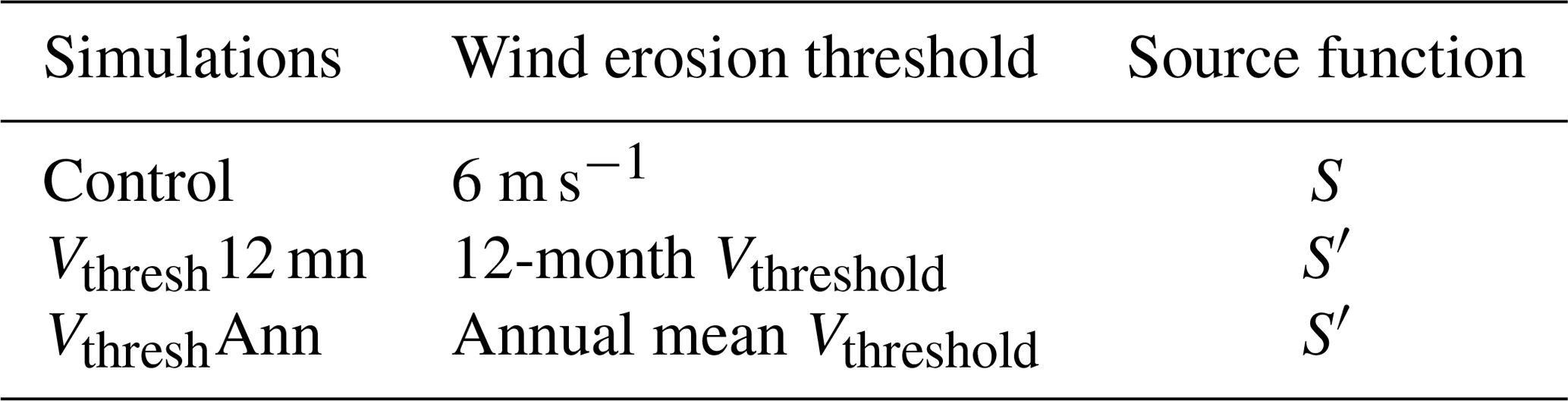
Three simulations with prescribed sea surface temperature (SST) and sea ice (Table 4) were conducted from 1999 to 2015, with the first year discarded for spin up. The Atmospheric Model Intercomparison Project-style (AMIP-style) SST and sea ice data (Taylor et al., 2000) are from the Program for Climate Model Diagnosis and Intercomparison (PCMDI), which combined HadISST (Hadley Centre Global Sea Ice and Sea Surface Temperature; Rayner et al., 2003) from the UK Met Office before 1981 and NCEP Optimum Interpolation (OI) v2 SST (Reynolds et al., 2002) afterwards. The surface winds in the simulations are nudged toward the NCEP1 reanalysis with a relaxation timescale of 6 h (Moorthi and Suarez, 1992). Note that the nudged surface winds are actually weaker than the surface wind speed simulated by the standard version of AM4.0/LM4.0 without nudging, so the overall magnitude of dust emission is lower than the standard version. Here we choose not to retune the dust emission scheme but instead test the usage of Vthreshold, which theoretically provides a more physics-based way to improve dust simulation. We also choose to keep the tuning factor C (Eq. 4) the same in all simulations to better examine the effects of implementing the newly developed Vthreshold.
In the Control run, the default model setting is used for dust emission, with a prescribed 6 m s−1 threshold of wind erosion (cf. Ginoux et al., 2019). In the Vthresh12 mn simulation, the observation-based climatological monthly Vthreshold is used to replace the constant wind erosion threshold. The default source function S in Eq. (4) only allows dust emission over bare ground by masking out regions with vegetation cover. Since LAI masking is already applied in the retrieval of Vthreshold (i.e., LAI < 0.3), we choose to use a source function that is the same as the default source function S but without vegetation masking, i.e., S′ (Fig. S2 in the Supplement). This allows the influence of the spatial and temporal variations in Vthreshold to be fully examined. The combination of source function S′ and Vthreshold also extends dust source from bare ground to sparsely vegetated areas as outlined by Vthreshold, e.g., over central North America, central India, and part of Australia, and that can increase dust emission in these regions. The pattern of extended dust source area largely resembles the vegetated dust source identified by Ginoux et al. (2012; their Fig. 15b) and Kim et al. (2013; their Fig. 9). All the other settings are the same as the Control run. The VthreshAnn simulation is the same as the Vthresh12 mn but uses the annual mean Vthreshold for each month. Since the same SST and sea ice are prescribed for all simulations and land use dose not change much during the short duration of simulation, the differences in simulated dynamic vegetation by LM4.0 among the three simulations are actually very small and can be ignored (see Figs. S3–S4 in the Supplement).
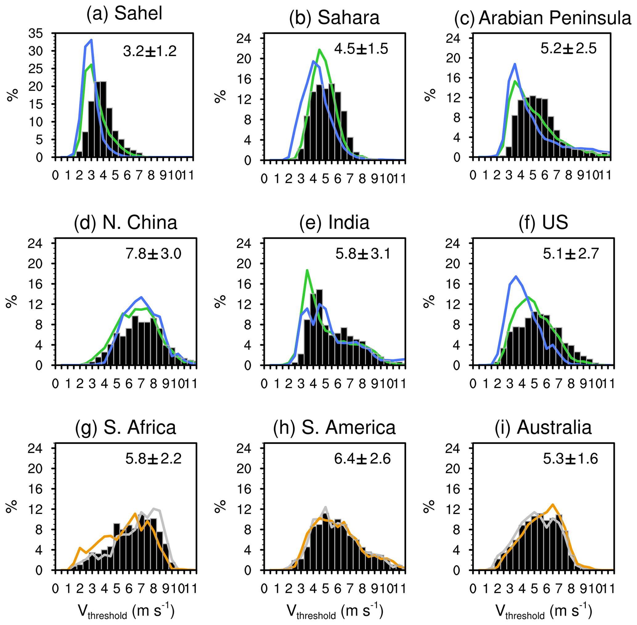
Figure 2(a–i) Frequency distribution of annual mean Vthreshold (black bars) in each region (black boxes in Fig. 1) and Vthreshold for dusty seasons, i.e., MAM (green) and JJA (blue) for regions in the Northern Hemisphere and SON (orange) and DJF (grey) for regions in the Southern Hemisphere. The mean (averaged over all grid points in the region, without area weight) and ± 1 standard deviation of Vthreshold in each region are shown on the top right of each plot.
3.1 Thresholds of wind erosion with DODthresh=0.2 (or 0.02) and DODthresh=0.5 (or 0.05)
Figure 1f–j show the derived threshold of wind erosion for each season and annual mean using DODthresh=0.2 (or 0.02). The seasonal variations in the wind erosion threshold are largely due to the variations in DOD and surface wind frequency distributions that are in turn associated with variations in land surface features, such as soil moisture, soil temperature, snow cover, and vegetation coverage in each month. Vthreshold is generally lower in MAM (March–April–May) and JJA (June–July–August) (SON (September–October–November) and DJF (December–January–February)) for Northern (Southern) Hemisphere dusty regions than in other seasons, consistent with higher FoO in these seasons. Vthreshold values are also lower in regions with a high FoO (Fig. 1a–e).
The distributions of Vthreshold for the annual mean (black bars) and dusty seasons (color lines; MAM and JJA for the Northern Hemisphere and SON and DJF for the Southern Hemisphere) for each dust source region (see Fig. 1f and Table 1 for locations) are shown in Fig. 2a–i. In the Sahel and Sahara, the annual mean Vthreshold peaks around 4 and 4.5–5.5 m s−1, respectively (Fig. 2a–b). This magnitude is lower than indicated from previous studies based on station observations in the region, e.g., Helgren and Prospero (1987) found the threshold velocity over eight stations in northwestern Africa ranged from 6.5 to 13 m s−1 during summer in 1974. Chomette et al. (1999) and Marsham et al. (2013) also reported higher wind erosion thresholds around 6–9 m s−1 at individual stations. On the other hand, Cowie et al. (2014) found that the annual threshold of wind erosion at the 25 % level, i.e., when surface condition is favorable for dust emission, can be lower than 6 m s−1 at some sites in the Sahel (their Fig. 5). Several factors may contribute to the discrepancies. Firstly, studies suggest that reanalysis datasets may underestimate surface wind speed in spring and for monsoon days in Africa (e.g., Largeron et al., 2015), and therefore they could lead to a lower value of Vthreshold than that derived from station observations. In fact, Bergametti et al. (2017) found even 3-hourly wind speed records at stations may miss short events with a high wind speed. As shown in Table 3, among the reanalysis wind products tested here, NCEP1 actually produced a lower Vthreshold in northern Africa than the other two reanalyses. Secondly, using the DOD frequency to approximate dust emission may lead to an overestimation of dust emission over regions such as the southern Sahel where transported dust is a large component and consequently an underestimation of Vthreshold. Based on our rough estimation, Vthreshold in northern Africa can be underestimated by up to 3 m s−1 (Sect. 2.3). In addition, different analysis time periods or methods to retrieve the wind erosion threshold may also contribute to the differences.
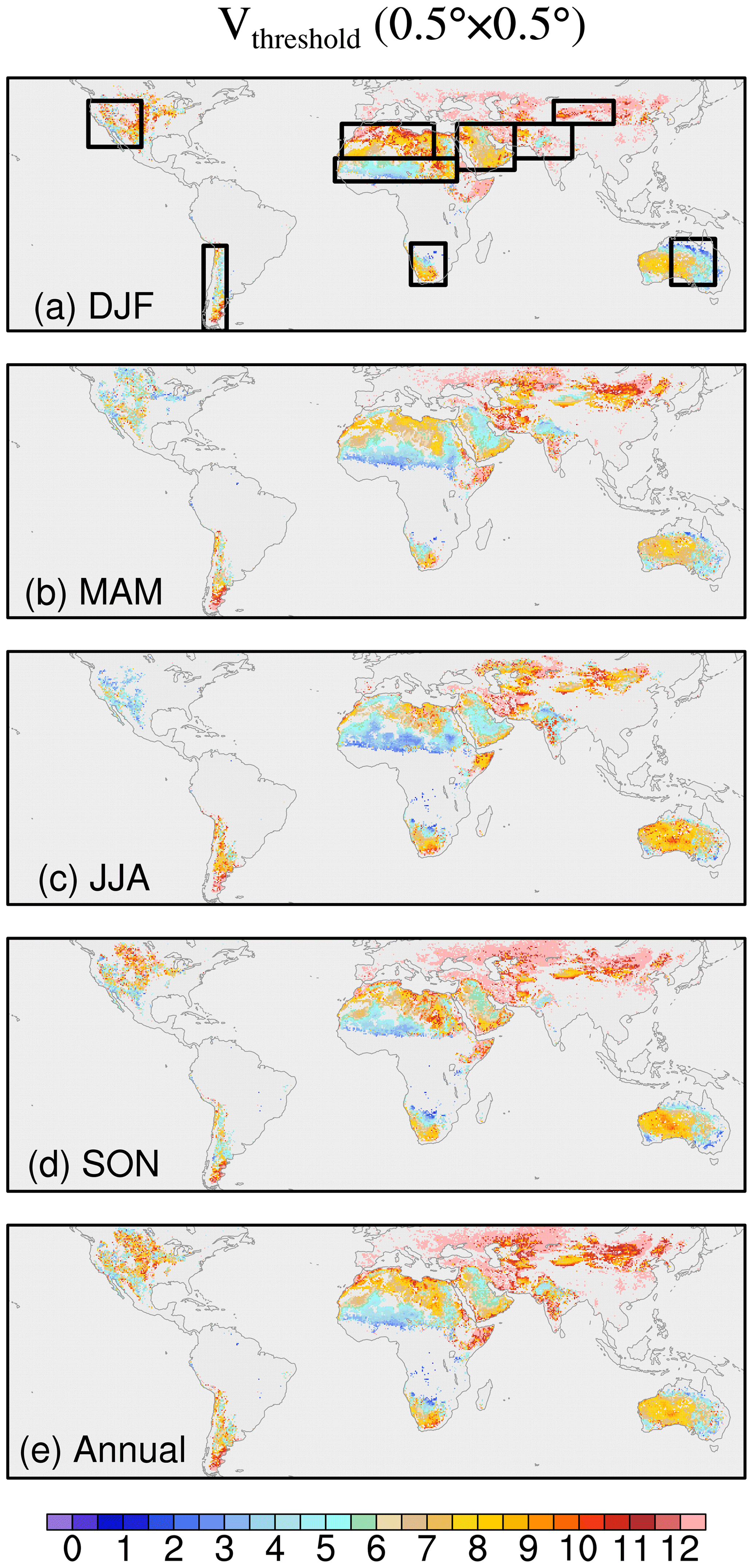
Figure 3(a–e) Threshold of wind erosion (Vthreshold; unit: m s−1) derived from satellite products and reanalyses for each season and the annual mean using DODthresh=0.5 (or 0.05). Black boxes in (a) denote nine dust source regions as listed in Table 1.
The annual mean Vthreshold in the Arabian Peninsula is a bit higher, with mean values at 5.2 m s−1 (Fig. 2c). The Vthreshold over northern China is even higher, with an annual mean of 7.8 m s−1. This is consistent with the results of Kurosaki and Mikami (2007), who found that under favorable land surface conditions the threshold wind speed ranges from 4.4±0.6 m s−1 in the Taklimakan Desert to 6.9±1.2 m s−1 over the Loess Plateau and around 9.8±1.6 m s−1 in the Gobi Desert. These values are also consistent with Ginoux and Deroubaix (2017) who found that the regional mean wind erosion threshold over northern China ranges from 6.5 to 9.1 m s−1. In India, the Vthreshold peaks at about 4.5 m s−1 and 6.5 m s−1, respectively (Fig. 2e). The second peak is probably related to anthropogenic dust sources over the central Indian subcontinent (Ginoux et al., 2012). We also note that in the Northern Hemisphere, Vthreshold in dusty seasons is shifted towards lower values than the annual mean (blue and green lines in Fig. 2a–f), but it is similar to the annual mean in the Southern Hemisphere (especially South America and Australia), indicating stronger influences of surface variability in the Northern Hemisphere.
Figure 3 shows the seasonal mean and annual mean global Vthreshold using DODthresh=0.5 (or 0.05). The corresponding distribution of annual mean Vthreshold in each region is shown in Fig. S5 in the Supplement. The derived Vthreshold is generally higher than using DODthresh=0.2 (or 0.02), especially over northern Africa, the Arabian Peninsula, India, and Asia (Fig. 3 and Table 2). The results are thus closer to previous station-based studies over northern Africa. On the other hand, over northern China, Vthreshold is around or greater than 8 m s−1 (Fig. 3e), slighter higher than previous estimates (e.g., Kurosaki and Mikami, 2007; Ginoux and Deroubaix, 2017).
In the following section, we will exam if the spatially and temporally varying Vthreshold would improve model simulation of the DOD spatial pattern, seasonal variations, frequency distribution, and surface dust concentrations in the GFDL AM4.0/LM4.0. Results using Vthreshold with DODthresh=0.2 (or 0.02) are shown in Sect. 3.2–3.3, and results using Vthreshold with DODthresh=0.5 (or 0.05) are briefly discussed in Sect. 4.
3.2 Vthreshold in the GFDL AM4.0/LM4.0 model
In this section we analyze the model output using the default setting (Control; Table 4), 12-month (Vthresh12 mn), and annual mean Vthreshold (VthreshAnn) by comparing model results with multiple observational datasets and MODIS DOD.
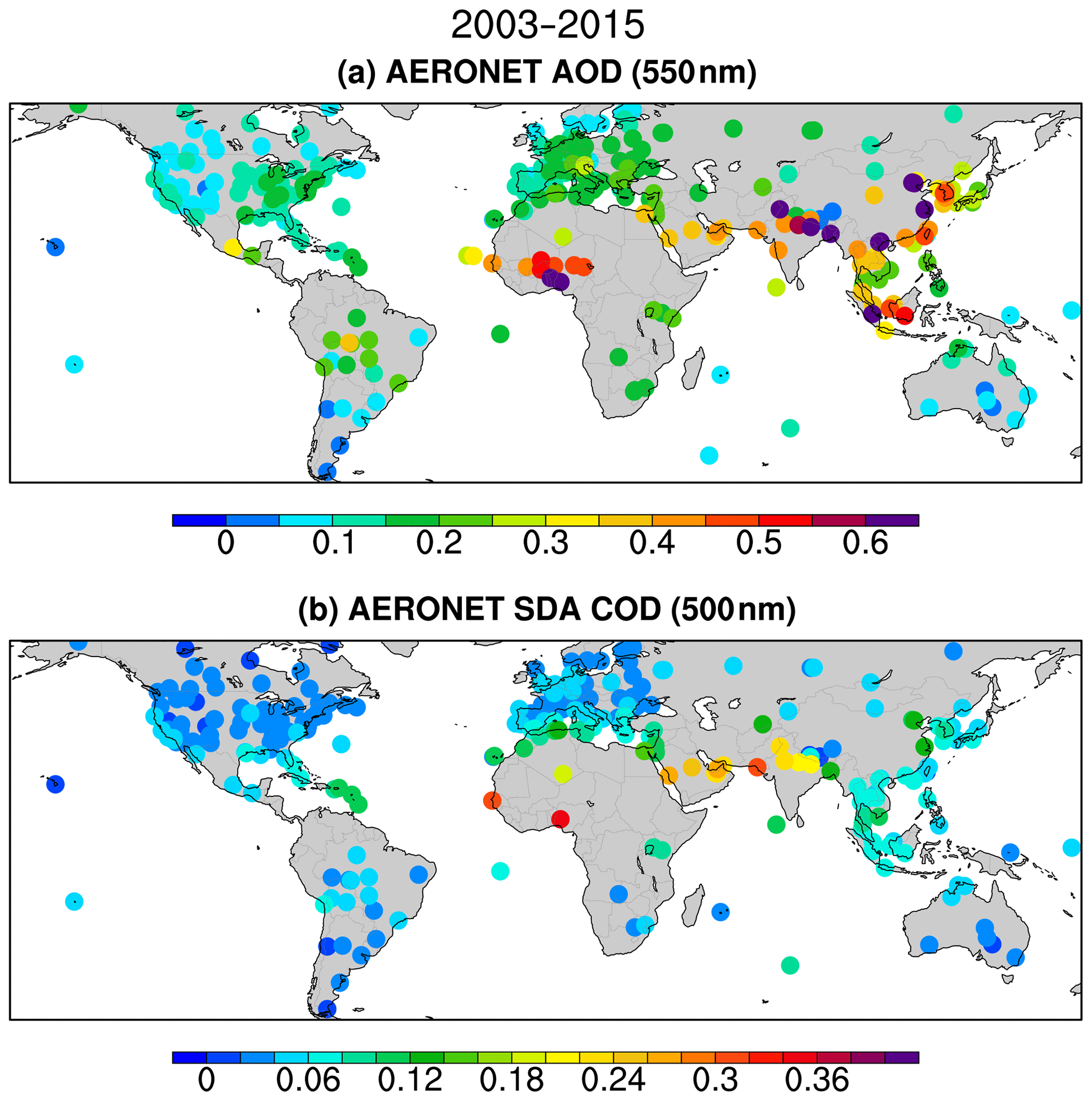
Figure 4Climatology of annual mean AERONET (a) AOD (550 nm) and (b) SDA COD (500 nm) averaged over 2003–2015.
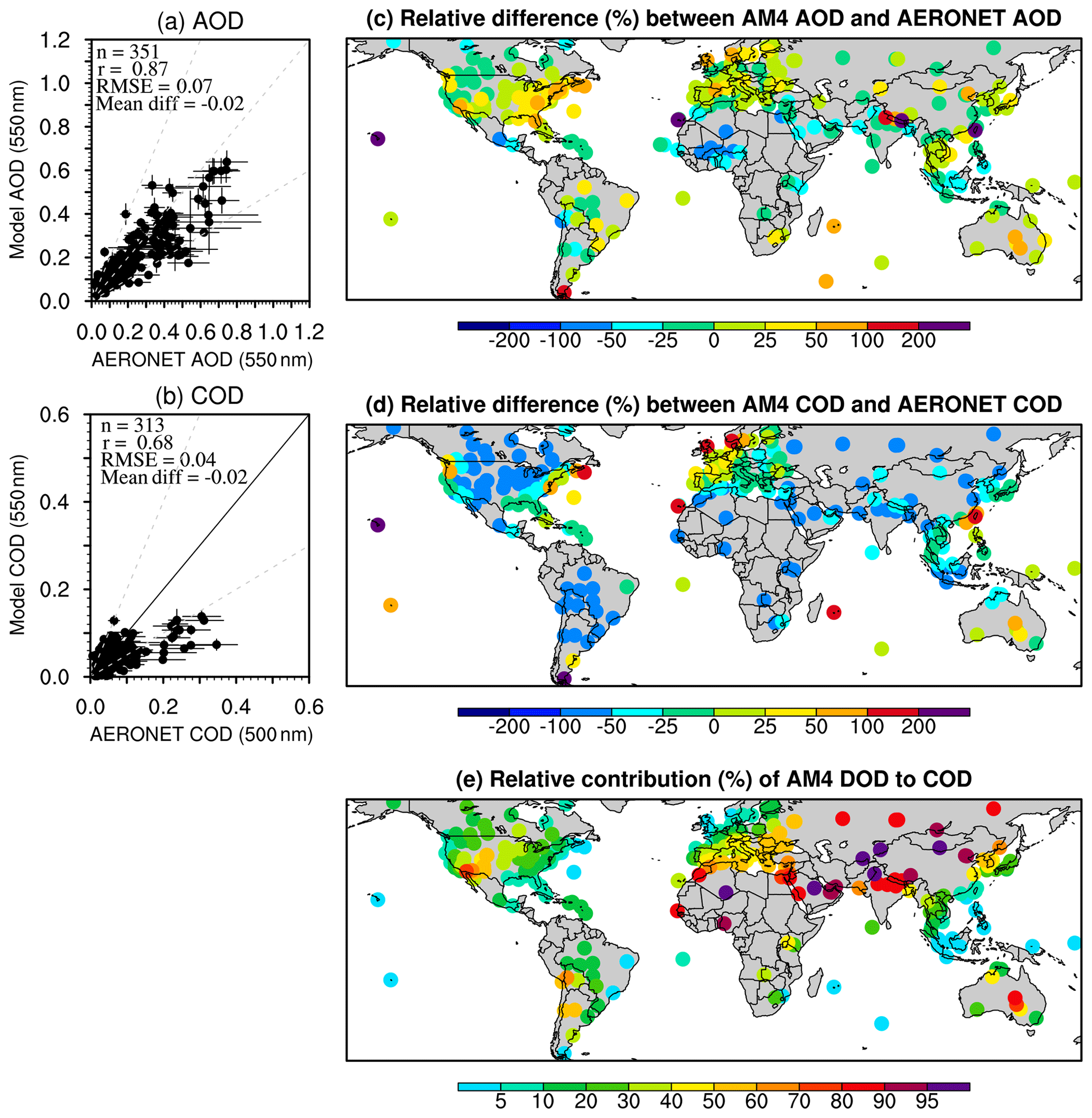
Figure 5Scatter plot of simulated annual mean (a) AOD and (b) COD in the Control run versus AERONET AOD and COD (a, b). The relative difference (as a percentage) (c) between modeled AOD and AERONET AOD and (d) between modeled COD and AERONET COD (c–e). (e) The relative contribution of DOD to COD in the model.
3.2.1 Climatology of AOD and DOD
In order to compare the model results with observations, we first show the climatology of AERONET AOD and COD from 2003 to 2015. The length of records for each station is shown in Fig. S6 in the Supplement. As shown in Fig. 4, annual mean global AOD is highest over Africa, the Arabian Peninsula, the Indian subcontinent, and southeastern Asia. In the latter two regions, high sulfate concentrations (e.g., Ginoux et al., 2006) and organic carbon from biomass burning in southeastern Asia (e.g., Lin et al., 2014) contribute substantially to the total AOD. The SDA COD shows the optical depth due to coarse aerosols, which includes both dust and sea salt, and sea salt over coastal regions or islands can be a major contributor. Here, high values (> 0.2) are largely located over dusty regions such as northern Africa, the Arabian Peninsula, and northern India (Fig. 4b).
Figure 5a–b show the scatter plots of modeled AOD and COD in the Control run versus AERONET AOD and COD, respectively. Here column-integrated extinction from both dust and sea salt is used to calculated COD in the model. The relative differences (as a percentage) between AM4.0 output and AERONET station data are also shown (Fig. 5c–d). The percentage of DOD to total COD in the model is displayed at the bottom (Fig. 5e). The simulated AOD is lower than that from AERONET over northern Africa, the Middle East, and western India, largely due to low values of COD simulated in these regions (Fig. 5d). Besides these regions, the COD over North America, South America, South Africa, and northern Eurasia is also, for the most part, underestimated by the model. Dust is the dominant contributor to the COD value over most of these low COD regions, except over central-to-eastern North America and central South America (Fig. 5e).
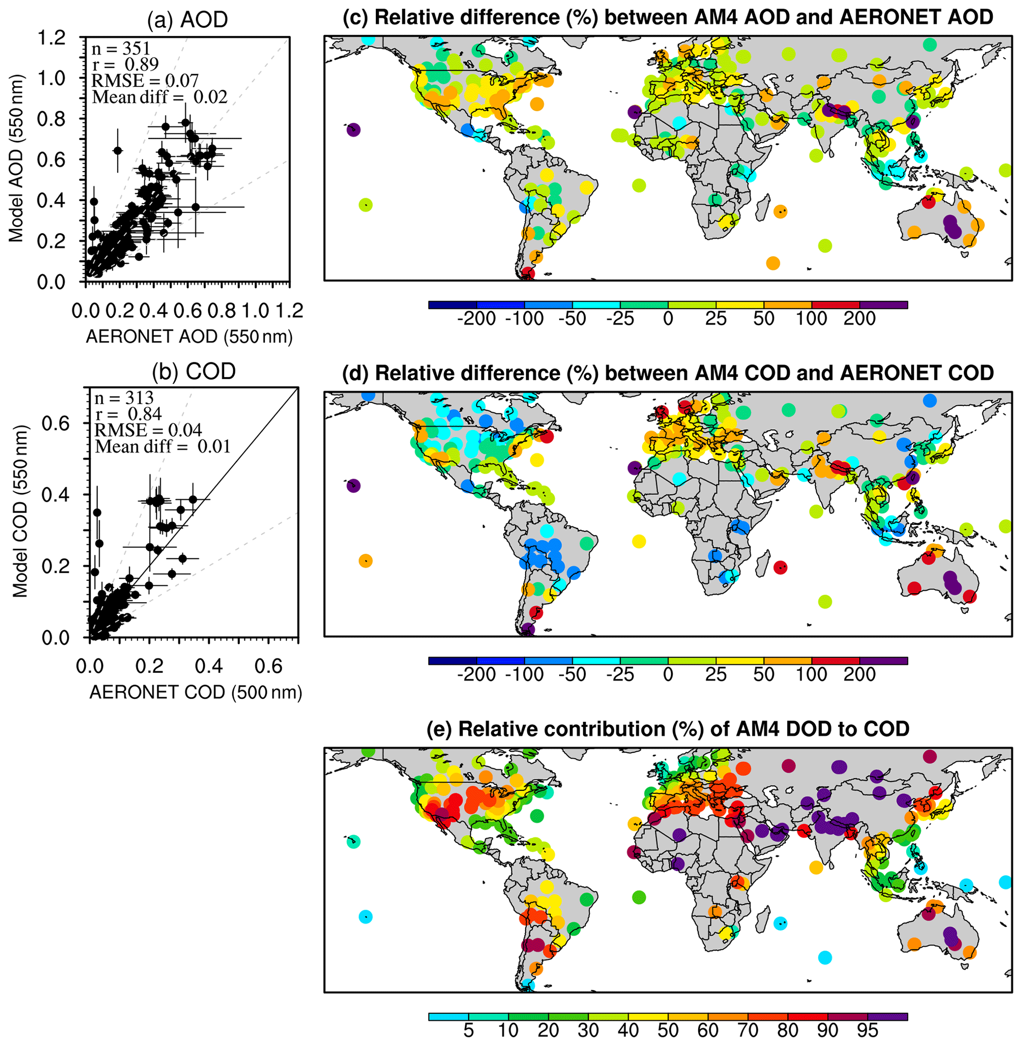
Figure 6Same as Fig. 5 but for the Vthresh12 mn simulation.
COD (and effectively DOD given its dominance in most regions) was better simulated in the subsequent model run using a prescribed 12-month Vthreshold in terms of both magnitude and spatial pattern. Figure 6 shows the results from the Vthresh12 mn simulation. COD is better captured, while the AOD effectively moves from a negative to a slightly positive bias (Fig. 6a–d). Most sites over northern Africa and the Middle East show a relatively small difference with AERONET COD (Fig. 6d). Over the Indian subcontinent, COD is overestimated, while over North America, excluding the east coast, northern Eurasia, and part of South America, COD is also better captured than in the Control run.
These improvements are largely associated with a better simulation of DOD in the “dust belt” (i.e., northern Africa and the Middle East). Figure 7 shows the DOD at 550 nm derived from AERONET AOD (see methodology for details) versus that from the Vthresh12 mn simulation. Over most stations in the Sahel, Mediterranean coasts, and central Middle East, the relative differences between modeled and observed DOD is within ±25 %.
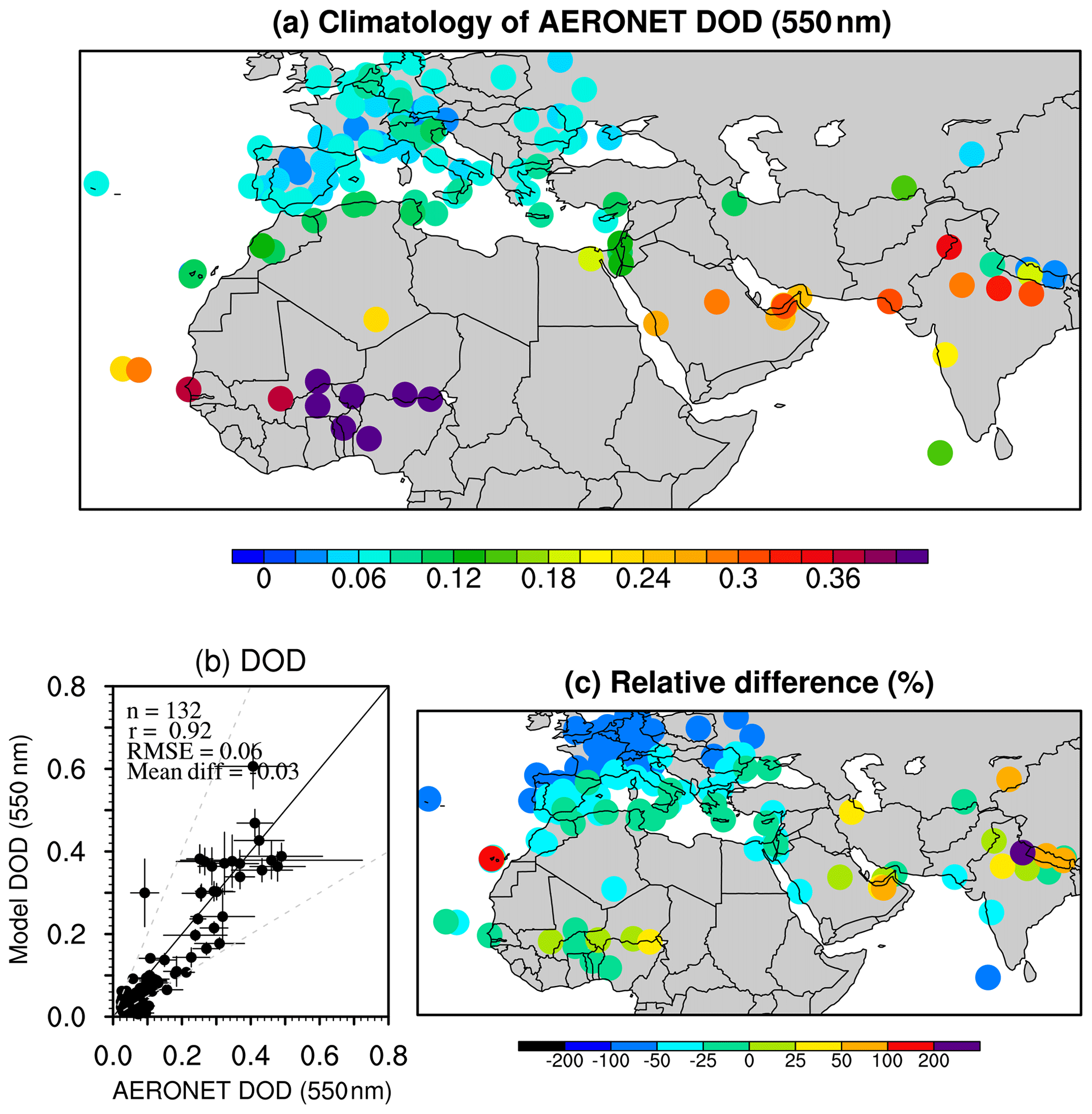
Figure 7(a) Climatology (2003–2015) of AERONET DOD (550 nm) over major dusty regions and (b) scatter plot of modeled DOD in the Vthresh12 mn simulation versus AERONET DOD. (c) The relative difference (as a percentage) between modeled DOD and AERONET DOD in the Vthresh12 mn simulation.
Figure 8 shows the regionally averaged annual mean DOD over nine dusty regions from MODIS and three simulations. The Control run largely underestimates DOD in all regions, while the magnitude of DOD is better captured in the Vthresh12 mn and VthreshAnn simulations, although slightly overestimated in the Sahel and greatly overestimated over Australia. In general, DOD simulated by the VthreshAnn run using a constant annual mean Vthreshold is higher than that simulated by the Vthresh12 mn run, consistent with the higher dust emission in the VthreshAnn run (Table S2 in the Supplement). Lack of the soil moisture constraint in the model, which is a very important element in capturing the variation of DOD in Australia (Evans et al., 2016), may contribute to the large overestimation of DOD in Australia.
3.2.2 Climatology of surface dust concentration
While DOD is a key parameter associated with the climate impact of dust, surface dust concentration is an important factor affecting local air quality. Here we compare the modeled surface dust concentration with RSMAS station observations. Model output is averaged from 2000 to 2015 to form the annual climatology. Consistent with the DOD output, the Control run largely underestimates surface dust concentrations at almost all of the sites (except sites 9 and 15; Fig. 9, top panel). The underestimation is reduced in the VthreshAnn simulation (Fig. 9, middle panel), with seven stations having model/observation ratios between 0.5 and 2 (white triangles). Over the coastal US (e.g., sites 16 and 13), dust concentrations are overestimated, consistent with the overestimation of DOD over the US and the Sahel (Fig. 8). Dust concentrations in Australia and the east coast of China are also overestimated by more than fivefold. Surface dust concentration is further improved in the Vthresh12 mn simulation (Fig. 9, bottom), with eight stations showing a model/observation ratio between 0.5 and 2 and only four stations overestimating or underestimating dust concentrations by more than 5 times.
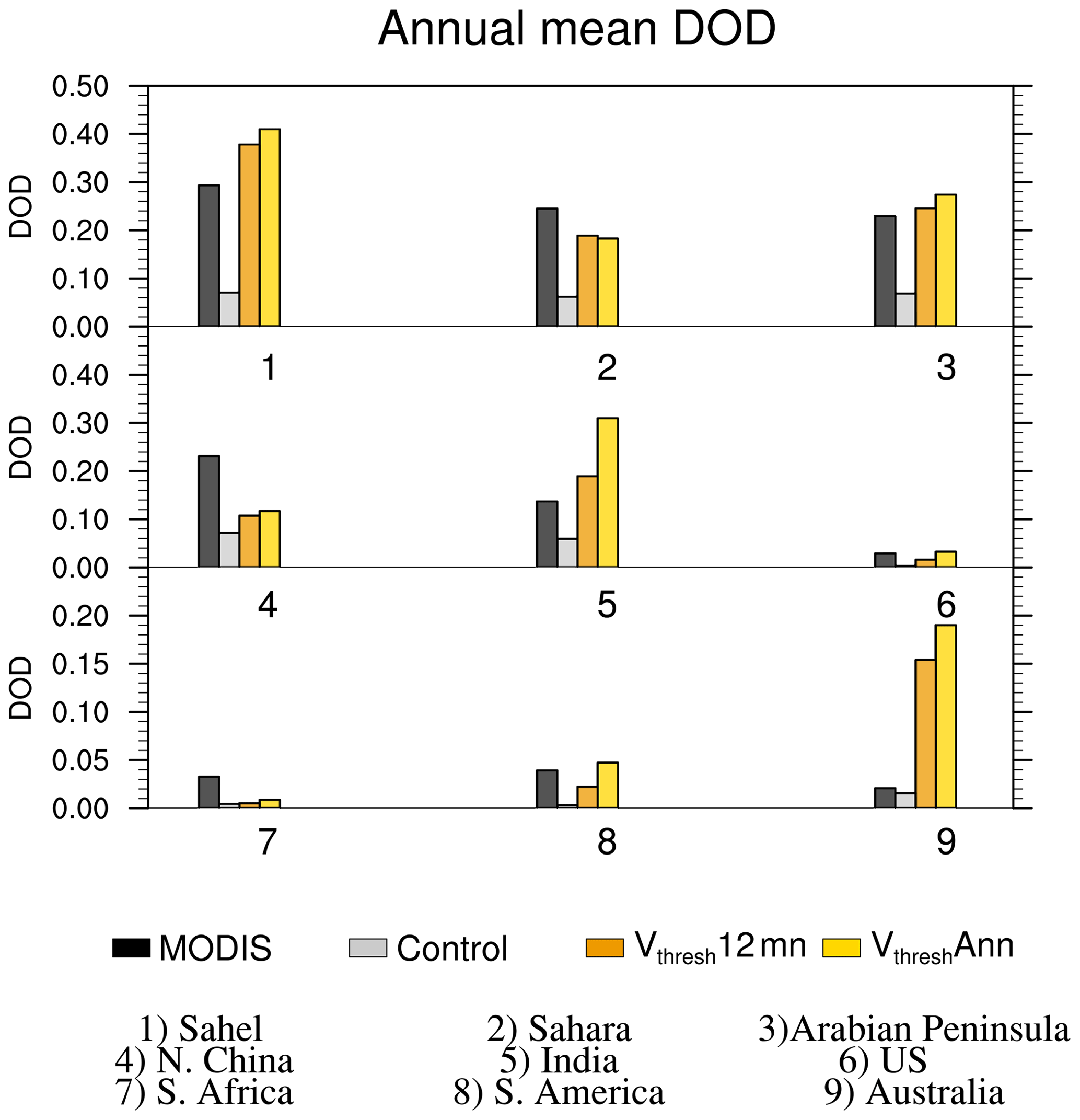
Figure 8Regionally averaged annual mean DOD (2003–2015) over nine regions from the Control (grey), Vthresh12 mn (orange), and VthreshAnn (yellow) simulations and MODIS (black).
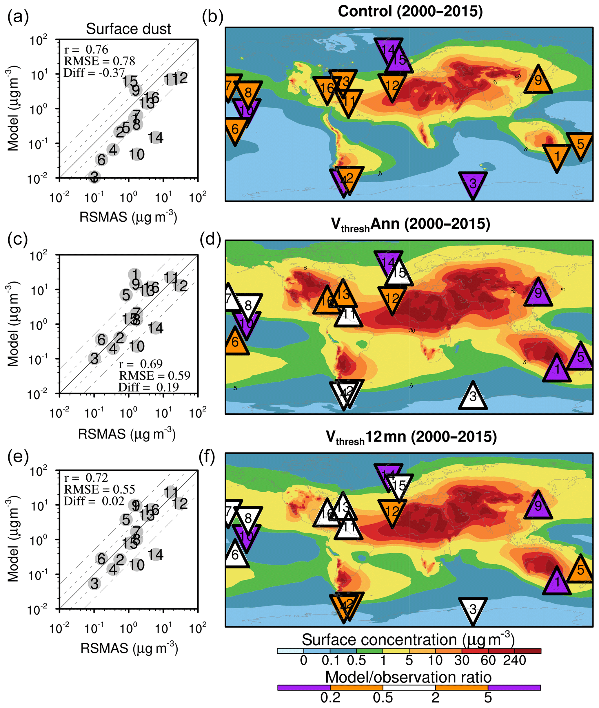
Figure 9Scatter plots (a, c, e) of model simulated (from top to bottom are the Control, VthreshAnn, and Vthresh12 mn simulations) surface dust concentration (µg m−3) versus the climatology of observed surface dust concentration from RSMAS stations (Savoie and Prospero, 1989). Spatial pattern of surface dust concentration from model output (shading; b, d, f) and the ratio between modeled and RSMAS station observed surface dust concentration (color triangles, with upward triangles indicating overestimation and downward triangles indicating underestimation). A total of 16 stations were used, and the numbers in each triangle (b, d, f) and grey dots (a, c, e) indicate the stations. The one–one, one–two, and one–five lines are plotted in solid, dashed, and dash-dotted lines in the scatter plots. Statistics in the scatter plots are calculated in logarithmic space.
Simulated surface fine dust concentration (calculated as dust bin dust bin 2) in the US is compared with gridded IMPROVE data (Fig. 10). While the Control run largely underestimates surface fine dust concentration, the simulated concentration is overall too high in the VthreshAnn run. The spatial pattern of fine dust concentration is better captured in the Vthresh12 mn run, with higher values over the southwestern US, but the magnitude is still overestimated, and additional dust hot spots are simulated over the northern Great Plains and the Midwest, which are not shown in the IMPROVE data. Such an overall overestimation may be attributed to a lack of soil moisture modulation in the dust emission scheme. The way in which dust bins are partitioned in the model can add uncertainties to model's representation of surface fine dust concentrations as well. On the other hand, the relatively low spatial coverage of IMPROVE sites over the northern Great Plains and Midwest (e.g., Pu and Ginoux, 2018a) may also add uncertainties to the data itself.
3.2.3 Seasonal cycles
Figure 11 compares the seasonal cycle of DOD from three simulations with MODIS DOD in nine dusty regions. The seasonal cycle of gridded AERONET COD (as an approximation of DOD; on a 0.5 × 0.5∘ grid) is also shown. Since the gridded COD may have large uncertainties over regions with only a few stations, such as the Sahel, Sahara, northern China, and South Africa, MODIS DOD is used as the main reference in the comparison. Seasonal cycles are better captured by the Vthresh12 mn simulation in the Sahel, the Sahara, and the Arabian Peninsula (Fig. 11a–c), although the spring and summer peak in the Sahel is overestimated, and the winter minimum in the Sahara is underestimated. The MAM peak of MODIS DOD in northern China is missed by both Vthresh12 mn and VthreshAnn simulations (Fig. 11d), while the JJA peak over India is largely overestimated (Fig. 11e). Over the US dusty region, the seasonal cycle in the Vthresh12 mn simulation is slightly underestimated compared to MODIS DOD but overestimated from May to August in the VthreshAnn simulation (Fig. 11f). DOD is underestimated in South Africa in all three simulations (Fig. 11g). Over South America, the peak from October to February is roughly captured by the Vthresh12 mn run but is overestimated by the VthreshAnn run (Fig. 11h). The seasonal cycles of DOD in Australia are very similar in all three simulations and largely resemble that in MODIS, although both the Vthresh12 mn and VthreshAnn simulations overestimate the DOD by about an order of magnitude.
Figure 12 shows the seasonal cycle of COD from 12 AERONET SDA sites over northern Africa and nearby islands (see Fig. S7 in the Supplement for site locations) along with MODIS DOD and DOD simulated in three runs. The magnitude of AERONET COD and MODIS DOD in these sites are very similar, despite missing values at sites 1, 4, 5, 8, and 11 and a smaller value at site 2 in MODIS. Over most of the sites, the seasonal cycle is better captured in the Vthresh12 mn and VthreshAnn simulations than the Control run, although the peak over Cairo_EMA_2 (site 12) is slightly underestimated, which is consistent with the underestimation of annual mean DOD in the area (Fig. 7).
We also examined the seasonal cycle of PM10 surface concentration at three Sahelian INDAAF stations (see Fig. S7 in the Supplement for site locations) from the LISA project. Figure 13a–c show PM10 surface dust concentration (here dust dominates total PM10 concentration) from the Control, Vthresh12 mn, and VthreshAnn simulations versus observed PM10 concentrations from three LISA sites. PM10 concentrations in these sites peak during boreal winter and spring and reach minima from July to September. These seasonal variations are associated with the dry northerly Harmattan wind in boreal winter and spring that transports Saharan dust southward to the Guinean coast and the scavenging effect of monsoonal rainfall in boreal summer that removes surface dust (Marticorena et al., 2010; Fiedler et al., 2015). While the Control run does not capture the seasonal cycles in these sites, the Vthresh12 mn run largely captures the spring peak and summer minimum, although the magnitude is overestimated. In all three sites, the simulated concentration in the VthreshAnn run is larger than that in the Vthresh12 mn run, especially from boreal fall to early spring. Such an overestimation is probably due to the prescribed constant annual mean Vthreshold, which is lower than it would be during the less dusty season (i.e., boreal fall to winter) and thus increases dust emission and surface concentrations.
Figure 13d–f show the seasonal cycle of DOD from three AERONET sites co-located with LISA INDAAF stations and from three simulations. The Vthresh12 mn and VthreshAnn simulations largely captured the seasonal cycle of DOD at these sites. The overestimation of near-surface PM10 dust concentrations (Fig. 13a–c) and the generally well-captured column-integrated DOD (Fig. 13d–f) indicate that the model likely underestimates dust concentration in the atmospheric column above the surface, which needs further investigation in future studies.
3.2.4 A dust storm over the US northern Great Plains on 18 October 2012
Can the AM4.0/LM4.0 with the prescribed Vthreshold better represent individual dust events? Here we examine a major dust storm captured by a MODIS Aqua true color image on 18 October 2012 (https://earthobservatory.nasa.gov/images/79459/dust-storm-in-the-great-plains, last access: November 2018) over the US northern Great Plains. There was a severe drought in 2012 with anomalously low precipitation centered over the central US (e.g., Hoerling et al., 2014). The dry conditions favored dust storm development when there were intensified surface winds. However, this storm was not predicted by the forecast models, such as the Goddard Earth Observing System version 5 (GEOS-5; Rienecker et al., 2008) and Navy Aerosol Analysis Prediction System (NAAPS; Witek et al., 2007; Reid et al., 2009; Westphal et al., 2009).
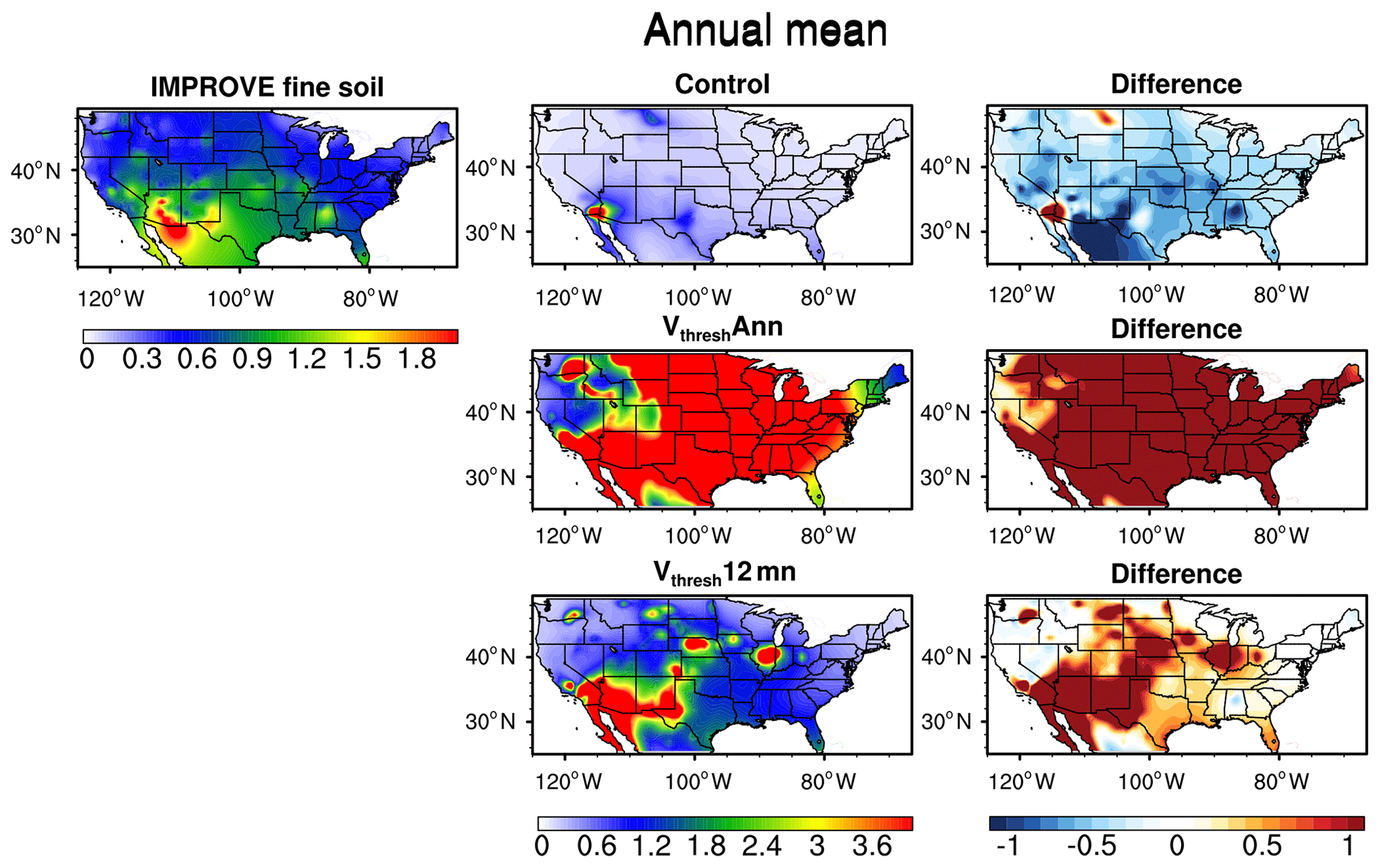
Figure 10Annual mean surface fine dust concentration (µg m−3) from IMPROVE stations (left column), three simulations (middle column), and the differences between model and observation (right column) for 2002–2015.

Figure 11Seasonal cycle of DOD from MODIS (black), the Control (grey), Vthresh12 mn (orange), and VthreshAnn (yellow) runs, with gridded AERONET SDA COD (blue) averaged over nine regions. The annual mean of each dataset in each region is listed on the top of the plot. Note that in (i) DOD from the Vthresh12 mn and VthreshAnn simulations is multiplied by 0.1 for clarity.

Figure 12Seasonal cycle of DOD over 12 AERONET SDA sites (see Fig. S7 in the Supplement for locations) from the Control (grey), Vthresh12 mn (orange), and VthreshAnn (yellow) simulations, along with DOD from MODIS (blue) and COD from AERONET (black dotted line). All values are averaged over 2003–2015. The location (coordinates) and the name (due to space, only the first seven characters are shown) of the sites are listed at the top of each plot.
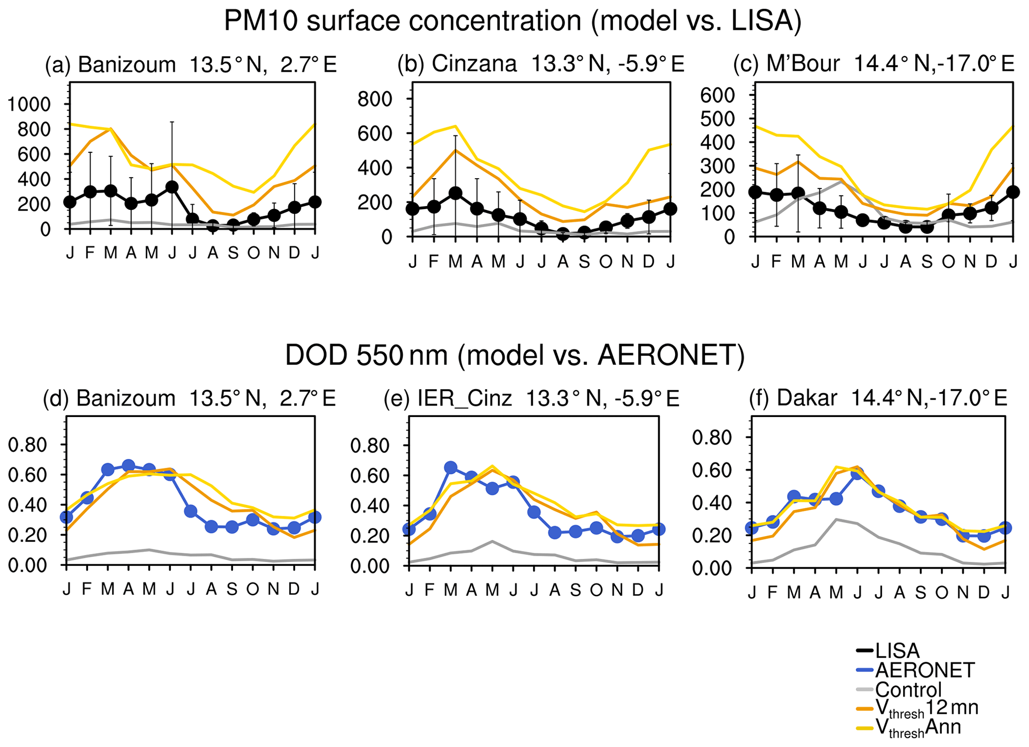
Figure 13(a–c) Seasonal cycle of PM10 surface concentration (black) over three sites from the LISA project, along with PM10 surface dust concentration from the Control (grey), Vthresh12 mn (orange), and VthreshAnn (yellow) simulations. Error bars are ± 1 standard deviation of the daily mean in each month averaged over 2006–2014 (units: µg m−3). (d–f) Seasonal cycle of DOD (550 nm) from three AERONET sites co-located with LISA sites (blue) versus that modeled by the Control (grey), Vthresh12 mn (orange), and VthreshAnn (yellow) simulations.
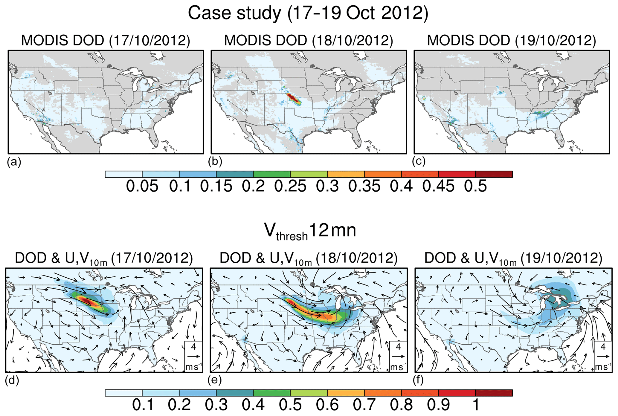
Figure 14(a–c) Daily DOD from MODIS. (d–f) Daily DOD simulated by the Vthresh12 mn run along with anomalies (with reference to the 2000–2015 mean) of surface wind vectors (m s−1) from 17 October to 19 October 2012. Only DOD over land is shown. Missing values in MODIS DOD (a–c) are plotted in grey shading.
As shown in Fig. 14, MODIS DOD captures this event, with a peak value above 0.5 over southwest Nebraska and northern Kansas on 18 October 2012. The Vthresh12 mn run also largely captures this event (Fig. 14, bottom panel), although the Control run totally misses it (not shown). In the model, the dust storm appears in South Dakota and Nebraska on 17 October 2012, along with the anomalous southwesterly winds. It reaches a maximum on 18 October in association with intensified anomalous southwesterly winds at the surface and an anomalous low-pressure system at 850 hPa (Fig. S8 in the Supplement). Note that the modeled dust storm center is located a bit northeastward compared to the MODIS DOD pattern and it also has greater magnitude and covers a larger area. On 19 October both the anomalous low-pressure system and surface wind speeds weaken, and the dust storm dissipates, with slightly elevated DOD levels over a region extending over the lower Mississippi River basin and the Midwest. This is somewhat consistent with MODIS records, which also shows slightly higher DOD levels over Tennessee and northern Alabama on 19 October regardless of the large area of missing values.
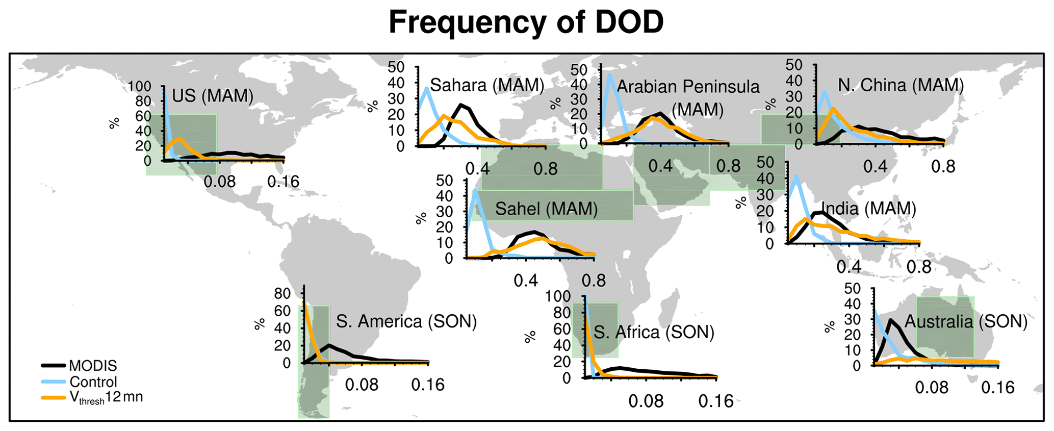
Figure 15Frequency distribution (as a percentage) of regionally averaged daily DOD from MODIS (black) versus that from the Control (light blue) and Vthresh12 mn (orange) simulations for the Sahara, the Sahel, the Arabian Peninsula, northern China, India, the western-to-central US, South America, South Africa, and Australia from 2003 to 2015. The x axis denotes the ranges of DOD (the bin spacing for dusty regions is 0.05 and for less dusty regions is 0.01), and the y axis is the percentage of occurrence. The light-green boxes denote the averaging areas. For regions in the Northern Hemisphere frequency in MAM is shown, while for regions in the Southern Hemisphere frequency in SON is shown.
3.3 Frequency distribution of DOD in the model versus that from MODIS
Figure 15 shows the frequency distribution of regional mean DOD during one dusty season (MAM in the Northern Hemisphere and SON in the Southern Hemisphere) for nine regions. Results from MODIS, the Control, and Vthresh12 mn runs are shown in black, blue, and orange lines, respectively. In most dusty regions, such as the Sahara, the Sahel, the Arabian Peninsula, India, and northern China, MODIS DOD frequency largely peaks between 0.2 to 0.4, while DOD frequency peaks at a much lower level between 0.02 to 0.08 in less dusty regions, such as the US, South America, South Africa, and Australia. This also justifies our selection of DODthresh of 0.02 (instead of 0.2) in the less dusty regions. The DOD distribution in the Control run is biased low and peaks around 0.05 in those dusty regions and between 0 and 0.01 in less dusty regions. The frequency is much better captured in the Vthresh12 mn run over the Arabian Peninsula and the Sahel, slightly improved but still biased low over the Sahara, northern China, India, and the US. The modeled frequency in the Vthresh12 mn run is biased high in Australia (peaks outside the maximum of the x axis, not shown) and shows little improvement over South Africa and South America. The overall improvement of DOD frequency using the time-varying 2-D Vthreshold occurs mostly over major dusty regions, which is consistent with the improvements in DOD climatology and seasonal cycle in the model simulations.
A global distribution of the threshold of wind erosion is retrieved using high-resolution MODIS DOD and land surface constraints from relatively high-resolution satellite products and reanalyses. While this climatological monthly Vthreshold provides useful information about the spatial and temporal variations in wind erosion threshold, there are some uncertainties associated with it. Here DOD frequency is derived using MODIS and other satellite products; thus the uncertainties in the satellite products are inherited in the derived DOD frequency distribution. Due to the cloud screening processes of MODIS products, dust activities over cloud-covered regions may be underestimated. Also, DOD frequency is derived based on daily observations over a 13-year record so that some variability of dust emission associated with alluvial sediments deposited by seasonal flooding may be not captured. Diurnal variability of dust emission and short-duration events such as haboobs are also not included. Since DOD is a column-integrated variable, it includes both locally emitted and remotely transported dust. When using DOD frequency distribution to approximate dust emission, it may overestimate dust emission in regions where transported dust is dominated and lead to an underestimation of Vthreshold. Future studies to better quantify the influences of transported dust are needed to further improve the quantitative retrieval of Vthreshold.
Previous studies found that over regions such as northern Africa, reanalysis products may underestimate surface wind speed in spring and monsoon seasons but overestimate it during dry nights (e.g., Largeron et al., 2015). This is largely because mechanisms such as density current that can enhance surface wind speed are not parameterized in the atmospheric models to produce the reanalysis products, while coarse spatial and temporal sampling may also contribute to the underestimation of reanalysis wind speeds. The selection of surface winds from different reanalysis products also affects the derived Vthreshold. Among the three reanalyses examined here, Vthreshold, derived from the NCEP1 reanalysis, shows slightly lower values than others.
In addition, Vthreshold is derived by matching the frequency distribution of DOD at certain levels (i.e., DODthresh) with the frequency distribution of daily maximum wind. An issue is that selecting a value of DODthresh is quite empirical. The influences of soil properties such as soil cohesion, particle size, and particle compositions on the threshold of wind erosion (e.g., Fécan et al., 1999; Alfaro and Gomes, 2001; Shao, 2001; Kok et al., 2014b) are not explicitly examined here and will need further investigation.
The influences of Vthreshold on AM4.0/LM4.0 results are twofold. On the one hand, it modifies the default constant threshold of wind erosion (Vt in Eq. 4) by allowing spatial and temporal variations of wind erosion threshold over bare ground, i.e., within the domain of default dust source function S (Fig. S9a–e in the Supplement). On the other hand, it slightly extends the potential emission area to sparsely vegetated regions as outlined by Vthreshold (Fig. S9f–j in the Supplement). Which effect dominates? Taking the Vthresh12 mn simulation as an example, Fig. S10 shows the differences of dust emission with the Control run. The increase of dust emission in the Vthresh12 mn simulation (also summarized in Table S2 in the Supplement) is largely associated with the enhanced emission over the bare ground (Fig. S10a–e in the Supplement), mainly over the regions with a reduced wind erosion threshold (Fig. S9a–e in the Supplement). The increased emission over sparsely vegetated areas over regions such as the southern Sahel, India, and Australia plays a minor role. This is consistent with Kim et al. (2013), who found that global dust emission in the Georgia Institute of Technology–Goddard Ozone Chemistry Aerosol Radiation and Transport (GOCART) model is dominated by emission from the bare ground.
The major benefit of using the spatially and temporally varying Vthreshold is that it improves the simulation of the DOD spatial pattern (Figs. 6–7), seasonal cycle (Figs. 11–13), and frequency distribution (Fig. 15) as well as the spatial pattern of surface dust concentrations (Figs. 9–10), which cannot be achieved by simply modifying the global tuning factor (i.e., C in Eq. 4) to fit the observations such as surface concentrations or optical depth.
The default setting in the Control run produced relatively low global dust emissions (978 Tg yr−1) in comparison with the Aerosol Comparisons between Observations and Models (AeroCom) multi-model median (1123 Tg yr−1; Huneeus et al., 2011) or a previous estimation based on MODIS DOD (1223 Tg yr−1; Ginoux et al., 2012). So we also conducted a test run (Control II) to increase global dust emission in the Control run to about 1232 Tg yr−1 by enlarging C in Eq. (4). The magnitude of DOD slightly increases, e.g., over the Sahel annual mean increases from 0.07 to 0.09; however, there is no improvement in terms of the seasonal cycle or spatial pattern, as expected.
We also examined the performance of Vthreshold using DODthresh=0.5 (or 0.05) in the AM4.0/LM4.0. Similarly, we conducted simulations with 12-month Vthreshold (Vthresh12 mn II) and annual mean Vthreshold (VthreshAnn II), all using the same tuning factor as in Control II. We found similar improvement in the DOD seasonal cycle and weaker improvement in the DOD spatial pattern and frequency distribution and surface dust concentrations (except with the IMPROVE data over the US and surface concentrations over the Sahel, where dust concentrations are previously overestimated). This is largely because higher Vthreshold leads to lower global dust emissions in the VthreshAnn II (1961 Tg yr−1) and Vthresh12 mn II simulations (1705 Tg yr−1) and overall lower DOD. Over the Mediterranean coast, Europe, and northern Asia, the DOD spatial pattern is not as well captured in the Vthresh12 mn II run as in the Vthreshold12 mn run, likely due to relatively high Vthreshold in these regions.
While dust aerosols play an important role in the Earth's climate system, large uncertainties exist in modeling its life cycle (e.g., Huneeus et al., 2011; Pu and Ginoux, 2018b). Constant thresholds of wind erosion are widely used in climate models for simplicity. Here, high-resolution MODIS Deep Blue dust optical depth and surface wind speeds from the NCEP1 reanalysis, along with other land surface factors that affect wind erosion, such as soil moisture, vegetation cover, snow cover, soil temperature, and soil depth, were used to develop a time-varying two-dimensional climatological threshold of wind erosion, Vthreshold, based on the seasonal variations of DOD and surface wind distribution frequencies. Vthreshold is generally lower in dusty seasons, i.e., MAM and JJA (SON and DJF) in the Northern (Southern) Hemisphere.
The climatological monthly Vthreshold was then incorporated into the GFDL AM4.0/LM4.0 model to examine the potential benefits relative to the use of a constant threshold. In comparison with the simulation using the default setting of a globally constant threshold of wind erosion (6 m s−1), both the magnitude of DOD and surface dust concentrations are increased and closer to observations. However, different from modifying the global tuning factor (i.e., C in Eq. 4) to increase the overall magnitudes of DOD or surface dust concentrations, we found the spatially and temporally varying Vthreshold largely improves the simulation of the spatial pattern, seasonal cycle, and frequency distribution of DOD over Northern Hemisphere dusty regions, such as northern Africa and the Arabian Peninsula, and slightly improves the simulation over India, the western-to-central US, and northern China. The seasonal cycle of DOD is also slightly improved in South America, although it changes little in South Africa. The incorporation of Vthreshold leads to an overestimation of DOD in Australia, likely in association with the absence of soil moisture constraints on dust emission in the model.
The spatial pattern of surface dust concentrations is also improved when spatially and temporally varying Vthreshold is incorporated. The fine dust concentration in the US is also better captured, with the maximum of the annual mean largely located over the southwestern US, although the magnitude is overestimated.
A constant annual mean Vthreshold is also tested in the model, and it is found to overestimate DOD over dusty seasons in the Arabian Peninsula, US, India, Australia, and South America. Surface PM10 concentrations in the Sahel during boreal fall and winter seasons are also largely overestimated with this setting. The results indicate the importance of including the seasonal cycle of Vthreshold in the model. Using time-varying 2-D Vthreshold, the model was also able to capture a strong dust storm in the US Great Plains in October 2012, which created deadly accidents, while some dust forecasting models failed to reproduce it.
Finally, this method to retrieve the global threshold of wind erosion can be conducted under different resolutions or surface wind reanalyses or applied to surface friction velocity datasets to match the resolution/scheme of dust models and may help improve their simulations and forecasting of dust distribution. As discussed in Sect. 4, there are uncertainties associated with this method, and future studies to better quantify the influence of transported dust to the overall DOD frequency distribution and incorporate station-based surface wind records into the retrieval process will further improve the dataset.
Both the monthly and annual mean Vthreshold data at a 0.5 × 0.5∘ resolution in NetCDF format are archived at https://www.gfdl.noaa.gov/pag-homepage/ (last access: December 2019, Pu and Ginoux, 2019).
The AERONET aerosol optical depth data and SDA data are available at https://aeronet.gsfc.nasa.gov/new_ web/download_all_ v3_ aod.html (last access: June 2018; Holben et al., 1998). IMPROVE fine dust data are available at http://views.cira.colostate.edu/fed/DataWizard/ (last access: March 2017, Malm et al., 1994; Hand et al., 2011). MODIS LAI data may be requested by contacting Ranga Myneni at Boston University.
PG and BP conceived the study. PG processed the MODIS Deep Blue aerosol data and guided model simulations. JP processed MODIS surface dust optical depth data. HG, SM, VN, ES, and MZ assisted with model configurations, while CH, JK, BM, NO, CP, and JMP provided guidance on data usage and analysis. BP conducted model simulations, analyzed data and model results, and wrote the paper with contributions from all other co-authors.
The authors declare that they have no conflict of interest.
This research is supported by NOAA and Princeton University's Cooperative Institute for Climate Science and NASA. The authors thank Veronica Chan and Hyeyum Shin for their helpful comments on the early version of this paper and Sophie Vandenbussche for her valuable suggestions. The helpful comments from two anonymous reviewers and the co-editor improved the paper. We also thank the AERONET program for establishing and maintaining the sun photometer sites used in this study and the IMPROVE network for the data. IMPROVE is a collaborative association of state, tribal, and federal agencies and international partners. The US Environmental Protection Agency is the primary funding source, with contracting and research support from the National Park Service. The Air Quality Group at the University of California, Davis is the central analytical laboratory, with ion analysis provided by the Research Triangle Institute and carbon analysis provided by the Desert Research Institute.
This research has been supported by NASA (grants no. NNH14ZDA001N-ACMAP and NNH16ZDA001NMAP).
This paper was edited by Yves Balkanski and reviewed by two anonymous referees.
Alfaro, S. C. and Gomes, L.: Modeling mineral aerosol production by wind erosion: Emission intensities and aerosol size distributions in source areas, J. Geophys. Res.-Atmos., 106, 18075–18084, https://doi.org/10.1029/2000jd900339, 2001.
Anderson, T. L., Wu, Y. H., Chu, D. A., Schmid, B., Redemann, J., and Dubovik, O.: Testing the MODIS satellite retrieval of aerosol fine-mode fraction, J. Geophys. Res.-Atmos., 110, D18204, https://doi.org/10.1029/2005jd005978, 2005.
Andrews, E., Ogren, J. A., Kinne, S., and Samset, B.: Comparison of AOD, AAOD and column single scattering albedo from AERONET retrievals and in situ profiling measurements, Atmos. Chem. Phys., 17, 6041–6072, https://doi.org/10.5194/acp-17-6041-2017, 2017.
Baddock, M. C., Ginoux, P., Bullard, J. E., and Gill, T. E.: Do MODIS-defined dust sources have a geomorphological signature?, Geophys. Res. Lett., 43, 2606–2613, https://doi.org/10.1002/2015gl067327, 2016.
Bangert, M., Nenes, A., Vogel, B., Vogel, H., Barahona, D., Karydis, V. A., Kumar, P., Kottmeier, C., and Blahak, U.: Saharan dust event impacts on cloud formation and radiation over Western Europe, Atmos. Chem. Phys., 12, 4045–4063, https://doi.org/10.5194/acp-12-4045-2012, 2012.
Barchyn, T. E. and Hugenholtz, C. H.: Comparison of four methods to calculate aeolian sediment transport threshold from field data: Implications for transport prediction and discussion of method evolution, Geomorphology, 129, 190–203, https://doi.org/10.1016/j.geomorph.2011.01.022, 2011.
Bentsen, M., Bethke, I., Debernard, J. B., Iversen, T., Kirkevåg, A., Seland, Ø., Drange, H., Roelandt, C., Seierstad, I. A., Hoose, C., and Kristjánsson, J. E.: The Norwegian Earth System Model, NorESM1-M – Part 1: Description and basic evaluation of the physical climate, Geosci. Model Dev., 6, 687–720, https://doi.org/10.5194/gmd-6-687-2013, 2013.
Bristow, C. S., Hudson-Edwards, K. A., and Chappell, A.: Fertilizing the Amazon and equatorial Atlantic with West African dust, Geophys. Res. Lett., 37, L14807, https://doi.org/10.1029/2010gl043486, 2010.
Cheng, T., Peng, Y., Feichter, J., and Tegen, I.: An improvement on the dust emission scheme in the global aerosol-climate model ECHAM5-HAM, Atmos. Chem. Phys., 8, 1105–1117, https://doi.org/10.5194/acp-8-1105-2008, 2008.
Chomette, O., Legrand, M., and Marticorena, B.: Determination of the wind speed threshold for the emission of desert dust using satellite remote sensing in the thermal infrared, J. Geophys. Res.-Atmos., 104, 31207–31215, https://doi.org/10.1029/1999jd900756, 1999.
Collins, W. J., Bellouin, N., Doutriaux-Boucher, M., Gedney, N., Halloran, P., Hinton, T., Hughes, J., Jones, C. D., Joshi, M., Liddicoat, S., Martin, G., O'Connor, F., Rae, J., Senior, C., Sitch, S., Totterdell, I., Wiltshire, A., and Woodward, S.: Development and evaluation of an Earth-System model – HadGEM2, Geosci. Model Dev., 4, 1051–1075, https://doi.org/10.5194/gmd-4-1051-2011, 2011.
Cook, B. I., Miller, R. L., and Seager, R.: Dust and sea surface temperature forcing of the 1930s ”Dust Bowl” drought, Geophys. Res. Lett., 35, L08710, https://doi.org/10.1029/2008gl033486, 2008.
Cook, B. I., Miller, R. L., and Seager, R.: Amplification of the North American ”Dust Bowl” drought through human-induced land degradation, P. Natl. Acad. Sci. USA, 106, 4997–5001, https://doi.org/10.1073/pnas.0810200106, 2009.
Cook, B. I., Seager, R., Miller, R. L., and Mason, J. A.: Intensification of North American Megadroughts through Surface and Dust Aerosol Forcing, J. Climate, 26, 4414–4430, https://doi.org/10.1175/Jcli-D-12-00022.1, 2013.
Cowie, S. M., Knippertz, P., and Marsham, J. H.: A climatology of dust emission events from northern Africa using long-term surface observations, Atmos. Chem. Phys., 14, 8579–8597, https://doi.org/10.5194/acp-14-8579-2014, 2014.
Dee, D. P., Uppala, S. M., Simmons, A. J., Berrisford, P., Poli, P., Kobayashi, S., Andrae, U., Balmaseda, M. A., Balsamo, G., Bauer, P., Bechtold, P., Beljaars, A. C. M., van de Berg, I., Biblot, J., Bormann, N., Delsol, C., Dragani, R., Fuentes, M., Greer, A. J., Haimberger, L., Healy, S. B., Hersbach, H., Holm, E. V., Isaksen, L., Kallberg, P., Kohler, M., Matricardi, M., McNally, A. P., Mong-Sanz, B. M., Morcette, J.-J., Park, B.-K., Peubey, C., de Rosnay, P., Tavolato, C., Thepaut, J. N., and Vitart, F.: The ERA-Interim reanalysis: Configuration and performance of the data assimilation system, Q. J. Roy. Meteorol. Soc., 137, 553–597, https://doi.org/10.1002/qj.828, 2011.
Donner, L. J., Wyman, B. L., Hemler, R. S., Horowitz, L. W., Ming, Y., Zhao, M., Golaz, J. C., Ginoux, P., Lin, S. J., Schwarzkopf, M. D., Austin, J., Alaka, G., Cooke, W. F., Delworth, T. L., Freidenreich, S. M., Gordon, C. T., Griffies, S. M., Held, I. M., Hurlin, W. J., Klein, S. A., Knutson, T. R., Langenhorst, A. R., Lee, H. C., Lin, Y. L., Magi, B. I., Malyshev, S. L., Milly, P. C. D., Naik, V., Nath, M. J., Pincus, R., Ploshay, J. J., Ramaswamy, V., Seman, C. J., Shevliakova, E., Sirutis, J. J., Stern, W. F., Stouffer, R. J., Wilson, R. J., Winton, M., Wittenberg, A. T., and Zeng, F. R.: The Dynamical Core, Physical Parameterizations, and Basic Simulation Characteristics of the Atmospheric Component AM3 of the GFDL Global Coupled Model CM3, J. Climate, 24, 3484–3519, https://doi.org/10.1175/2011jcli3955.1, 2011.
Draxier, R. R. and Hess, G. D.: An overview of the HYSPLIT_ 4 modelling system for trajectories, dispersion and deposition, Aust. Meteorol. Mag., 47, 295–308, 1998.
Draxler, R. R., Ginoux, P., and Stein, A. F.: An empirically derived emission algorithm for wind-blown dust, J. Geophys. Res.-Atmos., 115, D16212, https://doi.org/10.1029/2009jd013167, 2010.
Du, J., Jones, L. A., and Kimball, J. S.: Daily Global Land Parameters Derived from AMSR-E and AMSR2, Version 2, https://doi.org/10.5067/RF8WPYOPJKL2, 2017a.
Du, J., Kimball, J. S., Jones, L. A., Kim, Y., Glassy, J., and Watts, J. D.: A global satellite environmental data record derived from AMSR-E and AMSR2 microwave Earth observations, Earth Syst. Sci. Data, 9, 791–808, https://doi.org/10.5194/essd-9-791-2017, 2017b.
Dubovik, O. and King, M. D.: A flexible inversion algorithm for retrieval of aerosol optical properties from Sun and sky radiance measurements, J. Geophys. Res.-Atmos., 105, 20673–20696, https://doi.org/10.1029/2000jd900282, 2000.
Dumont, M., Brun, E., Picard, G., Michou, M., Libois, Q., Petit, J. R., Geyer, M., Morin, S., and Josse, B.: Contribution of light-absorbing impurities in snow to Greenland's darkening since 2009, Nat. Geosci., 7, 509–512, https://doi.org/10.1038/Ngeo2180, 2014.
Dunion, J. P. and Velden, C. S.: The impact of the Saharan air layer on Atlantic tropical cyclone activity, B. Am. Meteorol. Soc., 85, 353–366, https://doi.org/10.1175/Bams-85-3-353, 2004.
Eck, T. F., Holben, B. N., Reid, J. S., Dubovik, O., Smirnov, A., O'Neill, N. T., Slutsker, I., and Kinne, S.: Wavelength dependence of the optical depth of biomass burning, urban, and desert dust aerosols, J. Geophys. Res.-Atmos., 104, 31333–31349, https://doi.org/10.1029/1999jd900923, 1999.
Evan, A. T., Dunion, J., Foley, J. A., Heidinger, A. K., and Velden, C. S.: New evidence for a relationship between Atlantic tropical cyclone activity and African dust outbreaks, Geophys. Res. Lett., 33, L19813, https://doi.org/10.1029/2006gl026408, 2006.
Evan, A. T., Fiedler, S., Zhao, C., Menut, L., Schepanski, K., Flamant, C., and Doherty, O.: Derivation of an observation-based map of North African dust emission, Aeolian Res., 16, 153–162, https://doi.org/10.1016/j.aeolia.2015.01.001, 2015.
Evans, S., Ginoux, P., Malyshev, S., and Shevliakova, E.: Climate-vegetation interaction and amplification of Australian dust variability, Geophys. Res. Lett., 43, 11823–11830, https://doi.org/10.1002/2016gl071016, 2016.
Fécan, F., Marticorena, B., and Bergametti, G.: Parametrization of the increase of the aeolian erosion threshold wind friction velocity due to soil moisture for arid and semi-arid areas, Ann. Geophys.-Atm. Hydr., 17, 149–157, https://doi.org/10.1007/s005850050744, 1999.
Fiedler, S., Kaplan, M. L., and Knippertz, P.: The importance of Harmattan surges for the emission of North African dust aerosol, Geophys. Res. Lett., 42, 9495–9504, https://doi.org/10.1002/2015gl065925, 2015.
Fung, I. Y., Meyn, S. K., Tegen, I., Doney, S. C., John, J. G., and Bishop, J. K. B.: Iron supply and demand in the upper ocean, Global Biogeochem. Cy., 14, 281–295, https://doi.org/10.1029/1999gb900059, 2000.
Garrigues, S., Lacaze, R., Baret, F., Morisette, J. T., Weiss, M., Nickeson, J. E., Fernandes, R., Plummer, S., Shabanov, N. V., Myneni, R. B., Knyazikhin, Y., and Yang, W.: Validation and intercomparison of global Leaf Area Index products derived from remote sensing data, J. Geophys. Res.-Biogeo., 113, G02028, https://doi.org/10.1029/2007jg000635, 2008.
Gillette, D. A., Adams, J., Endo, A., Smith, D., and Kihl, R.: Threshold Velocities for Input of Soil Particles into the Air by Desert Soils, J. Geophys. Res.-Oceans, 85, 5621–5630, https://doi.org/10.1029/JC085iC10p05621, 1980.
Gillette, D. A. and Passi, R.: Modeling Dust Emission Caused by Wind Erosion, J. Geophys. Res.-Atmos., 93, 14233–14242, https://doi.org/10.1029/JD093iD11p14233, 1988.
Ginoux, P., Chin, M., Tegen, I., Prospero, J. M., Holben, B., Dubovik, O., and Lin, S. J.: Sources and distributions of dust aerosols simulated with the GOCART model, J. Geophys. Res.-Atmos., 106, 20255–20273, https://doi.org/10.1029/2000jd000053, 2001.
Ginoux, P., Horowitz, L. W., Ramaswamy, V., Geogdzhayev, I. V., Holben, B. N., Stenchikov, G., and Tie, X.: Evaluation of aerosol distribution and optical depth in the Geophysical Fluid Dynamics Laboratory coupled model CM2.1 for present climate, J. Geophys. Res.-Atmos., 111, D22210, https://doi.org/10.1029/2005jd006707, 2006.
Ginoux, P., Garbuzov, D., and Hsu, N. C.: Identification of anthropogenic and natural dust sources using Moderate Resolution Imaging Spectroradiometer (MODIS) Deep Blue level 2 data, J. Geophys. Res.-Atmos., 115, D05204, https://doi.org/10.1029/2009jd012398, 2010.
Ginoux, P., Prospero, J. M., Gill, T. E., Hsu, N. C., and Zhao, M.: Global-Scale Attribution of Anthropogenic and Natural Dust Sources and Their Emission Rates Based on MODIS Deep Blue Aerosol Products, Rev. Geophys., 50, RG3005, https://doi.org/10.1029/2012rg000388, 2012.
Ginoux, P. and Deroubaix, A.: Space observations of dust in East Asia, Air pollution in Eastern Asia: an integrated perspective, edited by: Bouarar, I., Wang, X., and Brasseur, G. P., Springer, 2017.
Ginoux, P., Malyshev, S., Shevliakova, E., Chan, H. G., Guo, H., Milly, C., Naik, V., Pascale, S., Paulot, F., Pu, B., Zhao, M., and Kapnick, S.: Distribution of absorbing aerosols in snow over high mountain ranges in GFDL AM4/LM4, in preparation, 2019.
Hand, J. L., Copeland, S. A., Day, D. E., Dillner, A. M., Indresand, H., Malm, W. C., McDade, C. E., Moore, C. T., Pitchford, M. L., Schichtel, B. A., and Watson, J. G.: IMPROVE (Interagency Monitoring of Protected Visual Environments): Spatial and seasonal patterns and temporal variability of haze and its constituents in the United States, available at: http://vista.cira.colostate.edu/Improve/spatial-and-seasonal-patterns-and-temporal-variability-of-haze-and-its-constituents-in-the-united-states-report-v-june-2011/ (last access: February 2019), 2011.
Hand, J. L., White, W. H., Gebhart, K. A., Hyslop, N. P., Gill, T. E., and Schichtel, B. A.: Earlier onset of the spring fine dust season in the southwestern United States, Geophys. Res. Lett., 43, 4001–4009, https://doi.org/10.1002/2016gl068519, 2016.
Hand, J. L., Gill, T. E., and Schichtel, B. A.: Spatial and seasonal variability in fine mineral dust and coarse aerosol mass at remote sites across the United States, J. Geophys. Res.-Atmos., 122, 3080–3097, https://doi.org/10.1002/2016jd026290, 2017.
Helgren, D. M. and Prospero, J. M.: Wind Velocities Associated with Dust Deflation Events in the Western Sahara, J. Clim. Appl. Meteorol., 26, 1147–1151, https://doi.org/10.1175/1520-0450(1987)026<1147:Wvawdd>2.0.Co;2, 1987.
Hersbach, H. and Dee, D.: ERA5 reanalysis is in production, ECMWF Newsletter, No. 147, 7 pp., 2016.
Hoerling, M., Eischeid, J., Kumar, A., Leung, R., Mariotti, A., Mo, K., Schubert, S., and Seager, R.: Causes and Predictability of the 2012 Great Plains Drought, B. Am. Meteorol. Soc., 95, 269–282, https://doi.org/10.1175/Bams-D-13-00055.1, 2014.
Holben, B. N., Eck, T. F., Slutsker, I., Tanre, D., Buis, J. P., Setzer, A., Vermote, E., Reagan, J. A., Kaufman, Y. J., Nakajima, T., Lavenu, F., Jankowiak, I., and Smirnov, A.: AERONET – A federated instrument network and data archive for aerosol characterization, Remote Sens. Environ., 66, 1–16, https://doi.org/10.1016/S0034-4257(98)00031-5, 1998.
Holben, B. N., Eck, T. F., Slutsker, I., Smirnov, A., Sinyuk, A., Schafer, J., Giles, D., and Dubovik, O.: AERONET's Version 2.0 quality assurance criteria, available at: https://aeronet.gsfc.nasa.gov/new_web/PDF/AERONETcriteria_final1.pdf (last access: February 2019), 2006.
Hsu, N. C., Tsay, S. C., King, M. D., and Herman, J. R.: Aerosol properties over bright-reflecting source regions, IEEE T. Geosci. Remote, 42, 557–569, https://doi.org/10.1109/Tgrs.2004.824067, 2004.
Hsu, N. C., Jeong, M. J., Bettenhausen, C., Sayer, A. M., Hansell, R., Seftor, C. S., Huang, J., and Tsay, S. C.: Enhanced Deep Blue aerosol retrieval algorithm: The second generation, J. Geophys. Res.-Atmos., 118, 9296–9315, https://doi.org/10.1002/jgrd.50712, 2013.
Huneeus, N., Schulz, M., Balkanski, Y., Griesfeller, J., Prospero, J., Kinne, S., Bauer, S., Boucher, O., Chin, M., Dentener, F., Diehl, T., Easter, R., Fillmore, D., Ghan, S., Ginoux, P., Grini, A., Horowitz, L., Koch, D., Krol, M. C., Landing, W., Liu, X., Mahowald, N., Miller, R., Morcrette, J.-J., Myhre, G., Penner, J., Perlwitz, J., Stier, P., Takemura, T., and Zender, C. S.: Global dust model intercomparison in AeroCom phase I, Atmos. Chem. Phys., 11, 7781–7816, https://doi.org/10.5194/acp-11-7781-2011, 2011.
Jickells, T. D., An, Z. S., Andersen, K. K., Baker, A. R., Bergametti, G., Brooks, N., Cao, J. J., Boyd, P. W., Duce, R. A., Hunter, K. A., Kawahata, H., Kubilay, N., laRoche, J., Liss, P. S., Mahowald, N., Prospero, J. M., Ridgwell, A. J., Tegen, I., and Torres, R.: Global iron connections between desert dust, ocean biogeochemistry, and climate, Science, 308, 67–71, https://doi.org/10.1126/science.1105959, 2005.
Jin, Q., Wei, J., Yang, Z.-L., Pu, B., and Huang, J.: Consistent response of Indian summer monsoon to Middle East dust in observations and simulations, Atmos. Chem. Phys., 15, 9897–9915, https://doi.org/10.5194/acp-15-9897-2015, 2015.
Jin, Q. J., Wei, J. F., and Yang, Z. L.: Positive response of Indian summer rainfall to Middle East dust, Geophys. Res. Lett., 41, 4068–4074, https://doi.org/10.1002/2014gl059980, 2014.
Jin, Q. J., Yang, Z. L., and Wei, J. F.: Seasonal Responses of Indian Summer Monsoon to Dust Aerosols in the Middle East, India, and China, J. Climate, 29, 6329–6349, https://doi.org/10.1175/Jcli-D-15-0622.1, 2016.
Jones, C. D., Hughes, J. K., Bellouin, N., Hardiman, S. C., Jones, G. S., Knight, J., Liddicoat, S., O'Connor, F. M., Andres, R. J., Bell, C., Boo, K.-O., Bozzo, A., Butchart, N., Cadule, P., Corbin, K. D., Doutriaux-Boucher, M., Friedlingstein, P., Gornall, J., Gray, L., Halloran, P. R., Hurtt, G., Ingram, W. J., Lamarque, J.-F., Law, R. M., Meinshausen, M., Osprey, S., Palin, E. J., Parsons Chini, L., Raddatz, T., Sanderson, M. G., Sellar, A. A., Schurer, A., Valdes, P., Wood, N., Woodward, S., Yoshioka, M., and Zerroukat, M.: The HadGEM2-ES implementation of CMIP5 centennial simulations, Geosci. Model Dev., 4, 543–570, https://doi.org/10.5194/gmd-4-543-2011, 2011.
Kalnay, E., Kanamitsu, M., Kistler, R., Collins, W., Deaven, D., Gandin, L.,
Iredell, M., Saha, S., White, G., Woollen, J., Zhu, Y., Chelliah, M.,
Ebisuzaki, W., Higgins, W., Janowiak, J., Mo, K. C., Ropelewski, C., Wang,
J., Leetmaa, A., Reynolds, R., Jenne, R., and Joseph, D.: The NCEP/NCAR
40-year reanalysis project, B. Am. Meteorol. Soc., 77, 437–471,
doi10.1175/1520-0477(1996)077<0437:Tnyrp>2.0.Co;2, 1996.
Kim, D., Chin, M. A., Bian, H. S., Tan, Q., Brown, M. E., Zheng, T., You, R. J., Diehl, T., Ginoux, P., and Kucsera, T.: The effect of the dynamic surface bareness on dust source function, emission, and distribution, J. Geophys. Res.-Atmos., 118, 8710–886, https://doi.org/10.1029/2012jd017907, 2013.
Kim, M. K., Lau, W. K. M., Kim, K. M., Sang, J., Kim, Y. H., and Lee, W. S.: Amplification of ENSO effects on Indian summer monsoon by absorbing aerosols, Clim. Dynam., 46, 2657–2671, https://doi.org/10.1007/s00382-015-2722-y, 2016.
Knippertz, P.: Dust emissions in the West African heat trough - the role of the diurnal cycle and of extratropical disturbances, Meteorol. Z., 17, 553–563, https://doi.org/10.1127/0941-2948/2008/0315, 2008.
Kok, J. F., Albani, S., Mahowald, N. M., and Ward, D. S.: An improved dust emission model – Part 2: Evaluation in the Community Earth System Model, with implications for the use of dust source functions, Atmos. Chem. Phys., 14, 13043–13061, https://doi.org/10.5194/acp-14-13043-2014, 2014a.
Kok, J. F., Mahowald, N. M., Fratini, G., Gillies, J. A., Ishizuka, M., Leys, J. F., Mikami, M., Park, M.-S., Park, S.-U., Van Pelt, R. S., and Zobeck, T. M.: An improved dust emission model – Part 1: Model description and comparison against measurements, Atmos. Chem. Phys., 14, 13023–13041, https://doi.org/10.5194/acp-14-13023-2014, 2014b.
Kurosaki, Y. and Mikami, M.: Effect of snow cover on threshold wind velocity of dust outbreak, Geophys. Res. Lett., 31, L03106, https://doi.org/10.1029/2003gl018632, 2004.
Kurosaki, Y. and Mikami, M.: Threshold wind speed for dust emission in east Asia and its seasonal variations, J. Geophys. Res.-Atmos., 112, D17202, https://doi.org/10.1029/2006jd007988, 2007.
Largeron, Y., Guichard, F., Bouniol, D., Couvreux, F., Kergoat, L., and Marticorena, B.: Can we use surface wind fields from meteorological reanalyses for Sahelian dust emission simulations?, Geophys. Res. Lett., 42, 2490–2499, https://doi.org/10.1002/2014gl062938, 2015.
Levin, Z., Ganor, E., and Gladstein, V.: The effects of desert particles coated with sulfate on rain formation in the eastern Mediterranean, J. Appl. Meteorol., 35, 1511–1523, https://doi.org/10.1175/1520-0450(1996)035<1511:Teodpc>2.0.Co;2, 1996.
Lin, C. Y., Zhao, C., Liu, X. H., Lin, N. H., and Chen, W. N.: Modelling of long-range transport of Southeast Asia biomass-burning aerosols to Taiwan and their radiative forcings over East Asia, Tellus B, 66, 23733, https://doi.org/10.3402/tellusb.v66.23733, 2014.
Mahowald, N. M., Baker, A. R., Bergametti, G., Brooks, N., Duce, R. A., Jickells, T. D., Kubilay, N., Prospero, J. M., and Tegen, I.: Atmospheric global dust cycle and iron inputs to the ocean, Global Biogeochem. Cy., 19, GB4025, https://doi.org/10.1029/2004gb002402, 2005.
Mahowald, N. M., Kloster, S., Engelstaedter, S., Moore, J. K., Mukhopadhyay, S., McConnell, J. R., Albani, S., Doney, S. C., Bhattacharya, A., Curran, M. A. J., Flanner, M. G., Hoffman, F. M., Lawrence, D. M., Lindsay, K., Mayewski, P. A., Neff, J., Rothenberg, D., Thomas, E., Thornton, P. E., and Zender, C. S.: Observed 20th century desert dust variability: impact on climate and biogeochemistry, Atmos. Chem. Phys., 10, 10875–10893, https://doi.org/10.5194/acp-10-10875-2010, 2010.
Malm, W. C., Sisler, J. F., Huffman, D., Eldred, R. A., and Cahill, T. A.: Spatial and Seasonal Trends in Particle Concentration and Optical Extinction in the United-States, J. Geophys. Res.-Atmos., 99, 1347–1370, https://doi.org/10.1029/93jd02916, 1994.
Marsham, J. H., Hobby, M., Allen, C. J. T., Banks, J. R., Bart, M., Brooks, B. J., Cavazos-Guerra, C., Engelstaedter, S., Gascoyne, M., Lima, A. R., Martins, J. V., McQuaid, J. B., O'Leary, A., Ouchene, B., Ouladichir, A., Parker, D. J., Saci, A., Salah-Ferroudj, M., Todd, M. C., and Washington, R.: Meteorology and dust in the central Sahara: Observations from Fennec supersite-1 during the June 2011 Intensive Observation Period, J. Geophys. Res.-Atmos., 118, 4069–4089, https://doi.org/10.1002/jgrd.50211, 2013.
Marticorena, B. and Bergametti, G.: Modeling the Atmospheric Dust Cycle – 1. Design of a Soil-Derived Dust Emission Scheme, J. Geophys. Res.-Atmos., 100, 16415–16430, https://doi.org/10.1029/95jd00690, 1995.
Marticorena, B., Bergametti, G., Aumont, B., Callot, Y., Ndoume, C., and Legrand, M.: Modeling the atmospheric dust cycle – 2. Simulation of Saharan dust sources, J. Geophys. Res.-Atmos., 102, 4387–4404, https://doi.org/10.1029/96jd02964, 1997.
Marticorena, B., Chatenet, B., Rajot, J. L., Traoré, S., Coulibaly, M., Diallo, A., Koné, I., Maman, A., NDiaye, T., and Zakou, A.: Temporal variability of mineral dust concentrations over West Africa: analyses of a pluriannual monitoring from the AMMA Sahelian Dust Transect, Atmos. Chem. Phys., 10, 8899–8915, https://doi.org/10.5194/acp-10-8899-2010, 2010.
Mbourou, G. N., Bertrand, J. J., and Nicholson, S. E.: The diurnal and seasonal cycles of wind-borne dust over Africa north of the equator, J. Appl. Meteorol., 36, 868–882, https://doi.org/10.1175/1520-0450(1997)036<0868:Tdasco>2.0.Co;2, 1997.
Miller, R. L. and Tegen, I.: Climate response to soil dust aerosols, J. Climate, 11, 3247–3267, https://doi.org/10.1175/1520-0442(1998)011<3247:Crtsda>2.0.Co;2, 1998.
Miller, R. L., Tegen, I., and Perlwitz, J.: Surface radiative forcing by soil dust aerosols and the hydrologic cycle, J. Geophys. Res.-Atmos., 109, D04203, https://doi.org/10.1029/2003jd004085, 2004.
Moorthi, S. and Suarez, M. J.: Relaxed Arakawa-Schubert – a Parameterization of Moist Convection for General-Circulation Models, Mon. Weather Rev., 120, 978–1002, https://doi.org/10.1175/1520-0493(1992)120<0978:Rasapo>2.0.Co;2, 1992.
Naik, V., Horowitz, L. W., Fiore, A. M., Ginoux, P., Mao, J. Q., Aghedo, A. M., and Levy, H.: Impact of preindustrial to present-day changes in short-lived pollutant emissions on atmospheric composition and climate forcing, J. Geophys. Res.-Atmos., 118, 8086–8110, https://doi.org/10.1002/jgrd.50608, 2013.
Nakajima, T., Higurashi, A., Kawamoto, K., and Penner, J. E.: A possible correlation between satellite-derived cloud and aerosol microphysical parameters, Geophys. Res. Lett., 28, 1171–1174, https://doi.org/10.1029/2000gl012186, 2001.
O'Neill, N. T., Eck, T. F., Smirnov, A., Holben, B. N., and Thulasiraman, S.: Spectral discrimination of coarse and fine mode optical depth, J. Geophys. Res.-Atmos., 108, 4559, https://doi.org/10.1029/2002jd002975, 2003.
O'rgill, M. and Sehmel, G.: Frequency and diurnal variation of dust storms in the contiguous USA, Atmos. Environ., 10, 813–825, 1976.
Painter, T. H., Deems, J. S., Belnap, J., Hamlet, A. F., Landry, C. C., and Udall, B.: Response of Colorado River runoff to dust radiative forcing in snow, P. Natl. Acad. Sci. USA, 107, 17125–17130, https://doi.org/10.1073/pnas.0913139107, 2010.
Painter, T. H., Skiles, S. M., Deems, J. S., Brandt, W. T., and Dozier, J.: Variation in Rising Limb of Colorado River Snowmelt Runoff Hydrograph Controlled by Dust Radiative Forcing in Snow, Geophys. Res. Lett., 45, 797–808, https://doi.org/10.1002/2017gl075826, 2018.
Pu, B. and Ginoux, P.: The impact of the Pacific Decadal Oscillation on springtime dust activity in Syria, Atmos. Chem. Phys., 16, 13431–13448, https://doi.org/10.5194/acp-16-13431-2016, 2016.
Pu, B. and Ginoux, P.: Projection of American dustiness in the late 21st century due to climate change, Sci. Rep., 7, 5553, https://doi.org/10.1038/s41598-017-05431-9, 2017.
Pu, B. and Ginoux, P.: Climatic factors contributing to long-term variations in surface fine dust concentration in the United States, Atmos. Chem. Phys., 18, 4201–4215, https://doi.org/10.5194/acp-18-4201-2018, 2018a.
Pu, B. and Ginoux, P.: How reliable are CMIP5 models in simulating dust optical depth?, Atmos. Chem. Phys., 18, 12491–12510, https://doi.org/10.5194/acp-18-12491-2018, 2018b.
Pu, B. and Ginoux, P.: Monthly and annual mean threshold of wind erosion dataset, available at: https://www.gfdl.noaa.gov/pag-homepage/, last access: December, 2019.
Putman, W. M. and Lin, S. H.: Finite-volume transport on various cubed-sphere grids, J. Comput. Phys., 227, 55–78, https://doi.org/10.1016/j.jcp.2007.07.022, 2007.
Raupach, M. R., Gillette, D. A., and Leys, J. F.: The Effect of Roughness Elements on Wind Erosion Threshold, J. Geophys. Res.-Atmos., 98, 3023–3029, https://doi.org/10.1029/92jd01922, 1993.
Rayner, N. A., Parker, D. E., Horton, E. B., Folland, C. K., Alexander, L. V., Rowell, D. P., Kent, E. C., and Kaplan, A.: Global analyses of sea surface temperature, sea ice, and night marine air temperature since the late nineteenth century, J. Geophys. Res.-Atmos., 108, 4407, https://doi.org/10.1029/2002jd002670, 2003.
Reid, J. S., Hyer, E. J., Prins, E. M., Westphal, D. L., Zhang, J. L., Wang, J., Christopher, S. A., Curtis, C. A., Schmidt, C. C., Eleuterio, D. P., Richardson, K. A., and Hoffman, J. P.: Global Monitoring and Forecasting of Biomass-Burning Smoke: Description of and Lessons From the Fire Locating and Modeling of Burning Emissions (FLAMBE) Program, IEEE J.-Stars., 2, 144–162, https://doi.org/10.1109/Jstars.2009.2027443, 2009.
Reynolds, R. W., Rayner, N. A., Smith, T. M., Stokes, D. C., and Wang, W. Q.: An improved in situ and satellite SST analysis for climate, J. Climate, 15, 1609–1625, https://doi.org/10.1175/1520-0442(2002)015<1609:Aiisas>2.0.Co;2, 2002.
Rieger, D., Steiner, A., Bachmann, V., Gasch, P., Förstner, J., Deetz, K., Vogel, B., and Vogel, H.: Impact of the 4 April 2014 Saharan dust outbreak on the photovoltaic power generation in Germany, Atmos. Chem. Phys., 17, 13391–13415, https://doi.org/10.5194/acp-17-13391-2017, 2017.
Rienecker, M. M., Suarez, M. J., Todling, R., Bacmeister, J., Takacs, L., Liu, H.-C., Gu, W., Sienkiewicz, M., Koster, R. D., Gelaro, R., Stajner, I., and Nielsen, J. E.: The GEOS-5 Data Assimilation System – Documentation of versions 5.0.1, 5.1.0, and 5.2.0, Technical Report Series on Global Modeling and Data Assimilation, vol. 27, available at http://gmao.gsfc.nasa.gov/pubs/docs/Rienecker369.pdf (last access: December 2018), 2008.
Rosenfield, J. E., Considine, D. B., Meade, P. E., Bacmeister, J. T., Jackman, C. H., and Schoeberl, M. R.: Stratospheric effects of Mount Pinatubo aerosol studied with a coupled two-dimensional model, J. Geophys. Res.-Atmos., 102, 3649–3670, https://doi.org/10.1029/96jd03820, 1997.
Savoie, D. L. and Prospero, J. M.: Comparison of Oceanic and Continental Sources of Non-Sea-Salt Sulfate over the Pacific-Ocean, Nature, 339, 685–687, https://doi.org/10.1038/339685a0, 1989.
Sayer, A. M., Hsu, N. C., Bettenhausen, C., and Jeong, M. J.: Validation and uncertainty estimates for MODIS Collection 6 ”Deep Blue” aerosol data, J. Geophys. Res.-Atmos., 118, 7864–7872, https://doi.org/10.1002/jgrd.50600, 2013.
Schepanski, K., Tegen, I., Laurent, B., Heinold, B., and Macke, A.: A new Saharan dust source activation frequency map derived from MSG-SEVIRI IR-channels, Geophys. Res. Lett., 34, L18803, https://doi.org/10.1029/2007gl030168, 2007.
Schepanski, K., Tegen, I., Todd, M. C., Heinold, B., Bonisch, G., Laurent, B., and Macke, A.: Meteorological processes forcing Saharan dust emission inferred from MSG-SEVIRI observations of subdaily dust source activation and numerical models, J. Geophys. Res.-Atmos., 114, D10201, https://doi.org/10.1029/2008jd010325, 2009.
Shao, Y.: A model for mineral dust emission, J. Geophys. Res.-Atmos., 106, 20239–20254, https://doi.org/10.1029/2001jd900171, 2001.
Shao, Y. P., Wyrwoll, K. H., Chappell, A., Huang, J. P., Lin, Z. H., McTainsh, G. H., Mikami, M., Tanaka, T. Y., Wang, X. L., and Yoon, S.: Dust cycle: An emerging core theme in Earth system science, Aeolian Res., 2, 181–204, https://doi.org/10.1016/j.aeolia.2011.02.001, 2011.
Sharma, D. and Miller, R. L.: Revisiting the observed correlation between weekly averaged Indian monsoon precipitation and Arabian Sea aerosol optical depth, Geophys. Res. Lett., 44, 10006–10016, https://doi.org/10.1002/2017gl074373, 2017.
Solmon, F., Nair, V. S., and Mallet, M.: Increasing Arabian dust activity and the Indian summer monsoon, Atmos. Chem. Phys., 15, 8051–8064, https://doi.org/10.5194/acp-15-8051-2015, 2015.
Strong, J. D., Vecchi, G. A., and Ginoux, P.: The Climatological Effect of Saharan Dust on Global Tropical Cyclones in a Fully Coupled GCM, J. Geophys. Res.-Atmos., 123, 5538–5559, https://doi.org/10.1029/2017JD027808, 2018.
Strong, J. D. O., Vecchi, G. A., and Ginoux, P.: The Response of the Tropical Atlantic and West African Climate to Saharan Dust in a Fully Coupled GCM, J. Climate, 28, 7071–7092, https://doi.org/10.1175/Jcli-D-14-00797.1, 2015.
Takemura, T., Okamoto, H., Maruyama, Y., Numaguti, A., Higurashi, A., and Nakajima, T.: Global three-dimensional simulation of aerosol optical thickness distribution of various origins, J. Geophys. Res.-Atmos., 105, 17853–17873, https://doi.org/10.1029/2000jd900265, 2000.
Taylor, K., Williamson, D., and Zwiers, F.: The sea surface temperature and sea ice concentration boundary conditions for AMIP II simulations, Livermore, CA, Program for Climate Model Diagnosis and Intercomparison, Lawrence Livermore National Laboratory, PCMDI Report 60, 1–25, 2000.
Tegen, I. and Fung, I.: Modeling of Mineral Dust in the Atmosphere – Sources, Transport, and Optical-Thickness, J. Geophys. Res.-Atmos., 99, 22897–22914, https://doi.org/10.1029/94jd01928, 1994.
Tong, D. Q., Wang, J. X. L., Gill, T. E., Lei, H., and Wang, B. Y.: Intensified dust storm activity and Valley fever infection in the southwestern United States, Geophys. Res. Lett., 44, 4304–4312, https://doi.org/10.1002/2017gl073524, 2017.
Uno, I., Amano, H., Emori, S., Kinoshita, K., Matsui, I., and Sugimoto, N.: Trans-Pacific yellow sand transport observed in April 1998: A numerical simulation, J. Geophys. Res.-Atmos., 106, 18331–18344, https://doi.org/10.1029/2000jd900748, 2001.
Vinoj, V., Rasch, P. J., Wang, H. L., Yoon, J. H., Ma, P. L., Landu, K., and Singh, B.: Short-term modulation of Indian summer monsoon rainfall by West Asian dust, Nat. Geosci., 7, 308–313, https://doi.org/10.1038/ngeo2107, 2014.
Watanabe, S., Hajima, T., Sudo, K., Nagashima, T., Takemura, T., Okajima, H., Nozawa, T., Kawase, H., Abe, M., Yokohata, T., Ise, T., Sato, H., Kato, E., Takata, K., Emori, S., and Kawamiya, M.: MIROC-ESM 2010: model description and basic results of CMIP5-20c3m experiments, Geosci. Model Dev., 4, 845–872, https://doi.org/10.5194/gmd-4-845-2011, 2011.
Westphal, D. L., Curtis, C. A., Liu, M., and Walker, A. L.: Operational aerosol and dust storm forecasting, in WMO/GEO Expert Meeting on an International Sand and Dust Storm Warning System, IOP Conference Series Earth and Environmental Science, 2009.
Winker, D. M., Hunt, W., and Hostetler, C.: Status and performance of the CALIOP lidar, Proc. SPIE, 5575, 8–15, https://doi.org/10.1117/12.571955, 2004.
Winker, D. M., Hunt, W. H., and McGill, M. J.: Initial performance assessment of CALIOP, Geophys. Res. Lett., 34, L19803, https://doi.org/10.1029/2007gl030135, 2007.
Witek, M. L., Flatau, P. J., Quinn, P. K., and Westphal, D. L.: Global sea-salt modeling: Results and validation against multicampaign shipboard measurements, J. Geophys. Res.-Atmos., 112, D08215, https://doi.org/10.1029/2006jd007779, 2007.
Wong, S. and Dessler, A. E.: Suppression of deep convection over the tropical North Atlantic by the Saharan Air Layer, Geophys. Res. Lett., 32, https://doi.org/10.1029/2004gl022295, 2005.
Wurzler, S., Reisin, T. G., and Levin, Z.: Modification of mineral dust particles by cloud processing and subsequent effects on drop size distributions, J. Geophys. Res.-Atmos., 105, 4501–4512, https://doi.org/10.1029/1999jd900980, 2000.
Yan, K., Park, T., Yan, G. J., Chen, C., Yang, B., Liu, Z., Nemani, R. R., Knyazikhin, Y., and Myneni, R. B.: Evaluation of MODIS LAI/FPAR Product Collection 6. Part 1: Consistency and Improvements, Remote Sens.-Basel, 8, 359, https://doi.org/10.3390/rs8050359, 2016a.
Yan, K., Park, T., Yan, G. J., Liu, Z., Yang, B., Chen, C., Nemani, R. R., Knyazikhin, Y., and Myneni, R. B.: Evaluation of MODIS LAI/FPAR Product Collection 6 – Part 2: Validation and Intercomparison, Remote Sens.-Basel, 8, 460, https://doi.org/10.3390/rs8060460, 2016b.
Yu, H. B., Chin, M., Yuan, T. L., Bian, H. S., Remer, L. A., Prospero, J. M., Omar, A., Winker, D., Yang, Y. K., Zhang, Y., Zhang, Z. B., and Zhao, C.: The fertilizing role of African dust in the Amazon rainforest: A first multiyear assessment based on data from Cloud-Aerosol Lidar and Infrared Pathfinder Satellite Observations, Geophys. Res. Lett., 42, 1984–1991, https://doi.org/10.1002/2015gl063040, 2015.
Zender, C. S., Bian, H. S., and Newman, D.: Mineral Dust Entrainment and Deposition (DEAD) model: Description and 1990s dust climatology, J. Geophys. Res.-Atmos., 108, 4416, https://doi.org/10.1029/2002jd002775, 2003.
Zhao, M., Golaz, J. C., Held, I. M., Guo, H., Balaji, V., Benson, R., Chen, J. H., Chen, X., Donner, L. J., Dunne, J. P., Dunne, K., Durachta, J., Fan, S. M., Freidenreich, S. M., Garner, S. T., Ginoux, P., Harris, L. M., Horowitz, L. W., Krasting, J. P., Langenhorst, A. R., Liang, Z., Lin, P., Lin, S. J., Malyshev, S. L., Mason, E., Milly, P. C. D., Ming, Y., Naik, V., Paulot, F., Paynter, D., Phillipps, P., Radhakrishnan, A., Ramaswamy, V., Robinson, T., Schwarzkopf, D., Seman, C. J., Shevliakova, E., Shen, Z., Shin, H., Silvers, L. G., Wilson, J. R., Winton, M., Wittenberg, A. T., Wyman, B., and Xiang, B.: The GFDL Global Atmosphere and Land Model AM4.0/LM4.0:1. Simulation Characteristics With Prescribed SSTs, J. Adv. Model Earth Sy., 10, 691–734, https://doi.org/10.1002/2017ms001208, 2018a.
Zhao, M., Golaz, J. C., Held, I. M., Guo, H., Balaji, V., Benson, R., Chen, J. H., Chen, X., Donner, L. J., Dunne, J. P., Dunne, K., Durachta, J., Fan, S. M., Freidenreich, S. M., Garner, S. T., Ginoux, P., Harris, L. M., Horowitz, L. W., Krasting, J. P., Langenhorst, A. R., Liang, Z., Lin, P., Lin, S. J., Malyshev, S. L., Mason, E., Milly, P. C. D., Ming, Y., Naik, V., Paulot, F., Paynter, D., Phillipps, P., Radhakrishnan, A., Ramaswamy, V., Robinson, T., Schwarzkopf, D., Seman, C. J., Shevliakova, E., Shen, Z., Shin, H., Silvers, L. G., Wilson, J. R., Winton, M., Wittenberg, A. T., Wyman, B., and Xiang, B.: The GFDL Global Atmosphere and Land Model AM4.0/LM4.0:2. Model Description, Sensitivity Studies, and Tuning Strategies, J. Adv. Model Earth Sy., 10, 735–769, https://doi.org/10.1002/2017ms001209, 2018b.