Response of middle atmospheric temperature to the 27 d solar cycle: an analysis of 13 years of microwave limb sounder data

This work focuses on studying the presence and characteristics of 27 d solar signatures in middle atmospheric temperature observed by the microwave limb sounder (MLS) on NASA's Aura spacecraft. The 27 d signatures in temperature are extracted using the superposed epoch analysis (SEA) technique. We use time-lagged linear regression (sensitivity analysis) and a Monte Carlo test method (significance test) to explore the dependence of the results on latitude and altitude, solar activity, and season, as well as on different parameters (e.g., smoothing filter, window width and epoch centers). Using different parameters does impact the results to a certain degree, but it does not affect the overall results. Analyzing the 13-year data set shows that highly significant 27 d solar signatures in middle atmospheric temperature are present at many altitudes and latitudes. A tendency to higher temperature sensitivity to solar forcing in the winter hemisphere compared to the summer hemisphere is found. In addition, the sensitivity of temperature to 27 d solar forcing tends to be larger at high latitudes than at low latitudes. For 11-year solar minimum conditions no statistically significant identification of a 27 d solar signature is possible at most altitudes and latitudes. Several results we obtained suggest that processes other than solar variability drive atmospheric temperature variability at periods around 27 d. Comparisons of the obtained sensitivity values with earlier experimental and model studies show good overall agreement.

1 Introduction

The 27 d solar cycle is caused by the differential rotation of the sun, which leads to apparent variations in solar flux with a period of about 27 d (e.g., Sakurai, 1980, and references therein). Previous studies have identified 27 d solar signatures in many different atmospheric parameters, e.g., noctilucent clouds (e.g., Robert et al., 2010), mesospheric water vapor (e.g., Thomas et al., 2015), tropical upper stratospheric ozone (e.g., Hood, 1986; Fioletov, 2009), the middle atmospheric odd hydrogen species (e.g., Wang et al., 2015), upper mesospheric atomic oxygen (Lednyts'kyy et al., 2017) and especially in temperature (e.g., Ebel et al., 1986; Hood, 1986; Keating et al., 1987; Hood et al., 1991; Hall et al., 2006; Dyrland and Sigernes, 2007; Robert et al., 2010; von Savigny et al., 2012; Thomas et al., 2015; Hood, 2016; Beig, 2002; Beig et al., 2008) in the middle atmosphere. The term “middle atmosphere” refers to the height region of approximately 15–90 km and comprises the stratosphere and mesosphere. While a significant number of experimental studies investigated 27 d solar-driven variations in stratospheric and mesospheric parameters, further characteristics of these signatures are yet to be discovered. Therefore, it has become a highly interesting subject to study atmospheric variations due to the 27 d solar activity cycle in middle atmospheric parameters.

First, we briefly outline the existing experimental and modeling studies on 27 d solar periodicities in temperature of the middle atmospheric region.

Ebel et al. (1986) reported observations of solar-driven temperature deviations of about 1.5 K at 80 km in the tropics and argue that since the response to solar activity (27 and 13 d) is mainly determined by the dynamical properties of the middle atmosphere, the strongest perturbations should occur at middle and higher latitudes. The analysis covers the years from 1975 to 1978 and is based on temperature measurements with the Nimbus 6 Pressure Modulator Radiometer (PMR). Keating et al. (1987) also identified a 27 d signal in tropical mesospheric temperature (50–70 km) in the 1980s using Nimbus 7 Stratosphere And Mesosphere Sounder (SAMS) temperature data and found a maximum sensitivity at 70 km. Hood (1986) used Nimbus-7/SAMS temperature measurements (24 December 1978 to 20 May 1981) at low latitudes (25^∘ S to 25^∘ N) to determine the temperature sensitivity to solar forcing at the 27 d scale for altitudes ranging from about 24 to 57 km, yielding a maximum temperature response amplitude of 0.36 % (∼1 K) near the stratopause. The peak-to-peak variations in the 205 nm flux were as large as 6 % on the 27 d timescale during their study period. Later, Hood et al. (1991) presented an analysis of 4.3 years (24 December 1978 to 9 June 1983) of Nimbus-7/SAMS temperature data for estimating and characterizing the response of mesospheric temperature to solar ultraviolet variations at the 27 d scale. They found that the maximum low-latitude temperature response amplitudes (approximately 1.3 K for the maximum observed Lyman-α flux change of ∼29 %) occur at a level of ∼0.06 mbar, approximately 68 km altitude, in agreement with Keating et al. (1987). Brasseur (1993) used a two-dimensional chemical–dynamical–radiative model of the middle atmosphere to investigate the potential changes in temperature in response to the 27 d variation in the solar ultraviolet flux. They found that the largest temperature response amplitude (approximately 0.37 K) is at the stratopause corresponding to a peak-to-trough solar variation of 3.3 % at 205 nm. The temperature sensitivity using their model for equatorial regions is 0.01 K per % at 30 km, 0.06 K per % at 40 km and 0.12 K per % at 60 km, and the modeled sensitivity for altitudes ranging from 40 to 60 km is in agreement with Keating et al. (1987). The temperature response to solar variability has not been considered at altitudes above 60 km in Brasseur (1993), because several radiative processes specific to the mesosphere had not been treated in detail. Zhu et al. (2003) investigated the ozone and temperature responses in the upper stratosphere and mesosphere through analytic formulations and the Johns Hopkins University Applied Physics Laboratory (JHU/APL) two-dimensional chemical–dynamical coupled model, showing an increasing sensitivity of temperature to the solar UV forcing with increasing latitude and altitude. Hall et al. (2006) and Dyrland and Sigernes (2007) identified signatures with periods of near 27 d in winter time meteor radar temperature time series at 90 km and for latitudes of 70 and 78^∘ N. Gruzdev et al. (2009) analyzed the effects of the solar rotational (27 d) irradiance variations on the chemical composition and temperature of the middle atmosphere as simulated by the three-dimensional chemistry–climate model HAMMONIA. They found that the response sensitivities of temperature to solar activity generally decrease when the forcing increases, and in the extra-tropics the response was found to be seasonally dependent, with typically higher sensitivities in winter than in summer. Robert et al. (2010) identified a 27 d solar-driven signature in mesospheric temperatures at middle and high latitudes during hemispheric summer applying a cross-correlation analysis on the Microwave Limb Sounder (MLS)/Aura measurements. von Savigny et al. (2012) reported on a 27 d signature in equatorial mesopause (87 km) temperatures derived from Envisat's SCIAMACHY (SCanning Imaging Absorption spectroMeter for Atmospheric CHartographY) observations of the OH(3–1) Meinel band in the terrestrial nightglow. Thomas et al. (2015) investigated 27 d solar-driven variations in temperature profiles in the high-latitude summertime region for altitudes between 70 and 90 km and observed with the Solar Occultation for Ice Experiment (SOFIE) on the Aeronomy of Ice in the Mesosphere (AIM) satellite. Hood (2016) analyzed daily ERA-Interim reanalysis data for three separate solar maximum periods and confirmed the existence of a temperature response to 27 d solar ultraviolet variations at tropical latitudes in the lower stratosphere (15–30 km).

The influence of 27 d variability on tropospheric parameters has also previously been discussed (e.g., Hoffmann and von Savigny, 2019 and references therein), but this work focuses specifically on the middle atmosphere, so the troposphere is not discussed here.

While the works cited above have found correlations between 27 d variations of solar spectral irradiance and atmospheric temperature variability in numerous observational and modeling data sets, there is still work to be done in characterizing and quantifying the significance of observed 27 d signatures.

This paper investigates the presence and characteristics of 27 d solar signatures in middle atmosphere temperature observed by the Microwave Limb Sounder (MLS). The MLS data set is uniquely suited for this purpose, because it provides global daily coverage and covers more than an 11-year solar cycle. We employ the solar Mg II index as the solar proxy. In this study, the superposed epoch analysis (SEA), time-lagged linear regression (sensitivity analysis) and a Monte Carlo test method (significance test) are used. To investigate the robustness of the results, their dependence on parameters of the analysis methods (e.g., smoothing filter, window width and epoch centers), on the time of measurement (e.g., temperature observation time, solar activity and season) and on latitude and altitude are investigated.

The remainder of the paper is organized as follows: Sect. 2 describes the MLS temperature data set and the Mg II index data used in this study; Sect. 3 describes the analysis process and the main features of the SEA, the sensitivity analysis and the significance test; in Sect. 4 the analysis results are presented, discussed and compared to earlier studies; Conclusions are provided at the end.

2 Data sets

2.1 Mg II Index

The core-to-wing ratio of the Mg II doublet (280 nm) in the solar irradiance spectrum, i.e., Mg II index, is frequently used as a proxy for tracking solar activity from the ultraviolet (UV) to the extreme ultraviolet (EUV) associated with the 11-year solar cycle (22-year magnetic cycle) and solar rotation 27 d cycle (Cebula and Deland, 1998; Dudok de Wit et al., 2009). In contrast to other solar proxies (such as the Lyman-α and the F10.7 cm radio flux), the Mg II index is used here because the Mg II best correlates with solar UV radiation variation, particularly during solar minimum conditions (Dudok de Wit et al., 2009; Snow et al., 2014).

The Mg II index is a dimensionless proxy. The relationship between the Mg II index and other solar proxies, e.g., the Lyman-α or the F10.7 cm radio flux, can be easily established by a linear regression (e.g., von Savigny et al., 2012, 2019). The F10.7 cm radio flux is usually given in solar flux units (sfu), which are equal to 10⁻²² W m⁻² Hz⁻¹. This allows the results to be compared with other research results.

For this study we employ the Bremen daily Mg II index composite data set as the solar proxy, which is available from 1978 to present and derived from six data sets, i.e., the Solar Backscatter UltraViolet Radiometer (SBUV) (before 1995), the Global Ozone Monitoring Experiment (GOME) (1995–2011), SCIAMACHY (2002–2012), GOME-2A (since 2007), GOME-2B (since 2012) and GOME-2C (since 2019). The most recent information on the Mg II data can be found in Snow et al. (2014). Figure 1a shows the Mg II index data from 2005 to 2017 that are used in this analysis.

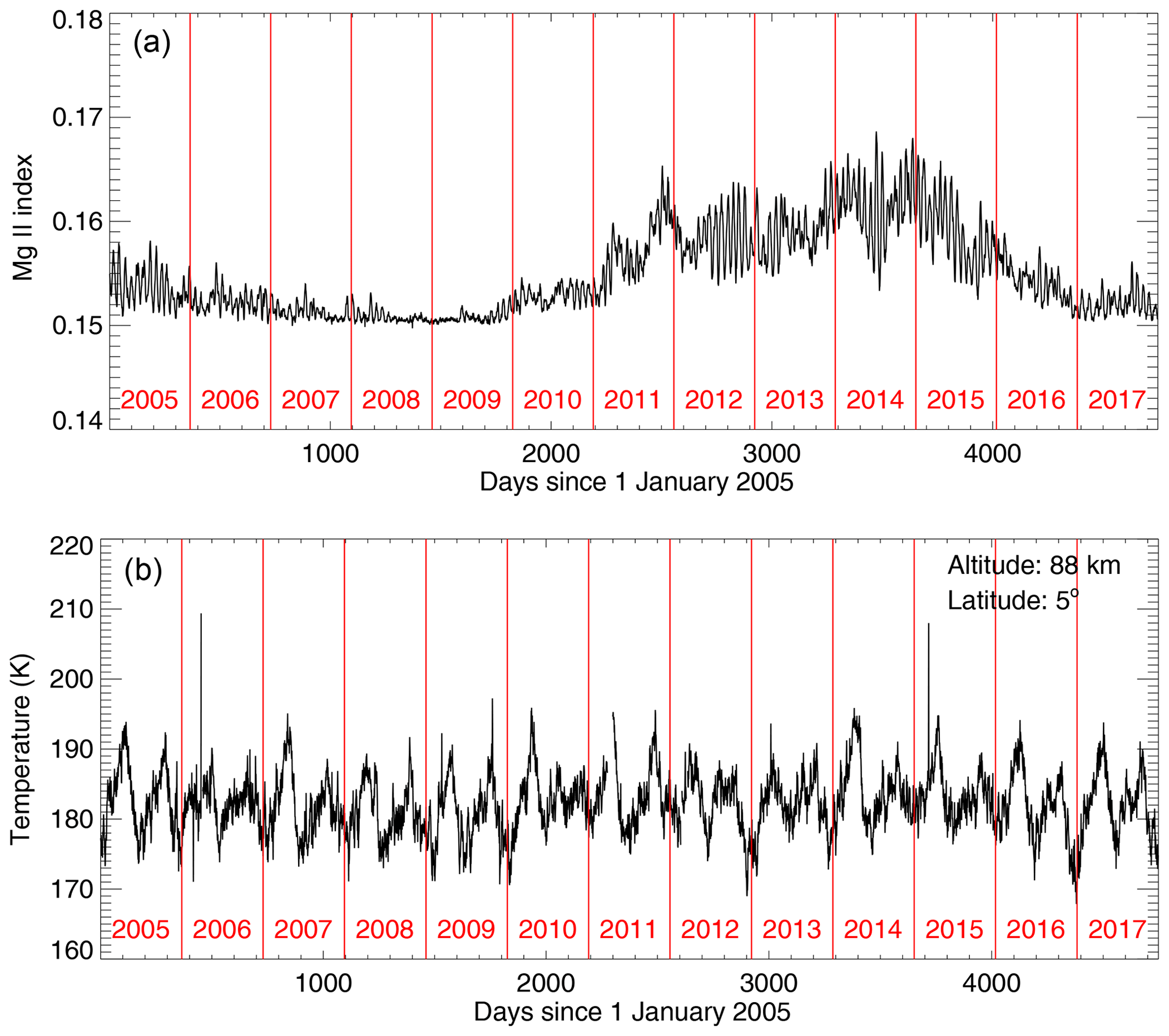
Figure 1 (a) Mg II index data from 2005 to 2017. (b) Time series of zonally and daily averaged temperature for the 5^∘ N (i.e., 0–10^∘ N) latitude bin at 88 km derived from MLS on Aura. Data gaps occur on the days 453–458, 555, 2276–2298, 2605–2609 and 2630–2635.

2.2 MLS on Aura

The National Aeronautics and Space Administration (NASA) Earth observation satellite Aura has been in a near-polar 705 km altitude orbit since 2004. The Microwave Limb Sounder (MLS) on Aura consists of seven radiometers observing emission in the 118 GHz, 190 GHz, 240 GHz, 640 GHz and 2.5 THz regions. The MLS measurements provide vertical profiles of temperature, geopotential height, several atmospheric trace species and ice water content of clouds with near-global coverage on a daily basis (Waters et al., 2006; Livesey et al., 2018).

MLS temperature is retrieved primarily from MLS measurements of the thermal emission of O₂ near 118 and 240 GHz (Schwartz et al., 2008). The isotopic 240 GHz line is the primary source of temperature information in the troposphere (extending the profile down to about 9 km), while the 118 GHz line is the primary source of temperature information in the stratosphere and above (from 90 km down to about 16 km) (Livesey et al., 2018).

In this work, we use the MLS Level 2 temperature product version 4.2. MLS temperature is available from 2 August 2004 to present. The precision and accuracy of the MLS temperature data product are shown in Table 3.22.1 of Livesey et al. (2018). The precision is 1 K or better in the troposphere and lower stratosphere (from 261 to 3.16 hPa), degrading to 3.6 K in the upper mesosphere (at 0.001 hPa). The observed biases based upon comparisons with analyses and other previously validated satellite-based measurements range from −2.5 to +1 K in the troposphere and lower stratosphere, increasing to −9 K at the highest altitude. The recommended useful vertical range for scientific studies is between 261 hPa (10 km) and 0.001 hPa (96 km), and the vertical resolution varies between 3.6 km (at 31.6 hPa) and 13–14 km (at 0.001 hPa). The horizontal resolution is ∼165 km between 261 hPa and 0.1 hPa and degrades to 280 km at 0.001 hPa. To investigate the presence of a 27 d solar cycle signature in the temperature data set and to keep the annual data complete, the period from 1 January 2005 to 31 December 2017 was selected as shown in Fig. 1b. In the following analysis, we first employ the daily and nightly averaged MLS temperature data. In Sect. 4.1.1 and 4.2.1 we investigate how the results change if daytime (or nighttime) measurements only are employed for the analysis.

3 Methodology

The approach employed to analyze the 27 d solar cycle signal in temperature is illustrated in Fig. 2. First, temperature and Mg II index anomalies are calculated (see Sect. 3.1). Next, the SEA method is applied to the temperature and Mg II index anomalies to obtain the epoch-averaged temperature and Mg II index anomalies (Sect. 3.2). Then, the epoch-averaged temperature and Mg II index anomalies are used to perform the sensitivity analysis (Sect. 3.3) and the significance test (Sect. 3.4). The individual steps are described in detail in the corresponding subsections.

Figure 2 Flow chart of the analysis procedure and the input and output parameters.

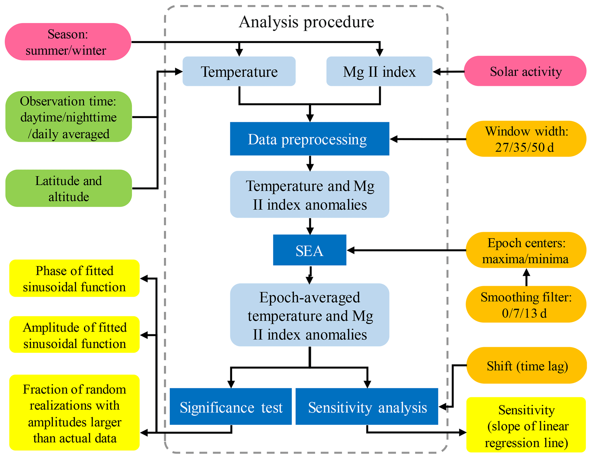
In the process, different input observational and statistical parameters may affect the results. For example, the results may depend on whether daytime, nighttime or daily averaged MLS temperature data are used for the analysis. Other parameters that may affect the results are latitude and altitude, the width of the window used in the data preprocessing, the choice of the epoch centers (maxima or minima of Mg II index anomalies) applied for the SEA, and the smoothing filter used to choose the maxima or minima as epoch centers. In addition, the dependence of the results on solar activity and season also needs to be discussed. To check how these parameters affect the results, different tests are performed and described in Sect. 4.

3.1 Data preprocessing

We defined a standard altitude grid with 36 levels from 20 to 90 km with a step size of 2 km and a standard latitude grid with 18 bins from 90^∘ S to 90^∘ N with a step size of 10^∘. MLS geopotential height was converted to geometric height using the height- and latitude-dependent formula provided by Roedel and Wagner (2011). The temperature data were averaged daily and zonally for each altitude and latitude bin between 1 January 2005 and 31 December 2017.

Figure 1b shows the daily averaged temperature data for an altitude of 88 km and a latitude of 5^∘ N (averaged zonally and over the 0–10^∘ N latitude range). There are five data gaps and six abnormal peaks. The data gaps occur in the following periods: days 453–458 (6 d gap in 2006), day 555 (1 d gap in 2006), days 2276–2298 (23 d gap in 2011), days 2605–2609 (5 d gap in 2012) and days 2630–2635 (6 d gap in 2012). Days are counted starting with 1 January 2005. These gaps exist in the observations at all latitudes and altitudes (see Fig. 3). The white lines in Fig. 3 indicate that temperature data are missing. The outliers/abnormal peaks visible in Fig. 1b occur on days 341, 417, 452, 1532, 1759 and 3717. Note that the outliers appear on different days for different altitudes and latitudes. In order to investigate the presence of a 27 d solar cycle signature in the temperature data set, it is necessary to avoid the invalid points (temperature gaps and outliers) in the SEA. This can be easily implemented in the SEA by ignoring the data gaps and outliers in the averaging procedure (see below).

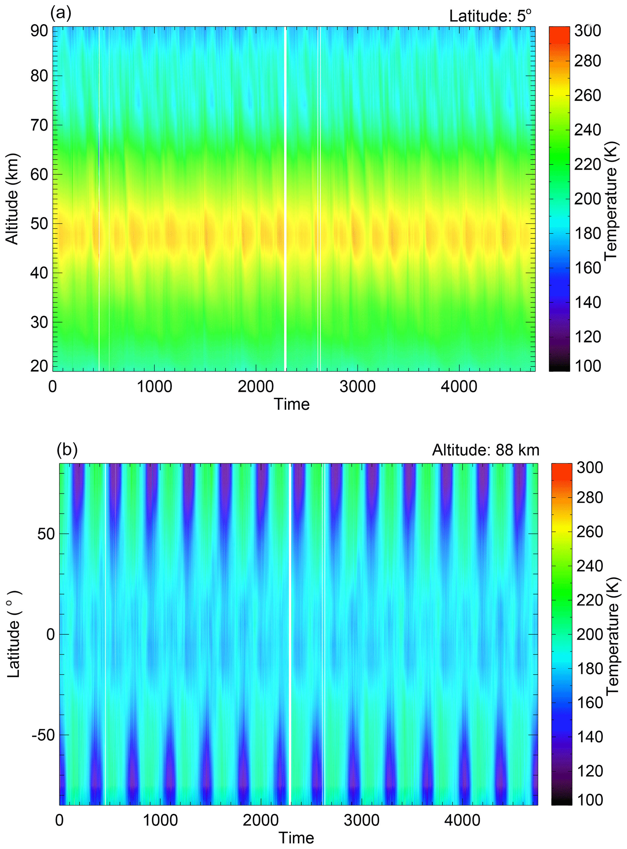
Figure 3 (a) The MLS temperature as a function of altitude and time day at 5^∘ N. (b) The MLS temperature as a function of latitude and time at 88 km altitude. The white lines indicate data gaps.

Next, we apply a 35 d running mean and then calculate the anomalies as the deviation from the running mean for MLS temperature and the Mg II index time series. The resulting temperature anomalies for an altitude of 88 km and a latitude of 5^∘ N are shown in Fig. 4a. We define outliers as data points for which the magnitude of the temperature anomaly exceeds 4 times the standard deviation of the anomaly time series. Figure 4b shows the temperature anomaly with removed outliers. The width of the smoothing window is chosen as 35 d to remove the seasonal modulation of the temperature signal while leaving the variation at shorter timescales unaltered. In Sect. 4.1.1 and 4.2.1 we investigate how the results change if different window widths (e.g., 27 and 50 d) are employed for the analysis. Those steps above are a preparation for the subsequent SEA, significance testing and sensitivity analysis.

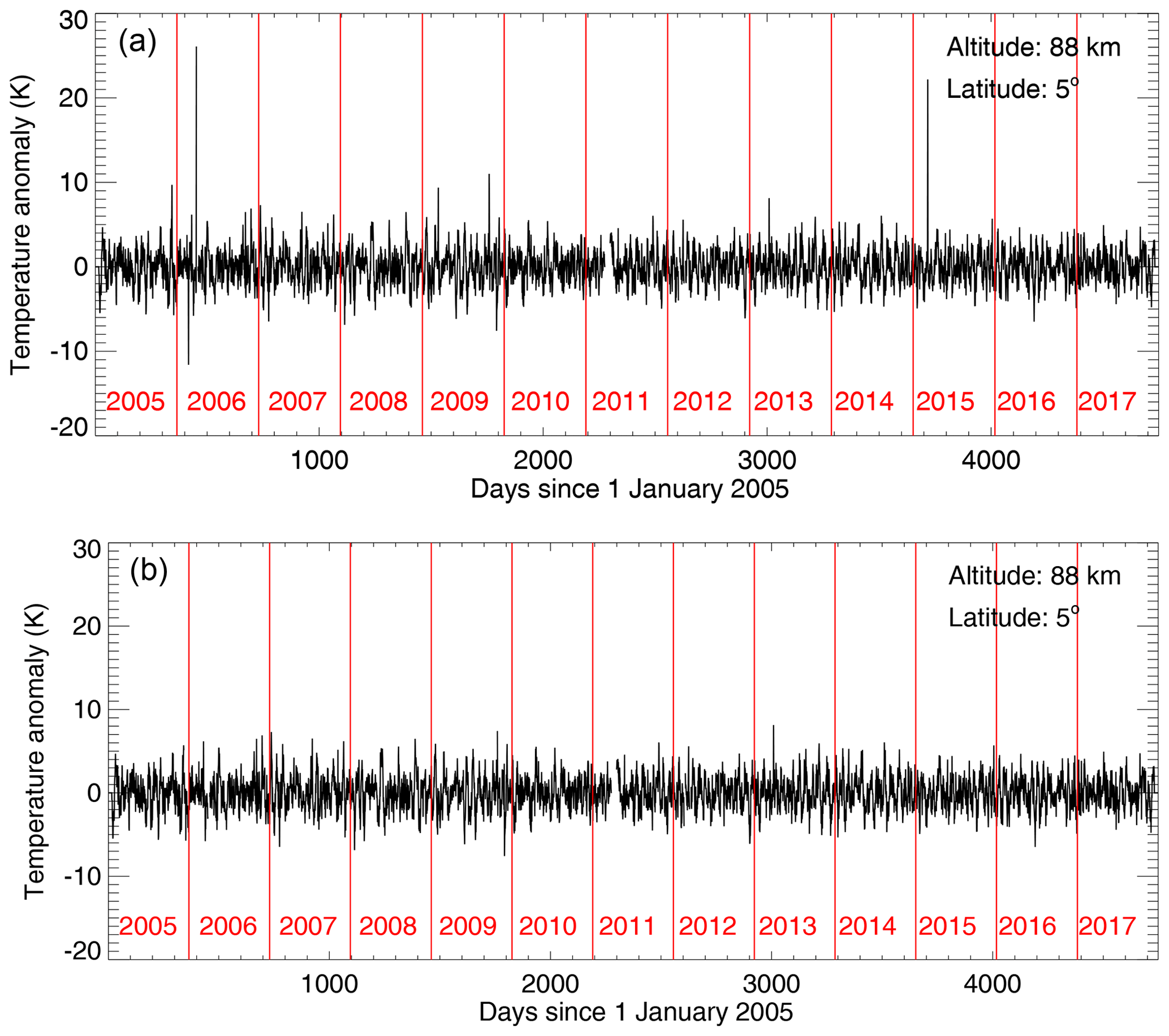
Figure 4 (a) The MLS temperature anomalies generated by subtracting a 35 d running mean from the time series for an altitude of 88 km and a latitude of 5^∘ N. (b) Similar to (a) except for avoiding the abnormal peaks on the days 341, 417, 452, 1532, 1759 and 3717. The plots are based on daily averaged temperature data.

3.2 Superposed epoch analysis (SEA)

To identify weak 27 d solar signatures in temperature time series affected by variability from various sources, the superposed epoch analysis method (SEA) (e.g., Howard, 1833; Chree, 1912) is an effective choice. The SEA is applied to the time series covering the period from January 2005 to December 2017.

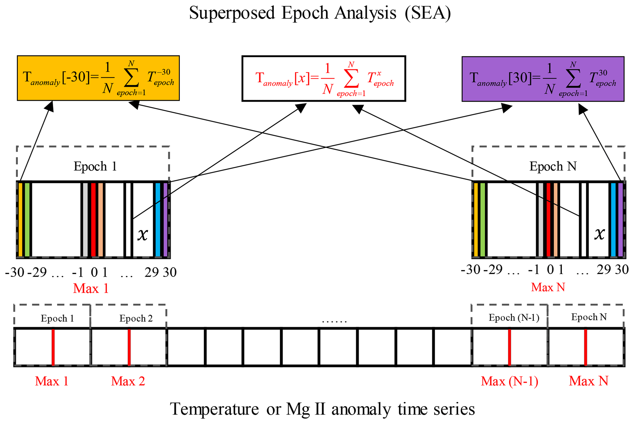
Figure 5 Overview of the superposed epoch analysis (SEA). It should be noted that the epochs are allowed to overlap even though we do not show it in the figure.

An overview of the SEA is shown in Fig. 5. First, the epoch centers need to be chosen. The local maxima in the Mg II index time series – reflecting maxima in solar spectral irradiance – can be used as the epoch centers (represented as Max 1 to Max N in Fig. 5). The Mg II index maxima are identified in the un-smoothed (0 d) or 7 or 13 d smoothed Mg II index anomalies as shown in Fig. 6. The red, blue and green points represent the local maxima identified for the 0, 7 and 13 d smoothed Mg II index anomalies, respectively. We discuss the impact of the smoothing filter on the results in Sect. 4.1.1 and 4.2.1. A similar method can be applied to choose the minima in the Mg II index times series, and we compare the variation in the results by utilizing the maxima or minima of Mg II index anomalies for the SEA in Sect. 4.1.1 and 4.2.1.

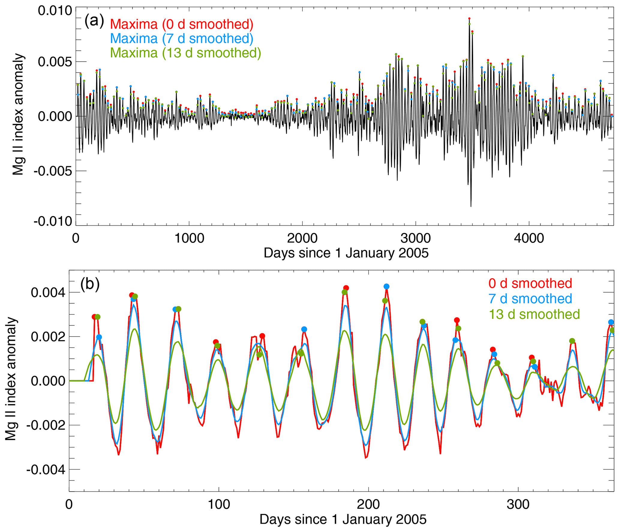
Figure 6 (a) Mg II index anomalies generated by subtracting a 35 d running mean from the time series. The black line presents the un-smoothed or 0 d smoothed Mg II index anomaly. The red, blue and green points are the local maxima chosen from the 0, 7 and 13 d smoothed Mg II index anomalies, respectively. (b) Similar to (a) except for the year 2005 only. In addition, the red, blue and green lines present the Mg II index anomalies smoothed by a 0, 7 and 13 d running mean, respectively.

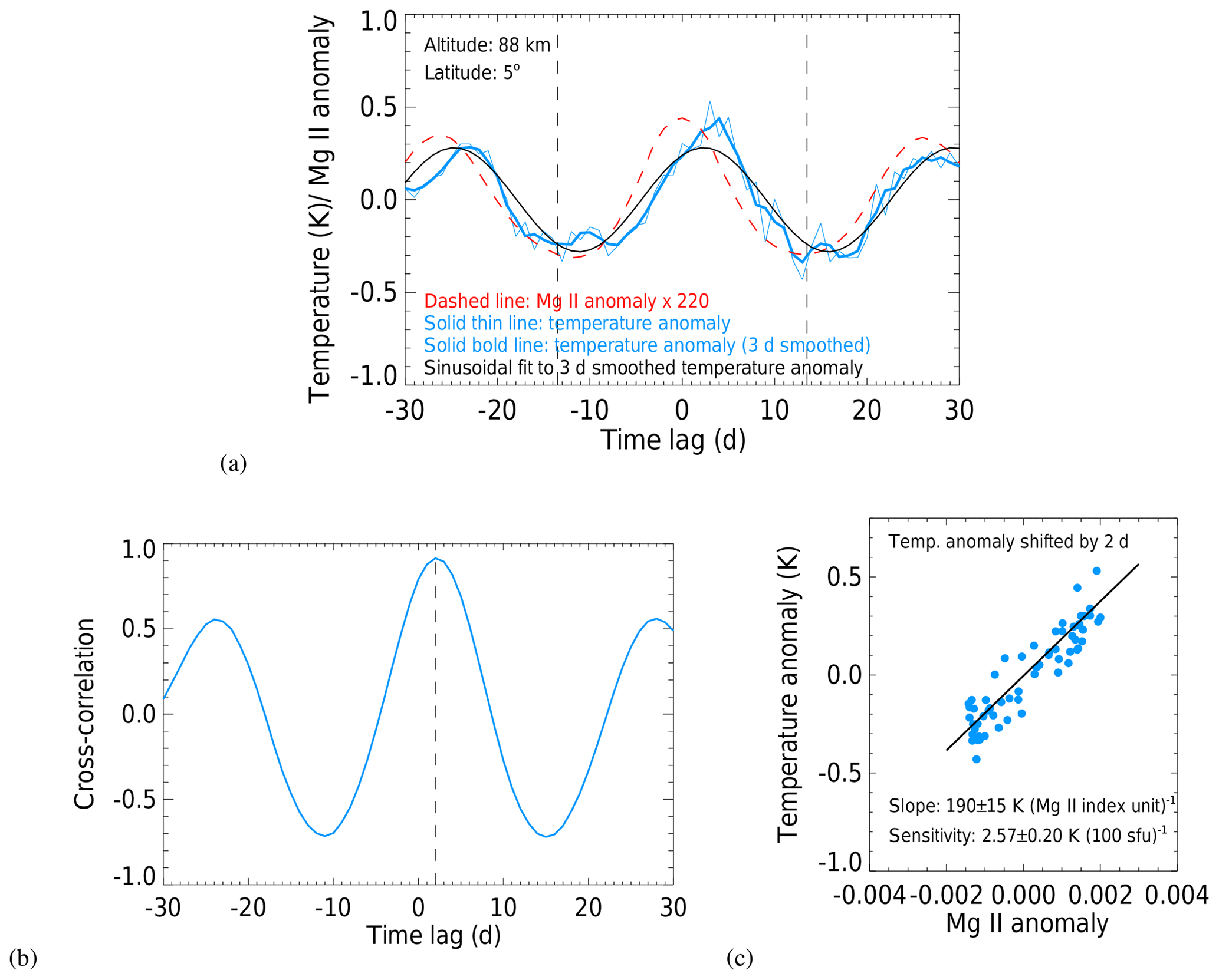
Figure 7 (a) Epoch-averaged Mg II index and temperature anomalies for a total of 173 epochs. The dashed red line is the epoch-averaged Mg II index anomaly multiplied by a factor of 220. The solid thin blue line corresponds to the epoch-averaged temperature anomaly. The solid bold blue line represents the temperature anomaly smoothed with a 3 d running mean. The black line is a sinusoidal fit to the 3 d smoothed epoch-averaged temperature anomaly, with an amplitude of 0.28 K. (b) Cross correlation between the 61 d epoch-averaged temperature and Mg II index anomaly time series (the results correspond to the 35 d running mean) for the time lag between −30 and +30 d. (c) Scatter plot of the 2 d lagged temperature and Mg II index anomalies based on the epoch averages displayed in (a). The black line represents the fitted linear regression line.

Second, we choose 61 d centered at these solar maxima dates as an analysis epoch (i.e., 30 d before and after these maxima). The whole time series from 1 January 2015 to 31 December 2017 will be divided into N epochs, and each epoch covers 61 d. Finally, the epoch-averaged temperature anomaly (T_anomaly[x]) is obtained by averaging N temperatures ($T_{\mathrm{epoch}}^x$) of the corresponding day (x) in each 61 d epoch, see Eq. (1).

$$\begin{array}{}\text{(1)}& T_{\mathrm{anomaly}}\left[x\right]={\displaystyle \frac{\mathrm{1}}{N}}\sum _{\mathrm{epoch}=\mathrm{1}}^N{T}_{\mathrm{epoch}}^x\end{array}$$

Here, x represents an integer between −30 and 30. Similarly, the epoch-averaged Mg II anomaly is determined this way. Figure 7a displays an example of the resulting epoch-averaged temperature (at 88 km and 5^∘ N) and Mg II index anomalies. The Mg II index anomaly exhibits very symmetric behavior with a maximum at zero day time lag and minima near ±13 d, as expected. The epoch-averaged temperature anomaly also shows a clear maximum but with a time lag of 2 d, indicating that the response in mesospheric temperature to the solar forcing occurs with a time lag. The obtained epoch-averaged temperature and Mg II index anomalies (un-smoothed) are used in the sensitivity analysis. A 3 d smoothing is applied to epoch-averaged temperature and Mg II index anomalies for the significance test.

3.3 Sensitivity analysis

The resulting epoch-averaged temperature and Mg II index anomalies are used to determine the sensitivity of middle atmospheric temperature to changes in the solar activity represented here by the Mg II index. The relationship between temperature anomaly (T_anomaly[x]) and Mg II index anomaly (Mg II_anomaly[x]) can be represented by a linear regression line (see Eq. 2) if the maxima in the epoch-averaged anomalies occur at the same time lag. The sensitivity is directly determined by the slope (k) of a linear regression line to the data points, i.e., un-smoothed epoch-averaged temperature and Mg II index anomalies.

$$\begin{array}{}\text{(2)}& T_{\mathrm{anomaly}}\left[x\right]=b+k\times \mathrm{Mg}{\mathrm{II}}_{\mathrm{anomaly}}\left[x\right]\end{array}$$

However, as shown in Fig. 7a, there is a time lag or shift (l) between solar maximum and temperature maximum. If the times of the maxima do not coincide, then an ellipse is fitted instead of a straight line. To remove the phase shift between the two anomalies, we need to shift the temperature curve by l d to obtain the time-lagged epoch-averaged temperature anomalies T_anomaly[x+l]. Then the sensitivity parameter (k) is derived from Eq. (3).

$$\begin{array}{}\text{(3)}& T_{\mathrm{anomaly}}[x+l]=b+k\times \mathrm{Mg}{\mathrm{II}}_{\mathrm{anomaly}}\left[x\right]\end{array}$$

The phase lag (l) can be determined by time-lagged cross-correlation as shown in Fig. 7b. The sensitivity for this particular combination of altitude and latitude is obtained by shifting the epoch-averaged temperature anomaly backwards by 2 d, i.e., $l=-\mathrm{2}$, see Fig. 7c. The sensitivity obtained for a 35 d window width, a 7 d smoothing filter and using maxima of the Mg II index anomaly as the epoch centers is 190 (±15) K per (Mg II index unit). The relationship between the Mg II index and the F10.7 cm radio flux was established by a linear regression to annually averaged values for the years 2003 to 2010 – ΔMgII ∕ ΔF10.7 = 0.0135 Mg II index unit (100 sfu)⁻¹ – and the sensitivity value translates to 2.57 (±0.20) K (100 sfu)⁻¹. The result is in very good agreement with the conclusion of von Savigny et al. (2012). They analyzed zonally averaged OH(3–1) rotational temperatures at 87 km for the [0, 20^∘ N] latitude range using the Mg II index derived from SCIAMACHY and found a temperature sensitivity to solar forcing in terms of the 27 d solar cycle of 182 (±69) K per (Mg II index unit) or 2.46 (±0.93) K (100 sfu)⁻¹. We need to point out, however, that von Savigny et al. (2012) analyzed a much more limited time period – i.e., from April 2005 to October 2006 – compared to the results presented here. More comparisons of our sensitivity results to previously published ones are presented in Sect. 4.2.2 and 4.2.3.

3.4 Significance testing

We use a similar Monte Carlo test method as is used in von Savigny et al. (2019) to examine the significance of the obtained results. Instead of using local solar maxima as the epoch centers in the SEA, the epoch centers are chosen randomly, and the SEA is repeated. The number of random epochs is the same as in the actual SEA. This procedure is carried out 1000 times. Then a sinusoidal function is used to fit every single random realization of the 3 d smoothed epoch-averaged temperature anomaly. Comparing the amplitude of the fitted sinusoidal function of the 1000 random cases to the amplitude of the actual case, the statistical significance of the SEA results can be evaluated. The amplitude and phase of fitted sinusoidal functions, as well as the fraction of random realizations with amplitudes larger than actual data are the results of the significance test. If the fraction of random realizations with amplitudes larger than the amplitude of the actual SEA is close to zero, then the 27 d signature in MLS temperature data is likely not a spurious signature. Figure 8 shows the results of the Monte Carlo significance test at 88 km and 5^∘ N. The local solar maxima used here are determined based on the 7 d smoothed Mg II index anomalies, which were obtained by subtracting a 35 d running mean from the daily Mg II index data.

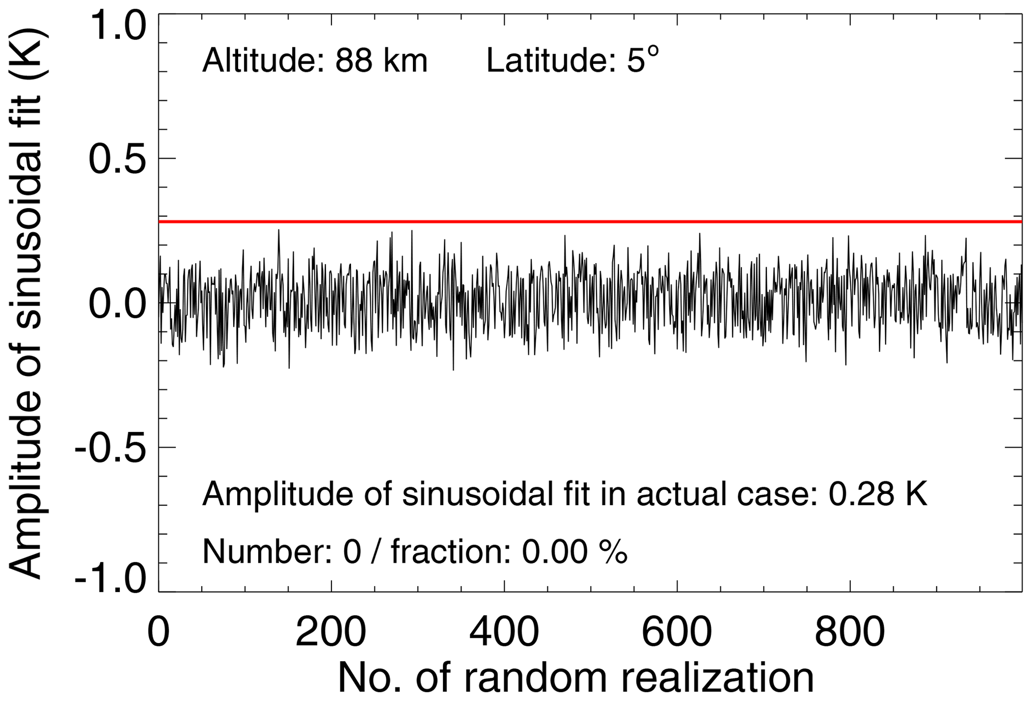
Figure 8 Illustration of the Monte Carlo significance test for an altitude of 88 km and a latitude of 5^∘ N. The red line shows the amplitude of a sinusoidal fit to the extracted 27 d signatures in MLS daily averaged temperature. The black line shows the fitted amplitudes to epoch-averaged temperature anomalies for 1000 randomly chosen epoch ensembles.

4 Results and discussion

The main purpose of the present work is to investigate the presence and characteristics of 27 d solar signatures in the middle atmosphere temperature observed by MLS. In order to investigate how robust the results are, different tests were performed, i.e., a significance test, a sensitivity test, and an investigation of the dependence of the results on real geophysical parameters (i.e., solar activity, season, latitude and altitude) and on statistical/numerical parameters (i.e., window width, epoch centers and smoothing filter).

4.1 Significance test results

The significance testing method was described in Sect. 3.4. To investigate the dependence of the significance results on altitude and latitude, the width of the window, epoch centers and the temperature observations, these tests were performed at each altitude and latitude, for different window widths of 27, 35 and 50 d, as well as different local maxima chosen by 0 or 7 or 13 d smoothed Mg II index anomalies, for daytime, nighttime and daily averaged temperature observations.

4.1.1 Dependence of the results on statistical parameters

The dependence of the results on the different parameters is carried out based upon temperature data in the tropical (5^∘ N) mesopause region (88 km). Table 1 lists the results for the different statistical parameters considered and for the different observational temperature (daytime, nighttime and daily averaged temperature) data sets. The maximum and minimum of the fraction of random realizations with amplitudes larger than actual data are underlined. The max-to-min variation in the fraction for the daytime temperature case is larger than the one for the nighttime and daily averaged temperature cases. In terms of daily averaged temperature, the maximum and minimum fractions are about 1.0 % and 0.0 %, respectively. That is, the variation in the fraction is about 1.0 % for different input parameters. For nighttime temperature, the maximum and minimum fractions are about 1.9 % and 0.0 %, respectively. The max-to-min variation in the fraction is about 1.9 %, but for the daytime temperature, the maximum and minimum fractions are about 28.6 % and 1.5 %, respectively. The max-to-min variation in the fraction increases to about 27.1 %. The exact origin of this different behavior of the daytime temperature data is currently unknown. More discussion on the dependence of the results on statistical parameters at different latitudes and altitudes will be given in Sect. 4.1.2.

Table 1 Significance testing results for different input parameters used in the analysis. The temperature data at a latitude of 5^∘ N and altitude of 88 km are used here. There are two parameters shown in the table. The first one is absolute amplitude in K of the fitted sinusoidal function. The second one is the fraction (%) of random realizations with amplitudes larger than actual data. The values in bold font correspond to the maximum and minimum of the fraction of random realizations with amplitudes larger than the actual data for the daily averaged, the daytime and the nighttime measurements.

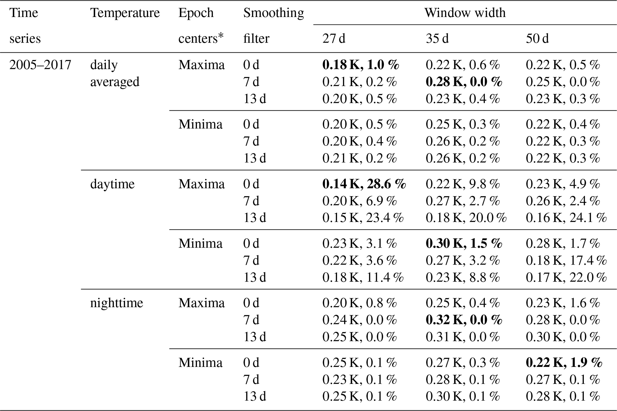
^∗ Maxima/minima of Mg II index anomaly.

4.1.2 Dependence of the results on latitude

We performed the significance test for the daily averaged temperature from 2005 to 2017 for the latitude range from 85^∘ S to 85^∘ N and the altitude range from 20 to 90 km. The resulting fraction of random realizations with amplitudes larger than the actual SEA is displayed in Fig. 9 as a function of latitude and altitude. For the results shown in Fig. 9a, the local solar maxima used in the SEA are chosen from the 7 d smoothed Mg II index anomalies obtained by subtracting a 35 d running mean from the Mg II index data. The temperature anomalies used in the SEA are obtained by subtracting a 35 d running mean from the daily averaged temperature time series. As shown in the figure, there exists a complex pattern of latitude/altitude regions with low fractions indicating that the identified 27 d signatures are most likely not caused spuriously – making a solar origin likely. As shown in the figure, fractions of less than 10 % (high significance) appear in the tropics for the altitude range of 40–60 and 80–90 km, as well as at 40^∘ N for the altitude of about 65 km. The high significance also appears at the high latitudes, e.g., at 70–85^∘ S for the altitude ranges of 30–40 and 60–80 km and at 80–85^∘ N for altitudes of around 40 km.

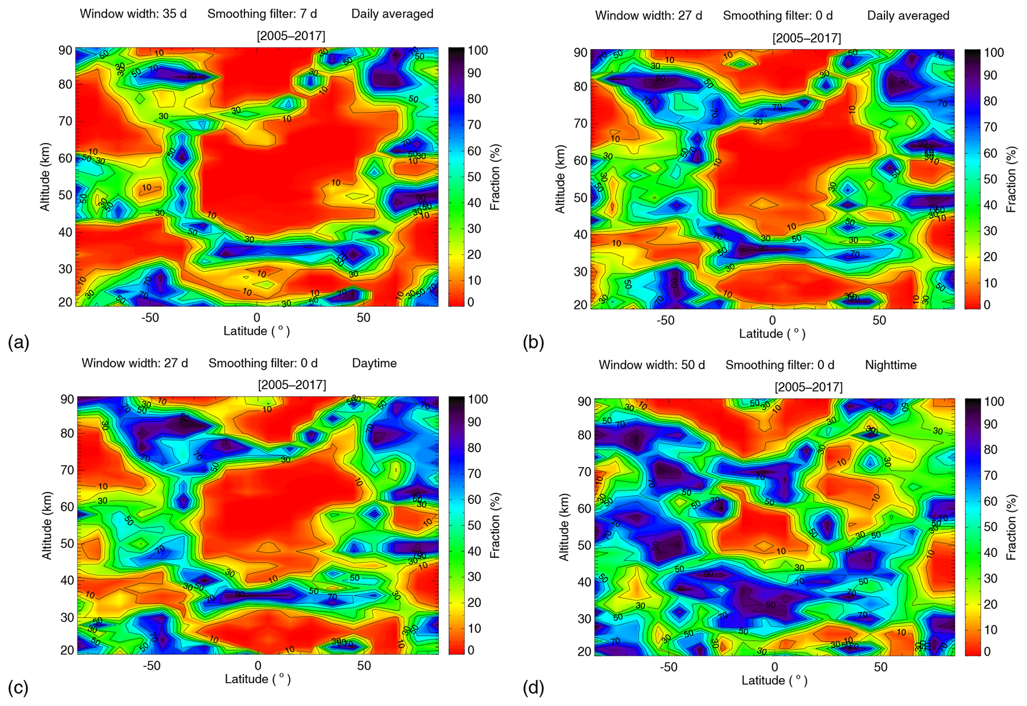
Figure 9 (a) The fraction of random realizations with amplitudes larger than the actual SEA based on the daily averaged temperature data for latitudes ranging from 85^∘ S to 85^∘ N and altitudes ranging from 20 to 90 km. A 35 d window width, 7 d smoothing filter and maxima of the Mg II index anomaly are used in this test. (b) Similar to (a) except that a 27 d window width and 0 d smoothing filter are used. (c) Similar to (a) except that a 27 d window width, 0 d smoothing filter and daytime temperature data are used. (d) Similar to (a) except that a 50 d window width, 0 d smoothing filter, nighttime temperature data and minima of the Mg II index anomaly are used.

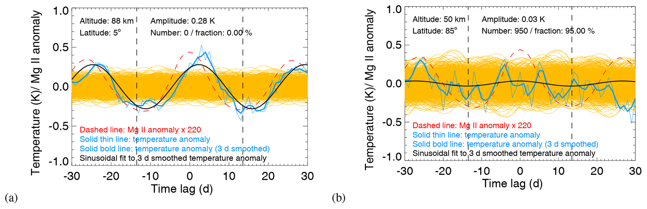
Figure 10 Similar to Fig. 7a except that the orange lines are a sinusoidal fit to the 3 d smoothed epoch-averaged temperature anomalies for 1000 randomly chosen epoch ensembles. (a) For an altitude of 88 km and a latitude of 5^∘ N. (b) For an altitude of 50 km and a latitude of 85^∘ N.

In addition, Fig. 10 provides two examples of high- and low-significance cases. Figure 10a shows the epoch-averaged Mg II index and temperature anomalies and the sinusoidal fit to the 3 d smoothed epoch-averaged temperature anomalies for the actual SEA and for 1000 randomly chosen epoch ensembles at 88 km for a latitude of 5^∘ N. There is no random sinusoidal fit amplitude larger than the actual one, that is, the fraction of the significance test is 0.0 %. Figure 10b is a significance test result for an altitude of 50 km and a latitude of 85^∘ N. In this case 95.0 % of the random sinusoidal fit amplitudes are larger than the amplitude of the actual analysis.

In order to check the influence of the input parameters on the results at different latitudes, we show in Fig. 9 the significance results for some of the combinations of input parameters yielding the largest fractions of random realizations with amplitudes larger than the actual SEA (see Table 1). The results obtained using a 27 d window width and 0 d smoothing filter are shown in Fig. 9b. The results obtained using a 27 d window width, a 0 d smoothing filter and daytime temperature data are shown in Fig. 9c. The results obtained using a 50 d window width, a 0 d smoothing filter, nighttime temperature data and minima of Mg II index anomaly are shown in Fig. 9d. The regions of high significance obviously become smaller in Fig. 9b–d, but the locations of these regions have not changed. That means different input parameters have an impact on the results but will not affect the overall characteristics.

4.1.3 Dependence of the results on season

To determine whether the 27 d solar cycle signal in middle atmospheric temperature depends on season, the SEA and the subsequent significance tests were performed for winter and summer separately. We assume that “winter” includes the 6 months of October, November, December, January, February and March, and “summer” includes the other 6 months for the Northern Hemisphere. For the Southern Hemisphere, it is the opposite. More than three months for each season are considered here in order to increase the number of epochs available for analysis.

Figure 11 (a–b) Similar to Fig. 9a, except for different seasons. (c–f) Sensitivity and shift for latitudes from 85^∘ S to 85^∘ N and altitudes from 20 to 90 km for different seasons. Panels (a), (c) and (e) are the results for the time range from October to March (northern winter/southern summer), and panels (b), (d) and (f) are the results for the time range from April to September (northern summer/southern winter).

The significance testing results depending on season are shown in Fig. 11a–b. The input parameters used in this analysis are the same as in Fig. 9a. In the Southern Hemisphere, the 27 d solar cycle signal in daily averaged temperature is more obvious in winter than in summer. In the Northern Hemisphere, the 27 d signature in temperature at low latitudes (below 50^∘) for the altitude of 35–60 km is more significant in summer than in winter, but for the altitude of 20–30 km the signature is more significant in winter. At high latitudes (70–85^∘ N), the 27 d signature is more significant in winter than in summer, especially for the middle stratosphere (30–40 km). In total, the region of high significance is larger for “summer” months (October–March) than “winter” months (April–September) for the global region.

An important finding is that large differences exist between Northern Hemisphere winter and summer. For northern summer (see Fig. 11b), the latitude–altitude ranges with fractions less than 10 % – indicative of a likely solar origin of the identified signatures – are significantly larger than for northern winter (see Fig. 11a). These differences could be related to enhanced planetary wave activity during Northern Hemisphere winter, leading to enhanced overall atmospheric variability and consequently making the identification of a 27 d solar signature in atmospheric temperature more difficult.

4.1.4 Dependence of the results on solar activity

In addition, we investigated the dependence of the results on solar activity. The comparison of the strong solar activity years (2011–2014) with the weak solar activity years (2007–2009) is shown in Fig. 12a–b. The input parameters used here are identical with the ones for Fig. 9a. The region of high significance is larger for strong solar activity years than for weak solar activity years. For weak solar activity years, the region of high significance mainly concentrates in the equatorial mesopause region as shown in Fig. 12b. For strong solar activity years, the region of high significance is more distributed over high latitudes, mainly at 70–85^∘ N and 40–60^∘ S at around 40 km and at 70–85^∘ S at around 60–80 km.

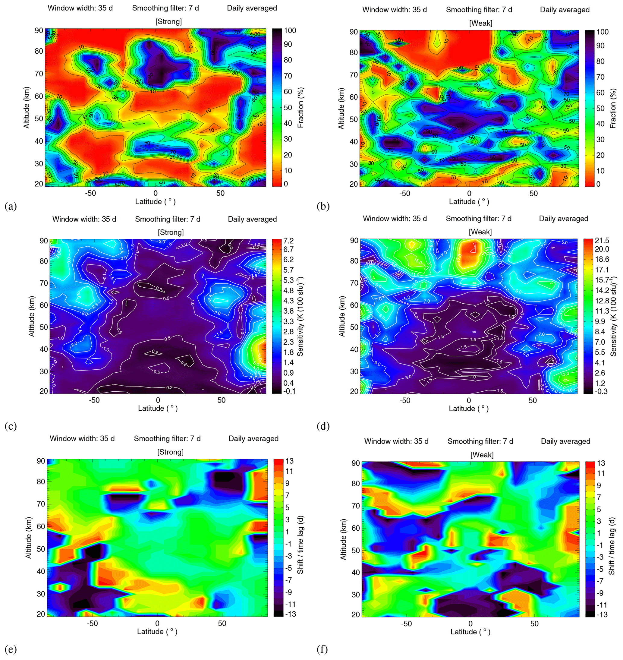
Figure 12 (a–b) Similar to Fig. 9a, except for strong and weak solar activity years. (c–f) Sensitivity and shift for latitudes from 85^∘ S to 85^∘ N and altitudes from 20 to 90 km for different solar activity.

The results demonstrate that the overall significance of the potential 27 d solar signatures in temperature is generally much lower for solar minimum conditions (see Fig. 12b) than for solar maximum conditions (see Fig. 12a). An exception is the tropical mesopause region, where the fraction of random realizations with amplitudes exceeding the amplitude of the actual SEA is smaller for low solar activity than for enhanced solar activity. The reasons for this behavior are currently not understood. The general decrease in the significance with decreasing solar activity is, however, as expected. It is also worth pointing out that the overall significance of the results (as quantified by the latitude–altitude ranges with fractions less than 10 %) is smaller for enhanced solar activity compared to analyzing the entire data set (compare Figs. 12a and 9a). This can be explained by the reduced number of epochs available if only parts of the time series are analyzed and highlights the importance of the length of the time series for obtaining statistically significant results.

4.2 Sensitivity analysis

The temperature sensitivity to solar forcing was calculated with the method described in Sect. 3.3. Similar to the significance testing, we also investigated the dependence of the sensitivity results on different input and observational parameters.

4.2.1 Dependence of the results on statistical parameters

The sensitivity analysis was performed first with the temperature data at the mesopause (88 km) and in the tropics (5^∘ N). Table 2 lists the sensitivity values (i.e., the slope of fitted linear regression line) and the uncertainties depending on the different settings. The underlined values in the table represent the maximum and minimum sensitivity values for different cases. The uncertainties are below 0.6 K (100 sfu)⁻¹. The maximum of the sensitivity is 2.74 (±0.28) K (100 sfu)⁻¹ for daily averaged temperature, 3.18 (±0.40) K (100 sfu)⁻¹ for daytime temperature and 2.95 (±0.45) K (100 sfu)⁻¹ for nighttime temperature. The minimum of the sensitivity is 1.82 (±0.27) K (100 sfu)⁻¹ for daily averaged temperature, 1.33 (±0.34) K (100 sfu)⁻¹ for daytime temperature and 1.81 (±0.38) K (100 sfu)⁻¹ for nighttime temperature. The max-to-min variation in the sensitivity value due to different input parameters is 0.92 K (100 sfu)⁻¹ for daily averaged temperature, 1.85 K (100 sfu)⁻¹ for daytime temperature and 1.14 K (100 sfu)⁻¹ for nighttime temperature. Thus, the influence of the input parameters on the sensitivity result is relatively smaller in daily averaged temperature. This feature is in line with the results derived from the significance test which was discussed in Sect. 4.1.1.

Table 2 Sensitivity (unit: kelvin per 100 solar flux units ) and the uncertainties of different cases at a latitude of 5^∘ N and altitude of 88 km. The sensitivity value is linearly fitted by the time lagged epoch-averaged temperature anomaly with the epoch-averaged Mg II index anomaly. The values in bold font correspond to the maximum and minimum of the sensitivity value for the daily averaged, the daytime and the nighttime measurements.

^∗ Maxima/Minima of Mg II index anomaly.

Overall, there is a tendency toward larger sensitivities if a wider window is used for determining the anomalies. The effect is particularly pronounced for the cases with a 0 and 7 d smoothing of the anomalies. This dependence of the sensitivities on window width may be expected, because, for narrower window widths, parts of the 27 d signatures present may be removed. The same window width is, however, also used for determining the Mg II index anomalies so that part of this effect is compensated, reducing the effect of window width on the sensitivity value. It is also worth pointing out that, for most cases, the sensitivity values for the different window widths agree within combined uncertainties.

4.2.2 Dependence of the results on latitude

Next, we performed the sensitivity analysis for the daily averaged temperature from 2005 to 2017 for latitudes from 85^∘ S to 85^∘ N and altitudes from 20 to 90 km. For this analysis the local solar maxima used in the SEA were determined based on the 7 d smoothed Mg II index anomalies obtained by subtracting a 35 d running mean from the Mg II index data. The temperature anomalies used in the SEA are obtained by subtracting a 35 d running mean from the daily averaged temperature time series. The resulting sensitivity values and shifts (time lag) are displayed in Fig. 13. The obtained sensitivity values range from −0.02 to 5.34 K (100 sfu)⁻¹. There are two distinct features in Fig. 13a. First, the sensitivity generally increases with increasing altitude at low latitudes. Second, the higher sensitivity values appear near the poles. Near the Equator the sensitivity ranges from ∼0 to 2.80 K (100 sfu)⁻¹, but the maximum sensitivity occurs at 85^∘ N for an altitude of about 40 km. In addition, two distinct features are present in the 70–80 km altitude range for southern high latitudes and around 65 km at 40^∘ N.

Figure 13 The (a) sensitivity and (b) shift for all latitudes from 85^∘ S to 85^∘ N and the altitudes from 20 to 90 km, and the analysis year is from 2005 to 2017.

When comparing the graph with the significance test results shown in Fig. 9a, it can be seen that the larger sensitivity values appear in regions with lower fraction, i.e., higher significance, as expected. Figure 13b shows the time lag between local solar maximum (at the 27 d scale) and the temperature maximum. Comparing Fig. 13a with Fig. 13b shows that small time lags tend to occur in latitude–altitude regions with large sensitivity.

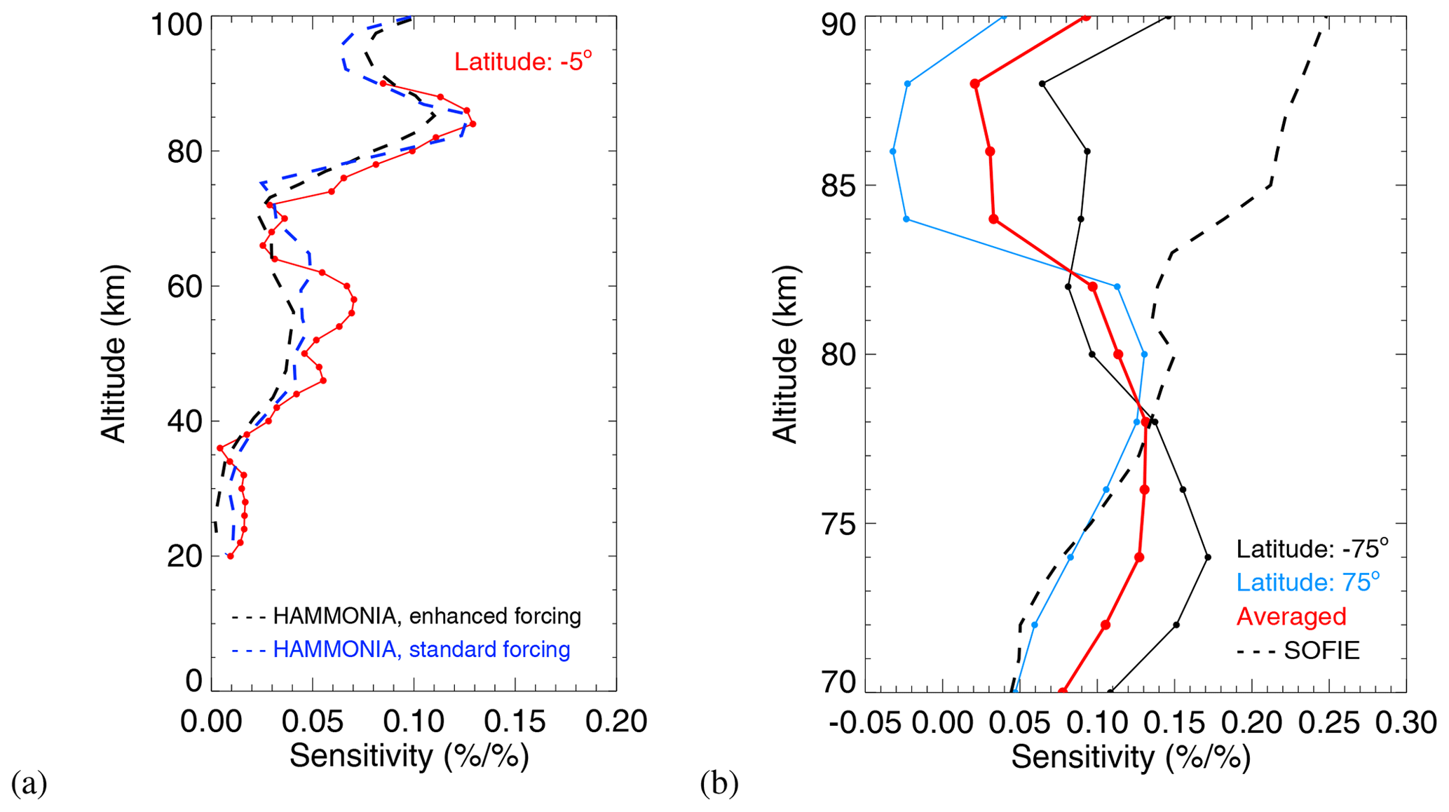
Figure 14 (a) MLS temperature sensitivity profile (red line) (sensitivity expressed as % change in temperature per % change in solar UV flux at 205 nm) for a latitude of 5^∘ S and altitudes ranging from 20 to 90 km for the daily averaged temperature data from 2005 to 2017. The profile is from Fig. 13a. The dashed lines are the sensitivity results from HAMMONIA for enhanced forcing (black) and for standard forcing (blue) calculated by Gruzdev et al. (2009). (b) Similar to (a), except for the southern summer and a latitude of 75^∘ S (solid black line) and for the northern summer and a latitude of 75^∘ N (blue line) for altitudes from 70 to 90 km. The sensitivity profile ( solid black line) is from Fig. 11c. The sensitivity profile (blue) is from Fig. 11d. The red profile is the averaged sensitivities of the black and blue profiles. The dashed black line is the sensitivity results based on SOFIE data from Thomas et al. (2015).

In Fig. 14a we show the MLS temperature sensitivity to 27 d solar forcing as a function of altitude for a latitude of 5^∘ S. In order to compare our results to the model calculations based on the three-dimensional chemistry–climate model HAMMONIA analyzed by Gruzdev et al. (2009) (Fig. 12b of their paper), we converted the sensitivity to % change in temperature per % change in 205 nm solar irradiance. The conversion is based on a linear fit between the Mg II index and the 205 nm solar irradiance measured by the Solar Stellar Irradiance Comparison Experiment (SOLSTICE) on the Solar Radiation and Climate Experiment (SORCE) during the period from 2005 to 2017 (LISIRD, 2019), i.e., ΔMgII $/\mathrm{\Delta }\mathrm{205}=\mathrm{18.928}$ Mg II index unit (W m⁻² nm⁻¹)⁻¹. The percent temperature changes were determined using the mean temperature of 2005–2017 for the latitudes ranging from 85^∘ S to 85^∘ N, and the percent 205 nm irradiance changes were determined using the mean UV 205 nm irradiance between 2005–2017. As shown in Fig. 14a, the maximum is at 84 km and the corresponding sensitivity is 0.13 % per %, a second maximum occurs at 58 km and the corresponding sensitivity is 0.07 % per %. The results are in good agreement with the annually averaged sensitivities for the [20^∘S, 20^∘N] latitude range in Gruzdev et al. (2009) (green lines in Fig. 12b of their paper). Their model results for enhanced forcing show a main maximum at 85 km and a corresponding sensitivity of about 0.11 % per % and a second maximum at 55 km with a sensitivity of about 0.04 % per %, see dashed black line in Fig. 14a. For standard forcing, their model results show a main maximum at 85 km and a corresponding sensitivity of about 0.13 % per %, see dashed blue line in Fig. 14a.

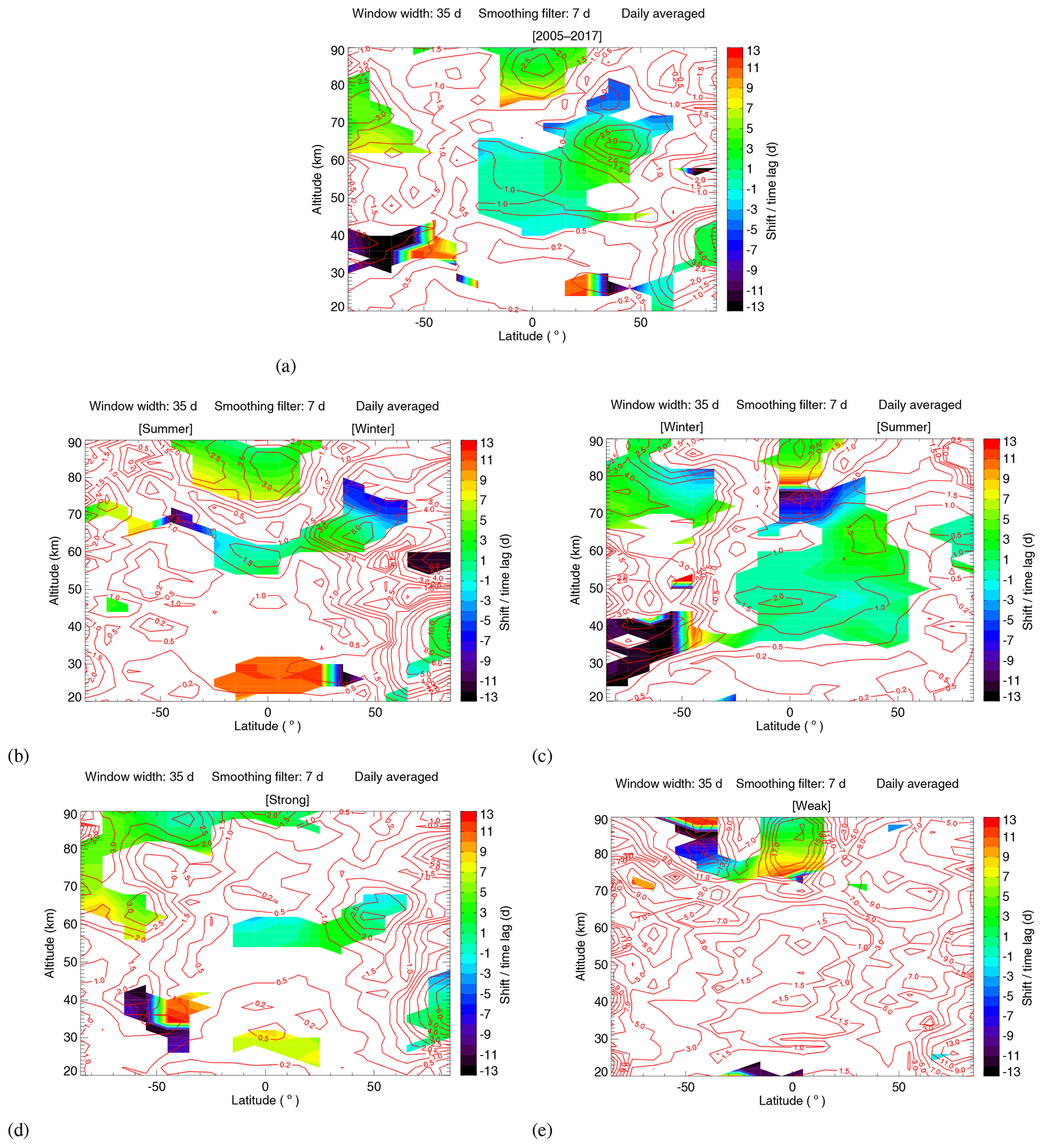
Figure 15 Sensitivity in K (100 sfu)⁻¹ (red contour lines) and shift (color-filled contour) of the region that satisfies the condition that the significance test fraction less is than 10 % for all the latitude from 85^∘ S to 85^∘ N and the altitude from 20 to 90 km for years from 2005 to 2017 (a), for different seasons (b–c) and for different solar activity (d–e).

In order to study the sensitivity features for regions with high significance of the identified 27 d signatures, we choose the region that meets the condition that the significance test fraction is less than 10 %. The white parts in Fig. 15a–e represent the regions with significance test fractions exceeding 10 %. Figure 15a displays the sensitivity and shift of the region of high significance for the latitude range from 85^∘ S to 85^∘ N and the altitude range from 20 to 90 km for years from 2005 to 2017. The red contour lines represent the sensitivity value and the colors represent the shift. The sensitivity is in many cases larger than 1.0 K (100 sfu)⁻¹. The absolute shift is frequently less than 9 d at high altitudes (45–90 km). The shift at low altitudes (20–45 km) varies largely from −13 to +13 d.

4.2.3 Dependence of the results on season

Next, the temperature sensitivity to solar forcing was analyzed for different seasons. Figure 11c–f show the sensitivity and shift for the latitude range from 85^∘ S to 85^∘ N and the altitude range from 20 to 90 km for different seasons. As shown in Fig. 11c–d, the sensitivity in winter is obviously larger than in summer. In the Northern Hemisphere, the maximum sensitivity, i.e., 12.41 K (100 sfu)⁻¹, occurs in winter at 85^∘ N for altitudes of about 40 km. In the Southern Hemisphere, the maximum sensitivity is 5.16 K (100 sfu)⁻¹ and occurs at around 70^∘ S for about 75 km altitude winter. In other words, the sensitivity increases in general with increasing latitude in the winter hemisphere. In summer, the sensitivity shows a tendency to increase with altitude in general. Figure 11e–f show the determined lag. The shifts do not exhibit the same obvious latitude–altitude characteristics as the sensitivity, which is not further investigated here.

The graphs indicate larger sensitivity of atmospheric temperature to solar forcing at the 27 d scale in the winter hemisphere (see Fig. 11c and d) – although one has to keep in mind that the results are not significant at all latitudes and altitudes. The identified interhemispheric difference in temperature sensitivity is in agreement with the model results of Gruzdev et al. (2009), who reported that the temperature response to the 27 d solar cycle at extra-tropical latitudes is seasonally dependent, with frequently higher sensitivities in winter than in summer. This has also been reported, e.g., by Ruzmaikin et al. (2007), who analyzed MLS ozone and temperature observations in the stratosphere. The origin of the enhanced sensitivity in the winter hemisphere – particularly at high latitudes – is not well understood.

In Fig. 14b, we plot the MLS temperature sensitivity profile (% per %) for the southern summer at 75^∘ S (solid black line) and for the northern summer at 75^∘ N (blue line). We used the averaged sensitivity profile (red line) of those two profiles to compare with the results of Thomas et al. (2015) (Fig. 8b of their paper), here represented by dashed black line in Fig. 14b. They analyzed the response of SOFIE temperature observations to the 27 d solar cycle for two Northern Hemisphere summertime seasons (2010, 2011) and three Southern Hemisphere (2011–2012, 2012–2013 and 2013–2014) summertime seasons. At 78 km altitude, our sensitivity is 0.13 % per % which is in excellent agreement with the value reported by Thomas et al. (2015). The MLS temperature sensitivity values reported here are larger than the values derived from SOFIE observations for altitudes below 78 km. Our MLS temperature sensitivity is smaller than the SOFIE-based values for altitudes above 78 km. One possible reason for the differences between MLS and SOFIE results could be the different time periods analyzed in the respective studies. Another reason could be the difference in vertical resolution between MLS (>10 km) and SOFIE (∼2 km) for the range of altitudes relevant here (70–90 km). Also, the spatial and temporal sampling of the MLS and SOFIE measurements differs, as the latitudes of SOFIE solar occultation measurements vary slowly from day to day within the ∼65–85^∘ N and the ∼65–85^∘ S latitude range.

Similar to Sect.4.2.2, we investigate the sensitivity features for the high significance region for different seasons as shown in Fig. 15b–c. The sensitivity is larger than 1.0 K (100 sfu)⁻¹ in most of the high significance region, except for the tropical region at low altitudes (20–30 km) for northern winter and southern summer season. In the Northern Hemisphere, the large shift of ±13 d appears at around 75 km near the Equator in summer, but in winter it occurs at 85^∘ N for an altitude of about 60 km and at 0–45^∘ N for the altitude range 20–30 km. In the Southern Hemisphere, a large shift of ±13 d occurs at low latitudes for the altitude range from 20–30 km in summer, but it is mainly focused at high latitudes for the altitude range from 20 to 45 km in winter.

4.2.4 Dependence of the results on solar activity

Last, we investigated the dependence of the resulting sensitivity on solar activity. The sensitivity values of the strong solar activity years (2011–2014) and the weak solar activity years (2007–2009) are shown in Fig. 12c–d. For strong solar activity years, the sensitivity ranges from −0.06 to 7.20 K (100 sfu)⁻¹. The sensitivity values are larger at high latitudes than at low latitudes. In addition, the maximum appears at 85^∘ N at about 40 km altitude. The sensitivity values of the strong solar activity years are much smaller than the values in the weak solar activity years. However, unusually high values up to 21.48 K (100 sfu)⁻¹ are found for the weak solar activity years, with the maximum occurring at the equatorial mesopause. Such high sensitivities in weak solar activity years likely is an indication that temperature is affected by factors other than the 27 d solar cycle.

Overall, the results show a tendency to enhanced temperature sensitivity to solar forcing during periods of low solar activity. Gruzdev et al. (2009) state that this effect is also present in their model simulations of the effect of the 27 d solar UV forcing on middle atmospheric temperatures, where the sensitivities of temperature to solar activity generally decrease when the forcing increases. For the analysis presented here it is important to remember that, for solar minimum conditions, the 27 d signatures are not statistically significant at most altitudes and latitudes. For this reason the comparison of sensitivity values for periods of high and low solar activity should be interpreted with caution.

Interestingly, increased sensitivity during periods of low solar activity has been reported for 27 d signatures in different atmospheric parameters, including polar summer mesopause temperature (Robert et al., 2010), noctilucent clouds (or polar mesospheric clouds) (Thurairajah et al., 2017) or standard phase heights (von Savigny et al., 2019). These findings may be caused by other sources of variability in a similar period range – likely unrelated to solar forcing – such as planetary wave activity. We refer to von Savigny et al. (2019) for a more detailed discussion on a potential interference by dynamical effects.

Similar to Sect. 4.2.2 and 4.2.3, the sensitivity and shift for the high significance (i.e., fraction <10 %) region for different solar activity are shown in Fig. 15d–e. The colored areas are the latitudes and altitudes that have significant sensitivities. For the 11-year solar maximum, the region of high latitude of 85^∘ N at about 40 km has highly significant sensitivities of about 5.0–7.2 K (100 sfu)⁻¹. For the 11-year solar minimum, the high altitudes of 80–90 km near the Equator have highly significant sensitivities of about 17.0–21.5 K (100 sfu)⁻¹. For strong solar activity years, a large shift of ±13 d occurs at southern extra-tropical latitudes for the altitude range from 25 to 45 km. For weak solar activity years, large shifts of ±13 d occur at southern extra-tropical latitudes for the altitude range from 80 to 90 km and at low latitudes for altitudes around 75 and 20 km.

5 Conclusions

This study reports on the investigation of potential 27 d solar signatures in middle atmospheric temperature. The analysis is based on a 13-year (2005–2017) global temperature data set obtained from spaceborne measurements with the Aura MLS instrument. The results are mainly based on the superposed epoch analysis approach, which is well suited for identifying weak signatures in time series characterized by large variability. The statistical significance of the obtained results was evaluated with a dedicated Monte Carlo approach. On this basis, several new conclusions can be drawn.

1. The analysis showed that a 27 d solar signature in middle atmospheric temperature can be identified with high statistical significance under certain conditions. However, a complex dependence of the significance of the obtained results on several assumptions and parameters was found.

2. The sensitivity of temperature to 27 d solar forcing tends to be larger at high latitudes than at low latitudes.

3. The overall statistical significance of the 27 d signatures is higher for periods of enhanced solar activity than during periods of low solar activity, as expected. The sensitivity analysis showed that even for strong solar activity, the 27 d signatures are not significant at many latitudes and altitudes.

4. Enhanced 27 d signatures during winter time were found. It is noteworthy that the 27 d signatures in both hemispheres have a higher significance for northern summer compared to northern winter, which may be related to enhanced planetary wave activity during Arctic winters.

Several findings indicate the presence of other sources of variability in the 25–30 d period range, likely of a dynamical nature. The separation of these sources – likely unrelated to solar forcing – from a real solar forcing is an intrinsic difficulty when searching for 27 d solar signatures in atmospheric parameters. Further studies on the interference of dynamical effects and/or potential solar impact on these dynamical effects are required for a full understanding of the observed variability in middle atmospheric temperature.