the Creative Commons Attribution 4.0 License.
the Creative Commons Attribution 4.0 License.
 | 10 Feb 2020
On the limit to the accuracy of regional-scale air quality models
Huiying Luo
Marina Astitha
Christian Hogrefe
Valerie Garcia
Rohit Mathur
Regional-scale air pollution models are routinely being used worldwide for research, forecasting air quality, and regulatory purposes. It is well recognized that there are both reducible (systematic) and irreducible (unsystematic) errors in the meteorology–atmospheric-chemistry modeling systems. The inherent (random) uncertainty stems from our inability to properly characterize stochastic variations in atmospheric dynamics and chemistry and from the incommensurability associated with comparisons of the volume-averaged model estimates with point measurements. Because stochastic variations are not being explicitly simulated in the current generation of regional-scale meteorology–air quality models, one should expect to find differences between the model estimates and corresponding observations. This paper presents an observation-based methodology to determine the expected errors from current-generation regional air quality models even when the model design, physics, chemistry, and numerical analysis, as well as its input data, were “perfect”. To this end, the short-term synoptic-scale fluctuations embedded in the daily maximum 8 h ozone time series are separated from the longer-term forcing using a simple recursive moving average filter. The inherent uncertainty attributable to the stochastic nature of the atmosphere is determined based on 30+ years of historical ozone time series data measured at various monitoring sites in the contiguous United States (CONUS). The results reveal that the expected root mean square error (RMSE) at the median and 95th percentile is about 2 and 5 ppb, respectively, even for perfect air quality models driven with perfect input data. Quantitative estimation of the limit to the model's accuracy will help in objectively assessing the current state of the science in regional air pollution models, measuring progress in their evolution, and providing meaningful and firm targets for improvements in their accuracy relative to ambient measurements.
- Article
(2407 KB) - Full-text XML
- BibTeX
- EndNote


Confidence in model estimates of pollutant distributions is established through direct comparisons of modeled concentrations with corresponding observations made at discrete locations for retrospective cases. Pinder et al. (2008) discussed the reducible (i.e., structural and parametric) uncertainties that are attributable to the errors in model input data (e.g., meteorology, emissions, and initial and boundary conditions) as well as our incomplete or inadequate understanding of the relevant atmospheric processes (e.g., chemical transformation, planetary boundary layer evolution, transport and dispersion, deposition, rain, and clouds). Inherent or irreducible (random or unsystematic) uncertainties stem from our inability to properly characterize the stochastic nature of the atmosphere (Wilmott, 1981; Wilmott et al., 1985; Fox, 1984; Rao et al., 1985, 2011a, b; Dennis et al., 2010) and from the incommensurability associated with comparing the volume-averaged model estimates with point measurements (e.g., McNair et al., 1996; Swall and Foley, 2009). Also, without completely knowing the three-dimensional initial physical and chemical state of the atmosphere, its future state cannot be simulated accurately (Lamb, 1984; Lamb and Hati, 1987; Lewellen and Sykes, 1989; Pielke, 1998; Gilliam et al., 2015). Given the presence of the irreducible uncertainties, precise replication of observed concentrations or their changes by the models cannot be expected (Dennis et al., 2010; Rao et al., 2011a; Porter et al., 2015; Astitha et al., 2017).
Whereas an air quality model's prediction represents some time-/space-averaged concentrations, an observation at any given time at a monitoring location reflects an individual event or specific realization out of a population that will almost always differ from the model estimate even if the model and its input data were perfect (Rao et al., 1985). Consequently, comparisons of modeled and observed concentrations paired in space and time indicate biases and errors in simulating absolute levels of pollutant concentrations at individual monitoring sites (Porter et al., 2015). The scientific discussion on modeling uncertainty goes back more than 3 decades with the current practice including data assimilation, ensemble modeling, and model performance evaluation (e.g., Fox, 1981, 1984; Lamb, 1984; Demerjian, 1985; Oreskes et al., 1994; Pielke, 1998; Lewellen and Sykes, 1989; Lee et al., 1997; Carmichael et al., 2008; Hogrefe et al., 2001a, b; Biswas and Rao, 2001; Grell and Baklanov, 2011; Gilliam et al., 2006; Herwehe et al., 2011; Baklanov et al., 2014; Bocquet et al., 2015; Solazzo and Galmarini, 2015a; Ying and Zhang, 2018; McNider and Pour-Biazar, 2020; Stockwell et al., 2020). While ever-improving process knowledge and increasing computational power will continue to help reduce the structural and parametric uncertainties in air quality models, the inherent uncertainty associated with our inability to properly characterize the stochastic nature of the atmosphere will always result in some mismatch between the model results and measurements; this could lead to speculation on the inferred accuracy of the future states simulated by the regional-scale air quality models (Dennis et al., 2010; Rao et al., 2011a; Porter et al., 2015; Astitha et al., 2017; Luo et al., 2019).
The sensitivity of model results to meteorology, chemical mechanisms, and emissions has been examined in numerous studies (e.g., Vautard et al., 2012; Sarwar et al., 2013; Pierce et al., 2010; Napelenok et al., 2011; Kang et al., 2013). Herwehe et al. (2011) attributed the differences in ground-level ozone predictions between the Weather Research and Forecasting (WRF) model coupled with Chemistry (WRF-Chem) and the modeling system consisting of WRF and the Community Multiscale Air Quality (CMAQ) model (WRF-QMAC) to the way meteorology and chemistry interactions are handled within these two modeling systems. Thomas et al. (2019) examined the ozone predictions in the mid-Atlantic region of the United States during June 2016 through a series of simulations with WRF-Chem, focusing on the sensitivity to the meteorological initial/boundary conditions (IC/BCs), emissions inventory (EI), and planetary boundary layer (PBL) scheme. Ying and Zhang (2018) discussed the use of satellite-based observations for improving the predictability of multiscale tropical weather and equatorial waves. Ensemble modeling is being advocated for quantifying the uncertainty in model predictions; however, the spread in the model estimates for the variable of interest reflects the impact of our incomplete or inadequate knowledge of the physical and chemical processes (i.e., the reducible errors stemming from structural and parametric uncertainty) occurring in the atmosphere (Solazzo and Galmarini, 2015b; Thomas et al., 2019; Stockwell et al., 2020). McNider and Pour-Biazar (2020) reviewed the many issues in predicting the prevailing meteorology for regional air quality simulations and indicated that errors in the specification of the physical atmosphere such as temperature, winds, and mixing heights can affect the air quality predictions. Stockwell et al. (2020) discussed the problems relating to the atmospheric chemical mechanisms currently being used for simulating air quality. The current generation of regional models consider only the mean values of a meteorological variable for a given timescale and the average rate constant derived from gas chamber experiments for chemical reactions and does not include their fluctuations in solving the equations of motion for each time step. Further, the current operational regional-scale meteorological and air quality models do not explicitly simulate the stochastic nature of the atmosphere and, as such, typically miss the extreme values at both the low and high ends of the concentration distribution function.
In most applications of regional-scale air quality models, statistical metrics such as bias, the root mean square error (RMSE), correlation, and the index of agreement are used to judge the quality of model predictions and determine if the model is suitable for forecasting or regulatory purposes (e.g., Fox, 1981, 1984; Solazzo et al., 2012; Appel et al., 2012; Simon et al., 2012; Foley et al., 2014; Ryan, 2016; Emery et al., 2016; Zhang et al., 2016; U.S. Environmental Protection Agency, 2018). While significant improvements in the formulation, physical and chemical parameterizations, and numerical techniques have been implemented in atmospheric models over the past 3 decades, it is not clear if the improvement claimed in the model's performance relative to the routine network measurements is statistically significant based on these metrics (Hogrefe et al., 2008). Also, no assessments have been made to date on the errors that are to be expected even from “perfect” regional-scale air quality modeling systems. To estimate such irreducible model errors due to atmospheric stochasticity (which we consider to be the errors that are expected even from a perfect model – devoid of structural and parametric uncertainties – with perfect – error-free – inputs), we analyzed the observed daily maximum 8 h (DM8HR) ozone time series data at monitoring locations across the contiguous United States (CONUS) during the 1981–2014 time period and present the results of this analysis in Sect. 3.1. In Sect. 3.2, we illustrate how this information could be used in guiding model development specifically aimed at addressing reducible errors in the synoptic (SY) component by contrasting the results from Sect. 3.1 with analysis using the synoptic component from a 21-year simulation performed with the fully coupled WRF-CMAQ simulations covering the 1990–2010 period. Since we relied on multi-decadal historical ozone observations to assess the impact of the stochastic nature of the atmosphere, the results presented here are applicable to both forecasting and retrospective applications of current regional-scale air quality models.
Ground-level DM8HR ozone data covering CONUS during May to September in each year were obtained from the U.S. Environmental Protection Agency's (EPA) Air Quality System (AQS) (see https://www.epa.gov/aqs, last access: 3 February 2020). A valid ozone season consists of at least 80 % data coverage during May to September at each station. A total 185 monitoring stations with at least 30 valid years (to provide enough variety of synoptic conditions, denoted hereafter as 30+ in this paper) from the year 1981 to 2014 are analyzed. Also, fully coupled WRF-CMAQ model simulations over CONUS for the 1990–2010 period were utilized in this study to demonstrate a new perspective on model performance evaluation. To ensure better characterization of the prevailing meteorology (i.e., synoptic forcing) in the retrospective 21-year WRF-CMAQ simulations, four-dimensional data assimilation (FDDA) was utilized following the methodology suggested by Gilliam et al. (2012) and modified for fully coupled meteorology–chemistry model applications as described in Hogrefe et al. (2015). The model setup and performance evaluation of these historical multiyear WRF-CMAQ simulations have been published by Xing et al. (2015), Gan et al. (2015), and Astitha et al. (2017). Time-varying chemical lateral boundary conditions are nested from the 108 km hemispheric WRF-CMAQ simulation from 1990 to 2010 (Xing et al., 2015).
It has been shown that time series of the daily maximum 8 h ozone concentrations contain fluctuations operating on different timescales (e.g., intra-day forcing induced by the fast-changing emissions and atmospheric boundary layer evolution; diurnal forcing induced by the day and night differences; and synoptic forcing induced by the passage of weather systems across the country, sub-seasonal forcing due to the Madden–Julian Oscillation – MJO, and long-term forcing induced by emissions, El Niño–Southern Oscillation – ENSO, climate change, and other slow-varying processes such as seasonal and sub-seasonal variations in the atmospheric deposition and stratosphere–troposphere exchange processes) as noted by Rao et al. (1997), Vukovich (1997), Hogrefe et al. (2000), Porter et al. (2015), Astitha et al. (2017), Xing et al. (2016), and Mathur et al. (2017). Variations in the 8 h ozone can be thought of comprising of the baseline (BL) of pollution that is created by various emitting sources and modulated by the prevailing synoptic weather conditions (Rao et al., 1996, 2011b). Thus, the magnitude of the baseline concentration and the strength of the synoptic component should be viewed as the necessary and sufficient conditions for how high ozone levels can reach on a given day (Astitha et al., 2017). Scale separation can be achieved by applying filtering methods such as the empirical mode decomposition (EMD; Huang et al., 1998), elliptic filter (Poularika, 1998), Kolmogorov–Zurbenko (KZ) filter (Rao and Zurbenko, 1994), adaptive filter technique (Zurbenko et al., 1996), and wavelet (Lau and Weng, 1995). Because improved complete ensemble empirical mode decomposition with adaptive noise (Improved CEEMDAN; Colominas et al., 2014; a version of the empirical mode decomposition method) and KZ filter yielded similar results for the DM8HR time series data as shown in Figs. 1–2 discussed in the next section, only the results from the KZ filter are presented in the subsequent analysis for quantifying the impact of the stochastic nature of the atmosphere on observed and simulated ozone concentrations. Furthermore, the KZ filtering is a simple method and works well even in the presence of missing data (Hogrefe et al., 2003). In this study, we used the KZ5,5 with a window size of 5 d and five iterations on raw ozone time series [O3 (t)] in the same manner as in Luo et al. (2019), Porter et al. (2015), and Rao et al. (2011b). The size of the window and the number of iterations determine the desired scale separation. The KZ5,5 filtering process helps separate the synoptic-scale weather-induced variations embedded in the May–September DM8HR time series data (short-term component) from the long-term baseline component.
Because we are working with the daily maximum 8 h ozone data, the Nyquist interval is 2 d, indicating that the dynamical features having timescales less than 2 d (e.g., intra-day forcing from fast changing emissions and chemical transformations, boundary layer evolution, and diurnal forcing due to night vs. day differences) are not resolvable in this analysis (see Fig. 2 in Dennis et al., 2010). The 50 % cutoff frequency for the KZ5,5 is ∼24 d, and, hence, timescales less than those associated with large-scale weather fluctuations are embedded in the short-term or SY forcing. The KZ filtering is applied to both DM8HR observations and modeled DM8HR time series. Once the baseline is separated from the original DM8HR time series from all monitoring stations, then the synoptic forcing in the historical ozone time series data is used to estimate the variability in ozone concentrations that can be expected because of the chaotic/stochastic nature of the atmosphere by taking into account the relationship between the strength of synoptic forcing and mean of baseline ozone at each location over CONUS; this methodology was applied to both measured and modeled ozone concentrations (see details in Luo et al., 2019). Whereas the focus of Luo et al. (2019) was on transforming the deterministic modeling results into a probabilistic framework for assessing the efficacy of different emission control strategies in achieving compliance with the ozone standard, this paper is aimed at quantifying the model performance errors to be expected at each monitoring site over CONUS even from perfect regional-scale ozone models driven with perfect input data from the ever-present stochastic nature of the atmosphere.
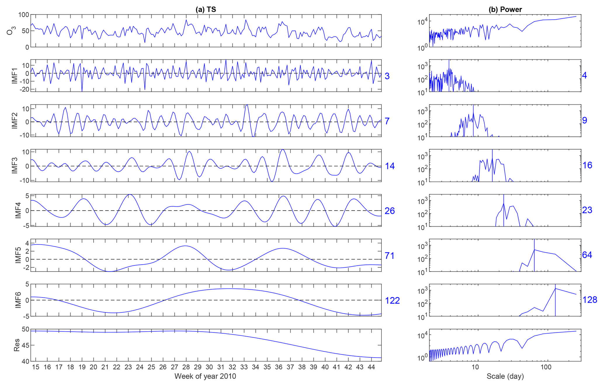
Figure 1Results of the application of the Improved CEEMDAN technique (a modified version of EMD), which is designed for analyzing non-stationary and non-linear time series (TS) data to the daily maximum 8 h ozone time series data at the Altoona, PA, site. The numbers on the right side represent the timescale (in days) associated with each IMF. Note that the power spectrum of raw ozone time series (upper right panel) shows that the energy in the 1–10 d (synoptic) timescale is an order of magnitude less than that in the longer (baseline) timescale.

Figure 2(a) Raw observed (OBS) DM8HR ozone time series (black) and the embedded baseline (BL; red for EMD and blue for KZ) at Altoona, PA, in 2010. (b) Time series of synoptic (SY) forcing (red for EMD and blue for KZ). Panels (c) and (d) show their corresponding power spectra. Panels (c) and (d) compare the power spectra of the baseline forcing (c) and the synoptic forcing (d) derived from KZ filtering and EMD (sum of IMF1 and IMF2). Notice that most of the energy in the baseline time series is in the longer timescale, while most of the energy of the short-term component is in the high-frequency range. The similarity of results from both scale separation techniques demonstrates that the two scales of interest (i.e., baseline and synoptic forcing) have been extracted reasonably well by these two methods.
3.1 Analysis of ambient ozone data
Using both Improved CEEMDAN and KZ filtering methods, we separated the synoptic forcing (timescale <24 d) and baseline (timescale >1 month) forcing embedded in the time series of observed and modeled daily maximum 8 h ozone concentrations. To illustrate, the results from the application of Improved CEEMDAN to the daily maximum 8 h ozone time series data measured at Altoona, PA, are presented in Fig. 1. The top left panel displays the raw ozone time series, while the top of the right panel shows its power spectrum. The seven intrinsic mode functions (IMFs) and the residual on the left side as well as their corresponding power spectra on the right reveal that most of the synoptic-scale features in ozone data are imbedded in IMFs 1 and 2. The baseline ozone is extracted by removing the first two IMFs from the raw ozone time series. To illustrate the concept of the ozone baseline, DM8HR time series measured in 2010 at Altoona, PA, are presented in Fig. 2a together with the embedded baseline concentration as extracted by the KZ5,5 and Improved CEEMDAN. It is evident that high ozone levels are always associated with the elevated baseline. The difference between the raw ozone time series and baseline, denoted as the short-term or synoptic forcing, is displayed in Fig. 2b. The power spectra, displayed in Fig. 2c and d, reveal both methods yielded good scale separation. Due to the good agreement between both scale separation techniques, only the results from the KZ filter are presented for the remainder of the paper.
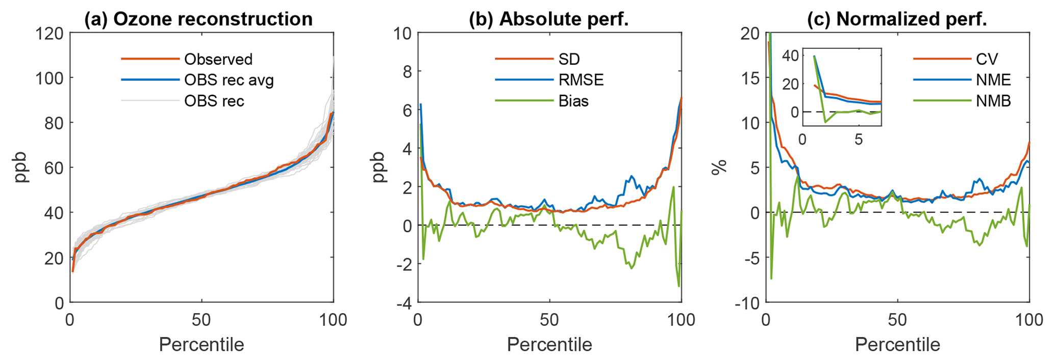
Figure 3(a) Comparison between the observed cumulative distribution function (CDF) for 2010 shown in red with 30+ pseudo-observation CDFs generated from historical DM8HR ozone time series shown in gray at a suburban site at Altoona, PA (AQS station identifier 420130801). The blue line represents the average of the 30+ gray lines. (b) Display of various statistical performance (perf.) metrics (standard deviation – std, root mean square error – RMSE, and bias) derived by comparing the actual observed and pseudo ozone values in panel (a). (c) Normalized statistical metrics of the normalized mean error (NME), normalized mean bias (NMB), and coefficient of variation (CV). Notice the large variability occurring at the lower and upper percentiles.
Once the scale separation is achieved with the KZ5,5, we superimposed the SY forcing imbedded in 30+ years of historical DM8HR ozone time series measured at a given location on the baseline component of the ozone time series at that location to generate 30+ reconstructed or pseudo ozone distributions. Illustrative results using Eq. (3) at a suburban location in Altoona, PA, are presented for the 2010 base year in Fig. 3a; it should be noted that the linear relationship between the strength of SY (defined as the standard deviation of the data in the synoptic component) and the magnitude of the BL (defined as the mean of the data in the baseline component) has been taken into account in generating 30+ years of adjusted SY forcing as illustrated in Luo et al. (2019). As expected, there is excellent agreement between the average of 30+ values (solid blue line) and observed ozone in 2010 at each percentile of the concentration distribution function (red line). Also, the original cumulative distribution function (CDF) in 2010 (red line) is constrained within the 30+ CDFs of pseudo distributions (Fig. 3a); note that it is equally likely for any of these 30+ CDFs to occur because of the stochastic nature of the atmosphere even though the individual event in 2010 yielded the CDF shown in red. As mentioned before, an ozone mixing ratio at any given probability point on the red line in Fig. 3a reflects an individual event, while ozone values at the same probability in different CDFs (gray lines) reflect the population stemming from the stochastic nature of the atmosphere. In other words, there are 30+ dynamically consistent ozone time series attributable to the 2010 baseline (given 2010 emissions) for examining the inherent variability due to atmospheric stochasticity. It is evident in Fig. 3a that there is larger variability at the lower and upper percentiles than that in interquartile range, revealing that the tails of the concentration distribution function are subject to large inherent uncertainty. Using these 30+ pseudo-observation ozone mixing ratios and the actual observed ozone values at each percentile, statistical metrics such as bias, the RMSE, the coefficient of variation (), the normalized mean error (NME), and the normalized mean bias (NMB) are presented in Fig. 3b and c (see Emery et al., 2016, for the description of the statistical metrics considered here). As expected, the lower and upper tails of the distribution are prone to large errors. These results demonstrate the presence of substantial natural variability at the upper 95th percentile, which is of primary interest in regulatory analyses. The extreme values are better described in statistical terms rather than in deterministic sense (Rao and Visalli, 1981; Hogrefe and Rao, 2001; Luo et al., 2019).

Figure 4Box plots of statistical metrics based on the results from the analysis of DM8HR data at 185 monitoring sites: (a) standard deviation, (b) root mean square error, (c) mean bias, (d) coefficient of variation, (e) normalized mean error, and (f) normalized mean bias. The lower and upper edges of the boxes represent the 25th and 75th percentile values, while the whiskers represent the 5th and 95th percentiles. See data analysis procedures using the ozone baseline observed in the year 2010 as the target baseline in Eqs. (7) and (8) of Luo et al. (2019).
Ozone time series at 185 monitoring stations covering CONUS, having at least 80 % data completeness, are analyzed in the above manner, and the results are displayed as box plots in Fig. 4. Note the presence of large variability in the CV, NME, NMB, and bias at the lower and upper percentiles (Fig. 4). The RMSE expected for the ozone mixing ratios in the interquartile range is ∼1.5 ppb, but it is >5 ppb for the upper 95th percentile (Fig. 4b). The spatial distribution of the RMSE at the 50th and 95th percentiles is displayed in Fig. 5a and b, respectively. The RMSE at the upper 95th percentile is very high at some monitoring sites in California and Michigan (Fig. 5b). Monitoring stations situated in the urban areas, near large bodies of water, and in regions of complex terrain influenced predominantly by local conditions tend to exhibit higher RMSE values. The elevation of the monitoring sites is displayed in Fig. 5c.
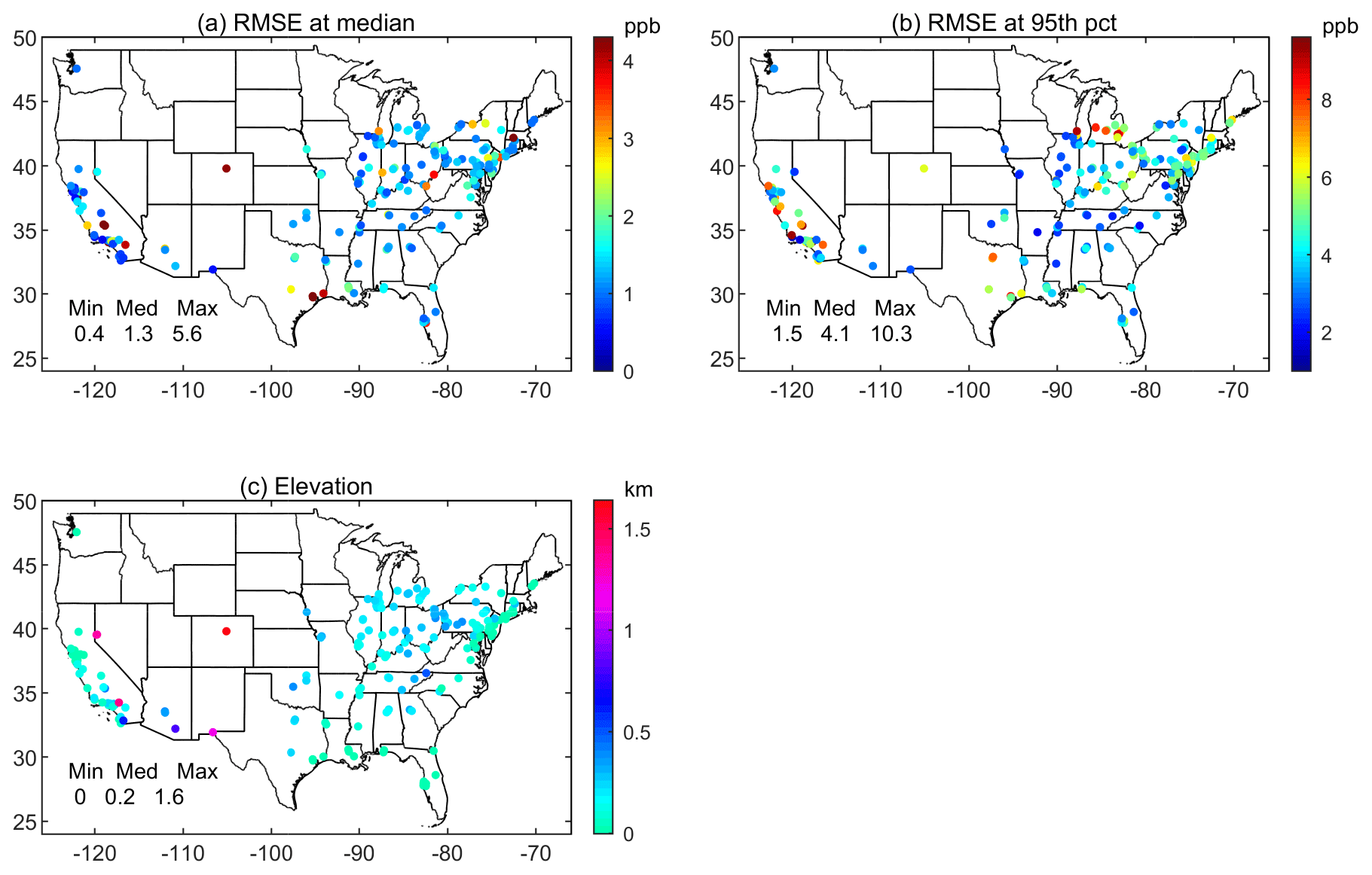
Figure 5Spatial distribution of the lower bound for the RMSE or expected RMSE at each monitoring site over CONUS (a) at the median and (b) at the 95th percentile. (c) Elevation (km) above the mean sea level of each monitoring site.
3.2 Analysis of modeled ozone concentrations
The analysis in the previous section quantified the inherent stochastic variability that is present in the SY component using long-term records of ozone observations. In this section, we analyze long-term records of model simulations in an attempt to quantify the error associated with the modeled SY component that results both from not explicitly representing stochastic variations in atmospheric dynamics in the current generation regional air quality models and from other reducible sources of model error. The model simulations were performed with the fully coupled WRF-CMAQ system with a 36 km horizontal grid cell size and covered the 21-year period from 1990 to 2010 (Gan et al., 2015). In this section, we examine the impact of superimposing different SY forcings embedded in ozone observations vs. those in the WRF-CMAQ model on the observed baseline concentration. To provide an illustration of the differences between observed and modeled time series over this period, Fig. 6a displays a scatter plot of the strength of the SY component (standard deviation of data in the SY component) vs. the mean of the baseline component for both observations and model simulations at the Altoona, PA, site. While both observations and WRF-CMAQ simulations show a strong correlation between these two variables, it is evident that at this monitoring location the standard deviation (i.e., strength) of the SY component is substantially lower for the WRF-CMAQ simulations for a given mean of the BL component (i.e., for any given year). The year-to-year variation in the observed and modeled mean of the BL and strength of SY forcing, displayed in Fig. 6b, reveals that the model overestimated the BL and underestimated the strength of SY forcing. The 36 km grid may be better for representing the large-scale synoptic forcing associated with the translation of weather systems than the meso-scale weather and urban influences (both dynamics and chemistry) that are embedded in the observed SY component. Meteorological modeling with higher horizontal grid resolution might be able to capture the land–sea breeze, lake–sea breeze, and terrain influences that observations are seeing at certain monitoring locations.
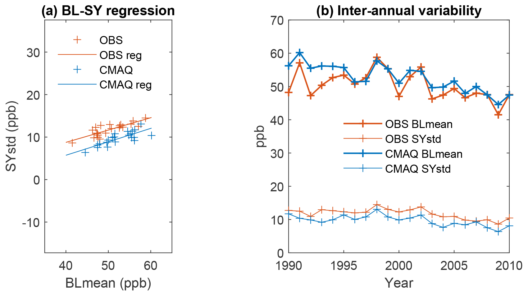
Figure 6(a) Scatter plot of the standard deviation (i.e., strength) of the synoptic (SY) component vs. the mean of the baseline (BL) component for each of the 21 years from 1990 to 2010 at the Altoona, PA, monitoring site. Observations are shown in red, while WRF-CMAQ results are shown in blue. (b) Inter-annual variability in the mean of the baseline component and standard deviation of the synoptic component in the WRF-CMAQ model and observations at the Altoona, PA, site. Although year-to-year variation is captured, the model has overestimated the baseline forcing and underestimated the synoptic forcing.
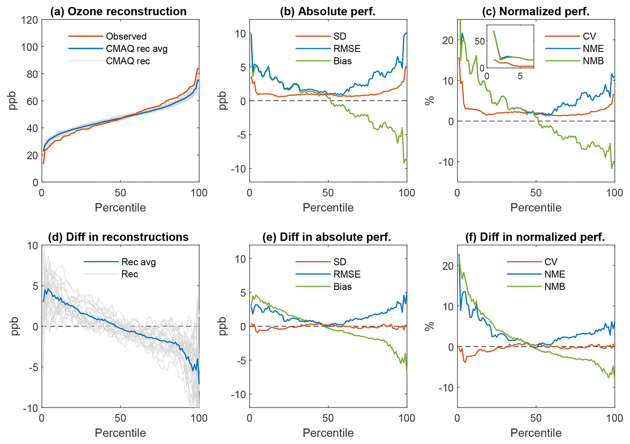
Figure 7(a) Comparison between the observed CDF overlaid on 21 “pseudo-simulated” or reconstructed ozone CDFs with SY generated from modeled DM8HR ozone time series at a suburban site at Altoona, PA (AQS station identifier 420130801). (b) Display of various statistical performance (perf.) metrics derived by comparing the actual observed and pseudo-simulated ozone values in panel (a). (c) Normalized statistical metrics. (d) Difference between the pseudo-simulated CDFs shown in panel (a) and the pseudo-observed CDFs as shown in panel (a) but calculated from 21 years (1990–2010) of observations only. The gray lines represent the differences for a specific SY year, while the blue line represents the differences between the means of the 21 reconstructions. (e) Difference between the absolute performance metrics for pseudo-simulations shown in panel (b) and those calculated for pseudo-observations as shown in panel (b) but calculated for 21 years (1990–2010) only. (f) As in panel (e) but for normalized performance metrics.
To isolate the impact of model imperfections on only the SY timescale on errors across the ozone distribution, we assume that the model perfectly reproduces the “true” BL depicted by the observed 2010 BL. We then use this perfect modeled BL and reconstruct “pseudo-simulated” ozone time series, like what was done in Fig. 3, except for using the SY component embedded in the 21 years of coupled WRF-CMAQ simulations. The rationale for this analysis is to quantify the amount of model error present in the current simulations that could conceivably be reduced through improving the representation of synoptic and mesoscale processes and/or increased horizontal resolution with appropriate data assimilation techniques. Figure 7a displays the CDF of actual observed ozone (red line) overlaid on 21 pseudo-simulated ozone CDFs (gray lines, with averages of all 21 pseudo-simulated ozone percentiles shown in blue) at the Altoona, PA, site, while Fig. 7b and c display absolute and normalized performance metrics. Figure 7a confirms that the coupled WRF-CMAQ SY components have less intra-annual variability than observed SY components, causing overestimation at the low end and underestimation at the high end of the observed CDF for all 21 years of reconstruction; these results imply that the model's results at the upper and lower percentiles will always tend to be unreliable or prone to large errors even when the baseline concentration is predicted perfectly. The U shape of the absolute and relative error curves in Fig. 7b and c is similar to the corresponding curves in Fig. 3, but the larger magnitude at the high and low end of the distribution indicates that the effects of the underestimated intra-annual SY variability (note that the distribution of modeled values in Fig. 7a is much flatter, i.e., with a higher kurtosis, than that of the observations) outweigh those errors attributable to the stochastic variability presented in Fig. 3. The shape of the absolute and normalized bias curves deviates from those shown for the pseudo-observations in Fig. 3b–c and, thus, this also reveals the effect of the underestimation of the intra-annual SY variability. Figure 7d–f present differences between the curves shown in Fig. 7a–c and a version of Fig. 3a–c computed from the 1990–2010 data instead of 30+ years of historical ozone observations. Panels (e) and (f) show that at the 50th percentile, the differences in the error curves are close to zero, since both the pseudo-simulations and pseudo-observations used the same observed BL component. At the upper percentiles, the differences reach 3–5 ppb, providing an estimate of the reducible error in simulating the extreme values at this location because of the differences in the observed SY and WRF-CMAQ SY components at this location; high-resolution meteorological modeling may help address these reducible errors.
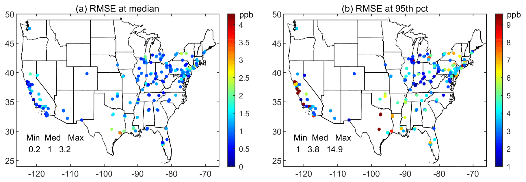
Figure 8Errors in the 21 “pseudo-simulated” or reconstructed ozone time series with SY generated from modeled DM8HR ozone time series using BL obtained from observations at (a) the median and (b) 95th percentile.
Figure 8a and b display the RMSE at the median and 95th percentile for the pseudo-simulated ozone values at each monitoring site. For the 50th percentile, the RMSE values range from 0.2 to 3.2 ppb over CONUS with a median value of 1 ppb, while at the 95th percentile, the RMSE values range from 1 to 15 ppb with a median value of 4 ppb across all sites over CONUS. The values are highest along the California coast and near Great Lakes, possibly due to inadequacies in simulating the land–sea breeze and land–lake breeze regimes, respectively, with modeling at 36 km grid cells. Air quality modeling uncertainty even for the retrospective modeling cases, outside of the chemistry formulation and boundary conditions, is attributed primarily to meteorology and emissions inputs. Vautard et al. (2012) and McNider and Pour-Biazar (2020) concluded that major challenges remain in the simulation of prevailing meteorology (e.g., errors in wind speed, PBL, night-time meteorology, nocturnal transport aloft, and clouds) in retrospective air quality modeling. Based on the retrospective ozone episodic modeling with the WRF-CMAQ model using various sets of equally likely initial conditions for meteorology along with FDDA, Gilliam et al. (2015) confirmed the presence of sizable spread in WRF solutions, including common weather variables of temperature, wind, boundary layer depth, clouds, and radiation, thereby causing a relatively large range of ozone concentrations. Also, pollutant transport is altered by hundreds of kilometers over several days. Ozone concentrations of the ensemble varied by as much as 10–20 ppb (or 20 %–30 %) in areas that typically have higher pollution levels. As model improvements are made, one can quantitatively assess how close the predictions of the improved model are for each percentile for the given base year simulation to the expected errors from a perfect model with perfect input, i.e., the target RMSE shown in Fig. 5a and b. Perhaps, the next generation of regional-scale meteorological and air quality models might be capable of explicitly simultaneously treating the mean and fluctuation components for all variables within the deterministic–stochastic modeling framework to properly account for the stochastic nature of the atmosphere.
Regardless of how accurate the regional air quality model is, the stochastic variations in the atmosphere cannot be consistently reproduced by the deterministic numerical models. In this study, we demonstrate how to quantify this irreproducible stochastic component by isolating the synoptic forcing imbedded in 30+ years of historical observations and assess the performance of the 36 km fully coupled WRF-CMAQ model in simulating 21 years of ozone concentrations over the contiguous US. Observation-based analysis reveals that on average, the irreducible error attributable to the stochastic nature of the atmosphere ranges from ∼2 ppb at the 50th percentile to ∼5 ppb at the 95th percentile. To improve regional-scale ozone air quality models, attention should be paid to accurately simulate the baseline concentration by focusing on the quality of the emission inventory and the model's treatment for the boundary conditions and slow-changing (operating on sub-seasonal, seasonal, and longer-term timescales) atmospheric processes. Also, errors in reproducing the synoptic forcing can possibly be reduced with high-resolution meteorological modeling using appropriate data assimilation techniques. Nonetheless, these results demonstrate the presence of large variability in the upper tail of the DM8HR O3 concentration cumulative distribution even with perfect models using perfect input data. Having this quantitative estimation of practical limits for a model's accuracy helps in objectively assessing the current state of regional-scale air quality models, measuring progress in their evolution, and providing meaningful and firm targets for improvements in their accuracy relative to measurements from routine networks.
Source code for version 5.0.2 of the Community Multiscale Air Quality (CMAQ) modeling system can be downloaded from https://github.com/USEPA/CMAQ/tree/5.0.2 (last access: 3 February 2020) (US EPA Office of Research and Development, 2014, https://doi.org/10.5281/zenodo.1079898). For further information, please visit the U.S. Environmental Protection Agency website for the CMAQ system at https://www.epa.gov/cmaq (last access: 3 February 2020).
All ozone observations used in this article are available from https://aqs.epa.gov/aqsweb/airdata/download_files.html (AQS) (last access: 3 February 2020). Paired ozone observation and CMAQ model data used in the analysis will be made available at https://edg.epa.gov/metadata/catalog/main/home.page (last access: 3 February 2020). Raw CMAQ model outputs are available on request from the EPA authors.
STR conceptualized the idea. STR, CH, VG, and RM designed the analysis approach. CH and RM post-processed previously conducted model simulations. HL performed data analyses and prepared the illustrations. STR prepared the paper with contributions from all co-authors.
The authors declare that they have no conflict of interest.
The views expressed in this paper are those of the authors and do not necessarily represent the view or policies of the U.S. Environmental Protection Agency.
The authors thank the reviewers for their constructive comments that have helped improve the paper.
This paper was edited by Leiming Zhang and reviewed by two anonymous referees.
Appel, K. W., Chemel, C., Roselle, S. J., Francis, X. V., Hu, R.-M., Sokhi, R. S., Rao, S. T., and Galmarini, S.: Examination of the Community Multiscale Air Quality (CMAQ) model performance over the North American and European domains. Atmospheric Environment, AQMEII: An International Initiative for the Evaluation of Regional-Scale Air Quality Models – Phase 1, 53, 142–155, https://doi.org/10.1016/j.atmosenv.2011.11.016, 2012.
Astitha, M., Luo, H., Rao, S. T., Hogrefe, C., Mathur, R., and Kumar, N.: Dynamic evaluation of two decades of WRF-CMAQ ozone simulations over the contiguous United States, Atmos. Environ., 164, 102–116, https://doi.org/10.1016/j.atmosenv.2017.05.020, 2017.
Baklanov, A., Schlünzen, K., Suppan, P., Baldasano, J., Brunner, D., Aksoyoglu, S., Carmichael, G., Douros, J., Flemming, J., Forkel, R., Galmarini, S., Gauss, M., Grell, G., Hirtl, M., Joffre, S., Jorba, O., Kaas, E., Kaasik, M., Kallos, G., Kong, X., Korsholm, U., Kurganskiy, A., Kushta, J., Lohmann, U., Mahura, A., Manders-Groot, A., Maurizi, A., Moussiopoulos, N., Rao, S. T., Savage, N., Seigneur, C., Sokhi, R. S., Solazzo, E., Solomos, S., Sørensen, B., Tsegas, G., Vignati, E., Vogel, B., and Zhang, Y.: Online coupled regional meteorology chemistry models in Europe: current status and prospects, Atmos. Chem. Phys., 14, 317–398, https://doi.org/10.5194/acp-14-317-2014, 2014.
Biswas, J. and Rao, S. T.: Uncertainties in episodic ozone modeling stemming from uncertainties in the meteorological fields, J. Appl. Meteor., 40, 117–136, 2001.
Bocquet, M., Elbern, H., Eskes, H., Hirtl, M., Žabkar, R., Carmichael, G. R., Flemming, J., Inness, A., Pagowski, M., Pérez Camaño, J. L., Saide, P. E., San Jose, R., Sofiev, M., Vira, J., Baklanov, A., Carnevale, C., Grell, G., and Seigneur, C.: Data assimilation in atmospheric chemistry models: current status and future prospects for coupled chemistry meteorology models, Atmos. Chem. Phys., 15, 5325–5358, https://doi.org/10.5194/acp-15-5325-2015, 2015.
Carmichael, G. R., Sakurai, T., Streets, D., Hozumi, Y., Ueda, H., Park, S. U., Fung, C., Han, Z., Kajino, M., Engardt, M., Bennet, C., Hayami, H., Sartelet, K., Holloway, T., Wang, Z., Kannari, A., Fu, J., Matsuda, K., Thongboonchoo, N., and Amann, M.: MICS-Asia II: The model intercomparison study for Asia Phase II methodology and overview of findings, Atmos. Environ., 42, 3468–3490, https://doi.org/10.1016/j.atmosenv.2007.04.007, 2008.
Colominas, M. A., Schlotthauer, G., and Torres, M. E.: Improved complete ensemble EMD: A suitable tool for biomedical signal processing, Biomed. Signal Proces., 14, 19–29, 2014.
Demerjian, K. L.: Quantifying Uncertainty in Long-Range-Transport Models: A Summary of the AMS Workshop on Sources and Evaluation of Uncertainty in Long-Range-Transport Models, B. Am. Meteorol. Soc., 66, 1533–1540, 1985.
Dennis, R., Fox, T., Fuentes, M., Gilliland, A., Hanna, S., Hogrefe, C., Irwin, J., Rao, S. T., Scheffe, R., Schere, K., Steyn, D., and Venkatram, A.: A framework for evaluating regional-scale numerical photochemical modeling systems, Environ. Fluid Mech., 10, 471–489, https://doi.org/10.1007/s10652-009-9163-2, 2010.
Emery, C., Liu, Z., Russell, A. G., Talat Odman, M., Yarwood, G., and Kumar, N.: Recommendations on statistics and benchmarks to assess photochemical model performance, J. Air Waste Manage. Assoc., 67, 582–598, https://doi.org/10.1080/10962247.2016.1265027, 2016.
Foley, K. M., Napelenok, S. L., Jang, C., Phillips, S., Hubbell, B. J., and Fulcher, C. M.: Two reduced form air quality modeling techniques for rapidly calculating pollutant mitigation potential across many sources, locations and precursor emission types, Atmos. Environ., 98, 283–289, https://doi.org/10.1016/j.atmosenv.2014.08.046, 2014.
Fox, D. G.: Judging Air Quality Model Performance: A Summary of the AMS Workshop on Dispersion Model Performance, Douglas O. box Woods Hole, Mass., 8–11 September 1980, B. Am. Meteorol. Soc., 62, 599–609, 1981.
Fox, D. G.: Uncertainty in Air Quality Modeling A Summary of the AMS Workshop on Quantifying and Communicating Model Uncertainty, Woods Hole, Mass., September 1982, 65, 27–36, 1984.
Gan, C.-M., Pleim, J., Mathur, R., Hogrefe, C., Long, C. N., Xing, J., Wong, D., Gilliam, R., and Wei, C.: Assessment of long-term WRF–CMAQ simulations for understanding direct aerosol effects on radiation “brightening” in the United States, Atmos. Chem. Phys., 15, 12193–12209, https://doi.org/10.5194/acp-15-12193-2015, 2015.
Gilliam, R. C., Hogrefe, C., and Rao, S. T.: New methods for evaluating meteorological models used in air quality applications, Atmos. Environ., 40, 5073–5086, 2006.
Gilliam, R. C., Godowitch, J., and Rao, S. T.: Diagnostic evaluation of ozone production and horizontal transport in a regional photochemical air quality modeling system, Atmos. Environ., 53, 3977–3987, https://doi.org/10.1016/j.atmosenv.2011.04.062, 2012.
Gilliam, R. C., Hogrefe, C., Godowitch, G., Napelenok, S., Mathur, R., and Rao, S. T.: Impact of inherent meteorology uncertainty on air quality model predictions, J. Geophys. Res.-Atmos., 120, 12259–12280, https://doi.org/10.1002/2015JD023674, 2015.
Grell, G. and Baklanov, A.: Integrated modeling for forecasting weather and air quality: A call for fully coupled approaches, Atmos. Environ., 45, 6845–6851, https://doi.org/10.1016/j.atmosenv.2011.01.017, 2011.
Herwehe, J. A., Otte, T. L., Mathur, R., and Rao, S. T.: Diagnostic analysis of ozone concentrations simulated by two regional-scale air quality models, Atmos. Environ., 45, 5957–5969, 2011.
Hogrefe, C. and Rao, S. T.: Demonstrating attainment of the air quality standards: Integration of observations and model predictions into the probabilistic framework, J. Air Waste Manage. Assoc., 51, 1060–1072, https://doi.org/10.1080/10473289.2001.10464332, 2001.
Hogrefe, C., Rao, S. T., Zurbenko, I. G., and Porter, P. S.: Interpreting the Information in Ozone Observations and Model Predictions Relevant to Regulatory Policies in the Eastern United States, B. Am. Meteorol. Soc., 81, 2083–2106, https://doi.org/10.1175/1520-0477(2000)081<2083:ITIIOO>2.3.CO;2, 2000.
Hogrefe, C., Rao, S. T., Kasibhatla, P., Hao, W., Sistla, G., Mathur, R., and McHenry, J.: Evaluating the performance of regional-scale photochemical modeling systems: Part II – ozone predictions, Atmos. Environ., 35, 4175–4188, https://doi.org/10.1016/S1352-2310(01)00183-2, 2001a.
Hogrefe, C., Rao, S. T., Kasibhatla, P., Kallos, G., Tremback, C. J., Hao, W., Olerud, D., Xiu, A., McHenry, J., and Alapaty, K.: Evaluating the performance of regional-scale photochemical modeling systems: Part I – meteorological predictions, Atmos. Environ., 35, 4159–4174, https://doi.org/10.1016/S1352-2310(01)00182-0, 2001b.
Hogrefe, C., Vempaty, S., Rao, S. T., and Porter, P. S.: A comparison of four techniques for separating different time scales in atmospheric variables, Atmos. Environ., 37, 313–325, https://doi.org/10.1016/S1352-2310(02)00897-X, 2003.
Hogrefe, C., Ku, J. Y., Sistla, G., Gilliland, A., Irwin, J. S., Porter, P. S., Gégo, E., and Rao, S. T.: How has model performance for regional scale ozone simulations changed over the past decade?, Air Pollution Modeling and its Application XIX, edited by: Borrego, C. and Miranda, A. I., Springer, Dordrecht, the Netherlands, pp. 394–403, 2008.
Hogrefe, C., Pouliot, G., Wong, D., Torian, A., Roselle, S., Pleim, J., and Mathur, R.: Annual application and evaluation of the online coupled WRF–CMAQ system over North America under AQMEII phase 2, Atmos. Environ., 115, 683–694, https://doi.org/10.1016/j.atmosenv.2014.12.034, 2015.
Huang, N. E., Shen, Z., Long, S. R., Wu, M. C., Shih, H. H., Zheng, Q., Yen, N. C., Tung, C. C., and Liu, H. H.: The empirical mode decomposition and the Hilbert spectrum for nonlinear and non-stationary time series analysis, P. Roy. Soc. Lond. A Mat., 454, 903–995, https://doi.org/10.1098/rspa.1998.0193, 1998.
Kang, D., Hogrefe, C., Foley, K., Napelenok, S., Mathur, R., and Rao, S. T.: Application of the Kolmogorov–Zurbenko filter and the decoupled direct 3D method for the dynamic evaluation of a regional air quality model, Atmos. Environ., 80, 58–69, https://doi.org/10.1016/j.atmosenv.2013.04.046, 2013.
Lamb, R. G.: Air pollution models as descriptors of cause-effect relationships, Atmos. Environ., 18, 591–606, 1984.
Lamb, R. G. and Hati, S. K.: The representation of atmospheric motions in models of regional-scale air pollution, J. Climatol. Appl. Meteor., 26, 837–846, 1987.
Lau, K.-M. and Weng, H.-Y.: Climate signal detection using wavelet transform: how to make a time series sing, B. Am. Meteorol. Soc., 76, 2391–2402, 1995.
Lee, A. M., Carver, G. D., Chipperfield, M. P., and Pyle, P. A.: Three-dimensional chemical forecasting: A methodology, J. Geophys. Res., 102, 3905–3919, 1997.
Lewellen, W. S. and Sykes, R. I.: Meteorological data needs for modeling air quality uncertainties, J. Atmos. Ocean. Tech., 6, 759–768, 1989.
Luo, H., Astitha, M., Hogrefe, C., Mathur, R., and Rao, S. T.: A new method for assessing the efficacy of emission control strategies, Atmos. Environ., 199, 233–243, https://doi.org/10.1016/j.atmosenv.2018.11.010, 2019.
Mathur, R., Xing, J., Gilliam, R., Sarwar, G., Hogrefe, C., Pleim, J., Pouliot, G., Roselle, S., Spero, T. L., Wong, D. C., and Young, J.: Extending the Community Multiscale Air Quality (CMAQ) modeling system to hemispheric scales: overview of process considerations and initial applications, Atmos. Chem. Phys., 17, 12449–12474, https://doi.org/10.5194/acp-17-12449-2017, 2017.
McNair, L. A., Harley, R. A., and Russell, A. G.: Spatial inhomogeneity in pollutant concentrations, and their implications for air quality model evaluation, Atmos. Environ., 30, 4291–4301, https://doi.org/10.1016/1352-2310(96)00098-2, 1996.
McNider, R. T. and Pour-Biazar, A.: Meteorological modeling relevant to mesoscale and regional air quality applications: A Review, J. Air Waste Manage. Assoc., 70, 2–43, https://doi.org/10.1080/10962247.2019.1694602, 2020.
Napelenok, S., Foley, K., Kang, D., Mathur, R., Pierce, T., and Rao, S. T.: Dynamic evaluation of regional air quality model's response to emission reductions in the presence of uncertain emission inventories, Atmos. Environ., 45, 4091–4098, https://doi.org/10.1016/j.atmosenv.2011.03.030, 2011.
Oreskes, N., Shrader-Frechette, K., and Belitz, K.: Verification, Validation, and Confirmation of Numerical Models in the Earth Sciences, Science, 263, 641–646, https://doi.org/10.1126/science.263.5147.641, 1994.
Pielke, R. A.: The need to assess uncertainty in air quality evaluations, Atmos. Environ., 32, 1467–1468, 1998.
Pierce, T., Hogrefe, C., Rao, S. T., Porter, P. S., and Ku, J.-Y.: Dynamic evaluation of a regional air quality model: Assessing the emissions-induced weekly ozone cycle, Atmos. Environ., 44, 3583–3596, 2010.
Pinder, R. W., Gilliam, R. C., Appel, K. W., Napelenok, S., Foley, K. M., and Gilliland, A. B.: Efficient Probabilistic Estimates of Surface Ozone Concentration Using an Ensemble of Model Configurations and Direct Sensitivity Calculations, Environ. Sci. Technol., 43, 2388–2393, 2008.
Porter, P. S., Rao, S. T., Hogrefe, C., Gego, E., and Mathur, R.: Methods for reducing biases and errors in regional photochemical model outputs for use in emission reduction and exposure assessments, Atmos. Environ., 112, 178–188, https://doi.org/10.1016/j.atmosenv.2015.04.039, 2015.
Poularika, A. D.: The Handbook of Formulas and Tables for Signal Processing, CRC Press, Boca Raton, FL, 1998.
Rao, S. T. and Visalli, J.: On the comparative assessment of the performance of air quality models, J. Air Poll. Contr. Assoc., 31, 851–860, https://doi.org/10.1080/00022470.1981.10465286, 1981.
Rao, S. T. and Zurbenko, I. G.: Detecting and Tracking Changes in Ozone Air Quality, Air Waste, 44, 1089–1092, https://doi.org/10.1080/10473289.1994.10467303, 1994.
Rao, S. T., Sistla, G., Pagnotti, V., Petersen, W. B., Irwin, J. S., and Turner, D. B.: Resampling and Extreme Value Statistics in Air Quality Model Performance Evaluation, Atmos. Environ., 19, 1503–1518, 1985.
Rao, S. T., Zurbenko, I. G., Porter, P. S., Ku, J.-Y., and Henry, R. F.: Dealing with the ozone non-attainment problem in the Eastern United States, Environ. Manage., 1996, 17–31, 1996.
Rao, S. T., Zurbenko, I. G., Neagu, R., Porter, P. S., Ku, J. Y., and Henry, R. F.: Space and Time Scales in Ambient Ozone Data, B. Am. Meteorol. Soc., 78, 2153–2166. https://doi.org/10.1175/1520-0477(1997)078<2153:SATSIA>2.0.CO;2, 1997.
Rao, S. T., Galmarini, S., and Pucket, K.: Air Quality Model Evaluation International Initiative (AQMEII)-Advancing the State of the Science in Regional Photochemical Modeling and Its Applications, B. Am. Meteorol. Soc., 2011, 23–30, https://doi.org/10.1175/2010BAMS3069.1, 2011a.
Rao, S. T., Porter, P. S., Mobley, J. D., and Hurley, F.: Understanding the spatio-temporal variability in air pollution concentrations, Environ. Manage., 70, 42–48, 2011b.
Ryan, W. F.: The air quality forecast rote: Recent changes and future challenges, J. Air Waste Manage. Assoc., 66, 576–596, https://doi.org/10.1080/10962247.2016.1151469, 2016.
Sarwar, G., Godowitch, J., Henderson, B. H., Fahey, K., Pouliot, G., Hutzell, W. T., Mathur, R., Kang, D., Goliff, W. S., and Stockwell, W. R.: A comparison of atmospheric composition using the Carbon Bond and Regional Atmospheric Chemistry Mechanisms, Atmos. Chem. Phys., 13, 9695–9712, https://doi.org/10.5194/acp-13-9695-2013, 2013.
Simon, H., Baker, K. R., and Phillips, S.: Compilation and interpretation of photochemical model performance statistics published between 2006 and 2012, Atmos. Environ., 61, 124–139, 2012.
Solazzo, E. and Galmarini, S.: Comparing apples with apples: Using spatially distributed time series of monitoring data for model evaluation, Atmos. Environ., 112, 234–245, https://doi.org/10.1016/j.atmosenv.2015.04.037, 2015a.
Solazzo, E. and Galmarini, S.: A science-based use of ensembles of opportunities for assessment and scenario studies, Atmos. Chem. Phys., 15, 2535–2544, https://doi.org/10.5194/acp-15-2535-2015, 2015b.
Solazzo, E., Bianconi, R., Matthias, V., Vautard, R., Moran, M. D., Appell, K. A., Bessagnet, B., Brandt, S. J., Chemel, C., Coll, I., Ferrera, J., Forkel, R., Francis, X., Grell, G., Grossi, G., Hansen, A., Galmarini, S., Prank, M., Sartelet, K., Schaap, M., Silver, J., Sokhi, R., Vira, J., Werhahn, J., Wolke, R., Yarwood, G., Zhange, J., Rao, S. T., and Galmarini, S.: Operational model evaluation for particulate matter in Europe and North America in the context of AQMEII, Atmos. Environ., 53, 75–92, 2012.
Stockwell, W. R., Saunders, E., Goliff, W. S., and Fitzgerald, R. M.: A perspective on the development of gas-phase chemical mechanisms for Eulerian air quality models, J. Air Waste Manage. Assoc., 70, 44–70, https://doi.org/10.1080/10962247.2019.1694605, 2020.
Swall, J. L. and Foley, K. M.: The impact of spatial correlation and incommensurability on model evaluation, Atmos. Environ., 43, 1204–1217, https://doi.org/10.1016/j.atmosenv.2008.10.057, 2009.
Thomas, A., Huff, A. K., Hu, X.-M., and Zhang, F.: Quantifying uncertainties of ground-level ozone within WRF-Chem simulations in the mid-Atlantic region of the United States as a response to variability, J. Adv. Model. Earth Syst., 11, 1100–1116, https://doi.org/10.1029/2018MS001457, 2019.
U.S. Environmental Protection Agency: Modeling Guidance for Demonstrating Air Quality Goals for Ozone, PM2.5, and Regional Haze, EPA 454/R-18-009, 203 pp., available at: https://www3.epa.gov/ttn/scram/guidance/guide/O3-PM-RH-Modeling_Guidance-2018.pdf (last access: 3 February 2020), 2018.
US EPA Office of Research and Development: CMAQv5.0.2 (Version 5.0.2), Zenodo, https://doi.org/10.5281/zenodo.1079898, 2014.
Vautard, R., Moran, M. D., Solazzo, E., Gilliam, R., Mathias, V., Bianconi, R., Chemel, C., Ferreira, J., Geyer, B., Hansen, A. B., Jericevic, A., Prank, M., Segers, A., Silver, J. D., Werhahn, J., Wolke, Rao, S. T., and Galmarini, S.: Evaluation of the meteorological forcing used for the Air Quality Model Evaluation International Initiative (AQMEII) air quality simulations, Atmos. Environ., 53, 15–37, https://doi.org/10.1016/j.atmosenv.2011.10.065, 2012.
Vukovich, F. M.: Time Scales of Surface Ozone Variations in the Regional, Non-URBAN Environment, Atmos. Environ., 31, 1513–1530, 1997.
Wilmott, C. J.: On the Validation of Models, Phys. Geogr., 2, 184–194, https://doi.org/10.1080/02723646.1981.10642213, 1981.
Wilmott, C., Ackleson, S., Davis, R., Feddema, J., Klink, K., Legates, R., O'Donnell, R., and Rowe, C.: Statistics for the Evaluation and Comparison of Models, J. Geophys. Res., 90, 8995–9005, 1985.
Xing, J., Mathur, R., Pleim, J., Hogrefe, C., Gan, C.-M., Wong, D. C., Wei, C., Gilliam, R., and Pouliot, G.: Observations and modeling of air quality trends over 1990–2010 across the Northern Hemisphere: China, the United States and Europe, Atmos. Chem. Phys., 15, 2723–2747, https://doi.org/10.5194/acp-15-2723-2015, 2015.
Xing, J., Mathur, R., Pleim, J., Hogrefe, C., Wang, J., Gan, C.-M., Sarwar, G., Wong, D. C., and McKeen, S.: Representing the effects of stratosphere–troposphere exchange on 3-D O3 distributions in chemistry transport models using a potential vorticity-based parameterization, Atmos. Chem. Phys., 16, 10865–10877, https://doi.org/10.5194/acp-16-10865-2016, 2016.
Ying, Y. and Zhang, F.: Potentials in improving predictability of multiscale tropical weather systems evaluated through ensemble assimilation of simulated satellite-based observations, J. Atmos. Sci., 75, 1675–1697, https://doi.org/10.1175/JAS-D-17-0245.1, 2018.
Zhang, Y., Hong, C. P., Yahya, K., Li, Q., Zhang, Q., and He, K.-B.: Comprehensive evaluation of multi-year real-time air quality forecasting using an online-coupled meteorology-chemistry model over southeastern United States, Atmos. Environ., 138, 162–182, https://doi.org/10.1016/j.atmosenv.2016.05.006, 2016.
Zurbenko, I. G., Porter, P. S., Gui, R., Rao, S. T., Ku, J. Y., and Eskridge, R. E.: Detecting discontinuities in time series of upper-air data: Development and demonstration of an adaptive filter technique, J. Climate, 9, 3548–3560, https://doi.org/10.1175/1520-0442(1996)009<3548:DDITSO>2.0.CO;2, 1996.