Spatial and temporal representativeness of point measurements for nitrogen dioxide pollution levels in cities

In many cities around the world the overall air quality is improving, but at the same time nitrogen dioxide (NO₂) trends show stagnating values and in many cases could not be reduced below air quality standards recommended by the World Health Organization (WHO). Many large cities have built monitoring stations to continuously measure different air pollutants. While most stations follow defined rules in terms of measurement height and distance to traffic emissions, the question remains of how representative are those point measurements for the city-wide air quality. The question of the spatial coverage of a point measurement is important because it defines the area of influence and coverage of monitoring networks, determines how to assimilate monitoring data into model simulations or compare to satellite data with a coarser resolution, and is essential to assess the impact of the acquired data on public health.

In order to answer this question, we combined different measurement data sets consisting of path-averaging remote sensing data and in situ point measurements in stationary and mobile setups from a measurement campaign that took place in Munich, Germany, in June and July 2016. We developed an algorithm to strip temporal from spatial patterns in order to construct a consistent NO₂ pollution map for Munich. Continuous long-path differential optical absorption spectroscopy (LP DOAS) measurements were complemented with mobile cavity-enhanced (CE) DOAS, chemiluminescence (CL) and cavity attenuated phase shift (CAPS) instruments and were compared to monitoring stations and satellite data. In order to generate a consistent composite map, the LP DOAS diurnal cycle has been used to normalize for the time of the day dependency of the source patterns, so that spatial and temporal patterns can be analyzed separately. The resulting concentration map visualizes pollution hot spots at traffic junctions and tunnel exits in Munich, providing insights into the strong spatial variations. On the other hand, this database is beneficial to the urban planning and the design of control measures of environment pollution. Directly comparing on-street mobile measurements in the vicinity of monitoring stations resulted in a difference of 48 %. For the extrapolation of the monitoring station data to street level, we determined the influence of the measuring height and distance to the street. We found that a measuring height of 4 m, at which the Munich monitoring stations measure, results in 16 % lower average concentrations than a measuring height of 1.5 m, which is the height of the inlet of our mobile measurements and a typical pedestrian breathing height. The horizontal distance of most stations to the center of the street of about 6 m also results in an average reduction of 13 % compared to street level concentration. A difference of 21 % in the NO₂ concentrations remained, which could be an indication that city-wide measurements are needed for capturing the full range and variability of concentrations for assessing pollutant exposure and air quality in cities.

1 Introduction

Many former studies (Huang et al., 2014; Dunlea et al., 2007; Jang and Kamens, 2001) have been pointed out that NO₂ is an important composition in the process of both tropospheric and stratospheric chemistry. It is one of the major pollution products from combustion processes. Catalytic formation of tropospheric ozone (O₃) and the formation of secondary aerosols that cause acid rain, all of which involve its participation. Elevated concentration of atmospheric NO₂ is acknowledged to be noxious to human beings' health. In urban environments, exhaust emissions are one of the primary sources of air pollution, particularly NO_x (= NO+NO₂). Nitrogen monoxide (NO) accounts for the majority of direct traffic emissions, which is subsequently oxidized to form NO₂ although some NO₂ is emitted directly (Ban-Weiss et al., 2008; Henderson et al., 2007; Kirchstetter et al., 1999). NO₂ levels are often strongly correlated with many other toxic air pollutants (Massman, 1998; Yoo et al., 2014; Xie et al., 2015). Its concentration can be easily and precisely measured, which is helpful in assessing general air quality. Since it is a short-lived compound gas from numerous different sources, its concentrations can vary strongly, both in space and time.

According to the 2017 European Environment Agency report (EEA, 2017), some NO₂ concentrations measured at air quality monitoring stations are above the World Health Organization (WHO) Air Quality Guideline (AQG) values of 200 µg m⁻³ (hourly) and 40 µg m⁻³ (annually). A total of 10.5 % of the stations across European cities exceeded the annual limits, including several German cities. None of the exceedances were observed at rural background stations but instead in urban or suburban stations. More specifically, 89 % of the exceeded values were observed at traffic stations. The 2016 air quality report by the German Environment Agency (Umweltbundesamt) (UBA, 2017) also pointed out that the air pollution in urban conurbations was primarily affected by traffic. In the 2015 technical report by the Bavarian environment agency (Landesamt für Umwelt, LfU) (LfU, 2015), the on-road NO₂ concentration limits were exceeded in most Bavarian cities from 2000 to 2014. In particular, the annual NO₂ level in Munich measured at Landshuter Allee station was more than twice the annual NO₂ limit value of the WHO AQG of 40 µg m⁻³.

With a growing focus on air pollution in the public attention, stationary monitoring networks have been established all over the world. Related regulations also have been certified. For example, in Europe, the European directive 2008/50/EC lists a number of criteria for microscale positioning of air quality measurements (Annex III section C). Monitoring stations in the EU continuously measure different pollutants, and while most stations follow the defined rules in terms of measurement height and distance to traffic emissions, the question remains of how representative are those point measurements for the city-wide air quality. According to a study of the spatial distribution of NO₂ in Hong Kong (Zhu et al., 2018), large differences between mobile measurements around the city and seven local monitoring stations were observed. In order to determine the representativeness of air quality monitoring stations, different measurement methods have to be combined. Most monitoring stations utilize the chemiluminescence (CL) technique for NO_x measurements. Thereby the NO₂ concentration is determined indirectly by calculating the difference between NO_x and NO concentrations. The concentration of oxidized odd-Nitrogen species (NO_y) is inevitably included as a small measurement error. Nevertheless, the CL technique has a good detection sensitivity that is given by its low background signal. This is because for initiating the fluorescence no light source is required (Dunlea et al., 2007). In this study, we compared our CL and cavity-enhanced DOAS (CE DOAS) data to the local air quality stations and studied the diffusion rate of NO₂ in both vertical and horizontal directions from one of the stations.

For our study we utilized a combination of a long-path DOAS (LP DOAS) instrument and a CE DOAS, as well as a cavity attenuated phase shift spectroscopy (CAPS) instrument to determine the spatiotemporal variability of NO₂ concentrations in the central area of Munich. CE DOAS is a spectroscopic measurement technique that uses an optical resonator to fold the absorption path into a resonator (Zhu et al., 2018; Min et al., 2016; Thalman and Volkamer, 2010; Platt et al., 2009; Washenfelder et al., 2008; Venables et al., 2006; Langridge et al., 2006). CAPS (Herbelin et al., 1980) is a spectroscopic detection technology, generally referred to as cavity-enhanced optical absorption, which has also been applied for the detection of atmospheric pollutants in many studies (Xie et al., 2019; Kundu et al., 2019; Ge et al., 2013; Kebabian et al., 2005a, 2008). The advantage of CE DOAS and CAPS is the fact that they are not sensitive to other reactive nitrogen oxides in the atmosphere like some other in situ NO₂ monitoring techniques. They are both characterized by a compact setup and have no sensitivity loss during the operation. For mobile measurements a fast sampling rate is necessary, and the high accuracy of the instruments allowed a sampling rate of 2 s. Similar instrument setups have been used in many on-road studies of vehicles emissions (Zhu et al., 2018; Chan et al., 2017; Rakowska et al., 2014; Ning et al., 2012; Uhrner et al., 2007; Vogt et al., 2003).

For our study we conducted on-road measurements of NO₂ concentrations in June and July 2016 in order to investigate street level air quality and locate emission hot spot areas. Additionally, LP DOAS measurements were conducted to observe the temporal variability of ambient NO₂ in Munich. A measurement system consisting of several DOAS instruments was continuously operational for over 2 years (see Sect. 2). The algorithm that combines the mobile and stationary measurement data is described in Sect. 3.1.1. The resulting on-road NO₂ spatial patterns are presented in Sect. 3.1.2. The CE DOAS and CL were set up next to the Bavarian LfU local air quality station to measure the horizontal and vertical NO₂ distributions, and the results are shown in Sect. 3.2. NO₂ data from the Ozone Monitoring Instrument (OMI) on board the NASA Aura satellite were used to verify how the LP DOAS measurements compare to the much larger OMI ground pixels covering a larger fraction of the city in order to find out whether the LP DOAS measurements are representative for the whole city. Detailed analysis is provided in the Supplement.

2 Methodology

This study combines different measurement methods such as mobile, stationary and satellite measurements to answer the question of how representative sparse point measurements are to determine the air quality of a city. Furthermore, we want to find out what kind of measurement approach is needed to determine the overall air quality in a city. The Munich three-dimensional DOAS measuring system combines three different types of DOAS instruments, specifically, CE DOAS and LP DOAS. The measurement system is installed on the roof of the building of the Meteorological Institute Munich (MIM) at the Ludwig Maximilians University (LMU) in the center of Munich. The three LP DOAS instruments scan retroreflector arrays in different directions and distances, capturing the horizontal variations at the rooftop level. A CE DOAS is used to determine the NO₂ variability on the ground. The LP DOAS instruments run continuously, whereas the CE DOAS is used at different times of the year/week/day under varying meteorological conditions to determine street level NO₂ distributions.

2.1 Mobile measurements

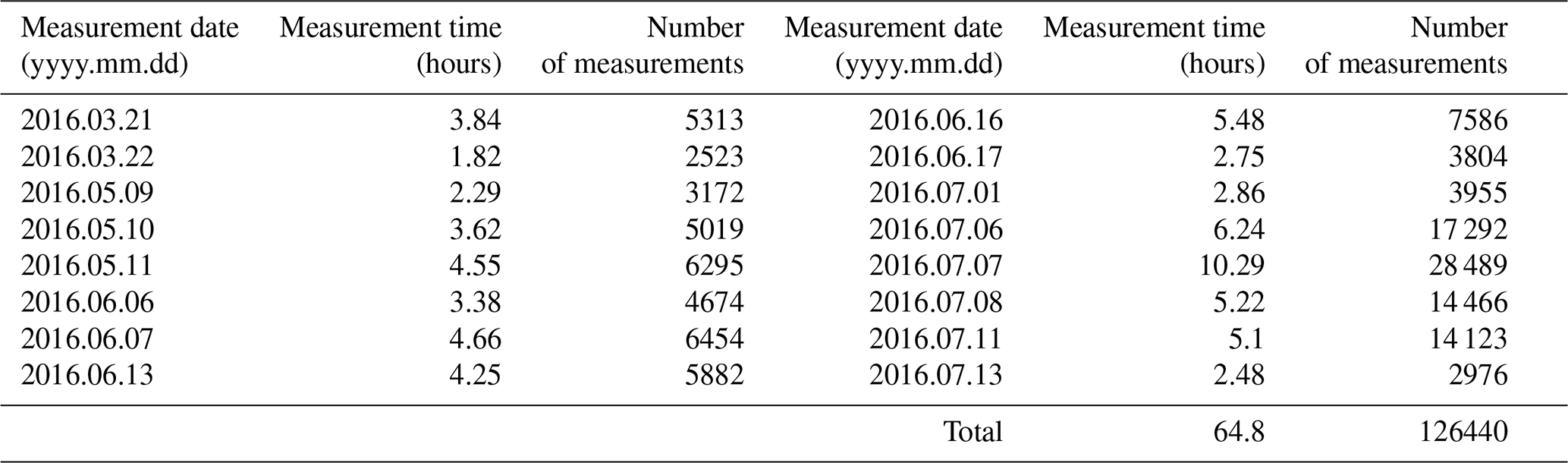
A CE DOAS and a CAPS instruments in two vehicles were used for on-street sampling of traffic emissions. The sampling inlets were located at the front right window of each vehicle at 1.5 m height. For measurements in Munich's city park (English Garden), we used a bike trailer. The measurements were performed on two days in March, three days in May, five days in June and six days in July 2016 to cover a large part of the urban area in Munich. Table 1 shows the dates, measurement times and number of measurements for all measurement days. The sample resolutions of the CE DOAS and the CAPS were both adjusted to 2 s during the mobile measurements. The measurements were performed on varying routes during daytime to cover the entire city center area. All measurements were spatially averaged to a high-resolution grid of 20 m × 20 m. This resolution has been chosen according to an average driving speed of 40–50 km h⁻¹ and the measurement sampling time of 2 s, so that at least one measurement value per drive-by falls into each grid box. All measurements from different drives and different days are averaged for each grid cell after diurnal cycle normalization.

Table 1 Overview of the measurement days, time and number of measurements.

The CE DOAS is composed of an air sampling system, an optical resonator with two highly reflective mirrors, a blue LED light source and a spectrometer (Platt et al., 2009). For the spectral retrieval in the wavelength range 435.6 to 455.1 nm, we used DOASIS (Kraus, 2005). The NO₂ reference absorption cross is from Vandaele et al. (2002), O₄ from Hermans et al. (1999), H₂O from Rothman et al. (2003) and CHOCHO (glyoxal) from Volkamer et al. (2005).

The CAPS measurement technique is closely related to cavity ring-down laser absorption spectroscopy (CRDS), which determines the concentration of trace gases from the decay rate of the light source in the optical resonator (Ball and Jones, 2003; Brown et al., 2002; Berden et al., 2000; Engeln et al., 1996). CRDS is a laser-based system, while CAPS uses an incoherent light source (a blue LED) that is well matched to the NO₂ absorption band. The CAPS NO₂ system mainly consists of a blue LED, a measurement chamber with two highly reflective mirrors centered at 450 nm and a vacuum photodiode detector. It estimates the NO₂ concentration by directly measuring the optical absorption of NO₂ at the 450 nm wavelength within the electromagnetic spectrum. The light appears as a distorted waveform after passing through two mirrors and the measurement cell, which is characterized by a phase shift that is determined by demodulation techniques in comparison to the initial LED light modulation. The phase shift is proportional to the absorbance of the light by the presence of NO₂. The concentration of NO₂ can be derived by measuring the amount of the phase shift. The detailed principles of the CAPS system are demonstrated in Kebabian et al. (2005b, 2008).

2.2 Long-path (LP) DOAS observations

Three LP DOAS instruments were installed on the roof of the MIM. The measurement setups are displayed in Fig. 1. The measurement system started operation in December 2015 with a total absorption path of 3828 m across the English Garden to a retroreflector array located on the rooftop of the Hilton hotel building at ∼ 48 m height. In January 2017 another absorption path of 1142 m was installed covering three blocks around the university area to a retroreflector at the St. Ludwig church in Munich at ∼ 40 m above ground. Since July 2015 a retroreflector has also been installed at the roof of the N5 building of the Technical University of Munich (TUM) at ∼ 28 m height, allowing an absorption path of 828 m. From July 2016 to August 2017 a path of 816 m to the roof of the building of the physics department of LMU at ∼ 24 m height was operational as well. For the long-term average diurnal cycle calculation described in Sect. 3.1.1 all available data from all measurement paths were used. LP DOAS measurements of light paths towards to the Hilton hotel, TUM and the LMU physics department were used to normalize the mobile measurements regarding the diurnal cycle. The measurement paths cover the university campus, the public park, residential areas and areas with heavy traffic. The instrumental background was corrected by subtracting the LED reference spectra, including dark current, offset and background, from each measured spectrum.

Figure 1 Map of Munich city center and four optical paths of three LP DOAS instruments. Map data © Google Maps.

A measurement sequence starts by taking a LED reference spectra using a shortcut system consisting of a diffuser plate in front of the y fiber and an exposure time of 10 s. Then a shutter is used to block the LED for measuring the atmospheric background spectrum for 1 s. Afterwards, the atmospheric spectrum with a maximum of 10 scans is taken. Each scan of a spectrum has a peak intensity of about 60 %–80 % saturation of the detector and typically requires 60–1000 ms, depending on the visibility and instrument setup. The total sampling time (the product of the number of scans and exposure time for each scan) was limited to 60 s. A full measurement sequence took between 30 and 90 s, depending on visibility conditions.

2.3 Local air quality monitoring network

The Bavarian LfU is operating five monitoring stations: three roadside stations at Landshuter Allee, Stachus and Lothstraße (locations of the three stations are also presented in Fig. 4c), and two ambient stations in Allach and Johanneskirchen. In these stations the air pollutants NO, NO₂, CO, O₃, PM_2.5, and PM₁₀ and in addition meteorological parameters such as relative humidity and temperature are measured. In this study we concentrated on the NO and NO₂ concentrations that are continuously monitored using an in situ CL NO_x analyzer (HORIBA APNA-370) (LfU, 2019).

3 Results and discussion

3.1 NO₂ concentration maps constructed using mobile measurements

The mobile measurement data can be used to create a map showing the city-wide distribution of air quality using NO₂ concentrations as a general indicator (Fig. 4). As a first test, we compared the averaged measurement values within a 10 km radius around the three governmental monitoring stations at Landshuter Allee, Lothstraße, and Stachus and obtained an averaged concentration of 93 µg m⁻³ for the mobile measurements and 48 µg m⁻³ for the three stations for the campaign days in June and July 2016. The large difference can be explained by looking at the criteria for the location of monitoring sites set by the European Union: the recommended measurement height is between 1.5 and 4 m; maximum distance to the street is 10 m and at a minimum distance to the next crossroad of 25 m (Commission, 2008). Most monitoring stations have the inlet positioned at 4 m height. The mobile measurement data, however, include the significantly increased concentrations at crossroads, tunnel exits and other pollution hot spots. In addition, the height of the measurement inlets differs by 2.5 m between the mobile measurements and the governmental monitoring stations, which also influences the comparison. In order to determine how representative point measurements are for the city-wide air quality, we analyzed the correlation between point measurements and the distribution captured by mobile measurements, between point and path-averaging measurements, as well as between path-averaging and satellite measurements. Since the spatial distribution can not be captured instantaneously, an algorithm to normalize for the diurnal variation is needed in order to create a consistent map representing only the spatial variability of daily average concentrations instead of temporal influences.

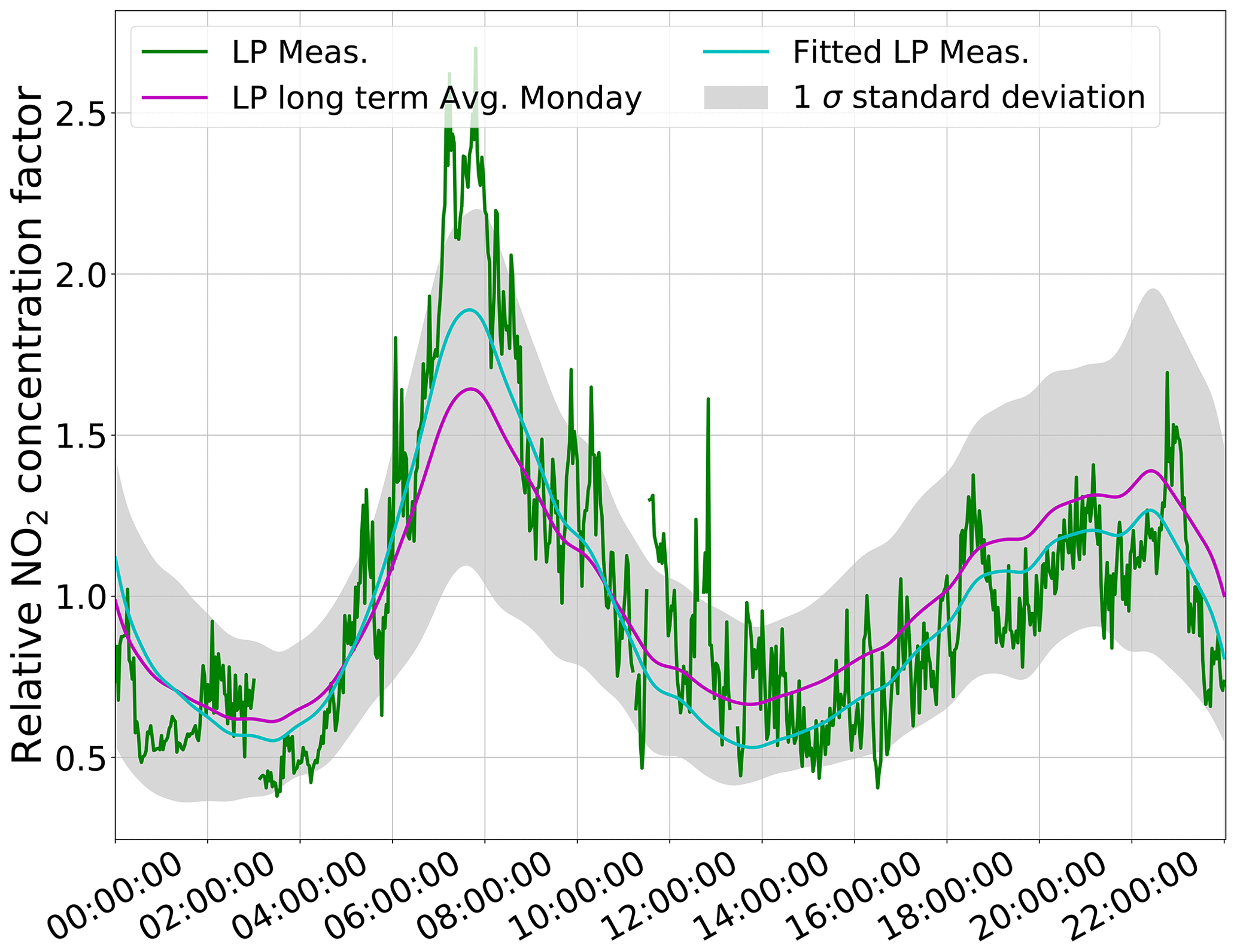
Figure 2 Normalization curve used to correct mobile measurement data. The purple curve is the long-term average diurnal pattern for the day of the week of the measurement day (Monday in this example), which is fitted (scaling with the linearly time dependent factor and offset) to the measurement data of 13 June 2016 shown in green, excluding the data outside of the 2σ area shown in gray. The resulting cyan curve is used to remove the diurnal dependency of the mobile measurements data.

3.1.1 Normalization of the diurnal cycle

As a mobile survey cannot capture the concentrations at different locations simultaneously, and the NO₂ measurements are naturally influenced by daily variations such as changing boundary layer height or the diurnal cycle of the traffic amount, we use an algorithm to separate temporal and spatial patterns in the data set.

First, the algorithm normalizes the long time series of LP DOAS measurements of atmospheric NO₂ by dividing through the daily average NO₂ concentration of the same day. The mean concentration curves for each day of the week over a period of 2.5 years are calculated in order to obtain a relative diurnal NO₂ variation pattern (purple curve in Fig. 2). The normalized averaged diurnal NO₂ curve of the corresponding weekday is fitted (using an offset and a scaling with a linearly time dependent factor) to the normalized LP DOAS measurement of the corresponding day, coinciding with the mobile measurements. In order to remove the influence of outliers, NO₂ values outside of 2σ variation of the fitted curve are disregarded (cyan curve). Fig. 2 shows the fitting process for the normalization curve for one day of the measurement campaign. The other days show very similar characteristics with a significant peak in the morning and evening rush hours. Dividing the mobile measurement data by the curve data removes the diurnal dependencies and allows focusing on spatial pattern.

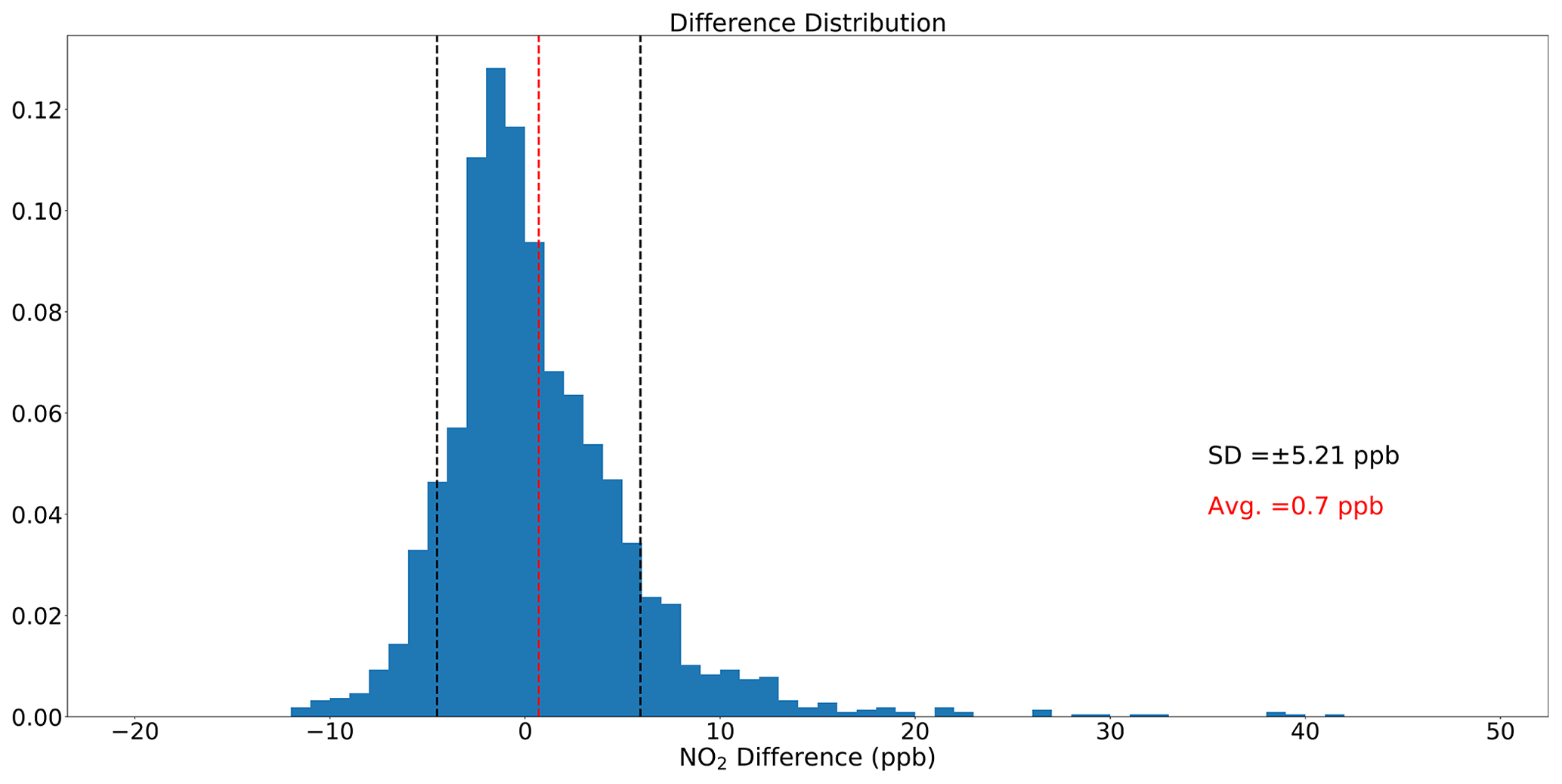
Figure 3 The distribution of the differences in between the inferred daily average concentrations and 24 h average concentrations measured by LfU stations. Bin width is 1 ppb. Evaluated stations including Allach, Johanneskirchen and Lothstraße.

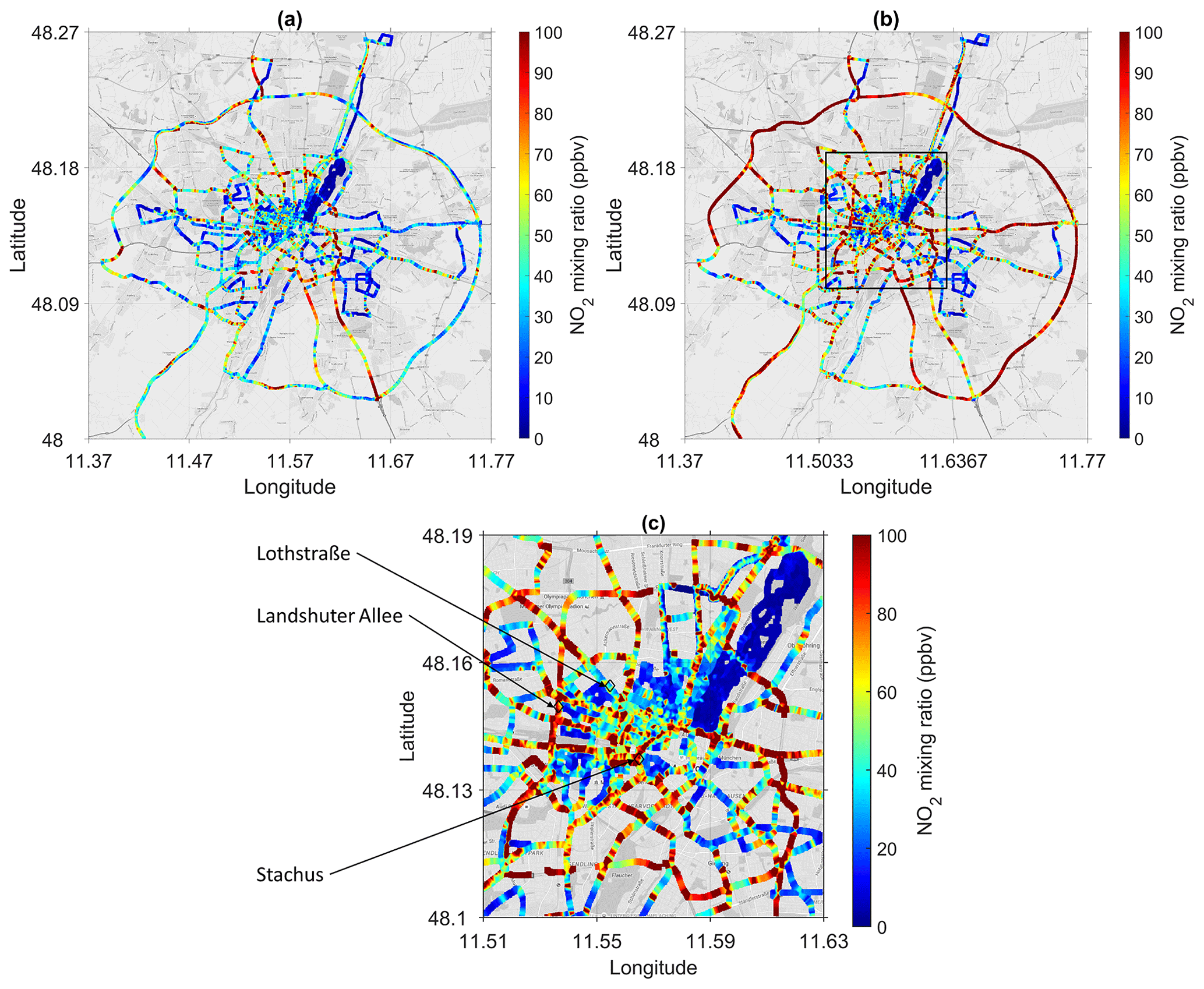
Figure 4 (a) CE DOAS and CAPS mobile measurements of NO₂ in Munich in 2016. (b) Normalized spatial distribution of NO₂ using coinciding LP DOAS data to remove the diurnal dependencies. (c) Close-up of the city center. The three black diamonds in panel (c) are the locations of the governmental monitoring stations (Landshuter Allee, Lothstraße, Stachus). The area at the top right with very low concentrations represents the city park English Garden. Map data © Google Maps.

The corresponding stationary measurements from three LfU stations on mobile measurement days were used to evaluate the accuracy of the normalization algorithm. The inferred daily average concentration for each stationary measurement was retrieved based on the fitted LP DOAS normalization curve and then compared with the corresponding 24 h average concentration measured by the same station. The distribution of the concentration differences is shown in Fig. 3. The averaged difference is 0.7 ppb with 1σ uncertainty of 5.21 ppb. The inferred daily averages compared to the actual average concentrations at the stations Landshuter Allee and Stachus differ more because due to frequent traffic jams and stop-and-go traffic they show a different diurnal cycle. Overall, the normalization algorithm effectively separated the temporal and spatial influence for most mobile measurement locations.

Table 2 Percentage of measured concentrations exceeding the WHO AQG 1 h guideline and its corrected on-road level thresholds for both temporal and spatial coverage. The values are broken down for before and after the normalization of the data according to diurnal patterns and also calculated for WHO guideline values adjusted for the different measurement height and distance to the street.

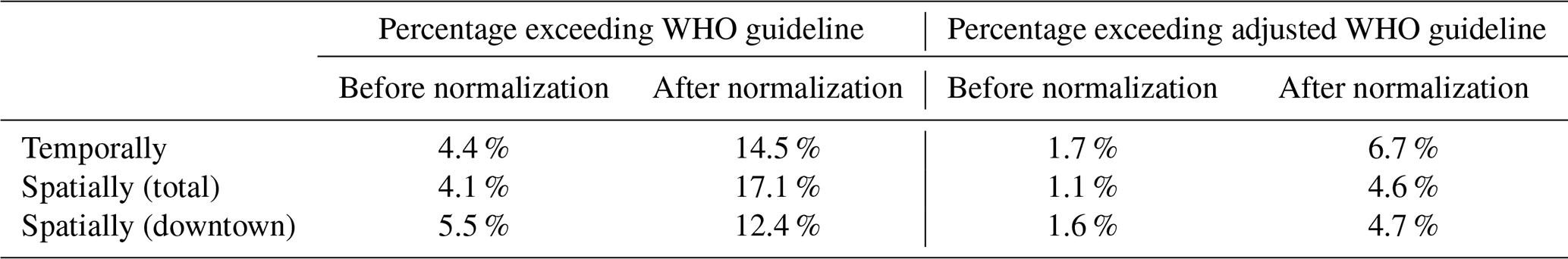
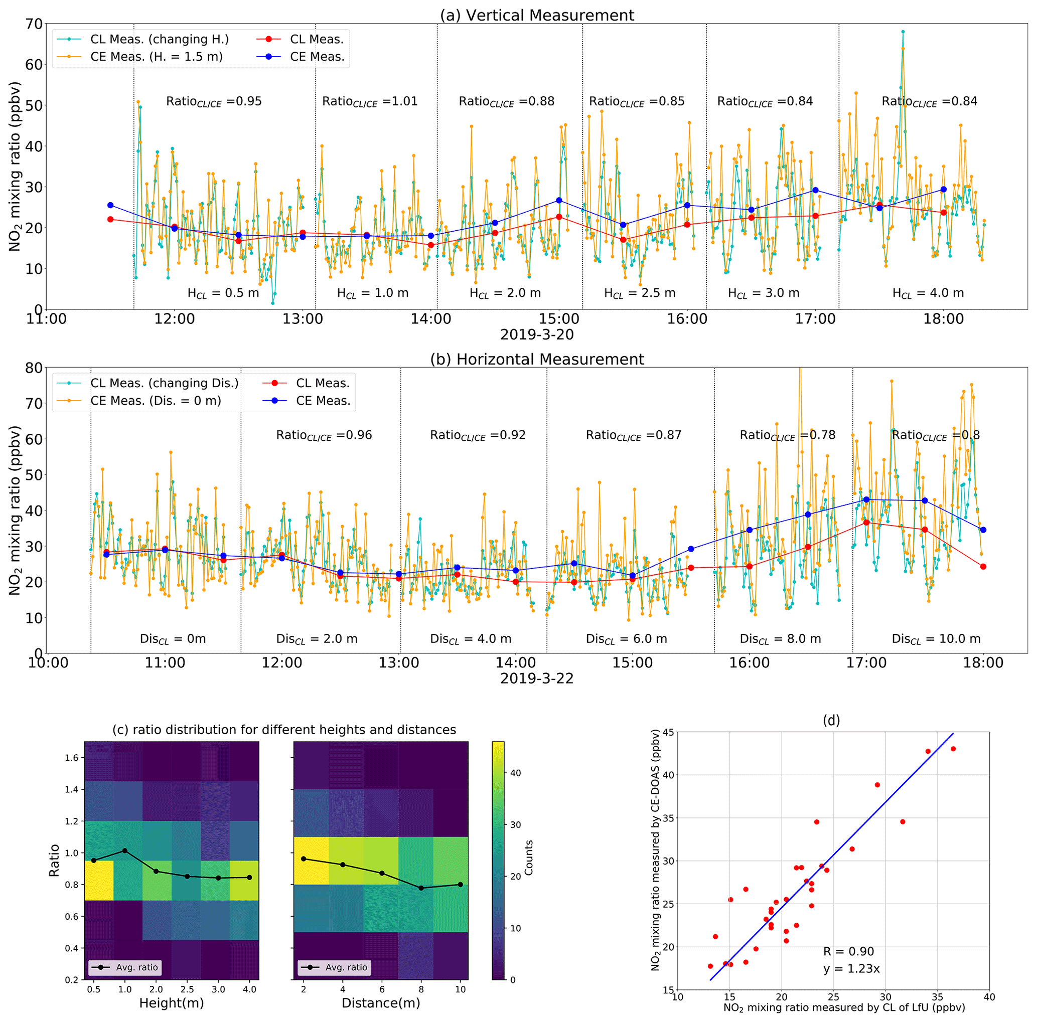
Figure 5 NO₂ measurements at Karlsplatz (Stachus), Munich, with different heights above ground (a) and distances to the main street (b). The ratio between 1 min averaged CE DOAS and coinciding CL measurements were calculated individually for the different heights and distances. Half-hour averaged CE DOAS measurements (blue curve) were compared with the corresponding CL measurements (red curve). Averaged ratios for different heights and distances (as defined in panel a) are shown in panel (c); CE DOAS measurements at 1.5 m were averaged to 30 min intervals and compared with the half-hourly data of the governmental monitoring station at 4 m shown in panel (d).

3.1.2 Spatial distribution of NO₂ in the city of Munich

The measured concentrations during the campaign were spatially averaged to a high-resolution grid of 20 m × 20 m (Fig. 4a). Most of these measurements are distributed on major roads, including city, urban ring road, suburbs, rural areas and highways. Relatively high NO₂ pollution could be observed on motorways and busy urban roads. A difference between main roads and adjoining side roads of up to a factor of 5 can be observed. A total of 4.4 % of the on-road measurements exceeded the WHO 1 h guideline value of 200 µg m${}^{-\mathrm{3}}\approx$ 106 ppb (depending on temperature, here the appropriate conversion factor at 25 ^∘C and 1013 hPa are used), corresponding to 4.1 % of the area covered. Note that WHO reference concentration refers to 1 h average values, whereas we measure at each location for a few seconds. We use this comparison to show how often this threshold would be exceeded if the drive-by measurement were representative local respective situations. High NO₂ values over motorways were mainly due to the emission of heavy duty diesel vehicles; i.e., a significant increase could be observed when we were driving behind trucks and buses. In the city center traffic congestion and the street canyon effect (Rakowska et al., 2014) can be the main cause of elevated on-road NO₂ levels. Zhu et al. (2018) showed in a study in Hong Kong that average pollution exposure increases by 14.5 % when stopping at a traffic light compared to fluent traffic. Other studies showed as well that the distribution of pollutants is mainly impacted by traffic flow patterns (Fu et al., 2017; Rakowska et al., 2014; Huan and Kebin, 2012; Kaur et al., 2007; Westerdahl et al., 2005). The normalization using coinciding LP DOAS measurement removes the diurnal dependency but leaves the traffic flow dependency in the data, because it contributes to the city-wide air quality. The normalized on-road NO₂ map shown in Fig. 4b represents daily average values for all locations. After normalization, there exist some regions where NO₂ concentrations are consistently higher, while in other areas the normalized concentrations are lower than the original measurements. This behavior can be explained by the time of the day when the measurements were taken: when we measured during the rush hour, the measurements were higher, while the measurements during noon are lower than the daily average. The normalization procedure increased the occurrences of WHO 1 h guideline exceedances to 14.5 % of the on-road measurements, corresponding to 17.1 % of the total area (including motorways) and 15.7 % of the area in the city center. However, the thresholds in WHO AQG are based on studies involving monitoring station data which are not measuring directly on the street. Taking the vertical and horizontal dilution factors (see Fig. 5, the factor 0.84 for 4 m height and 0.87 for 6 m distance) into account, we extrapolate the WHO AQG 1 h threshold value of 200 µg m⁻³ to the on-road level with the value of 273.7 µg m${}^{-\mathrm{3}}\approx \mathrm{145.6}$ ppb (200 µg m${}^{-\mathrm{3}}/\mathrm{0.84}/\mathrm{0.87}$)), and we then also calculated the frequency of exceedances (see Table 2).

It can be seen that, especially in the downtown area (Fig. 4c), the values after the normalization are noticeably higher than before. This can be explained as we tried to avoid the rush hours, i.e., traffic jams, for performing the measurements. Therefore, the measured NO₂ level is often lower in comparison to the day average. The area with significantly lower concentrations seen in Fig. 4 is the city park (English Garden) with no vehicle emissions and where plants could provide deposition areas for O₃, NO_x and particles (Chaparro-Suarez et al., 2011; Wesely and Hicks, 2000).

3.2 Comparison of NO₂ concentrations at different heights and distances from the street

In order to investigate the diffusion effects of emitted NO₂ molecules in both vertical and horizontal directions, measurements were conducted over two days (20 and 22 March 2019) using CE DOAS and CL instruments at Stachus, Munich, next to the governmental monitoring station. Since we used two different measurement techniques, the first step was to check the instrument for consistency. Side-by-side measurements next to the street (same height and distance to the street in Fig. 5) were used to analyze differences. We found the CL NO₂ to be 2 % higher, possibly due to sensitivities of the molybdenum oxide converters to NO_y species (see Villena et al., 2012; Dunlea et al., 2007). We corrected the CL measurement data in order to remove those interferences.

Both instruments were set up next to the governmental monitoring station at Stachus, which is at a height of 4 m and has a 30 min time resolution. The CE DOAS was set up next to the street and measured at a fixed height of 1.5 m above the ground, while the CL instrument measured NO₂ at multiple heights above the ground (from 0.5 to 4 m) and at different distances from the side of the street (from 2 to 10 m). The temporal resolution for both instruments was set to 5 s. All measurements are shown in Fig. 5a for the different measurement heights and Fig. 5b for the different distances to the side of the street. Figure 5c shows the distribution of the ratios, and it can clearly be seen that the average concentrations decrease with height and distance. Another mobile measurement study by Apte et al. (2017) also demonstrates the distance-decay characteristic of the urban spatial distribution of NO, NO₂ and black carbon but on larger scales. More relevant theoretical decay research can be found in Choi et al. (2012, 2014). Figure 5d shows a two-day comparison between the 30 min average NO₂ concentrations measured with our CE DOAS at a height of 1.5 m with the CL instrument data of the governmental monitoring station at a height of 4 m. The regression plot shows a ratio of 1.23 between the measurements at 1.5 and 4 m height. In addition, the side-by-side measurement derives a factor of 0.84 with a standard deviation of 0.20, so most ratios vary from 37 % decrease with increasing height (factor $\mathrm{0.84}-\mathrm{0.20}=\mathrm{0.64}$) to 5 % increase (factor $\mathrm{0.84}+\mathrm{0.20}=\mathrm{1.04}$). Additional roadside measurements regarding the comparison between the 1.5 and 4 m measurement height were conducted at roadside next to the MIM building and the LfU station of Landshuter Allee on several different days during different seasons and derived a similar result. Since the inlet height for our mobile measurements is 1.5 m, we take this factor into account when comparing to monitoring station data. In addition, we analyzed how the uncertainty of the scaling factors (horizontal and vertical) contributes to the comparison with the WHO threshold shown in Table 2 and found that the percentage of exceedances can vary between 0.4 % and 23.8 %. It is because those dilution factors could vary, as they depend on factors in a small-scale environment, such as local meteorology, seasonality, local topography, urban morphology and traffic conditions. We do not assume that the scaling factors can be applied to all our mobile measurements but rather on average for our statistical analysis. For further distance-decay studies, it is essential to carry out more extensive and long-term side-by-side measurements to cover different measurement environments (such as different locations and seasons). In terms of distance to the street, measuring at the center of the street, like we did during the mobile measurements, and measuring at a distance of 6 m, which is approximately the distance of most monitoring stations to the middle of the street, the on-road measurements are 13 % higher with a standard deviation of 0.18 due to the observed diffusion effects. Those factors have to be kept in mind when comparing on-road measurements to monitoring station data or any other measurement data taken at different height levels and distances to the street. This leads to the conclusion that from the 48 % difference between the average concentrations of three monitoring stations (48 µg m⁻³) and the mobile measurements around the three stations (93 µg m⁻³), both averaged for the measurement campaign period, 27 % can be explained by the difference in inlet height and distance to the street, and the remaining 21 % is due to the fact that the monitoring stations are positioned away from pollution hot spots at crossroads according to WHO guidelines.

4 Summary and conclusions

Mobile road measurements using CE DOAS and CAPS instruments combined with an algorithm for correcting the diurnal cycle were used in order to generate a consistent pollution map of the street level NO₂ concentration in Munich. This map is not only used to identify pollution hot spots but also to figure out how representative the existing NO₂ point measurements are for the whole city. Elevated NO₂ levels can be observed mostly on motorways and busy city roads, due to the emission of heavy duty vehicles or heavy traffic volume. When averaging the mobile measurements around the monitoring stations, we derived an average NO₂ concentration of 93 µg m⁻³, whereas the three monitoring stations at the city center reported 48 µg m⁻³ on average for the same time, so 48 % lower values. Our analysis shows that the different measurement height can account for 16 % difference (factor 0.84), and the distance of the sample inlets to the center of the street, where the mobile measurements took place, explains the 13 % (factor 0.87) lower values. Accounting for these factors still leaves about 21 % that can be attributed to pollution hot spots like busy crossroads or tunnel exits. These hot spots are not covered by monitoring stations, which is intentionally done in order to make the long-term data less dependent on local events. Nevertheless, the differences observed in the presented study show that point measurements are likely not representative for the NO₂ concentration in the whole city. Most network measurement sites are not capturing the concentrations people are exposed to when walking or driving at the street level but are instead focusing on long-term trends. Our study illustrates the importance of combining different measurement techniques to capture spatial and temporal patterns within a city and derive concentration values that are representative for the air most people breathe in.

The pollution maps generated in this project provide valuable information for future urban planning and the design of control measures of environment pollution. Furthermore, it can provide guidelines for identifying representative locations for air pollution monitoring stations in a city. Additionally, the observed spatial distribution of NO₂ concentrations is also beneficial to the validation of chemical transport models and assessment studies of the impact of air pollution on human health.