the Creative Commons Attribution 4.0 License.
the Creative Commons Attribution 4.0 License.
 | 26 Apr 2019
Large-scale transport into the Arctic: the roles of the midlatitude jet and the Hadley Cell
Darryn W. Waugh
Clara Orbe
Guang Zeng
Olaf Morgenstern
Douglas E. Kinnison
Jean-Francois Lamarque
Simone Tilmes
David A. Plummer
Patrick Jöckel
Susan E. Strahan
Kane A. Stone
Robyn Schofield
Transport from the Northern Hemisphere (NH) midlatitudes to the Arctic plays a crucial role in determining the abundance of trace gases and aerosols that are important to Arctic climate via impacts on radiation and chemistry. Here we examine this transport using an idealized tracer with a fixed lifetime and predominantly midlatitude land-based sources in models participating in the Chemistry Climate Model Initiative (CCMI). We show that there is a 25 %–45 % difference in the Arctic concentrations of this tracer among the models. This spread is correlated with the spread in the location of the Pacific jet, as well as the spread in the location of the Hadley Cell (HC) edge, which varies consistently with jet latitude. Our results suggest that it is likely that the HC-related zonal-mean meridional transport rather than the jet-related eddy mixing is the major contributor to the inter-model spread in the transport of land-based tracers into the Arctic. Specifically, in models with a more northern jet, the HC generally extends further north and the tracer source region is mostly covered by surface southward flow associated with the lower branch of the HC, resulting in less efficient transport poleward to the Arctic. During boreal summer, there are poleward biases in jet location in free-running models, and these models likely underestimate the rate of transport into the Arctic. Models using specified dynamics do not have biases in the jet location, but do have biases in the surface meridional flow, which may result in differences in transport into the Arctic. In addition to the land-based tracer, the midlatitude-to-Arctic transport is further examined by another idealized tracer with zonally uniform sources. With equal sources from both land and ocean, the inter-model spread of this zonally uniform tracer is more related to variations in parameterized convection over oceans rather than variations in HC extent, particularly during boreal winter. This suggests that transport of land-based and oceanic tracers or aerosols towards the Arctic differs in pathways and therefore their corresponding inter-model variabilities result from different physical processes.
- Article
(9586 KB) - Full-text XML
-
Supplement
(569 KB) - BibTeX
- EndNote


The Arctic is characterized by the largest climate sensitivity with surface temperatures increasing much more rapidly than the global average in recent decades (IPCC, 2013). Trace gases and aerosols have been shown to be important for Arctic climate via their direct radiative influences and indirect effects on cloud properties (Garrett and Zhao, 2006; Lubin and Vogelmann, 2006; Coopman et al., 2018). Since the majority of these trace gases and aerosols originate over the Northern Hemisphere (NH) midlatitudes, where anthropogenic emissions are the largest (Bottenheim et al., 2004; Fisher et al., 2010; Kupiszewski et al., 2013), long-range transport from NH midlatitude source regions plays a crucial role in determining their Arctic distributions. Transport therefore has a remote impact on the Arctic climate as important as local forcings (Shindell, 2007). Shindell et al. (2008) further showed that the multi-model spread of simulated Arctic carbon monoxide (CO) and ozone (O3) concentrations is as large as the corresponding multi-model mean and this large multi-model spread may be related to large differences in long-range transport. It is therefore important that models correctly represent this transport.
Orbe et al. (2018) recently analyzed the transport in models participating in the Chemistry Climate Model Initiative (CCMI), and showed a large spread among the models. A 30 %–40 % difference of the multi-model mean is found in the Arctic concentrations of idealized tracers originating in the NH midlatitudes. Orbe et al. (2018) attributed much of these differences in transport into the Arctic to differences in midlatitude convective transport (primarily over the oceans) among the models, particularly during boreal winter. Specifically, they showed that, for tracers with zonally uniform sources over the NH midlatitudes, stronger convection over the oceans tends to enhance tracer concentrations in the upper troposphere and dilute tracer concentrations at the surface. While this enhances transport into the upper troposphere, it also weakens along-isentropic transport from the midlatitude surface into the Arctic middle troposphere, manifesting as negative correlations between midlatitude convection and Arctic tracer concentrations.
A limitation of the study of Orbe et al. (2018) is that the authors focused on idealized tracers with zonally uniform sources, and hence it is unclear whether their conclusions apply to more realistic tracers. Most chemical tracers of interest have strong zonal asymmetries in their source regions, with emissions primarily over midlatitude continents (e.g., tracers with anthropogenic emissions). These tracers may be less sensitive to differences in the simulated convection (which occurs predominantly over the oceans), and there may be less spread among the models in the transport of these tracers into the Arctic.
Here we revisit the issue of transport into the Arctic within the CCMI models, considering an idealized “CO5O” tracer. This tracer has realistic, zonally varying emissions corresponding to anthropogenic carbon monoxide (CO) emissions but with an idealized, fixed decay time of 50 d. We examine the transport of CO50, and also the “NH50” tracer (the same 50 d lifetime but with a zonally uniform boundary condition) considered by Orbe et al. (2018), into the Arctic within the CCMI models, and show that there is a spread in Arctic concentrations of both tracers among the models. This spread of CO50 is, however, not closely linked to differences in convective mass fluxes but is more likely due to differences in the midlatitude jet over the Pacific Ocean and in the mean meridional circulation.
Section 2 introduces the models, tracers, and dynamical metrics examined. Section 3 shows the multi-model mean tracer distribution followed by highlights on the multi-model spread of tracer concentrations over the Arctic. Section 4 focuses on examining the influences of the midlatitude jet on the poleward transport of tracers, in which we further explore the mechanisms. To further examine the role of tracer boundary condition and lifetime, Sect. 5 compares transport of CO50 (zonally asymmetric emissions) to the Arctic with another idealized tracer NH50 with zonally uniform sources as well as a realistic tracer, carbon monoxide (CO), with a temporally and spatially varying chemical lifetime. Conclusions and discussions are given in Sect. 6.
2.1 Models and experiments
This study analyzes simulation results from models participating in the Chemistry Climate Model Initiative (CCMI) phase 1 (Morgenstern et al., 2017). CCMI is a joint activity of the International Global Atmospheric Chemistry (IGAC) and Stratosphere-troposphere Processes And their Role in Climate (SPARC) projects that aims to better quantify stratospheric and tropospheric ozone and other important chemical species using state-of-the-art chemistry–climate models (Eyring et al., 2013). Here, we examine distributions of the idealized CO50 and NH50 tracers (see Sect. 2.2) from 15 chemistry–climate models (CCMs) and one chemistry-transport model (CTM) (Table 1). These models mostly overlap with those considered by Orbe et al. (2018), and we use the same model names. Several simulations analyzed by Orbe et al. (2018) are not used here because the CO50 tracer is either not included or incorrectly implemented in these simulations. As in Orbe et al. (2018), we focus on two types of hindcast reference simulations, namely the C1 simulation (i.e., referred to as REF-C1 in CCMI) and the C1SD simulation (i.e., REF-C1SD in CCMI). Both C1 and C1SD simulations were forced by observed sea surface temperatures (SSTs) and sea ice concentrations (SICs) from the UK Met Office HadISST1 data set (Rayner, 2003), but they differ in the source of meteorological fields. C1 simulations calculate the meteorological fields within the model, whereas C1SD simulations use (or relax towards) meteorological fields from meteorological reanalyses. The models used in this study differ widely in many respects, including the model resolution, dynamical core, physical parameterizations, and chemical schemes (Tables 1, 2 and Morgenstern et al., 2017).
Table 1Simulations analyzed in this studya and their corresponding selected period and horizontal and vertical configurations. Names of simulations follow those in Orbe et al. (2018). FD is finite difference; FV is finite volume; STL is spectral transform linear; STQ is spectral transform quadratic; TA is hybrid terrain-following altitude; TP is hybrid terrain-following pressure; P is pressure.
a SOCOL-C1, MOCAGE-CTM, and ULAQ-C1 also output CO50, but are neglected from this study because CO50 is incorrectly implemented in these simulations. b Negligible differences in climatology between these simulations and another two corresponding GEOS simulations averaged with the period of 01/2000–12/2009. c Simulations are based on the TA coordinates, but the meteorological fields have been particularly interpolated into the P coordinates with 31 levels.
Table 2Tracers and dynamical/thermodynamic variables of models analyzed in the study. u and v are the zonal wind and meridional wind; CMF is the convective mass flux by moist convection updraft. Available variables are marked by “×”. Variables of some simulations are scaled to make comparison of output variables commensurate between simulations and details are listed in table footnotes. (Re)analysis for specified dynamics in C1SD simulations is listed in the second to last column; otherwise the meteorology is free-running (FR) in C1 simulations. Moreover, meteorological fields are specified by nudging in most C1SD simulations, except GEOS-CTM uses CTM and GEOS-C1SD uses replay (a process involves reading in the analyzed field every 6 h and recomputing the analysis increment using the same assimilation methods that produce the MERRA-2 reanalysis; see replay details in Orbe et al., 2017a). Nudging timescales vary among different modeling centers, and WACCM is the only model that has two simulations with different nudging timescales (i.e., 50 h in WACCM C1SDV1 and 5 h in WACCM C1SDV2). The moist convection scheme is listed in the last column.
a There are only two levels below 800 hPa (i.e., 850
and 1000 hPa) for model output in P coordinates. Therefore, further
vertical interpolation is problematic near the surface
due to large
impacts of topography at 1000 hPa, and analyses on lower-troposphere v and
related diagnosis of the Hadley Cell exclude these simulations.
b Scaled by 1∕9.80665.
c Scaled by 100.
d Scaled by 0.001.
Fields analyzed in this study are listed in Table 2. We use monthly output from 2000 to 2009 for all CCMI simulations (except for GEOS-C1 and GEOS-C1SD; see Table 1), and calculate 10-year climatologies for northern winter and summer by averaging the months of December–January–February (DJF) and June–July–August (JJA), respectively. In addition, interpolation is applied from each simulation's vertical levels as in the archived output (isobaric, hybrid pressure, or hybrid altitude) to standard isobaric vertical coordinates consisting of 19 tropospheric levels (from 1000 to 100 hPa with a uniform spacing of 50 hPa) and four stratospheric levels (at 80, 50, 30, and 10 hPa). Analysis of individual models is performed using each model's native horizontal grid, but when forming multi-model mean fields, the model output is interpolated onto a standard 1∘ × 1∘ grid at every isobaric level after the interpolation to common levels noted above.
2.2 Tracers
To quantify the large-scale transport from the NH midlatitude land sources to the middle-troposphere Arctic, we examine the idealized CO50 tracer. The CO50 tracer has a flux boundary condition, corresponding to the annual mean value of anthropogenic emissions of CO for 2000, from the Hemispheric Transport of Air Pollution (HTAP) REanalysis of the TROpospheric chemical composition (RETRO) (Eyring et al., 2013), and a spatially uniform loss with a 50 d e-folding decay time. One exception is the EMAC models that use the annual cycle rather than the annual mean value of anthropogenic CO emissions for 2000. This results in higher CO50 concentrations during winter and lower concentrations during summer compared to the other models, which influences some results in this study but is unlikely to change any major conclusion (as we show in the remainder of the paper). There are strong zonal asymmetries in the CO50 emissions (white-dotted regions in Fig. 1), with the largest contributions from East and South Asia. Note that a similar 50 d CO-like tracer has also been used in many previous studies for diagnosing long-range transport, but in these previous studies the emissions included those from biomass burning (Shindell et al., 2008; Fang et al., 2011; Doherty et al., 2017).
Figure 1Ensemble mean of the horizontal distribution of CO50 concentration (shades, units: ppbv) at levels of (a, b) 850 hPa and (c, d) 500 hPa, and ensemble mean of the zonal-mean CO50 concentration cross sections (e, f) during (a, c, e) DJF and (b, d, f) JJA. In (a)–(d), horizontal winds (u, v) are overlaid as vectors, and regions of CO50 sources are highlighted by white stipples within which CO50 emission fluxes are larger than kg m−2 s−1. In (e) and (f), isentropic surfaces are overlaid as dark gray isopleths (units: K), the tropopause is marked as the bold dark gray curve, and regional convective mass flux (CMF) over East Asia (110–140∘ E) is denoted by white contours (units: 10−3 kg m−2 s−1).
We also compare the simulated CO50 to the NH50 idealized tracer. The NH50 also has a spatially uniform 50 d loss, but with a different boundary condition. The concentration of NH50 (χ50) in the bottom model level is specified as a fixed mixing ratio (i.e., 100 ppbv) over the NH midlatitude region (30–50∘ N, 180–180∘ W). Wu et al. (2018) have shown the spatial distribution of NH50, particularly its inter-hemispheric gradient, is strongly associated with the seasonal shift of the Intertropical Convergence Zone (ITCZ) and also likely the Southern Pacific Convergence Zone (SPCZ) over the oceans. As noted in Sect. 1, Orbe et al. (2018) further documented a wide spread of NH50 concentrations amongst CCMI models both over the Arctic and in the SH, and attributed this spread to the inter-model variation in low-level parameterized convection primarily over the oceans.
Last, to examine how well CO50 can represent real tracers with land sources, we compare it with carbon monoxide (CO) that undergoes the full chemistry (spatially and temporally varying) in the models. CO is removed from the troposphere primarily by reacting with the hydroxyl radical (OH) that yields a global mean annual mean lifetime of ∼2 months. However, as OH concentrations are much higher as well as for the temperature during summer, CO lifetime is much shorter in summer than that in winter. The emissions of CO generally resemble that of CO50, but it has additional sources from biomass burning, which features large emissions from forests in West Africa, South America all year round, and Siberia during summer. The latter is particularly important for the Arctic abundance of CO, and complicates comparisons with CO50.
For all the above tracers, we are particularly interested in their concentrations over the polar region in the middle and lower troposphere (70–90∘ N, 500–800 hPa) because it is the critical layer for realistic chemicals to exert direct radiative impacts and indirect radiative impacts via interaction with clouds.
2.3 Dynamical fields
As previous studies have indicated the importance of the midlatitude jet streams and associated storm tracks for tracer transport into the Arctic (e.g., Eckhardt et al., 2003), we also examine the relationship of the distributions of the above tracers with dynamical (meteorological) fields. In particular, we decompose the tracer transport into a zonally asymmetric component and a zonally symmetric component. The zonally asymmetric transport is associated with eddy mixing and we examine the relationship with the NH midlatitude jet. The zonally symmetric transport is associated with the zonal-mean flow advection and we examine the relationship with the Hadley Cell (HC) circulation.
For the midlatitude jet, we focus on the zonal wind u over the Pacific Ocean, as this plays an important role in the transport of CO50 away from the major source region over East Asia, and examine the variation in the latitude of the Pacific jet (ϕjet). This latitude is where the zonally (135∘ E–125∘ W) and vertically (500–800 hPa) averaged u maximizes in the midlatitudes (25–65∘ N). Note that the 500–800 hPa average corresponds to the middle and lower troposphere where the midlatitude jet can have a significant impact on tracer transport via wave breaking. To account for differences in model resolution, ϕjet is calculated as the location of the maximum of a quadratic function fitted to the zonally and vertically averaged u at its maximum grid point and the two points either side (Barnes and Polvani, 2013). ϕjet is calculated at every season of the integration and the wintertime and summertime climatologies of jet position are then derived for inter-model comparison.
For the HC we examine the 800–950 hPa averaged zonal-mean meridional wind that may be important for tracer transport near the surface source relating to the lower branch of HC, and calculate the latitude (ϕv=0) at which between 20 and 50∘ N. This latitude corresponds to the surface divergence zone separating the NH Hadley Cell and Ferrel Cell. Again, ϕv=0 is calculated seasonally, and winter and summer climatologies are compared between the models.
We first examine the multi-model mean (i.e., C1 and C1SD simulations combined) distributions of CO50, and then examine the spread among the models with a focus on distributions in the Arctic. The CCMI multi-model mean horizontal and vertical distributions of CO50 are shown in Fig. 1. In both the lower troposphere (850 hPa) and the middle troposphere (500 hPa), and for both seasons, there are higher concentrations of CO50 (χCO50) over the midlatitudes than over the Arctic, with large zonal asymmetries over the midlatitudes but not in the Arctic. The maxima of χCO50 over the midlatitudes highlight the primary source regions of CO50 in East Asia and South Asia, with χCO50 decreasing rapidly away from the source regions.
The meridional and vertical distribution of zonal-mean CO50 varies with season. During boreal winter, CO50 features a much stronger meridional transport near the surface in both the poleward and equatorward directions. The distribution of CO50 also generally follows the slope of isentropic surfaces, exhibiting stronger vertical transport north of the midlatitude CO50 source region and suppressed vertical transport in the south. During summer, χCO50 has a weak vertical tracer gradient and a secondary maximum at 200–300 hPa in the subtropics, indicating reduced meridional transport compared to winter. This secondary maximum in CO50 mixing ratio requires robust vertical transport with relatively slow chemical loss, which is likely due to the close proximity of the emissions to the strong continental convection underlying the summertime Asian monsoon anticyclone over the Tibetan Plateau (Park et al., 2007; Garny and Randel, 2013) (see Fig. S1 in the Supplement). A similar maximum within the Asian monsoon anticyclone region near the tropopause was observed by balloon sondes for particle surface area density of aerosols (Yu et al., 2017), as well as for CO in the upper troposphere over East Asia by flight measurements (Holloway et al., 2000; Palmer et al., 2003).
Figure 2(a, b) Latitudinal and (c, d) vertical variations in zonal-mean CO50 concentration χCO50 (units: ppbv) for each model during (a, c) DJF and (b, d) JJA. The corresponding ensemble means are depicted as the heavy gray lines. In (a) and (b), χCO50 values are averaged in the middle and lower troposphere (500–800 hPa); whereas in (c) and (d), χCO50 values are averaged over the Arctic (70–90∘ N). Note that C1 simulations are shown as solid lines while C1SD simulations are shown as dashed or dotted–dashed lines.
The spatial distribution of zonal-mean CO50 for each model is similar to that for the multi-model mean distribution discussed above. This is illustrated in Fig. 2, which shows the latitudinal variation in lower troposphere (500–800 hPa) and vertical profiles of Arctic (70–90∘ N) CO50. Although the latitudinal and vertical structures of CO50 concentrations are similar among the models, there is a large spread in the magnitude of CO50 tracer concentrations. The multi-model spread is the largest over the midlatitude source region, decreasing rapidly in the tropics south of the source region while remaining relatively large north of the source towards the Arctic for both seasons.
We will focus here on model differences in CO50 concentrations over the Arctic, and the poleward transport from NH midlatitudes. The differences in Arctic CO50 concentrations among the models peak around 400 hPa during winter and remain at a similar maximum for all levels below 400 hPa during summer. In the middle and lower troposphere, the range of χCO50 among the models decreases from ∼7 to 10 ppbv in winter to ∼5 ppbv in summer; this yields a 30 %–45 % wintertime fractional spread (i.e., the multi-model spread relative to the corresponding multi-model mean) and a 25 %–30 % summertime spread of Arctic χCO50. Note that χCO50 values in the EMAC models are biased due to the use of seasonally varying CO50 emissions, which manifest as higher χCO50 during winter and lower concentrations during summer. However, it is not possible to use a simple scaling on χCO50 to correct for this bias. if we assume no seasonality of CO50 emissions in the EMAC models (as the other CCMI models), we expect a lower Arctic χCO50 during winter and a higher Arctic χCO50 during summer; this would yield a smaller multi-model spread of Arctic χCO50 during winter and likely a larger range during summer.
The difference between pairs of simulations (and hence the ordering of simulations) is generally the same at all altitudes. For example, χCO50 in winter is smaller in ACCESS-C1 and NIWA-C1 than that in the EMAC simulations throughout most of the tropospheric column. This suggests that the above model spread of Arctic CO50 is related to a vertically consistent difference in the poleward transport rather than a tracer redistribution between different levels.
The large spread in CO50 concentration among the models is consistent with the wide spread reported by Orbe et al. (2017b, 2018) for idealized tracers with zonally uniform sources. Also, Figs. 2 and S2 show that the spread in CO50 among the C1SD simulations (dashed lines) is comparable to or even larger than the spread among the C1 simulations (solid lines). This is again consistent with the results of Orbe et al. (2017b, 2018), and provides further evidence that using specified dynamics simulations does not constrain climatological tropospheric transport any more than using free-running models.
Having shown a large model spread in the Arctic concentrations of CO50, we now examine possible causes for these differences. Shindell et al. (2008) suggested that the Arctic CO concentration in the middle troposphere is equally sensitive to changes in emissions over Europe, Asia, and North America. However, given the total amount of emissions from Asia (East Asia and South Asia; see Table 2 in Shindell et al., 2008) is ∼2–3 times larger than those from Europe and North America, we first examine processes that are associated with the transport of Asian pollutants.
4.1 Relationship with midlatitude convection
Orbe et al. (2018) showed that differences in convection among the models contribute to differences in tracer distributions. They showed that models with stronger midlatitude convection tend to have lower Arctic concentrations of the idealized NH5 tracer (this tracer has the same zonally symmetric boundary conditions as NH50 but with a shorter lifetime of 5 d), especially during northern winter. However, examination of CO50 shows a very weak relationship between the strength of the midlatitude convection and the Arctic χCO50 in both winter and summer (Fig. 3). The strength of convection is measured using the convective mass flux (CMF) in the low-level midlatitudes, which is the average of 800–950 hPa, 30–50∘ N, and 130–170∘ E for boreal winter focusing on convection over the west Pacific Ocean and 110–140∘ E for summer highlighting continental and maritime convection over East Asia, as in Orbe et al. (2018). The average zones overlap the strongest intensity and the largest inter-model variability of convection. Note that the χCO50–CMF relationship during winter is sensitive to which models are included in the correlation since simply excluding the ACCESS and NIWA models would produce a positive correlation whereas excluding the EMAC results would produce a negative correlation. The latter is more plausible given the fact that the Arctic χCO50 values are biased higher in the EMAC models during winter and a better negative χCO50–CMF correlation can be achieved if the Arctic χCO50 values in the EMAC models are lower. Despite the complications associated with using the EMAC model results, this large sensitivity to including or excluding a few models indicates that special care must be taken when interpreting correlations using only a limited number of CCMI models. Furthermore, there are a few models that have a similar heritage (e.g., ACCESS and NIWA, WACCM, and CAM) but such a similarity does not affect the robustness of the results presented in this study. In particular, we find that correlation coefficients calculated using only one of these similar pairs are essentially the same as those using all the models; further, there is no change in statistical significance with reduced degrees of freedom (see Table S1 in the Supplement). Hence, variations in CMF do not seem to be the primary cause of variations in transporting CO50 into the Arctic.
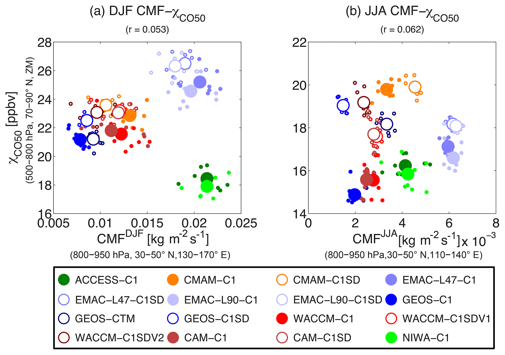
Figure 3Correlation between Arctic CO50 concentration χCO50 (units: ppbv) and low-level midlatitude CMF (units: kg m−2 s−1) in (a) DJF and (b) JJA. Arctic χCO50 is here the vertical average of 500–800 hPa and latitudinal average of 70–90∘ N, and zonal mean (ZM). CMF is here the vertical average of 800–950 hPa, latitudinal average of 30–50∘ N in both DJF and JJA, while the longitudinal average window differs between seasons, as DJF CMF highlights the robust convection over the western Pacific Ocean (130–170∘ E) whereas JJA CMF focuses on the maritime convection over East Asia (110–140∘ E) following Orbe et al. (2018). Large marks denote the 2000–2009 climatology (except GEOS-C1 and GEOS-C1SD) while small marks denote the corresponding interannual variations in each simulation. Results for C1 simulations are shown as filled circles while C1SD simulations are denoted by open circles. Results of the Pearson correlation coefficients based on climatological means are given in parentheses in the titles. If this correlation coefficient is significant (95 %), a corresponding linear regression is derived using the total least-square method (Petráš and Bednárová, 2010).
The absence of a strong correlation between Arctic CO50 and midlatitude convection may be largely due to the zonally asymmetric boundary condition of CO50, particularly in winter. With primary sources over land, CO50 tends to be less impacted by the variability of convection that maximizes over the oceans during winter. In summer, despite midlatitude convection being the strongest and also having the largest model spread over the land-based emission regions, the poleward transport of CO50 along isentropic surfaces is much weaker than that in winter (comparing Fig. 1f with Fig. 1e). Therefore, the Arctic CO50 concentration during summer is less connected to CO50 concentration over the midlatitude surface source regions and consequently shows a weaker correlation with the midlatitude convection.
4.2 Relationship with the midlatitude jet
Figure 1c and d suggest that, in addition to convection, the zonal winds u, especially over the northern Pacific Ocean, also play an important role in the transport of CO50 from its source regions. We therefore start by examining the structure of the midlatitude jet over the Pacific Ocean in the models. Figure 4 shows the latitudinal variation in lower-mid-tropospheric (500–800 hPa) zonal wind u averaged over the Pacific Ocean (135∘ E–125∘ W) for each model. In winter there is a similar latitudinal variation in u among the models. There is a variation in the magnitude of the peak winds but the latitude of this peak ϕjet varies by only a few degrees (∼35–40∘ N). The C1SD simulations, which use reanalysis winds, have very similar jet latitudes, with ϕjet∼36∘ N.
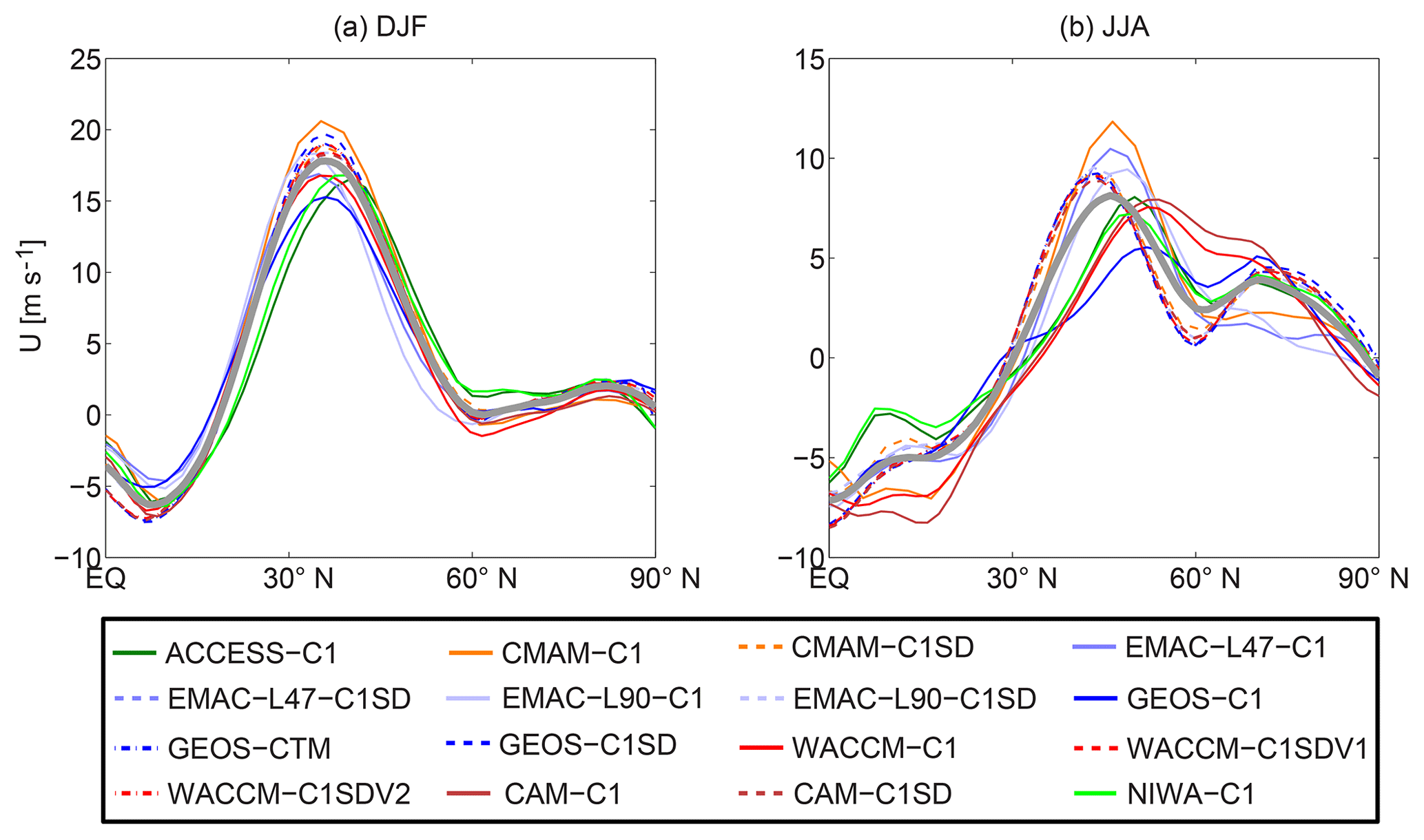
Figure 4Multi-model spread of latitudinal profile of zonal wind u vertically averaged between 500 and 800 hPa and longitudinally averaged over the Pacific Ocean (135∘ E–135∘ W) during (a) DJF and (b) JJA. C1 simulations are shown as solid lines while C1SD simulations are shown as either dashed or dotted–dashed lines. The corresponding ensemble means are depicted as the heavy gray lines.
However, in summer, there is a much larger variation among the models, not only in the magnitude and location of peak winds but also the latitudinal structure. ϕjet varies from ∼45 to 57∘ N, with the C1SD models at the lower end (ϕjet∼45∘ N). This implies that the latitude of the Pacific jet in C1 simulations is generally biased poleward of the reanalyses. A similar bias was found for models participating in phase 5 of the Coupled Model Intercomparison Project (CMIP5) (Barnes and Simpson, 2017). The variation in the summertime jet structure among the models is further illustrated in Fig. 5, which shows the 500–800 hPa averaged u during summer in each individual simulation. The C1SD simulations show strong winds across the Pacific with the jet axis tilting SW–NE. The C1 simulations show a much more varied structure, with many showing a more northern and more east–west jet that does not extend across the whole Pacific Ocean.

Figure 5Maps of 500–800 hPa averaged CO50 distribution (shades, units: ppbv) and the corresponding 500–800 hPa averaged u during JJA in each CCMI simulation. C1 simulations are shown in the top two rows while C1SD simulations are shown in the bottom two rows.
The summertime distribution of the 500–800 hPa average CO50 concentration is also shown in Fig. 5 (colors), and there appears to be a relationship between the midlatitude jet and the Arctic CO50 concentration. In general, lower χCO50 values over the Arctic are found in simulations with a more northern jet over the Pacific Ocean and higher χCO50 in simulations with a more southern jet (primarily the C1SD simulations). The correspondence between the latitude of the Pacific jet and the Arctic CO50 during summer is further quantified in Fig. 6a, which shows a scatter plot of Arctic χCO50 vs. ϕjet of the Pacific jet for summer. This shows that lower χCO50 is generally associated with a more northern ϕjet, with a clear negative correlation (−0.84) between the climatological-mean values for each model. This suggests that models with a more northern jet generally have weaker (slower) midlatitude-to-Arctic transport.
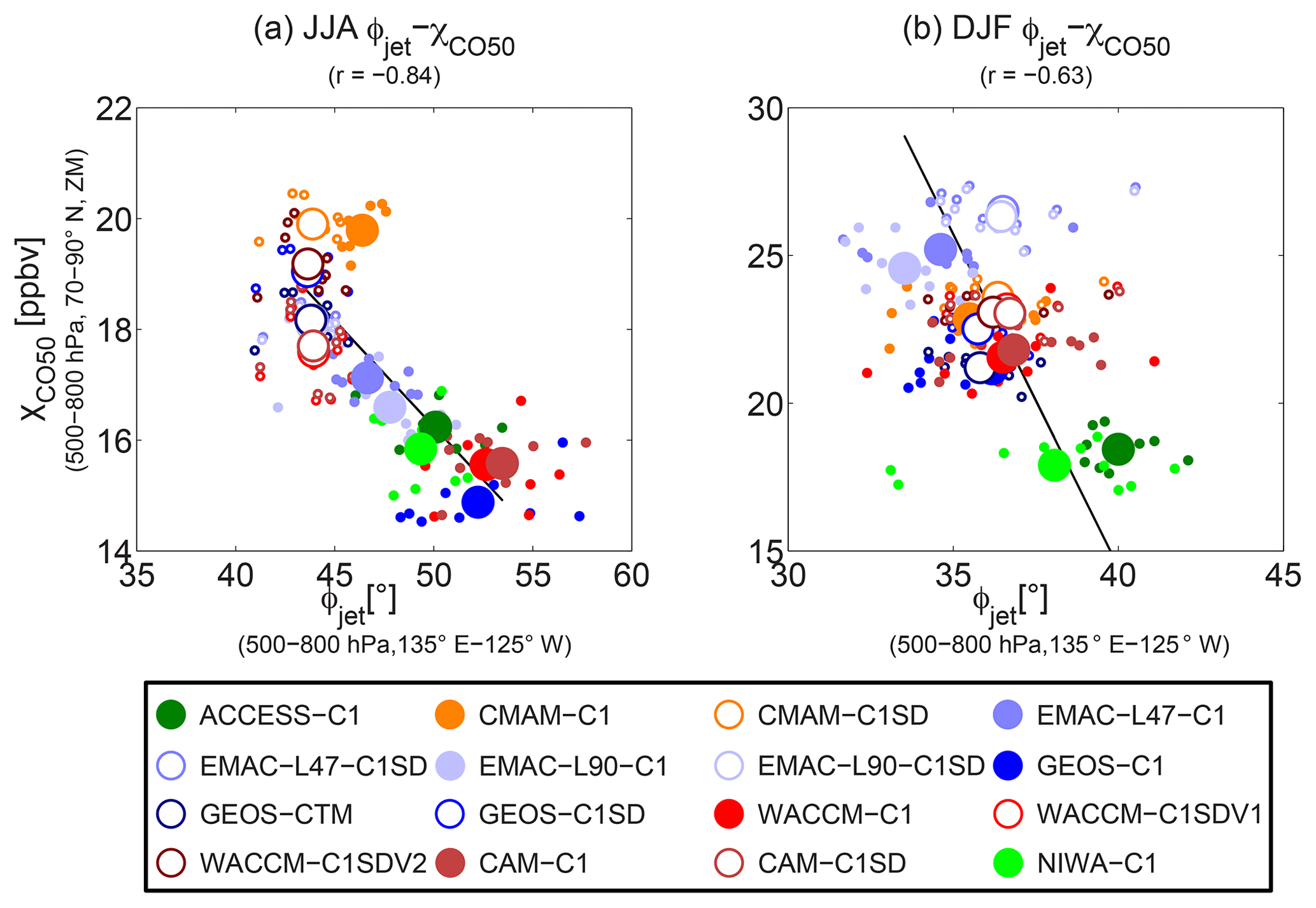
Figure 6Similar to Fig. 3, but for the correlation between Arctic χCO50 and latitudinal location of the NH midlatitude jet ϕjet over the Pacific Ocean (135∘ E–135∘ W) (Barnes and Polvani, 2013). Note that the sequence of displayed seasons switches with JJA in (a) and DJF in (b).
Repeating the above analysis for winter, we find the wintertime tracer transport from NH midlatitudes into the Arctic is also sensitive to the jet location, with negative correlations between χCO50 and ϕjet, as shown in Fig. 6b. This is somewhat surprising given the differences in jet structure among the models are much smaller in winter (see Fig. 4). Note that for both seasons, the ϕjet–χCO50 correlation is mostly achieved by C1 simulations with a similar or higher inter-model correlation among the C1 simulations comparing to those among all simulations (see Table S1). In C1SD simulations, u is well constrained and there is not much difference in jet location denoted by ϕjet. Therefore, spread of χCO50 among C1SD simulations cannot be explained by variations in ϕjet.
While there is a negative ϕjet–χCO50 correlation among the climatological means for each model, this does not hold for the interannual variations in individual models (small circles). One of the reasons may be that there are other aspects of the jet that can also impact the poleward transport of CO50, such as jet strength and jet structure (i.e., whether SW–NE tilted or zonal). These characteristics vary consistently with ϕjet for climatologies between models, but are less consistent at the interannual scale in individual models (not shown). Similar inconsistency occurs in ϕv=0 that quantifies the location of the mean meridional circulation, and as discussed next in Sect. 4.3.
4.3 Mechanisms
We now explore the underlying mechanisms for the above connection between the Pacific jet and transport into the Arctic. A strong jet with rapid zonal flow at its center can act as a barrier to meridional transport (e.g., Bowman and Carrie, 2002), but there can also be intensive transport on the flanks of the jet due to Rossby wave breaking (RWB) (e.g., Haynes and Shuckburgh, 2000). This RWB on the edge of the jets may explain the connection between jet location and transport into the Arctic. As shown by the schematics in Fig. 7, when the Pacific jet is in a more northern position (e.g., summertime jets in C1 simulations as shown in Fig. 5) the source region of CO50 is on the equatorward flank of the jet and the anticyclonic RWB occurring here transports CO50 equatorward and blocks transport to the Arctic. In contrast, when the Pacific jet has a more southern position and its western end tilts more southward (e.g., summertime jets in C1SD simulations), a fraction of the CO50 source region overlaps the poleward flank of the jet and the cyclonic RWB occurring there transports CO50 to higher latitudes and the Arctic. In other words, differences in the Arctic χCO50 between models with different jet locations could be due to differences in the meridional eddy transport caused by RWB.

Figure 7Schematics of mechanisms illustrating dynamic influences on the NH midlatitude-to-Arctic transport for the midlatitude jet situated more southern in (a) and more northern in (b). When jet location ϕjet and meridional flow switching point ϕv=0 are more southern, cyclonic wave breaking (CWB) along the poleward flank of the jet and northward surface meridional flow (green arrow) result in high tracer concentrations in the high latitudes. In contrast, when ϕjet and ϕv=0 are more northern, anticyclonic wave breaking (AWB) along the equatorward flank of the jet and southward surface meridional flow (blue arrow) result in low tracer concentrations over the Arctic. Tracer sources in the NH midlatitudes are denoted by the gray shades, isentropic surfaces are depicted as dashed lines, and red and blue triangles mark the latitude of ϕjet and ϕv=0, respectively.
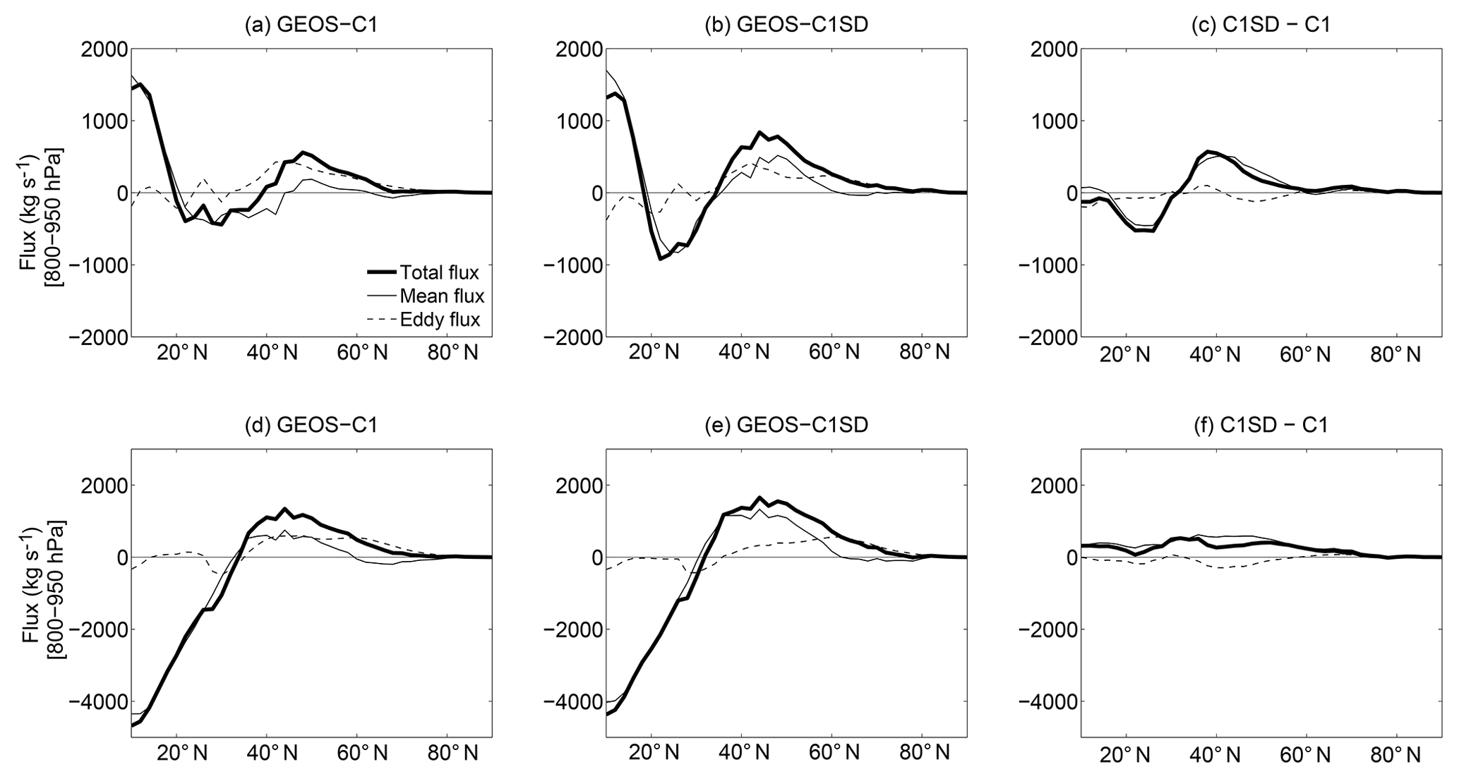
Figure 8Tracer flux diagnostics showing the total flux (heavy), zonal-mean flux (light, solid), and eddy flux (light, dashed) of CO50 (vertically integrated from 800 to 950 hPa; positive means northward; units: kg s−1) in (a) GEOS-C1, (b) GEOS-C1SD, and (c) the difference GEOS-C1SD–GEOS-C1 during summer. Panels (d), (e), and (f) are similar to (a), (b), and (c) but during winter. Results are based on the daily GEOS model output.
One approach to examine whether transport caused by RWB is the cause of differences in the transport into the Arctic is to decompose the tracer flux into zonal-mean and eddy components, i.e.,
where denotes the Eulerian zonal mean, ′ is the corresponding departure from the zonal mean, is the total flux, is the zonal-mean component, and is the eddy component. The meridional fluxes are further vertically integrated to yield the corresponding tracer mass flow rate across each latitude, i.e., the vertically integrated flux is
where F is the total, mean, or eddy flux, and rM is the ratio of molecular mass weight between CO (28 g mol−1) and dry air (28.97 g mol−1). ϕ is latitude, p is pressure, a is the Earth's radius of 6370 km, g=9.8 kg m s−2 is the gravity of Earth, and p1 and p2 are the upper and lower bounds for the vertical integral. Given that the tracer mass flux decays exponentially with altitude, the vertically integrated flux throughout the full tropospheric column is mostly captured by fluxes in the lower troposphere (Fig. S3c, d). Therefore, p1 and p2 are chosen as 800 and 950 hPa, respectively, to be consistent with the vertical examining region of CMF in low levels. Positive flux is defined as northward transport while negative flux corresponds to transport to the south.
A substantial contribution of the eddy flux comes from synoptic eddies, and to calculate this flux requires v and χCO50 at a higher frequency than the monthly-mean output available from the CCMI archive. However, we have access to daily output from GEOS-C1 and GEOS-C1SD simulations from 1990 to 1994, which can be used to examine the relative roles of mean and eddy fluxes in the meridional transport. As the Arctic χCO50 in GEOS-C1 is much lower than that in GEOS-C1SD (with the difference being almost the largest among CCMI simulations in summer; see Fig. 6), comparison of the fluxes between these simulations can test whether differences in eddy transport are the causes of differences in Arctic CO50 concentrations.
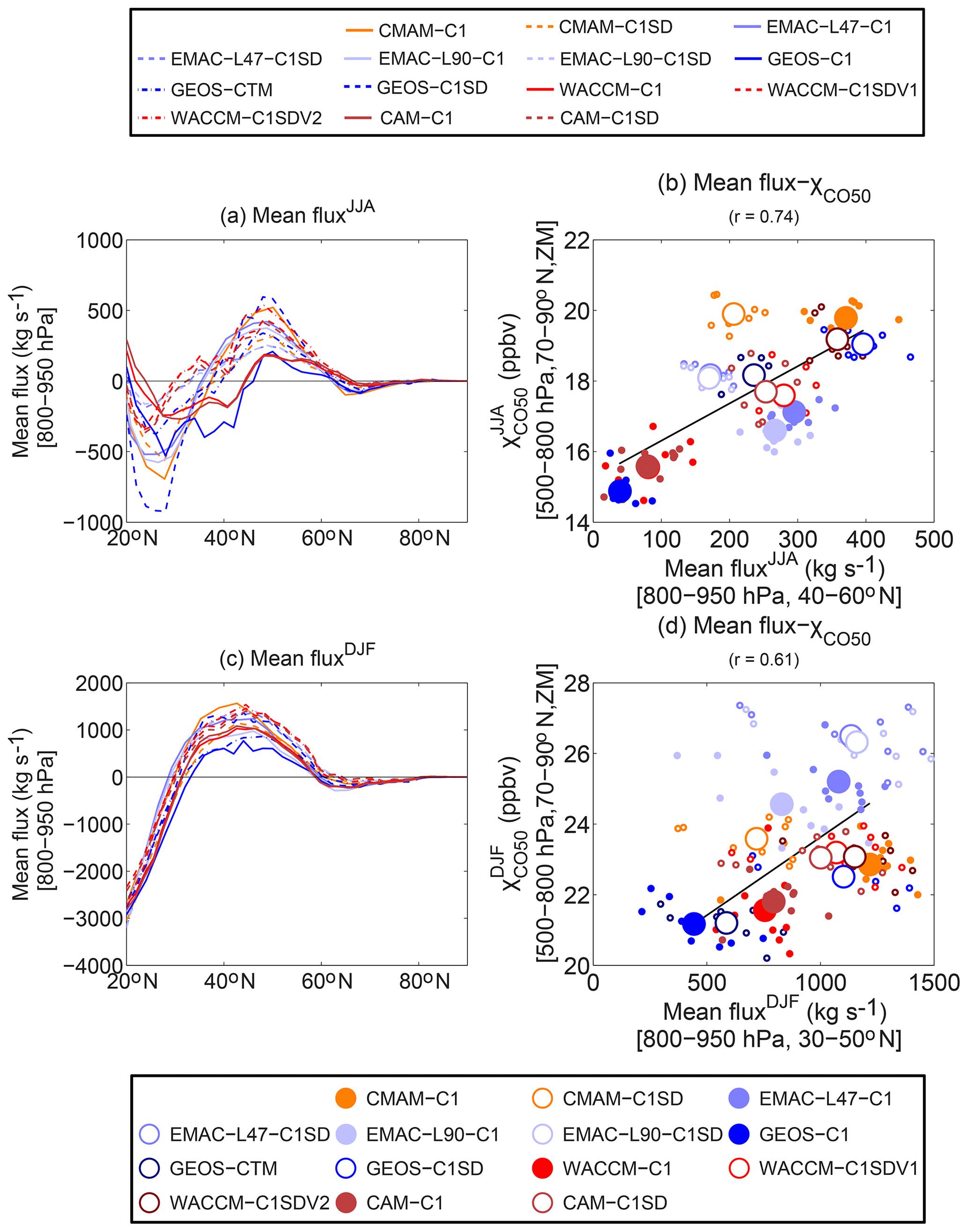
Figure 9Approximated zonal-mean flux using monthly output: (a, c) latitudinal profile of (units: kg s−1); (b, d) correlation between the zonal-mean flux (vertical average of 800–950 hPa, latitudinal average of 40–60∘ N during JJA and 30–50∘ N during DJF) and the Arctic CO50 concentration (vertical average of 500–800 hPa, latitudinal average of 70–90∘ N, and zonal mean (ZM), units: ppbv), during JJA in (a) and (b) and during DJF in (c) and (d).
The flux diagnostics for CO50 meridional transport in the two GEOS simulations are shown in Fig. 8. During summer, there is an equatorward transport of CO50 in the subtropics and a poleward transport in the extratropics in both simulations (bold curves in Fig. 8a, b). The latitude separating the equatorward transport from the poleward transport shifts from ∼40∘ N in GEOS-C1 to ∼34∘ N in GEOS-C1SD. Given that CO50 is largely emitted from East Asia and South Asia over 20–40∘ N, most of the CO50 source region is characterized by equatorward transport in GEOS-C1 but a significant fraction of the CO50 source stretches into the zone of poleward transport in GOES-C1SD. This yields a much larger poleward total flux over the midlatitudes in GOES-C1SD than that in GEOS-C1 (see Fig. 8c) consistent with a higher summertime Arctic χCO50 in GEOS-C1SD than that in GEOS-C1. Examination of the zonal-mean component and eddy fluxes shows that differences in the total fluxes are dominated by the zonal mean and not the eddy component (Fig. 8c). During winter, the latitude that separates the equatorward transport from poleward transport in GEOS-C1SD (∼36∘ N) is only slightly south of that in GEOS-C1 (∼38∘ N) (Fig. 8d, e). However, the total tracer flux of CO50 features a much larger poleward transport over the midlatitudes in GEOS-C1SD than that in GEOS-C1, and this large difference is again primarily due to difference in the zonal-mean fluxes.
The above analysis of tracer fluxes in GEOS-C1 and GEOS-C1SD contradicts our original speculation that the difference in Arctic χCO50 is due to the jet-associated RWB (and eddy transport). Instead, it indicates that differences in the zonal-mean component dominate, which is linked to transport by the mean meridional circulation. We are unable to perform this tracer flux decomposition in all CCMI simulations due to a lack of daily data. However, we can approximate the zonal-mean components of tracer flux using monthly-mean fields as the zonal-mean flux is largely associated with the slowly varying mean meridional circulation. We have confirmed that the zonal-mean flux calculated using monthly output differs only slightly from the one using daily output in both GEOS-C1 and GOES-C1SD (see Fig. S3).
The results for the approximated zonal-mean flux in each simulation are shown in Fig. 9. Note that the ACCESS-C1 and NIWA-C1 simulations are excluded for the analysis because v in those simulations was output only at 850 hPa in the lower troposphere (800–950 hPa), which cannot accurately represent the lower-tropospheric mean compared to other CCMI simulations. The latitudinal structure of the zonal-mean flux is generally similar among the models, with equatorward flux in the subtropics and poleward flux in the midlatitudes, but the magnitude of the flux as well as the location where the zonal-mean flux switches sign differ significantly among the models. More importantly, there is a high positive correlation between the approximated zonal-mean flux maximizing on the poleward flank of the midlatitude CO50 source region (800–950 hPa, and 40–60∘ N during summer versus 30–50∘ N during winter considering the maximum location of zonal-mean flux differs between seasons) and the Arctic χCO50 during both seasons, which suggests that the dominant role of zonal-mean flux in separating the different poleward transport of CO50 between GEOS-C1 and GEOS-C1SD may also be one of the major causes of the spread of Arctic CO50 concentrations among the CCMI models. Note that such positive correlations generally hold in the EMAC models, despite both χCO50 and mean flux in these simulations being biased during summer and winter.
There are a few simulations deviating from this positive correlation between the zonal-mean flux and CO50 concentrations over the Arctic. For example, the zonal-mean flux in CMAM-C1 is larger than that in CMAM-C1SD but the Arctic CO50 concentrations are similar between the two simulations. Further analysis is required to determine what are the other processes responsible for the variations in the Arctic CO50 concentrations among these simulations. Also, the positive correlation is higher among C1 simulations than C1SD simulations, especially during summer (also inferred from Table S1). Last, the positive mean flux–CO50 relationship does not hold for interannual variations in most simulations, which will be discussed in detail below.
The above results suggest an important role of mean meridional circulations in separating the meridional transport of tracers among the CCMI models, with larger poleward transport when the jet is located more equatorward. A possible reason for this connection between jet location and transport by the mean meridional circulation could be the well-known link between the jet latitude and the edge of the HC (e.g., Staten and Reichler, 2014) (also noted in Fig. 7). Specifically, it is shown that when the midlatitude jet is located more poleward, the HC extends further poleward. Thus, when the Pacific jet is in a more northern position, the HC likely also extends further north and the CO50 source region is mostly covered by the lower branch of the HC with southward surface flow, and this may result in less poleward transport. Figure 10a shows the meridional profile of summertime low-level (800–950 hPa averaged) zonal-mean meridional wind . While there is an agreement in the general shape of the latitudinal variation in , there is a large spread in the magnitude of the flow and, equally important, in the latitude where the flow changes from northerly to southerly.

Figure 10Similar to Fig. 9 in (a), (b), (d), and (e), but for low-level (800–950 hPa) zonal-mean meridional wind v and ϕv=0 marking the latitude for low-level v switching from southward flow in the south to northward flow in the north. The correlations between ϕv=0 and jet location ϕjet are further shown in (c) and (f).
To examine this possible relationship, we use ϕv=0 (see details in Sect. 2.3) to identify the latitude where the surface meridional flow v changes from southward to northward flow. During summer, ϕv=0 varies from 30 to 46∘ N among the models, even with a spread of 30 to 40∘ N for C1SD simulations. Furthermore, there appears to be a negative correlation between ϕv=0 and the Arctic χCO50 (Fig. 10b); that is, when ϕv=0 is further north (south), there is a less (more) poleward transport of CO50. The spread in and ϕv=0 among the models is smaller in winter, but there is again roughly a negative correlation between ϕv=0 and the Arctic χCO50; see Fig. 10d, e. Biases of the Arctic χCO50 in the EMAC models again can have an influence on the examined χCO50–ϕv=0 relationship noted above but it is difficult to disentangle cleanly.
Putting those complications aside, the ϕv=0–CO50 correlation is weaker than the mean flux–CO50 correlation, especially during summer and among C1SD simulations (comparing Fig. 10b with Fig. 9b). This occurs because of a relatively weaker correlation between ϕv=0 and low-level mean flux among C1SD simulations (not shown), which highlights the fact that ϕv=0, which only represents the location of the mean meridional circulation, cannot accurately represent variations in the surface mean meridional transport in some models. A large contributor to the weak ϕv=0–CO50 correlation comes from the C1SD simulations, and there are much higher correlations for both seasons if only C1 simulations are included (see Table S1).
The ϕv=0–CO50 relationship is also not well established at the interannual scale, again highlighting the non-representativeness of ϕv=0 for interannual variations in the surface meridional flow. Specifically, in many C1SD simulations, v is close to zero for a wide range of latitudes in summer. Although there are only small differences in the mean meridional flow (and mean meridional flux) over this region between years, there can be large interannual variations in ϕv=0 (see Fig. S4). Also, other processes can have a larger influence on the interannual variation in CO50 transport than the spread among the models. One example is the meridional transport at high latitudes (60–80∘ N). The climatological meridional velocity and mean flux north of 70∘ N are similar among the models, especially when comparing to the large intermodal variations in the midlatitudes (see Figs. 9 and 10). As such, transport difference by high-latitude meridional flow and mean flux does not seem to be important for difference of climatological Arctic CO50 concentrations between the models (see Table S2). In contrast, there can be large interannual variations in the high-latitude meridional flow and flux within individual models (see Fig. S4 as an example for summer), and this plays an important role in the interannual variations in poleward CO50 transport, with high or moderate interannual correlations between high-latitude meridional flux and Arctic χCO50 in most of the models (see Table S2).
As noted above, previous studies have shown a connection between the latitudinal extent of the HC and the latitude of the midlatitude jet. We verify this connection among the CCMI models by showing a positive correlation between ϕv=0 and ϕjet; see Fig. 10c and f. This explains why a negative correlation is also found between ϕjet and χCO50. Close inspection of Fig. 10c and f shows that there is a tighter ϕjet–ϕv=0 relationship for the C1 simulations, but a large spread for C1SD simulations. The C1SD simulations agree in latitude of the jet but there is a large spread (comparable to spread amongst C1 simulations) in ϕv=0 (and a corresponding spread in χCO50) despite both u and v being constrained by reanalyses in C1SD simulations.
In summary, we have proposed two mechanisms, illustrated in Fig. 7, for why there are generally larger Arctic CO50 concentrations in models with a more southern location of the Pacific jet: the first mechanism relates directly to a shift in jet location and associated changes in RWB, while the other mechanism does not involve the jet directly but instead relates to the surface meridional flow that varies consistently with the jet. Analysis of the zonal-mean and eddy tracer fluxes indicates that the second mechanism is likely one of the dominant causes of the spread in Arctic CO50 concentrations among the models. That is, differences in the mean meridional circulations appear to be key drivers of the spread in poleward transport among the models.
The above analysis suggests that variations in the near-surface extent of the HC (latitude where v=0) among the models is one of the major contributors to the spread in transport of CO5O to the Arctic and that variations in CMF play a minor role. This appears to contradict the studies of Orbe et al. (2017b, 2018), which show that variations in CMF play a large role in the spread of the tracers they considered (i.e., NH5 as noted in Sect. 4.1). We also expect an important role of HC extent and associated zonal-mean transport for Arctic NH50 since NH50 has a zonally uniform boundary condition. We therefore revisit the spread in NH50 among the CCMI models to compare the relative roles of CMF and HC extent. We also, briefly, examine CCMI model simulations of CO to see if there is also an impact on realistic tracers with full chemistry.
5.1 NH50
The multi-model mean distribution of NH50 features a stronger transport along isentropic surfaces so that Arctic χNH50 peaks in the middle troposphere (∼400 hPa; see gray lines in Fig. 11c, d and also in Fig. S5). Similar to CO50, the spread of NH50 concentrations among the models is the largest in midlatitudes and remains almost unchanged further north. The spread in the Arctic concentrations of NH50, in particular, is also comparable to that for CO50 (see Fig. 11; latitude and vertical profiles of each model), with a fractional spread of 20 %–25 % in winter and 40 %–50 % in summer. The overall similarity between CO50 and NH50 is further indicated in Fig. 12a and e with moderate correlations between the Arctic concentrations of the two tracers (0.57 in summer and 0.41 in winter). Again, the χCO50–χNH50 correlation during winter is sensitive to models of choice. The positive correlation presented in Fig. 12e is largely due to ACCESS and NIWA, and oppositely a negative correlation is rendered if these two models are excluded.

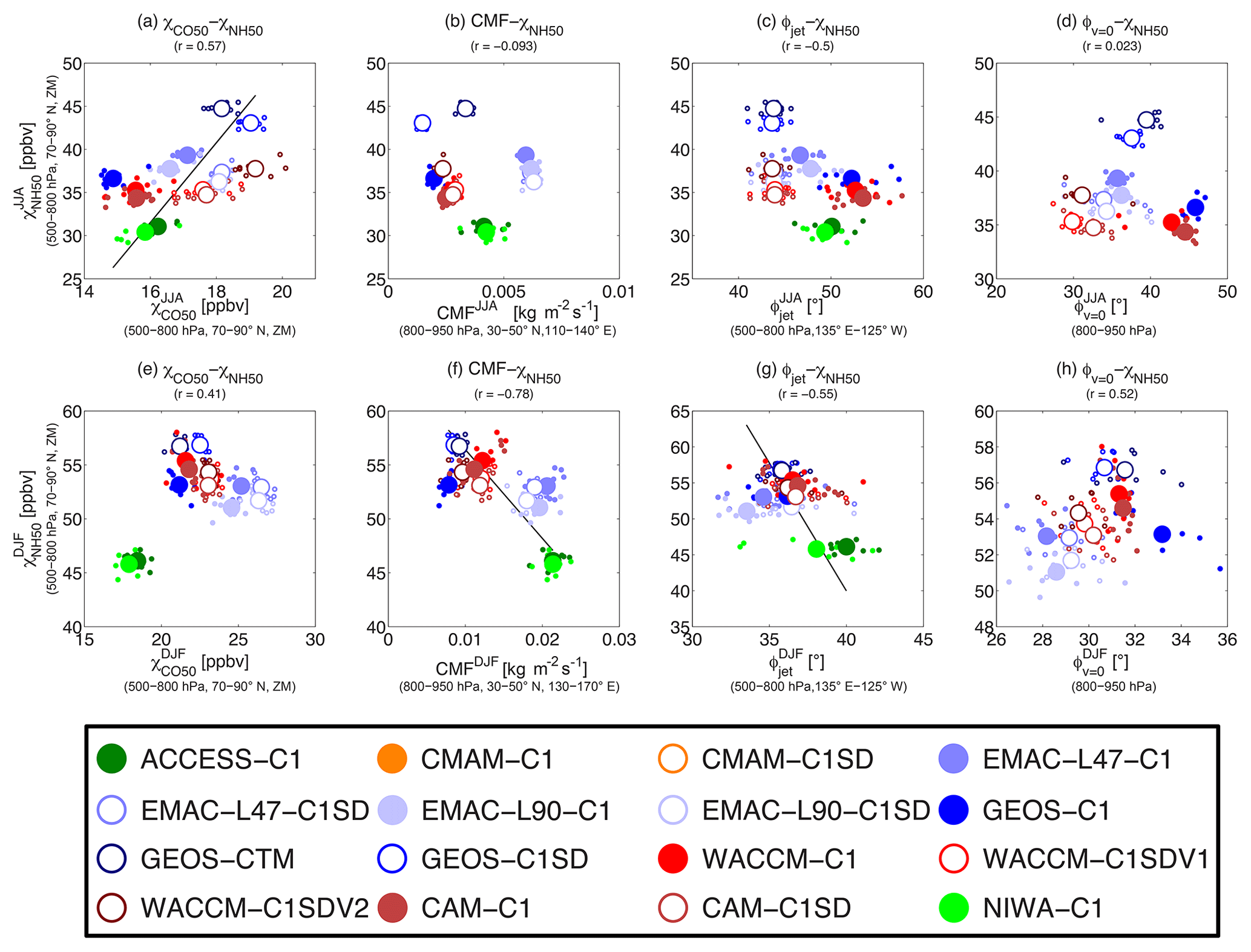
Figure 12(a, e) Tracer–tracer correlation between NH50 and CO50 over the Arctic (500–800 hPa, 70–90∘ N, ZM), (b, f) as in Fig. 3, (c, g) as in Fig. 6, and (d, h) as in Fig. 10b, e, except the y axis is replaced as the Arctic NH50 concentration. Results for JJA are shown in (a)–(d), while those for DJF are shown in (e)–(h).
To explore the relative role of changes in CMF, latitude of the Pacific jet (ϕjet), and HC extent (ϕv=0) in causing the spread in the Arctic NH50, we repeat the above analyses in Sect. 4, and examine the correlations of Arctic concentrations of NH50 with different quantities; see Fig. 12. In contrast to CO50, there is a stronger relationship of NH50 with CMF during winter (see Fig. 12f) but still a weak correlation during summer. Consistent with the study of Orbe et al. (2018) for NH5, Arctic NH50 concentrations tend to be lower in simulations that feature larger low-level midlatitude CMF and such a correlation is weaker in summer. The summertime CMF–NH50 correlation (−0.09) is much lower than the CMF–NH5 correlation (−0.45) reported by Orbe et al. (2018). This is not due to a difference between NH50 and NH5 but rather different models used in the two studies. GEOS-CTM is included here but not by Orbe et al. (2018), and it has higher NH50 than models with similar CMF (and lowers the correlation). At the same time Meteorological Research Institute (MRI) simulations are included by Orbe et al. (2018), but not here (as they do not include the CO50 tracer). These MRI results have high CMF and low NH5 and thus increase the correlation.
Unlike CO50, NH50 exhibits only a moderate or weak correlation with ϕjet and ϕv=0. Note that the ϕjet–NH50 seems to be stronger during winter (−0.5), but this correlation is largely due to the ACCESS and NIWA results. Without these two models, a moderate positive correlation is found instead, which is consistent with Fig. 12g showing a moderate ϕv=0–NH50 correlation during winter.
In summary, despite NH50 having a zonally uniform boundary condition, the multi-model spread of Arctic NH50 seems to be much less impacted by differences in the HC extent and associated zonal-mean transport among the models. Instead, NH50 shows a stronger correlation with low-level midlatitude convection, especially during boreal winter, as shown by Orbe et al. (2018). Therefore, in contrast to a minor role for transporting CO50 towards the Arctic, midlatitude convection predominantly contributes to the inter-model variations in Arctic NH50 concentrations in winter. In summer, convection may play a role as important as the HC extent (as for CO50), but the two processes may act oppositely so that correlations of summertime NH50 are weaker for both. The above results again suggest that transport of zonally uniform (or oceanic) tracers differs in pathways compared to land tracers, and low-level convection over the oceans seems to play a more significant role. Another possible contributor to the CO50–NH50 differences could be the different latitudes of their sources, with NH50 further north than CO50. This possibility needs further analysis.
5.2 CO
It is also of interest to examine whether the above conclusions based on idealized tracers apply to more realistic tracers with interactive chemistry. We therefore examine whether the spread, and relationship with the HC extent (i.e., ϕv=0), found in CO50 can also be found in full chemistry simulations of CO from the CCMI models.
The comparison of CO50 and CO from CCMI results shows a positive relationship between the Arctic concentration of CO50 and CO in winter, but no relationship in summer; see Fig. 13a and c. This suggests that differences in transport that cause differences in CO50 might explain a significant fraction of the multi-model spread of CO during winter when chemistry is relatively weak, but these transport differences are likely less important during summer when model differences in chemistry dominate. This is borne out in Fig. 13b and d, which shows a weak–moderate negative relationship between ϕv=0 and χCO50 during winter but no relationship during summer. This indicates that chemistry may still determine the spatial distribution of real tracers, especially during summer when tracers are more chemically reactive. As to variations of chemistry among the models, a detailed examination on the spatiotemporal variability of tropospheric OH is needed.

Figure 13Similar to Fig. 12a, c, e, g, but for correlations: (a, c) between χCO and χCO50 and (b, d) between ϕv=0 and χCO; during DJF in (a) and (b) and JJA in (c) and (d).
In addition to chemistry, differences in emissions between CO and CO50 are also likely to result in their different sensitivities to variations in the HC extent among the models. In particular, CO features an additional summertime emission source from biomass burning over Siberia, which is in close proximity to the Arctic and hence tends to have a strong influence on the Arctic CO concentration. However, this emission region is distant from the HC edge over the NH midlatitudes, and tracer transport from this higher-latitude region is less likely to be impacted by variations in the HC extent.
In this study, we examine long-range transport into the Arctic using an idealized CO5O tracer with predominantly midlatitude Asian emissions in simulations from a suite of CCMs. There is a wide spread (25 %–45 %) of the Arctic concentrations of CO50 among the simulations, indicating a large inter-model variability in the simulated NH midlatitude-to-Arctic transport. Further, this spread is found to be correlated with the variation in the location of the Pacific jet among the models, with lower Arctic tracer concentrations for a more northern Pacific jet. While the inter-model spread in transport to the Arctic is associated with the latitude of the jet, our analysis indicates that this may be an indirect relationship, with difference in the mean meridional flow (that is correlated with the jet latitude) being the cause of differences in the poleward transport of tracers. Specifically, in models with a more northern jet, the Hadley Cell (HC) generally extends further north and the tracer's source region is mostly covered by the lower branch of the HC with southward surface flow, resulting in less poleward transport. Differences in midlatitude convection among the models appear to play a secondary role.
While the inter-model spread in Arctic CO50 concentrations is largely determined by the HC-related mean meridional transport, this is not the case for the NH50 tracer that features zonally uniform midlatitude sources, which shows a larger correlation with midlatitude convection over the Pacific Ocean during winter, as shown for NH5 by Orbe et al. (2018). Thus, it is likely that variations in convection over the oceans are more efficient in influencing the transport of trace species towards the Arctic than variations in surface meridional flow during winter. Specifically, for NH50 that has similar sources from oceans and lands, the role of convection over the oceans overweights the influence of surface meridional flow. In contrast, for CO50, which has emissions primarily over land, variations in convection over the oceans are remote and less influential and therefore zonal-mean transport by surface meridional flow dominates. In summer, the relative importance of convection versus HC extent is more complex for NH50, suggesting comparable and offsetting effects from both convection and surface meridional flow.
The free-running model C1 simulations have a jet on average further poleward than observed during summer (a common bias in climate models; Barnes and Simpson, 2017), with a corresponding bias in the latitudinal extent of the HC. The correlation between the transport into the Arctic and the latitude of the jet (or the HC edge) then implies that these models likely underestimate the transport into the Arctic. While we have focused on impacts on the CO50 and NH50 tracers, this bias likely exists for the transport of other tracers with predominantly land sources and relatively long lifetimes. Therefore, free-running climate models may underestimate the rate of transport into the Arctic for radiatively important land-based gases, especially during summer.
The specified dynamics simulations (C1SD), which use the same (or very similar) specified meteorological fields, do not have bias in jet location, but, surprisingly, there is a spread in the latitude where v=0 (i.e., ϕv=0), which results in a spread in the rate of transport into the Arctic. Orbe et al. (2017b, 2018) also noted a spread in the transport among C1SD simulations, which they related to the spread in transport due to differences in the parameterized convective mass fluxes. Here we suggest that variations in near-surface v are also a major contributor to differences in transport among C1SD models. Analysis of other metrics of the HC extent show agreement among C1SD simulations for a metric based on u (latitude where surface zonal wind vanishes) but a larger spread for a metric based on v (latitude where mean meridional stream function at 500 hPa switches the sign) (Clara Orbe, personal communication, 2018). It is an open question as to why the C1SD simulations agree on the latitude of the Pacific jet but not on the latitude where v=0, or more fundamentally, why u is constrained while v is not. This needs more analysis in future studies.
The results presented here suggest that differences in the HC extent and associated mean meridional transport are a major factor in causing the large spread in Arctic CO50 among the models. However, the rather small number of models available and the wide range of differences among these models limits how strong conclusions can be made about the relative importance of different processes. To be more definitive, studies are required where individual aspects of a model (or models) are varied to isolate the role of this process in the transport into the Arctic. Such experiments are planned for the future.
Most of data from CCMI-1 used in this study can be obtained through the British Atmosphere Data Centre (BADC) archive (ftp://ftp.ceda.ac.uk, last access: 6 July 2018). Data from the Community Earth System Model (CESM) can be obtained through the Climate Data Gateway at the National Center for Atmospheric Research (NCAR) (https://www.earthsystemgrid.org/search.html?Project=CCMI1, last access: 6 July 2018). For instructions for access to both archives, see http://blogs.reading.ac.uk/ccmi/badc-data-access/ (last access: 2 August 2018).
The supplement related to this article is available online at: https://doi.org/10.5194/acp-19-5511-2019-supplement.
HY performed the analysis and wrote the paper; DWW supervised the project and participated in paper editing. CO helped in collecting model output, and performed GEOS simulations with daily output as well as paper editing. GZ, OM, DEK, JFL, ST, DAP, PJ, SES, KAS, and RS all helped in providing model outputs and suggestions for paper editing.
The authors declare that they have no conflict of interest.
This article is part of the special issue “Chemistry-Climate Modelling Initiative (CCMI) (ACP/AMT/ESSD/GMD inter-journal SI)”. It is not associated with a conference.
We thank the Centre for Environmental Data Analysis (CEDA) for hosting the CCMI data archive. We acknowledge the modeling groups for making their simulations available for this analysis and the joint WCRP SPARC/IGAC Chemistry–Climate Model Initiative (CCMI) for organizing and coordinating this model data analysis activity. In addition, Clara Orbe would like to acknowledge the high-performance computing resources provided by the NASA Center for Climate Simulation (NCCS) and support from the NASA Modeling, Analysis and Prediction (MAP) program. Olaf Morgenstern and Guang Zeng acknowledge the UK Met Office for use of the MetUM. Their research was supported by the New Zealand government's Strategic Science Investment Fund (SSIF) through the NIWA program CACV. Olaf Morgenstern acknowledges funding by the New Zealand Royal Society Marsden Fund (grant 12-NIW-006) and by the Deep South National Science Challenge (http://www.deepsouthchallenge.co.nz, last access: 13 April 2019). Olaf Morgenstern and Guang Zeng also wish to acknowledge the contribution of the NeSI high-performance computing facilities to the results of this research. New Zealand's national facilities are provided by the New Zealand eScience Infrastructure (NeSI) and funded jointly by NeS's collaborator institutions and through the Ministry of Business, Innovation and Employment's Research Infrastructure program (https://www.nesi.org.nz, last access: 13 April 2019). Huang Yang and Darryn W. Waugh acknowledge support from NSF grant AGS-1403676. Darryn W. Waugh acknowledges NASA grant NNX14AP58G. Huang Yang thanks discussions with Luke D. Oman and the co-editor Peter Hess. The EMAC model simulations have been performed at the German Climate Computing Centre (DKRZ) through support from the Bundesministerium für Bildung und Forschung (BMBF). DKRZ and its scientific steering committee are gratefully acknowledged for providing the HPC and data archiving resources for the consortial project ESCiMo (Earth System Chemistry integrated Modeling). Robyn Schofield and Kane A. Stone acknowledge support from the Australian Research Council's Centre of Excellence for Climate System Science (CE110001028), the Australian government's National Computational Merit Allocation Scheme (q90), and the Australian Antarctic science grant program (FoRCES 4012).
This paper was edited by Peter Hess and reviewed by three anonymous referees.
Bacmeister, J. T., Suarez, M. J., and Robertson, F. R.: Rain Reevaporation, Boundary Layer–Convection Interactions, and Pacific Rainfall Patterns in an AGCM, J. Atmos. Sci., 63, 3383–3403, https://doi.org/10.1175/JAS3791.1, 2006. a, b, c
Barnes, E. A. and Polvani, L.: Response of the midlatitude jets, and of their variability, to increased greenhouse gases in the CMIP5 models, J. Climate, 26, 7117–7135, https://doi.org/10.1175/JCLI-D-12-00536.1, 2013. a, b
Barnes, E. A. and Simpson, I. R.: Seasonal sensitivity of the Northern Hemisphere jet streams to Arctic temperatures on subseasonal time scales, J. Climate, 30, 10117–10137, https://doi.org/10.1175/JCLI-D-17-0299.1, 2017. a, b
Bottenheim, J. W., Dastoor, A., Gong, S. L., Higuchi, K., and Li, Y. F.: Long Range Transport of Air Pollution to the Arctic, in: Handbook of Environmental Chemistry, vol. 4G, 13–39, Springer, Berlin, Heidelberg, https://doi.org/10.1007/b94522, 2004. a
Bowman, K. P. and Carrie, G. D.: The Mean-Meridional Transport Circulation of the Troposphere in an Idealized GCM, J. Atmos. Sci., 59, 1502–1514, 2002. a
Coopman, Q., Garrett, T. J., Finch, D. P., and Riedi, J.: High Sensitivity of Arctic Liquid Clouds to Long-Range Anthropogenic Aerosol Transport, Geophys. Res. Lett., 45, 372–381, https://doi.org/10.1002/2017GL075795, 2018. a
Doherty, R. M., Orbe, C., Zeng, G., Plummer, D. A., Prather, M. J., Wild, O., Lin, M., Shindell, D. T., and Mackenzie, I. A.: Multi-model impacts of climate change on pollution transport from global emission source regions, Atmos. Chem. Phys., 17, 14219–14237, https://doi.org/10.5194/acp-17-14219-2017, 2017. a
Eckhardt, S., Stohl, A., Beirle, S., Spichtinger, N., James, P., Forster, C., Junker, C., Wagner, T., Platt, U., and Jennings, S. G.: The North Atlantic Oscillation controls air pollution transport to the Arctic, Atmos. Chem. Phys., 3, 1769–1778, https://doi.org/10.5194/acp-3-1769-2003, 2003. a
Eyring, V., Lamarque, J.-F., Hess, P., Arfeuille, F., Bowman, K., Chipperfield, M. P., Duncan, B., Fiore, A., Gettelman, A., Giorgetta, M. A., Granier, C., Hegglin, M., Kinnison, D., Kunze, M., Langematz, U., Luo, B., Martin, R., Matthes, K., Newman, P. A., Peter, T., Robock, A., Ryerson, T., Saiz-Lopez, A., Salawitch, R., Schultz, M., Shepherd, T. G., Shindell, D., Stähelin, J., Tegtmeier, S., Thomason, L., Tilmes, S., Vernier, J.-P., Waugh, D. W., and Young, P. J.: Overview of IGAC/SPARC Chemistry-Climate Model Initiative (CCMI) Community Simulations in Support of Upcoming Ozone and Climate Assessments, SPARC Newsletter, 40, 48–66, 2013. a, b
Fang, Y., Fiore, A. M., Horowitz, L. W., Gnanadesikan, A., Held, I., Chen, G., Vecchi, G., and Levy, H.: The impacts of changing transport and precipitation on pollutant distributions in a future climate, J. Geophys. Res.-Atmos., 116, 1–14, https://doi.org/10.1029/2011JD015642, 2011. a
Fisher, J. A., Jacob, D. J., Purdy, M. T., Kopacz, M., Le Sager, P., Carouge, C., Holmes, C. D., Yantosca, R. M., Batchelor, R. L., Strong, K., Diskin, G. S., Fuelberg, H. E., Holloway, J. S., Hyer, E. J., McMillan, W. W., Warner, J., Streets, D. G., Zhang, Q., Wang, Y., and Wu, S.: Source attribution and interannual variability of Arctic pollution in spring constrained by aircraft (ARCTAS, ARCPAC) and satellite (AIRS) observations of carbon monoxide, Atmos. Chem. Phys., 10, 977–996, https://doi.org/10.5194/acp-10-977-2010, 2010. a
Garny, H. and Randel, W. J.: Dynamic variability of the Asian monsoon anticyclone observed in potential vorticity and correlations with tracer distributions, J. Geophys. Res. Atmos., 118, 13421–13433, https://doi.org/10.1002/2013JD020908, 2013. a
Garrett, T. J. and Zhao, C.: Increased Arctic cloud longwave emissivity associated with pollution from mid-latitudes, Nature, 440, 787–789, https://doi.org/10.1038/nature04636, 2006. a
Hack, J. J.: Parameterization of moist convection in the National Center for Atmospheric Research community climate model (CCM2), J. Geophys. Res., 99, 5551–5568, https://doi.org/10.1029/93JD03478, 1994. a, b, c, d, e
Haynes, P. and Shuckburgh, E.: Effective diffusivity as a diagnostic of atmospheric transport 2. Troposphere and lower stratosphere, J. Geophys. Res., 105, 22795–22810, 2000. a
Hewitt, H. T., Copsey, D., Culverwell, I. D., Harris, C. M., Hill, R. S. R., Keen, A. B., McLaren, A. J., and Hunke, E. C.: Design and implementation of the infrastructure of HadGEM3: the next-generation Met Office climate modelling system, Geosci. Model Dev., 4, 223–253, https://doi.org/10.5194/gmd-4-223-2011, 2011. a, b
Holloway, T., Levy II, H., and Kasibhatla, P.: Global distribution of carbon monoxide, J. Geophys. Res., 105, 12123–12147, 2000. a
IPCC: Climate Change 2013: The Physical Science Basis, Contribution of Working Group I to the Fifth Assessment Report of the Intergovernmental Panel on Climate Change, Cambridge University Press, Cambridge, United Kingdom and New York, NY, USA, https://doi.org/10.1029/2000JD000115, 2013. a
Kupiszewski, P., Leck, C., Tjernström, M., Sjogren, S., Sedlar, J., Graus, M., Müller, M., Brooks, B., Swietlicki, E., Norris, S., and Hansel, A.: Vertical profiling of aerosol particles and trace gases over the central Arctic Ocean during summer, Atmos. Chem. Phys., 13, 12405–12431, https://doi.org/10.5194/acp-13-12405-2013, 2013. a
Lubin, D. and Vogelmann, A. M.: A climatologically significant aerosol longwave indirect effect in the Arctic, Nature, 439, 453–456, https://doi.org/10.1038/nature04449, 2006. a
Moorthi, S. and Suarez, M. J.: Relaxed Arakawa-Schubert, A Parameterization of Moist Convection for General Circulation Models, Mon. Weather Rev., 120, 978–1002, https://doi.org/10.1175/1520-0493(1992)120<0978:RASAPO>2.0.CO;2, 1992. a, b, c
Morgenstern, O., Hegglin, M. I., Rozanov, E., O'Connor, F. M., Abraham, N. L., Akiyoshi, H., Archibald, A. T., Bekki, S., Butchart, N., Chipperfield, M. P., Deushi, M., Dhomse, S. S., Garcia, R. R., Hardiman, S. C., Horowitz, L. W., Jöckel, P., Josse, B., Kinnison, D., Lin, M., Mancini, E., Manyin, M. E., Marchand, M., Marécal, V., Michou, M., Oman, L. D., Pitari, G., Plummer, D. A., Revell, L. E., Saint-Martin, D., Schofield, R., Stenke, A., Stone, K., Sudo, K., Tanaka, T. Y., Tilmes, S., Yamashita, Y., Yoshida, K., and Zeng, G.: Review of the global models used within phase 1 of the Chemistry–Climate Model Initiative (CCMI), Geosci. Model Dev., 10, 639–671, https://doi.org/10.5194/gmd-10-639-2017, 2017. a, b
Nordeng, T. E.: Extended versions of the convective parametrization scheme at ECMWF and their impact on the mean and transient activity of the model in the tropics, Tech. rep., ECMWF, Reading, UK, 1994. a, b, c
Orbe, C., Oman, L. D., Strahan, S. E., Waugh, D. W., Pawson, S., Takacs, L. L., and Molod, A. M.: Large-Scale Atmospheric Transport in GEOS Replay Simulations, J. Adv. Model. Earth. Sy., 9, 2545–2560, https://doi.org/10.1002/2017MS001053, 2017a. a
Orbe, C., Waugh, D. W., Yang, H., Lamarque, J. F., Tilmes, S., and Kinnison, D. E.: Tropospheric transport differences between models using the same large-scale meteorological fields, Geophys. Res. Lett., 44, 1068–1078, https://doi.org/10.1002/2016GL071339, 2017b. a, b, c, d
Orbe, C., Yang, H., Waugh, D. W., Zeng, G., Morgenstern , O., Kinnison, D. E., Lamarque, J.-F., Tilmes, S., Plummer, D. A., Scinocca, J. F., Josse, B., Marecal, V., Jöckel, P., Oman, L. D., Strahan, S. E., Deushi, M., Tanaka, T. Y., Yoshida, K., Akiyoshi, H., Yamashita, Y., Stenke, A., Revell, L., Sukhodolov, T., Rozanov, E., Pitari, G., Visioni, D., Stone, K. A., Schofield, R., and Banerjee, A.: Large-scale tropospheric transport in the Chemistry–Climate Model Initiative (CCMI) simulations, Atmos. Chem. Phys., 18, 7217–7235, https://doi.org/10.5194/acp-18-7217-2018, 2018. a, b, c, d, e, f, g, h, i, j, k, l, m, n, o, p, q, r, s, t, u, v
Palmer, P. I., Jacob, D. J., Jones, D. B. A., Heald, C. L., Yantosca, R. M., Logan, J. A., Sachse, G. W., and Streets, D. G.: Inverting for emissions of carbon monoxide from Asia using aircraft observations over the western Pacific, J. Geophys. Res.-Atmos., 108, 8828, https://doi.org/10.1029/2003JD003397, 2003. a
Park, M., Randel, W. J., Gettelman, A., Massie, S. T., and Jiang, J. H.: Transport above the Asian summer monsoon anticyclone inferred from Aura Microwave Limb Sounder tracers, J. Geophys. Res.-Atmos., 112, 1–13, https://doi.org/10.1029/2006JD008294, 2007. a
Petráš, I. and Bednárová, D.: Total Least Squares Approach to Modeling: A Matlab Toolbox, Acta Montan. Slovaca, 15, 158–170, 2010. a
Rayner, N. A.: Global analyses of sea surface temperature, sea ice, and night marine air temperature since the late nineteenth century, J. Geophys. Res., 108, 4407, https://doi.org/10.1029/2002JD002670, 2003. a
Shindell, D.: Local and remote contributions to Arctic warming, Geophys. Res. Lett., 34, 1–5, https://doi.org/10.1029/2007GL030221, 2007. a
Shindell, D. T., Chin, M., Dentener, F., Doherty, R. M., Faluvegi, G., Fiore, A. M., Hess, P., Koch, D. M., MacKenzie, I. A., Sanderson, M. G., Schultz, M. G., Schulz, M., Stevenson, D. S., Teich, H., Textor, C., Wild, O., Bergmann, D. J., Bey, I., Bian, H., Cuvelier, C., Duncan, B. N., Folberth, G., Horowitz, L. W., Jonson, J., Kaminski, J. W., Marmer, E., Park, R., Pringle, K. J., Schroeder, S., Szopa, S., Takemura, T., Zeng, G., Keating, T. J., and Zuber, A.: A multi-model assessment of pollution transport to the Arctic, Atmos. Chem. Phys., 8, 5353–5372, https://doi.org/10.5194/acp-8-5353-2008, 2008. a, b, c, d
Staten, P. W. and Reichler, T.: On the ratio between shifts in the eddy-driven jet and the Hadley cell edge, Clim. Dynam., 42, 1229–1242, https://doi.org/10.1007/s00382-013-1905-7, 2014. a
Tiedtke, M.: A Comprehensive Mass Flux Scheme for Cumulus Parameterization in Large-Scale Models, Mon. Weather Rev., 117, 1779–1800, https://doi.org/10.1175/1520-0493, 1989. a, b, c
Wu, X., Yang, H., Waugh, D. W., Orbe, C., Tilmes, S., and Lamarque, J.-F.: Spatial and temporal variability of interhemispheric transport times, Atmos. Chem. Phys., 18, 7439–7452, https://doi.org/10.5194/acp-18-7439-2018, 2018. a
Yu, P., Rosenlof, K. H., Liu, S., Telg, H., Thornberry, T. D., Rollins, A. W., Portmann, R. W., Bai, Z., Ray, E. A., Duan, Y., Pan, L. L., Toon, O. B., Bian, J., and Gao, R.-S.: Efficient transport of tropospheric aerosol into the stratosphere via the Asian summer monsoon anticyclone, P. Natl. Acad. Sci. USA, 114, 6972–6977, https://doi.org/10.1073/pnas.1701170114, 2017. a
Zhang, G. J. and McFarlane, N. A.: Sensitivity of Climate Simulations tothe Parameterization of Cumulus Convection in the Canadian Climate Centre Circulation Model, Atmos. Ocean, 33, 407–446, 1995. a, b, c, d, e, f, g