the Creative Commons Attribution 4.0 License.
the Creative Commons Attribution 4.0 License.
 | 05 Apr 2019
Effects of urbanization on regional meteorology and air quality in Southern California
Yun Li
Jiachen Zhang
David J. Sailor
Urbanization has a profound influence on regional meteorology and air quality in megapolitan Southern California. The influence of urbanization on meteorology is driven by changes in land surface physical properties and land surface processes. These changes in meteorology in turn influence air quality by changing temperature-dependent chemical reactions and emissions, gas–particle phase partitioning, and ventilation of pollutants. In this study we characterize the influence of land surface changes via historical urbanization from before human settlement to the present day on meteorology and air quality in Southern California using the Weather Research and Forecasting Model coupled to chemistry and the single-layer urban canopy model (WRF–UCM–Chem). We assume identical anthropogenic emissions for the simulations carried out and thus focus on the effect of changes in land surface physical properties and land surface processes on air quality. Historical urbanization has led to daytime air temperature decreases of up to 1.4 K and evening temperature increases of up to 1.7 K. Ventilation of air in the LA basin has decreased up to 36.6 % during daytime and increased up to 27.0 % during nighttime. These changes in meteorology are mainly attributable to higher evaporative fluxes and thermal inertia of soil from irrigation and increased surface roughness and thermal inertia from buildings. Changes in ventilation drive changes in hourly NOx concentrations with increases of up to 2.7 ppb during daytime and decreases of up to 4.7 ppb at night. Hourly O3 concentrations decrease by up to 0.94 ppb in the morning and increase by up to 5.6 ppb at other times of day. Changes in O3 concentrations are driven by the competing effects of changes in ventilation and precursor NOx concentrations. PM2.5 concentrations show slight increases during the day and decreases of up to 2.5 µg m−3 at night. Process drivers for changes in PM2.5 include modifications to atmospheric ventilation and temperature, which impact gas–particle phase partitioning for semi-volatile compounds and chemical reactions. Understanding process drivers related to how land surface changes effect regional meteorology and air quality is crucial for decision-making on urban planning in megapolitan Southern California to achieve regional climate adaptation and air quality improvements.
- Article
(4600 KB) - Full-text XML
-
Supplement
(2306 KB) - BibTeX
- EndNote


The world has been undergoing accelerated urbanization since the industrial revolution in the 19th century (Grimm et al., 2008; Seto et al., 2012). Urbanization leads to profound human modification of the land surface and its associated physical properties such as roughness, thermal inertia, and albedo (Fan et al., 2017) and land surface processes like irrigation (Vahmani and Hogue, 2014). These changes in land surface physical properties and processes alter corresponding surface–atmosphere coupling including exchange of water, momentum, and energy in urbanized regions (Vahmani and Ban-Weiss, 2016a; Li et al., 2017), which exerts an important influence on regional meteorology and air quality (Vahmani et al., 2016; Civerolo et al., 2007).
Land surface modifications from urbanization drive changes in urban meteorological variables such as temperature, wind speed, and planetary boundary layer (PBL) height, which result in urban–rural differences. Differences in surface temperature and near-surface air temperature have been widely studied for decades. The urban heat island (UHI) effect, a phenomenon in which temperatures within an urban area are higher than surrounding rural areas (Oke, 1982), has been extensively studied using models and observations for a great number of urban regions (Rizwan et al., 2008; Peng et al., 2012; Stewart and Oke, 2012). A contrary phenomenon, namely the urban cool island (UCI), under which urban temperatures are lower than surrounding rural temperatures, has also been investigated recently in some studies (Carnahan and Larson, 1990; Theeuwes et al., 2015; Kumar et al., 2017). Urban–rural contrast in temperature (i.e., both UHI and UCI) is mainly attributable to differences in thermal properties and energy fluxes due to heterogeneous land surface properties. For urban areas, buildings and roads (i.e., impervious surfaces) are generally made from manufactured materials (e.g., asphalt concrete) with low albedo and thus high solar absorptivity (Wang et al., 2017). These materials also have high thermal inertia, which can lead to reductions in diurnal temperature range due to heat storage and consequent temperature reductions during the day and heat release and consequent temperature increases at night (Hardin and Vanos, 2018). Street canyons, which we refer to as the U-shaped region between buildings, can trap longwave energy fluxes within the canyon because of reductions of sky-view factors (Qiao et al., 2013). Conversely, shading in street canyons during the day can reduce absorption of shortwave radiation (Carnahan and Larson, 1990; Kusaka et al., 2001). Pervious surfaces within urban areas such as irrigated urban parks and lawns can lead to the urban oasis effect in which evaporative cooling occurs due to increases in evapotranspiration. In addition, soil thermal properties depend on their water content, which ultimately affects ground heat fluxes and thus surface and air temperatures. Land surface properties in surrounding rural areas can also affect urban–rural differences in temperature (Imhoff et al., 2010; Peng et al., 2012; Zhao et al., 2014). In particular, urban regions built in semiarid or arid surroundings tend to have a weak daytime UHI or even a UCI, whereas those built in moist regions tend to have a larger daytime UHI (Fan et al., 2017; Peng et al., 2012). Lastly, factors such as anthropogenic heat and atmospheric aerosol burdens can play an important role in urban heat or cool island formation in some regions (Oke, 1982; Wang et al., 2017).
Urbanization can also cause differences between urban and rural areas for meteorological variables other than surface and air temperatures. Changes in regional near-surface wind speed and direction can occur in urban areas because of spatially varying modifications in surface roughness (Xu et al., 2006; Vahmani et al., 2016). Changes in near-surface winds in coastal urban areas can also be affected by modifying land–sea temperature contrast (Vahmani et al., 2016). The characteristics of the PBL are dependent on the magnitude of turbulent kinetic energy (TKE) (Garratt, 1994). Higher (lower) TKE will lead to deeper (shallower) PBLs. During daytime, the magnitude of TKE is driven by buoyancy production contributed mainly by sensible heat flux (with clear skies); at night, TKE is driven by shear production associated with variance in wind speed. Thus, temperature and surface roughness play an important role in the depth of the PBL during daytime and nighttime, respectively. Lastly, changes in relative humidity, precipitation, and other meteorological variables due to land surface changes can also be significant in some regions (Burian and Shepherd, 2005; Georgescu et al., 2014).
Changes in meteorological conditions due to urbanization can influence concentrations of air pollutants including oxides of nitrogen (NOx), ozone (O3), and fine particulate matter (PM2.5). NOx and O3 pollution are major public health concerns in megapolitan regions (Lippmann, 1989). PM2.5 reduces visibility, causes adverse health effects, and alters regional and global climate via direct and indirect effects (Charlson et al., 1992; Pope and Dockery, 2006; Boucher et al., 2013). Meteorology can affect emission rates (e.g., biogenic volatile organic compounds (BVOCs) and evaporative emissions of gasoline), chemical reaction rates, gas–particle phase partitioning of semi-volatile species, pollutant dispersion, and deposition; thus, it plays an important role in determining air pollutant concentrations. Variations in air temperatures together with vegetation types affect the production of BVOCs, which are important precursors for ground-level O3 and secondary organic aerosols (SOAs) (Guenther et al., 2006). Gas-phase chemical reactions that form secondary pollutants are also temperature dependent. Higher (lower) air temperatures in general lead to higher (lower) photolysis reaction rates and atmospheric oxidation rates, which enhance the production of tropospheric O3, secondary inorganic aerosols (e.g., nitrate, sulfate, and ammonium aerosols) and SOA (Aw and Kleeman, 2003; Hassan et al., 2013). In addition, concentrations of semi-volatile compounds are affected by equilibrium vapor pressure under various temperature conditions (Pankow, 1997; Ackermann et al., 1998). Higher (lower) temperatures favor phase-partitioning to the gas (particle) phase. Ventilation, which is the combined effect of vertical mixing and horizontal dispersion, can also influence pollutant concentrations (Epstein et al., 2017). Higher (lower) ventilation rates lead to lower (higher) pollutant concentrations, especially in coastal cities like Los Angeles where upwind air under typical meteorological conditions is clean relative to urban air. Lastly, changes in surface roughness may affect loss of pollutants via surface deposition, which in turn alters air pollutant concentrations (Abdul-Wahab et al., 2005).
A number of previous studies have investigated the impacts of land surface changes on regional meteorology in a variety of urban regions around the world (e.g., Kalnay and Cai, 2003; Burian and Shepherd, 2005; Zhang et al., 2010). However, limited studies have quantified the impact of land surface changes on regional air quality, and those that do exist have focused on only changes in surface O3 concentrations. Civerolo et al. (2007) estimated that land-use changes via urban expansion in New York City can cause increases in near-surface air temperature of 0.6 ∘C as well as increases in episode-maximum 8 h O3 concentrations of +6 ppb. Jiang et al. (2008) focused on the Houston, Texas, area and found similar relationships between urban expansion, near-surface air temperatures, and O3. Nevertheless, only a few studies have included changes in PM2.5 concentrations. Tao et al. (2015) simulated that spatially averaged surface O3 concentrations slightly increased (+0.1 ppb) in eastern China due to urbanization, whereas PM2.5 concentrations decreased by −5.4 µg m−3 at the near surface. Chen et al. (2018) studied urbanization in Beijing and found that modification of rural to urban land surfaces has led to increases in near-surface air temperature and PBL height, which in turn led to increases (+9.5 ppb) in surface O3 concentrations and decreases (−16.6 µg m−3) in PM2.5 concentrations. However, past studies that investigate interactions between land surface changes and changes in meteorology and air quality generally do not identify the major processes driving these interactions. They also do not resolve the wide spatial heterogeneity of urban land surface properties, with most studies assuming that urban properties are homogenous throughout the city. In addition, only a few studies investigate interactions between land surface changes and air quality for the Southern California region (Taha, 2015; Epstein et al., 2017; Zhang et al., 2018b), which is one of the most polluted areas in the United States (American Lung Association, 2012).
With advances in real-world land surface datasets from satellites, recent modeling studies on land–atmosphere interactions are able to resolve heterogeneous land surface properties and thus better capture urban meteorology, enabling modeling studies that more accurately quantify changes in regional meteorology due to land surface modification. By combining satellite-retrieved high-resolution land surface data with the Weather Research and Forecasting Model coupled to the single-layer urban canopy model (WRF–UCM), simulations reported in Vahmani and Ban-Weiss (2016a) show improved model performance (i.e., compared to observations) for meteorology in Southern California compared to the default model, which assumes that urban regions have homogeneous urban land cover. In a follow-up study, Vahmani et al. (2016) suggested that historical urbanization has altered regional meteorology (e.g., near-surface air temperatures and wind flows) in Southern California mainly because of urban irrigation and changes in land surface thermal properties and roughness. While historical urbanization and its associated impacts on meteorology have the potential to cause important changes in air pollutant concentrations in Southern California, this has never been investigated in past work.
Therefore, this study aims to characterize the influence of land surface changes via historical urbanization on urban meteorology and air quality in Southern California by comparing a “present-day” scenario with current urban land surface properties and land surface processes to a “nonurban” scenario assuming land surface distributions prior to human perturbation. To achieve this goal, we adopt a state-of-the-science regional climate–air quality model, the Weather Research and Forecasting Model coupled to chemistry and the single-layer urban canopy model (WRF–UCM–Chem), and incorporate high-resolution heterogeneity in urban surface properties and processes to predict regional weather and pollutant concentrations. We assess the response of regional meteorology and air quality to individual changes in land surface properties and processes to determine driving factors on atmospheric changes. Note that this paper builds on our prior study Vahmani et al. (2016) but focuses on air quality impacts, whereas our previous research was on meteorological impacts only. While the influence of land surface changes on regional weather has been investigated in numerous past studies, its influence on regional air quality has been seldom studied in past work. In this paper, we aim to quantify the importance of historical land cover change on air pollutant concentrations, and thus the nonurban scenario assumes current anthropogenic pollutant emissions. This hypothetical scenario cannot exist in reality since current anthropogenic emissions would not exist without the city, but our intent is to tease out the relative importance of land cover change through urbanization (assuming constant emissions) on air pollutant concentrations.
2.1 Model description and configuration
WRF-Chem v3.7 is used in this study to simulate meteorological fields and atmospheric chemistry. WRF-Chem is a state-of-the-science nonhydrostatic mesoscale numerical meteorological model that facilitates “online” simulation of processes relevant to atmospheric chemistry including pollutant emissions, gas- and particle-phase chemistry, transport and mixing, and deposition (Grell et al., 2005). In this study, we activate the urban canopy model (UCM) in WRF-Chem that resolves land–atmosphere exchange of water, momentum, and energy for impervious surfaces in urban areas (Kusaka et al., 2001; Chen et al., 2011; Yang et al., 2015). The UCM parameterizes the effects of urban geometry on energy fluxes from urban facets (i.e., roofs, walls, and roads) and wind profiles within canyons (Kusaka et al., 2012). We account for the effect of anthropogenic heat on urban climate by adopting the default diurnal profile in the UCM. We used UCM instead of the multilayer canopy layer model (BEP) because BEP would increase computational costs, but for likely little additional benefit in the quality of simulations (Chen et al., 2011; Kusaka et al., 2001). Physics schemes included in our model configuration are the Lin cloud microphysics scheme (Lin et al., 1983), the RRTM longwave radiation scheme (Mlawer et al., 1997), the Goddard shortwave radiation scheme (Chou and Suarez, 1999), the YSU boundary layer scheme (Hong et al., 2006), the MM5 similarity surface layer scheme (Dyer and Hicks, 1970; Paulson, 1970), the Grell 3-D ensemble cumulus cloud scheme (Grell and Dévényi, 2002), and the unified Noah land surface model (Chen et al., 2001). Chemistry schemes include the TUV photolysis scheme (Madronich, 1987), RACM-ESRL gas-phase chemistry (Kim et al., 2009; Stockwell et al., 1997), and MADE/VBS aerosol scheme (Ackermann et al., 1998; Ahmadov et al., 2012).
All model simulations are carried out from 28 June, 21:00 UTC (28 June, 13:00 PST) to 8 July, 07:00 UTC (7 July, 23:00 PST), 2012 using the North American Regional Reanalysis (NARR) dataset as initial and boundary meteorological conditions (Mesinger et al., 2006). This simulation period is chosen as representative of typical summer days in Southern California, which are generally clear or mostly sunny without precipitation. A comparison of observed diurnal cycles for average near-surface air temperatures over JJA (June, July, and August) in the year 2012 versus over our simulation period is shown in Fig. S8 in the Supplement. Hourly model output from 1 July, 00:00 PST to 7 July, 23:00 PST is used for analysis, and simulation results prior to 1 July, 00:00 PST are discarded as spin-up. Figure 1a shows the three two-way nested domains with horizontal resolutions of 18, 6, and 2 km centered at 33.9∘ N, 118.14∘ W. Only the innermost domain (141×129 grid cells), which encapsulates the Los Angeles and San Diego metropolitan regions, is used for analysis. All three domains consist of 29 unequally spaced layers in the vertical from the ground to 100 hPa. The average depth of the lowest model level is 53 m for all three domains.
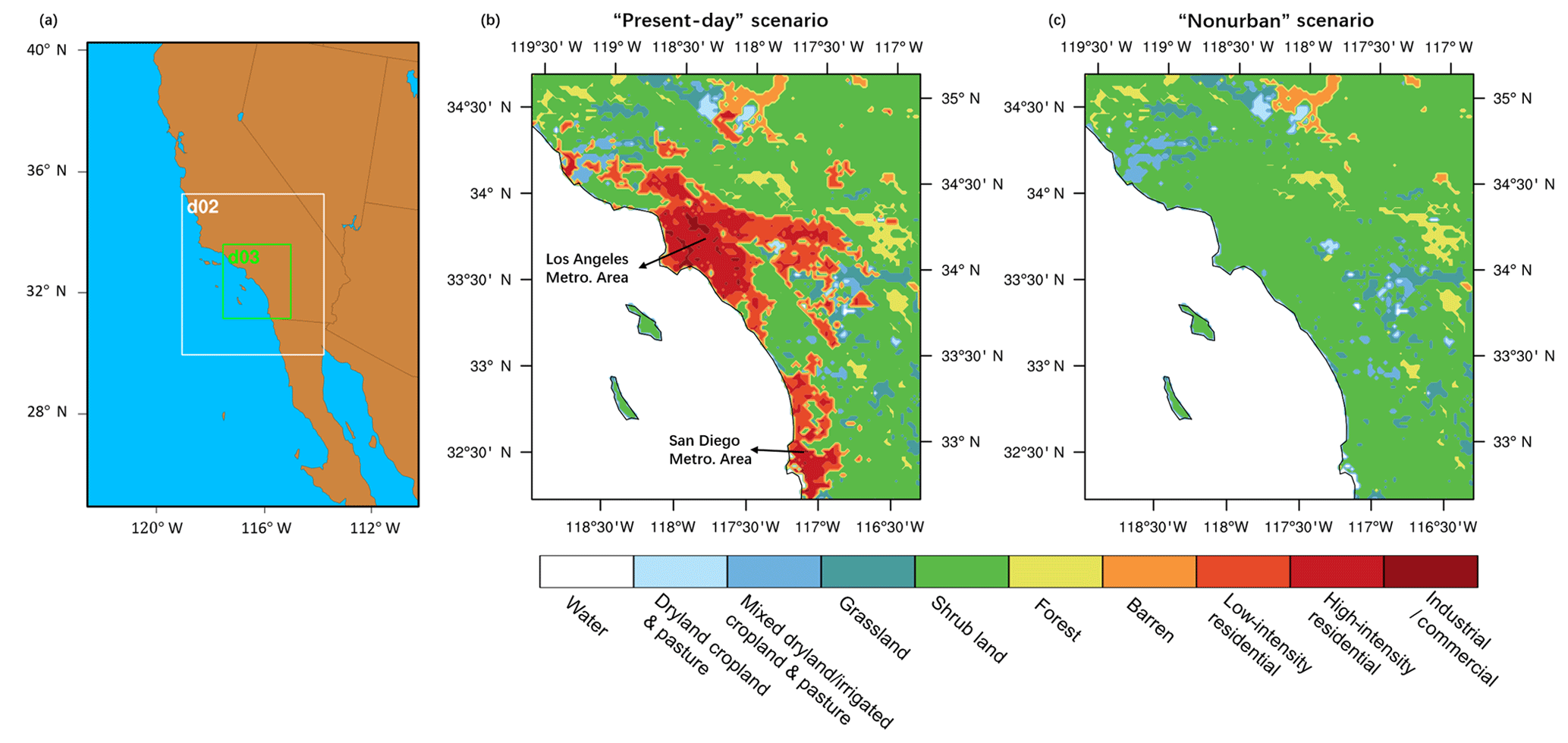
Figure 1Maps of (a) the three nested WRF–UCM–Chem domains and (b, c) land cover types for the innermost domain (d03) for the (b) present-day and (c) nonurban scenarios.
2.2 Land surface property characterization and irrigation parameterization
One important aspect of accurately simulating meteorology and air quality is to properly characterize land surface–atmosphere interactions (Vahmani and Ban-Weiss, 2016a; Li et al., 2017). In addition, accurately quantifying the climate and air quality impacts of historical urbanization requires a realistic portrayal of current land cover in the urban area (Vahmani et al., 2016). For both of these reasons, we update the default WRF-Chem to include a real-world representation of land surface physical properties and processes.
In this study, we use the (30 m resolution) 33-category National Land Cover Database (NLCD) for the year 2006 for all three model domains. NLCD differentiates three urban types including low-intensity residential, high-intensity residential, and industrial/commercial (shown in Fig. 1b) (Fry et al., 2011). In the model (UCM), each of these three types can have unique urban physical properties such as building morphology, albedo, and thermal properties for each facet. We adopt the grid-cell-specific National Urban Database and Access Portal Tool (NUDAPT) where available in the innermost domain for building morphology including average building heights, road widths, and roof widths (Ching et al., 2009). Where NUDAPT data are unavailable, we use average building and road morphology for three urban categories from the Los Angeles Region Imagery Acquisition Consortium (LARIAC). Details on the generation of averaged urban morphology parameters from real-world GIS datasets can be found in Zhang et al. (2018a). For the other parameters in the UCM (e.g., anthropogenic latent heat, surface emissivity), we use default WRF settings documented in file URBPARM.TBL. Note that the original gaseous dry deposition code based on Wesely (1989) is only compatible with the default 24-category US Geological Survey (USGS) global land cover map. We therefore modify the code according to Fallmann et al. (2016), which assumes that the three urban types in the 33-category system have input resistances that are the same as the urban type for the 24-category system. In addition, impervious fractions (i.e., the fraction of each cell covered by impervious surfaces) for each of the three urban categories in the innermost domain are from the NLCD impervious surface data (Wickham et al., 2013).
Land surface properties including albedo, green vegetation fraction (GVF), and leaf area index (LAI) are important for accurately predicting absorption and reflection of solar radiation and evaporative fluxes in urban areas (Vahmani and Ban-Weiss, 2016a). To resolve high-resolution real-world heterogeneity in these land surface properties, the simulations performed in this study use satellite-retrieved real-time albedo, GVF, and LAI for the innermost domain. Input data compatible with WRF are regridded horizontally using albedo, GVF, and LAI maps generated based on MODIS reflectance (MCD43A4), vegetation indices (MOD13A3), and fraction of photosynthetically active radiation (MCD15A3) products, respectively. Raw data are available from the USGS National Center for Earth Resource Observations and Science website at http://earthexplorer.usgs.gov (last access: 27 May 2015). A detailed description on the implementation of MODIS-retrieved land surface properties for WRF can be found in Vahmani and Ban-Weiss (2016a). Our previous research has shown that the model enhancements described here reduce model biases in surface and near-surface air temperatures (relative to ground and satellite observations) for urban regions in Southern California. In particular, the root-mean-square-error for nighttime near-surface air temperature has been narrowed from 3.8 to 1.9 ∘C.
Resolving urban irrigation is also of great significance for accurately predicting latent heat fluxes and temperatures within Southern California. Here we use an irrigation module developed by Vahmani and Hogue (2014), which assumes irrigation occurs three times a week at 21:00 PST on the pervious fraction of urban grid cells. This model was tuned to match observations of evapotranspiration in the Los Angeles area. Details on the implementation of this irrigation module and its evaluation with observations can be found in Vahmani and Hogue (2014). Note that we do not use the default irrigation module available in the single-layer canopy model in WRF–UCM v3.7, which assumes daily irrigation at 21:00 PST in summertime, because (1) the irrigation module of Vahmani and Hogue (2014) was already evaluated and tuned for Southern California, and (2) we strive to maintain consistency with our previous related studies.
2.3 Emission inventories
Producing accurate air quality predictions also relies on using emission inventories that capture real-world emissions. We adopt year 2012 anthropogenic emissions from the California Air Resource Board (CARB) for the two outer domains (CARB, 2017) where data are available (i.e., within California) and from the South Coast Air Quality Management District (SCAQMD) for the innermost domain (SCAQMD, 2017). For areas within the two outer domains that are outside California, we use the US Environmental Protection Agency (EPA) National Emissions Inventory (NEI) for 2011 that is available with the standard WRF-Chem model (US EPA, 2014). CARB and SCAQMD emission inventories as provided have 4 km spatial resolution, with 18 and 11 layers in the vertical direction from the ground to 100 hPa, respectively. We regridded these inventories in the horizontal and vertical directions to match the grids of our modeling domains. Note that the aforementioned emission inventories use chemical speciation from the SAPRC chemical mechanism (Carter, 2003), and thus we have converted species to align with the RACM-ESRL and MADE/VBS mechanisms, both of which use RADM2 (Regional Acid Deposition Model) speciation (Stockwell et al., 1990). The conversion uses species and weighting factors from the emiss_v04.F script that is distributed with NEI emissions for WRF-Chem modeling. (The original script is available at ftp://aftp.fsl.noaa.gov/divisions/taq, last access: 12 February 2018.) More details on re-speciating the emissions datasets are presented in the Supplement (Table S1). For online calculation of biogenic volatile organic emissions we adopt the Model of Emissions of Gases and Aerosols from Nature (MEGAN) (Guenther et al., 2006). The default LAI in MEGAN is substituted with the satellite-retrieved LAI for better quantification of biogenic emissions. Note that we have turned on online calculation of sea salt emissions but turned off that of dust emissions (both available with default WRF-Chem).
2.4 Meteorology and air pollutant observations
To facilitate model evaluation, we obtain hourly near-surface air temperature observations, hourly ground-level O3 and daily PM2.5 observations within our simulation period. Near-surface air temperature data are gathered from 12 stations from the California Irrigation Management Information System (CIMIS). Air pollutant observations are from the Air Quality System (AQS), which is maintained by the U.S. EPA. Ozone (PM2.5) data from 33 (27) air quality monitoring stations are collected representing Los Angeles, Orange, Riverside, and San Bernardino counties. The locations of monitoring stations are shown in Fig. S9 in the Supplement. Among the 27 monitoring stations where PM2.5 observations are available, daily PM2.5 concentrations from gravimetric analysis can be directly obtained from 20 stations, while hourly observations acquired using beta attenuation monitoring (BAM) are obtained from 15 stations. Hourly PM2.5 observations at each station are temporally averaged to obtain daily PM2.5 values.
2.5 Simulation scenarios
To investigate the effects of land surface changes via historical urbanization on regional meteorology and air quality in Southern California, we carry out two main simulations, which we refer to as the present-day scenario and nonurban scenario. The two scenarios differ only by the assumed land surface properties and processes, which are shown in Fig. 2. The present-day scenario assumes the current land cover (Fig. 1b) and irrigation for Southern California (described in Sect. 2.2). Urban morphology from NUDAPT and LARIAC and MODIS-retrieved albedo, GVF, and LAI are used in this scenario. To help explain the impact of urbanization without the addition of irrigation, a supplemental simulation, which we refer to as “present-day no-irrigation”, is also carried out; this simulation is identical to the present-day scenario but assumes that there is no irrigation. For the nonurban scenario, we assume natural land cover prior to human perturbation, and replace all urban grid cells with “shrubs” (Fig. 1c). We modify MODIS-retrieved albedo, GVF, and LAI in these areas based on properties for shrublands surrounding urban regions in the present-day scenario. A detailed explanation on this method (inverse distance weighting approach) can be found in Vahmani et al. (2016). The spatial patterns of land surface properties in both present-day and nonurban scenarios are shown in Fig. S10 in the Supplement. Note that all three aforementioned scenarios adopt identical anthropogenic emission inventories described in Sect. 2.3. Using current anthropogenic emissions for the nonurban scenario is a hypothetical scenario that cannot exist in reality but allows us to tease out the effects of land surface changes via urbanization on meteorology and air pollutant concentrations. Biogenic emissions do change for the scenarios due to changes in land surface properties (e.g., vegetation type and LAI) and meteorology (e.g., temperature). To check whether the changes in regional meteorology and air quality due to land surface changes are distinguishable from zero, statistical significance at the 95 % confidence interval is tested using the paired Student's t test with n=7 days.

Figure 2Spatial patterns of differences (present-day − nonurban) in land surface properties for urban grid cells. Panels (a) to (f) show changes in impervious fraction, albedo, leaf area index (LAI), vegetation fraction (VEGFRA), surface roughness, and effective soil moisture, respectively. Effective soil moisture is calculated as the product of pervious fraction for urban grid cells (1 – impervious fraction) and soil moisture for the pervious portion of the grid cell. S.F. Valley in (a) represents the San Fernando Valley.
2.6 Uncertainties
Note that the results reported in this paper are based on model simulations and are thus dependent on how accurately the regional climate–chemistry model characterizes the climate–chemistry system (e.g., meteorology, surface-atmosphere coupling, and atmospheric chemical reactions). Results may be dependent on model configuration (e.g., physical and chemical schemes), land surface characterizations (e.g., satellite data from MODIS, or default dataset available in WRF), and emission inventories (e.g., anthropogenic emission inventories from CARB, SCAQMD, or NEI). In addition, since irrigation is not included in the nonurban scenario, simulated meteorology in the nonurban scenario is dependent on assumed initial soil moisture conditions. In this study, we adopt the initial soil moisture conditions from Vahmani et al. (2016) for consistency with our previous work. Soil moisture initial conditions are based on values from 6-month simulations without irrigation (Vahmani and Ban-Weiss, 2016b).
3.1 Evaluation of simulated meteorology and air pollutant concentrations
In this section, we focus on the predicative capability of the model for simulated near-surface air temperature, O3, and total PM2.5 concentrations (including sea salt, but excluding dust) for the present-day scenario. Note that for the evaluation of PM2.5 concentrations we include only observations from daily (gravimetric) measurements in this section. The comparison between modeled PM2.5 concentrations and daily averaged observations derived from hourly BAM measurements is discussed in the Supplement Sect. S1. In addition, we only include observations from monitoring sites that are located in urban grid cells in the present-day scenario. The evaluation of near-surface air temperatures for both urban and nonurban sites is discussed in Sect. S2 in the Supplement. Figure 3 shows the comparison between observed and modeled hourly near-surface air temperature, O3 concentrations, and daily PM2.5 concentrations. (Comparisons between observed and modeled diurnal cycles for near-surface air temperatures and O3 concentrations are also presented in Supplement Figs. S11 and S12.) As shown in Fig. 3 (and Fig. S11 in the Supplement), the model simulations better capture higher air temperatures during the daytime relative to lower values during nighttime. By contrast, predictions of O3 and PM2.5 concentrations show good fit with observations at low values that occur with high frequency. However, observed O3 and PM2.5 concentrations are underestimated by the model at higher values that occur with lower frequency. The underestimation of PM2.5 concentrations may be occurring mainly due to the following factors:
-
not including dust emissions in the simulation, which makes up an appreciable fraction of real-world total PM2.5; and
-
while the observations measure values for one single point near the surface, model values represent a grid cell average with a larger spatial “footprint”.
Note that the focus of this study is on the changes in pollutant concentrations, and thus differences between simulations are of increased interest relative to absolute values. Table 1 shows four statistical metrics for model evaluation, including mean bias (MB) and normalized mean bias (NMB) for the quantification of bias and mean error (ME) and root-mean-square error (RMSE) for the quantification of error. The statistical results indicate that model simulations underestimate near-surface air temperature, O3, and PM2.5 concentrations by 1.0 K, 22 %, and 31 %, respectively. The comparison between our evaluation results and recommended model performance benchmarks is presented in Supplement Table S2.
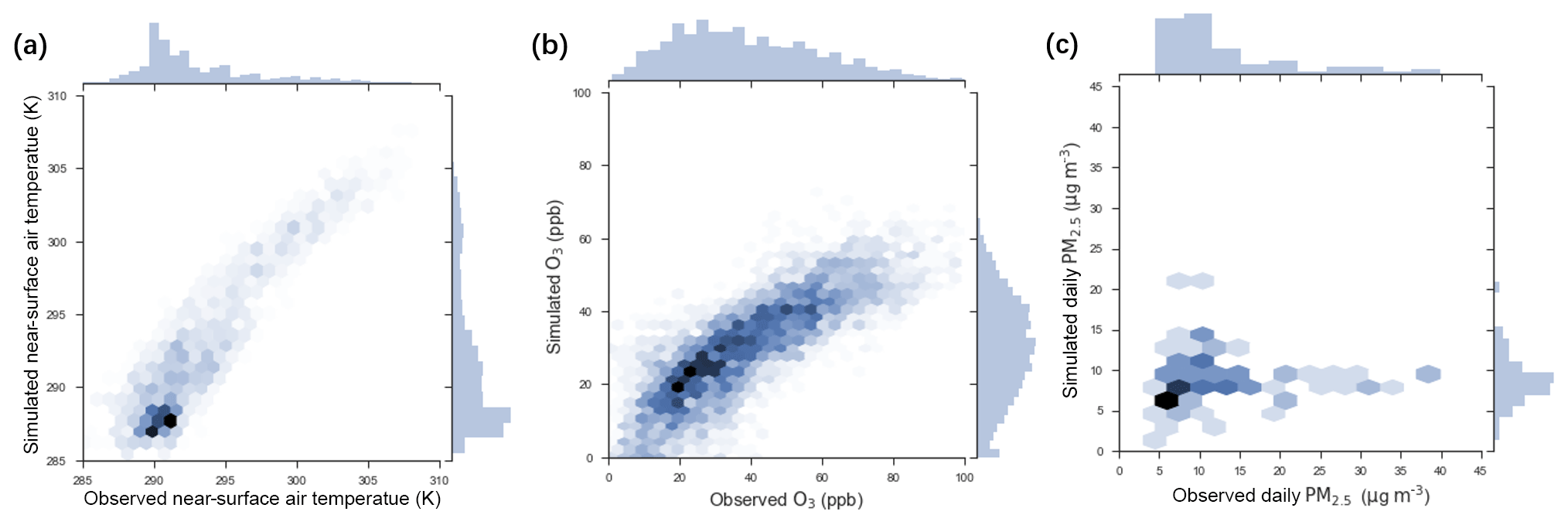
Figure 3Comparison between modeled and observed (a) hourly near-surface air temperature (K), (b) hourly O3 concentrations (ppb), and (c) daily PM2.5 concentrations (µg m−3). Note that daily PM2.5 concentrations from simulations include sea salt but exclude dust. Darker hexagonal bins correspond to higher point densities in the scatter plots. Histograms of both observations and modeled values are also shown at the edges of each panel.
Table 1Summary statistics (mean bias, MB; normalized mean bias, NMB; mean error, ME; and root-mean-square error, RMSE) for model evaluation, which compares modeled (abbreviated as “mod” in the footnote) hourly near-surface air temperature (T2), hourly O3 and daily PM2.5 concentrations to observations (obs).
a Total number of data points comparing modeled versus observed values across all measurement station locations over the simulation period. b . c . d . .
3.2 Effects of urbanization on air temperature and ventilation coefficient
The effects of land surface changes via urbanization in Southern California on air temperature and ventilation coefficient are discussed in this section. Air temperatures are reported for the lowest atmosphere model layer rather than the default diagnostic 2 m (near-surface) air temperature variable to be consistent with reported air pollutant concentrations shown in later sections. (The chemistry code makes use of grid cell air temperature and does not use 2 m air temperature.) Ventilation coefficient is calculated as the product of PBL height and the average wind speed within the PBL and thus considers the combined effects of vertical and horizontal mixing and indicates the ability of the atmosphere to disperse air pollutants (Ashrafi et al., 2009). This calculation can be written as Eq. (1).
where U(zi) stands for horizontal wind speed within the ith model layer (m s−1), Δzi is the depth of the ith model layer that is within the PBL (m), and m is the number of vertical layers up to PBL height.
3.2.1 Spatial average temperature change
As shown in Fig. 4a, our simulations suggest that urbanization in Southern California has in general led to urban temperature reductions during daytime from 07:00 to 16:00 PST and urban temperature increases during other times of day. The largest spatially averaged temperature reduction occurs at 10:00 PST ( K), whereas the largest temperature increase occurs at 20:00 PST (+1.7 K). Additionally, urbanization leads to spatially averaged reduction in diurnal temperature range by 1.5 K. Spatially averaged urban temperature reductions during morning (i.e., defined here and in the following sections as 07:00–12:00 PST) and afternoon (i.e., 12:00–19:00 PST) are −0.9 and −0.3 K, respectively. At nighttime (i.e., 19:00–07:00 PST), the spatially averaged temperature increase is +1.1 K. The spatially averaged changes significantly differ from zero at the 95 % confidence level for all three times of the day using the paired Student's t test with n=7 days.

Figure 4Diurnal cycles for present-day (red), nonurban (blue), and present-day − nonurban (black) for (a) air temperature in the lowest atmospheric layer (K) and (b) ventilation coefficient (m2 s−1). Values are obtained by averaging over urban grid cells and the entire simulation period for each hour of day. The solid and dashed curves give the median values, while the shaded bands show the 25th and 75th percentiles. Dots indicate mean values for differences between present-day and nonurban. The horizontal dotted line in light gray shows Δ=0 as an indicator of positive or negative change by land surface changes via urbanization.
3.2.2 Spatial distributions of temperature change
During the morning, temperature reductions are larger in regions further away from the sea (e.g., San Fernando Valley and Riverside County) than coastal regions (e.g., west Los Angeles and Orange County) (Fig. 5a). (Note that regions that are frequently mentioned in this study are in Fig. 2a.) Spatial patterns in the afternoon are similar to morning, with the exception that coastal regions experience temperature increases (as opposed to decreases) of up to +0.82 K (Fig. 5b). During nighttime, temperature increases spread throughout urban regions and are generally larger in the inland regions of the basin relative to coastal regions (Fig. 5c). A modified version of Fig. 5 that includes values for nonurban cells is in Supplement Fig. S13.
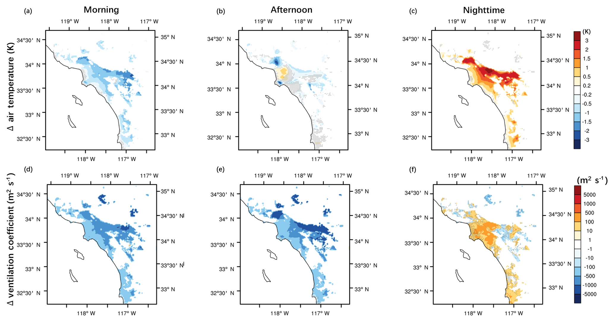
Figure 5Spatial patterns of differences (present-day − nonurban) in temporally averaged values during morning, afternoon, and nighttime for (a, b, c) air temperature in the lowest atmospheric layer and (d, e, f) ventilation coefficient. Morning is defined as 07:00 to 12:00 PST, afternoon as 12:00 to 19:00 PST, and nighttime as 19:00 to 07:00 PST. We refer to morning and afternoon as daytime. Note that values are shown only for urban grid cells. Black dots indicate grid cells where changes are not significantly different from zero at the 95 % confidence level using the paired Student's t test with n=7 days.
3.2.3 Processes driving daytime changes
The temporal and spatial patterns of air temperature changes suggest that the climate response to urbanization during daytime is mainly associated with the competition between (a) temperature reductions from increased evapotranspiration and thermal inertia from urban irrigation and (b) temperature increases from decreased onshore sea breezes (Supplement Fig. S14d, e). Decreases in the onshore sea breeze are primarily caused by increased roughness lengths from urbanization. (Note that the onshore sea breeze decreases in strength despite higher temperatures in the coastal region of Los Angeles during the afternoon, which would tend to increase the land–sea temperature contrast and thus be expected to increase the sea breeze strength.) Inland regions show larger temperature reductions relative to coastal regions because they have lower urban fractions (Fig. S10a in the Supplement), and thus higher pervious fractions. Since irrigation increases soil moisture in the pervious fraction of the grid cell in this model, irrigation will have a larger influence on grid-cell-averaged latent heat fluxes (Fig. S15 in the Supplement) and thermal inertia when pervious fractions are higher. The inland regions are also less affected by changes in the sea breeze relative to coastal regions since they are (a) farther from the ocean and (b) experience smaller increases in roughness length. Roughness length effects on the sea breeze are especially important in the afternoon when baseline wind speeds are generally highest in the Los Angeles basin. Thus, the afternoon temperature increases simulated in the coastal region occur because temperature increases from reductions in the afternoon onshore flows dominate over temperature decreases from increased evapotranspiration. In addition, increases in thermal inertia caused by use of manmade materials (e.g., pavements and buildings) can contribute to simulated temperature reductions during the morning. Please see Supplement Sect. S3 for the additional simulation (present-day no-irrigation scenario) carried out to identify the influence of urbanization but without changing irrigation relative to the nonurban scenario (i.e., with no irrigation).
Note that changes in air temperature during daytime shown here disagree with Vahmani et al. (2016). While our study detects daytime temperature reductions due to urbanization, Vahmani et al. (2016) suggests daytime warming. After detailed comparison of the simulations in our study versus Vahmani et al. (2016), we find that the differences are mainly associated with UCM configuration. First, our study uses model default calculations of surface temperature for the impervious portion of urban grid cells, whereas Vahmani et al. (2016) applied an alternative calculation proposed by Li and Bou-Zeid (2014). Li and Bou-Zeid (2014) intended the alternate surface temperature calculations to be performed as a post-processing step rather than during runtime. After a careful comparison among different model setups, we find that the parameterization of surface temperature is an important factor that affects simulated daytime air temperature (see Fig. S16 in the Supplement). Second, our study accounts for shadow effects in urban canopies, whereas Vahmani et al. (2016) assumes no shadow effects. (We note here that the default version of the UCM has the shadow model turned off. The boolean SHADOW variable in module_sf_urban.F needs to be manually switched to true to enable the shadow model calculations. With the shadow model turned off, all shortwave radiation within the urban canopy is assumed diffuse.) We suggest that it is important to include the effects of building morphology on shadows within the canopy and to track direct and diffuse radiation separately, and we therefore perform simulations in this study with the shadow model on. Note that the effect of shadows is not as significant as the parameterization of surface temperature for most of the domain in our study because the ratio between building height and road width is small.
3.2.4 Processes driving nighttime changes
The climate response to urbanization during nighttime is driven by the combined effects of (a) temperature increases from increasing upward ground heat fluxes and (b) temperature increases from increasing PBL heights. Increased soil moisture (from irrigation) and use of anthropogenic materials leads to higher thermal inertia of the ground; this in turn leads to increased heat storage during the day and higher upward ground heat fluxes and thus surface temperatures at night. Increasing PBL heights can also lead to warming because of lower air cooling rates during nighttime. Changes in PBL heights are associated with surface roughness changes since shear production dominates TKE at night. Coastal (inland) regions show larger (smaller) spatial variation in roughness length (Fig. 2e), which leads to larger (smaller) increases in PBL heights (Fig. S14c in the Supplement). Despite larger increases in PBL heights in coastal versus inland regions, smaller air temperature increases occur in coastal versus inland regions, likely due to accumulative effects from coastal to inland regions with onshore wind flows.
3.2.5 Temporal and spatial patterns of ventilation changes and process drivers
Changes in ventilation coefficient show a similar temporal pattern as air temperature (Fig. 4b); values decrease by up to −36.6 % (equivalent to −826 m2 s−1, at 10:00 PST) during daytime and increase up to +27.0 % (equivalent to +77 m2 s−1, at 23:00 PST) during nighttime, due to urbanization. Absolute reductions in ventilation coefficient are more noticeable in the afternoon than in the morning; the spatially averaged decreases are −726 m2 s−1 (−23 %) and −560 m2 s−1 (−34 %), respectively. These reductions significantly differ from zero at the 95 % confidence level using the paired Student's t test with n=7 days. Reductions during daytime are also generally greater in inland regions than in coastal regions as shown in Fig. 5d and e. Daytime reductions in ventilation occur due to the combined effect of weakened wind speeds due to higher surface roughness and changes (mostly decreases) in PBL heights (Fig. S14 in the Supplement). Changes in PBL heights during daytime are mainly associated with air temperature changes because buoyancy production dominates TKE during the day. Where there are larger air temperature decreases (increases), there is reduced (increased) buoyancy production of TKE, which results in shallower (deeper) PBLs.
At night, spatially averaged ventilation coefficient increases by +8.2 % (+24.3 m2 s−1). This increase significantly differs from zero at the 95 % confidence level. As shown in Fig. 5f, statistically significant ventilation growth occurs in most parts of coastal Los Angeles and Orange County, likely due to higher PBL height increases (i.e., stemming from higher surface roughness increases from urbanization). By contrast, in Riverside County, the effect of reductions in wind speed surpasses changes in PBL heights, leading to slight but not statistically significant reductions in atmospheric ventilation (Fig. S14 in the Supplement).
3.3 Effects of urbanization on NOx and O3 concentrations due to meteorological changes
Concentrations of pollutants are profoundly impacted by meteorological conditions including air temperature and the ventilation capability of the atmosphere (Aw and Kleeman, 2003; Rao et al., 2003). This section discusses how meteorological changes due to land surface changes via urbanization in Southern California affect gaseous pollutant concentrations (i.e., NOx and O3).
3.3.1 Temporal and spatial patterns of NOx concentration changes and process drivers
As shown in Fig. 6a, changes in meteorological fields due to urbanization have led to increases in hourly NOx concentrations during the day (07:00 to 18:00 PST) and decreases at all other times of day. Peak increases in NOx of +2.7 ppb occur at 10:00 PST (i.e., for spatial mean values), while peak decreases of −4.7 ppb occur at 21:00 PST. Spatial mean changes in NOx concentrations are +2.1 and +1.2 ppb in the morning and afternoon, respectively, and −2.8 ppb at night. The spatially averaged changes are significantly different from zero at the 95 % confidence level for all three times of the day. In addition, daily 1 h maximum NOx concentrations change only slightly: from 17.8 ppb at 06:00 PST in the nonurban scenario to 17.9 ppb at 07:00 PST in the present-day scenario.
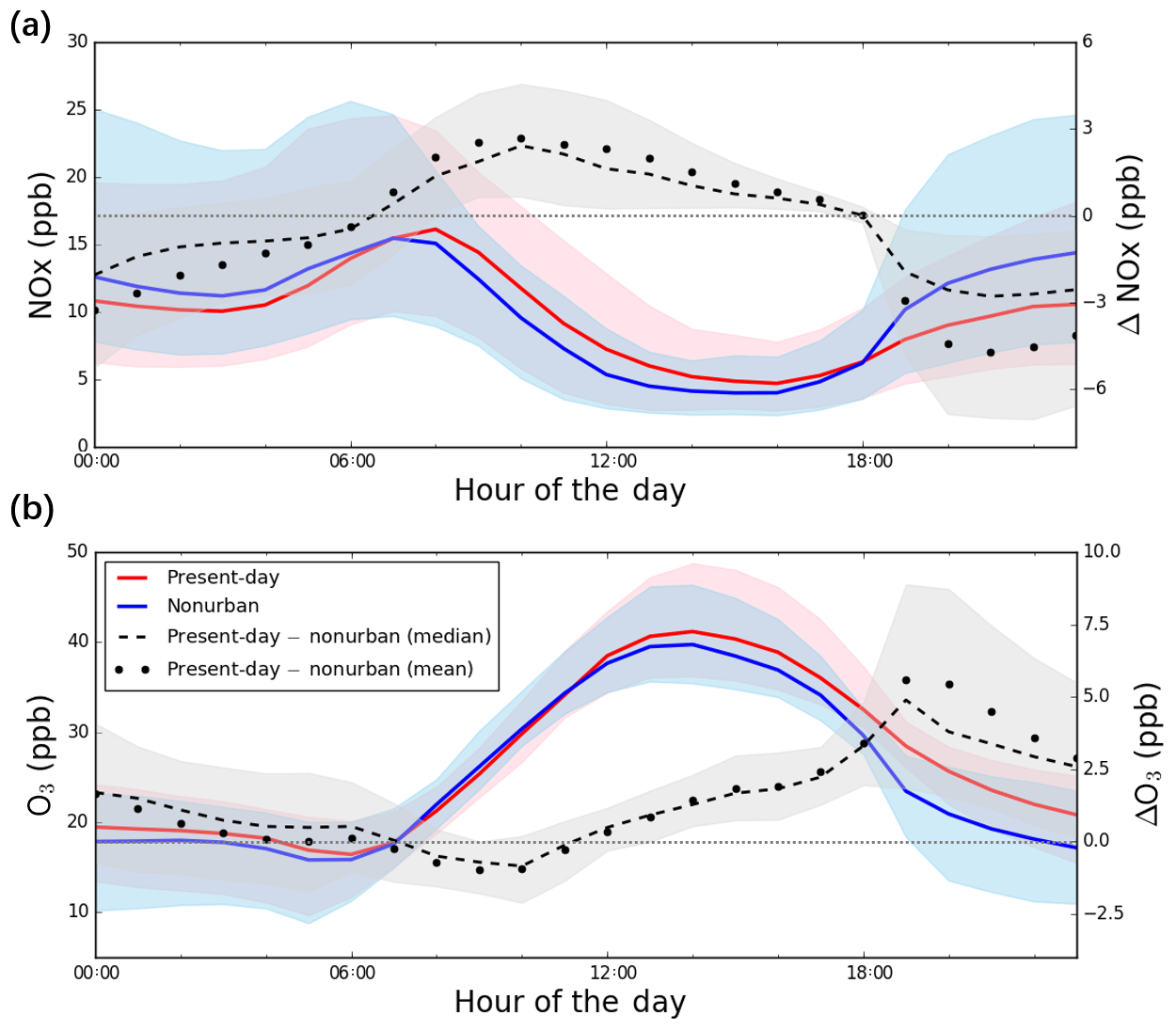
Figure 6Diurnal cycles for present-day (red), nonurban (blue), and present-day − nonurban (black) for (a) NOx (ppb) and (b) O3 concentrations (ppb). Values are obtained by averaging over urban grid cells and the entire simulation period for each hour of day. The solid and dashed curves give the median values, while the shaded bands show the 25th and 75th percentiles. Dots indicate mean values for differences between present-day and nonurban. The horizontal dotted line in light gray shows Δ=0 as an indicator of positive or negative change by land surface changes via urbanization.
Figure 7a, b, c show the spatial patterns of NOx concentration changes due to urbanization. In the morning (afternoon), most inland urban regions show statistically significant increases in NOx concentrations (Fig. 7a, b), with larger NOx concentration increases of up to +13.8 ppb (+5.5 ppb) occurring in inland regions compared to coastal regions. By contrast, NOx concentrations decrease at night across the region, with the largest decreases reaching −20.8 ppb. In general, greater decreases are shown in inland regions compared to coastal regions.
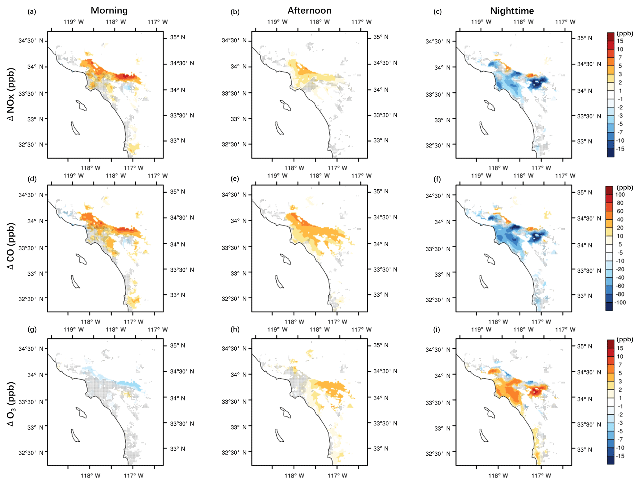
Figure 7Spatial patterns in differences (present-day − nonurban) of temporally averaged values during morning, afternoon, and nighttime for (a, b, c) NOx, (d, e, f) CO, and (g, h, i) O3 concentrations. Morning is defined as 07:00 to 12:00 PST, afternoon as 12:00 to 19:00 PST, and nighttime as 19:00 to 07:00 PST. Black dots indicate grid cells where changes are not significantly different from zero at the 95 % confidence level using the paired Student's t test with n=7 days.
The spatial patterns of changes in NOx concentrations are similar to those for CO concentrations (Fig. 7d, e, f). CO is an inert species and can be used as a tracer for determining the effect of ventilation on air pollutant dispersion since it includes accumulation effects of ventilation changes both spatially and temporally. Thus, the similarity in changes to NOx and CO spatial patterns suggests that NOx changes are driven by ventilation changes. For example, at night, Riverside County shows decreases of up to −20.8 ppb in NOx concentrations (with corresponding decreases in CO of −119 ppb) despite suppressed ventilation at this location because of accumulative effects from coastal to inland regions. A modified version of Fig. 7 that includes values for nonurban cells is in the Supplement Fig. S17.
3.3.2 Temporal and spatial patterns of O3 concentration changes
As indicated by Fig. 6b, O3 concentrations in the lowest atmospheric layer decrease from 07:00 to 11:00 PST and increase during other times of day. The largest decrease of −0.94 ppb occurs at 10:00 PST, while the largest increase of +5.6 ppb occurs at 19:00 PST. Spatially averaged hourly O3 concentrations undergo a −0.6 ppb decrease, +1.7 ppb increase, and +2.1 ppb increase in the morning, afternoon, and night, respectively. The spatially averaged changes significantly differ from zero at the 95 % confidence level for all three times of the day. Additionally, daily 1 h maximum O3 concentrations, which occur at 14:00 PST in both scenarios, increase by +3.4 %, from 41.3 ppb in the nonurban scenario to 42.7 ppb in the present-day scenario. The daily 8 h maximum O3 concentration increases from 38.0 ppb to 39.3 ppb (averaged over 11:00 to 19:00 PST in both scenarios).
Figure 7g, h, i show the spatial patterns of surface O3 concentration changes. In the morning (Fig. 7g), while most regions show reductions in O3 concentrations, the reductions are, in general, statistically insignificant. During the afternoon, most inland urban regions show increases in O3 concentrations (Fig. 7h), with the largest increase of +5.7 ppb occurring in Riverside County. Increases in O3 concentrations are larger during night than the afternoon (Fig. 7i), especially in Riverside County, with the largest increase in O3 concentrations reaching +12.8 ppb.
3.3.3 Processes driving daytime and nighttime changes in O3
The temporal and spatial patterns of changes in O3 concentrations during the day suggest that these changes are mainly driven by the competition between (a) decreases in ventilation, which would tend to cause increases in O3, and (b) the nonlinear response of O3 to NOx changes. In the VOC-limited regime, increases in NOx tend to decrease O3 concentrations, and vice versa. (This explains why decreases in NOx emissions over weekends can cause increases in O3 concentrations, a phenomenon termed the “weekend effect”; Marr and Harley, 2002.) The underlying cause of the weekend effect has to do with titration of O3 by NO, as shown in Reaction (R1).
When NOx is high relative to VOC, Reaction (R1) dominates NO-to-NO2 conversion, which involves consuming O3. In addition, increases in NO2 can reduce OH lifetime due to increased rates of OH + NO2 (Reaction R2), which is chain terminating.
In addition to these two aforementioned processes, changes in air temperature can also affect the production rate of O3, with higher temperatures generally leading to higher O3 (Steiner et al., 2010).
In the morning when ventilation is relatively weak (shallow PBL and weak sea breeze), changes in NOx concentrations play an important role in driving surface O3 concentrations. Regions with greater increases in NOx concentrations in general show greater decreases in O3 concentrations (Fig. 7g). Decreases in air temperature would also contribute to decreases in O3 concentrations due to reductions in O3 production rates. In the afternoon when ventilation is strengthened (deep PBL and stronger sea breeze), changes in both NOx concentrations and ventilation play important roles in determining O3 concentrations (Fig. 7h). Regions with higher increases in NOx concentrations tend to have lower increases in O3 concentrations; this indicates that NOx increases (that would tend to decrease O3) are counteracting decreases in ventilation (that would tend to increase O3). In regions with relatively lower increases in NOx concentrations and greater decreases in ventilation, such as Riverside County, increases in O3 concentrations are larger.
At night, changes in O3 concentrations are dominated by its titration by NO2 as shown in Reaction (R3).
Where there are larger decreases in NOx concentrations (Fig. 7c), there are greater increases in O3 concentrations (Fig. 7i), regardless of the magnitude of increases in atmospheric dilution (Fig. 5f).
3.4 Effects of urbanization on total and speciated PM2.5 concentrations due to meteorological changes
In this section, we discuss changes in total and speciated PM2.5 mass concentrations due to urbanization. Total mass concentrations reported here only consider PM2.5 generated from anthropogenic and biogenic sources mentioned in Sect. 2.3 and exclude sea salt and dust. Speciated PM2.5 is classified into three categories: (secondary) inorganic aerosols including nitrate (), sulfate (), and ammonium (); primary carbonaceous aerosols including elemental carbon (EC) and primary organic carbon (POC); and secondary organic aerosol (SOA) including SOA formed from anthropogenic VOC precursors (ASOA) and biogenic VOC precursors (BSOA).
3.4.1 Temporal patterns of total and speciated PM2.5 concentration changes
Figure 8 illustrates diurnal changes in total and speciated PM2.5 concentrations due to meteorological changes attributable to urbanization. As suggested by Fig. 8a, urbanization is simulated to cause slight spatially averaged increases in total PM2.5 concentrations from 09:00 to 16:00 PST (up to +0.62 µg m−3 occurring at 12:00 PST) and decreases during other times of day (up to −3.1 µg m−3 at 00:00 PST). Increases in total PM2.5 during 09:00 to 16:00 PST come from increases in primary carbonaceous aerosols and nitrate; these species show hourly averaged concentration increases of up to +0.21 and +0.14 µg m−3. By contrast, BSOA decreases slightly during these hours. During other times of day, concentrations of all PM2.5 species decrease dramatically. Inorganic aerosols, primary carbonaceous aerosols, and SOA show decreases of up to −1.7, −0.5, and −0.3 µg m−3, respectively.
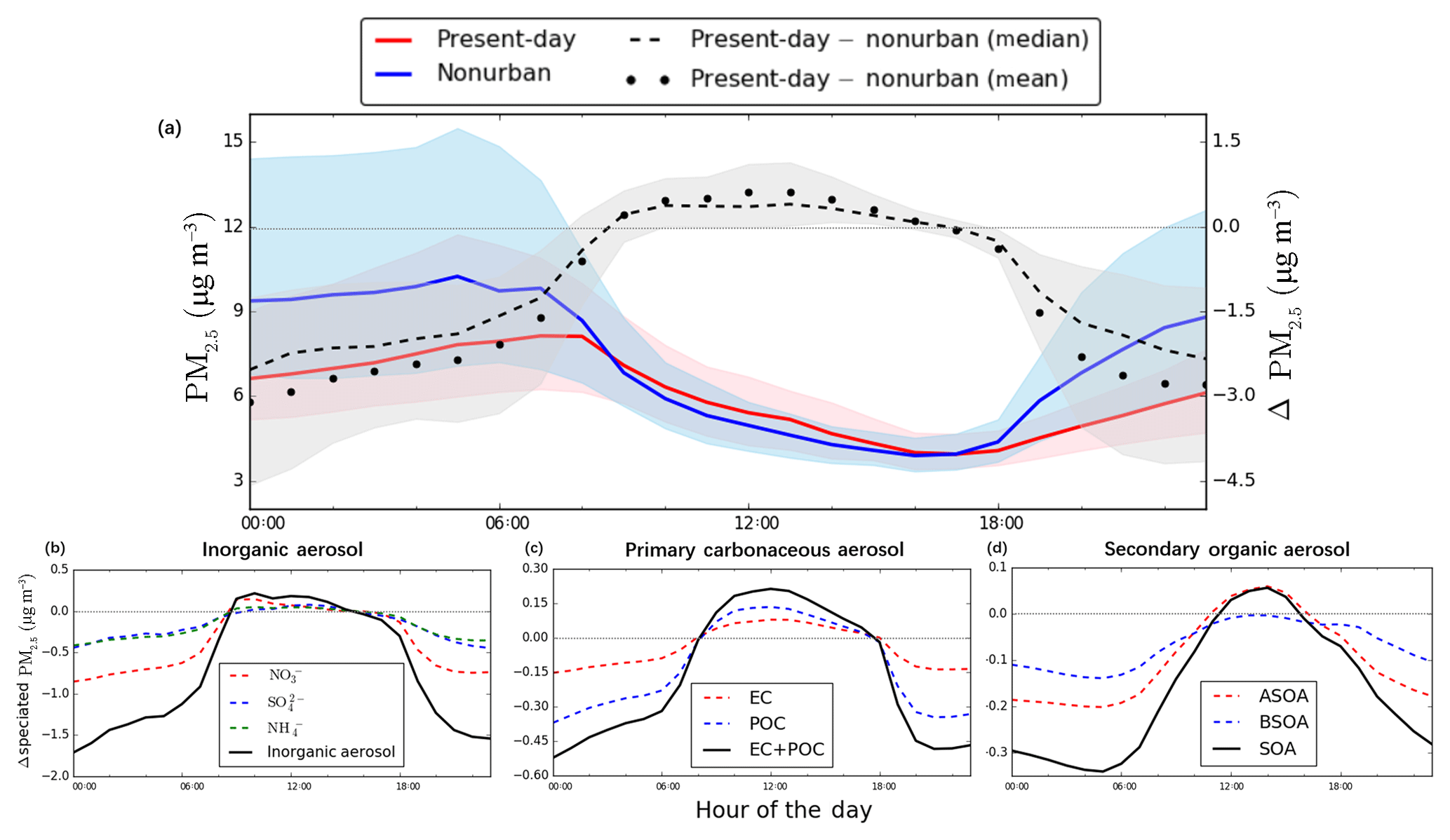
Figure 8Diurnal cycles for spatially averaged PM2.5 concentrations. Panel (a) shows present-day, nonurban, and present-day − nonurban for total PM2.5 (excluding sea salt and dust). Panels (b)–(d) show differences (present-day − nonurban) in speciated PM2.5 including (b) inorganic aerosols (, , ), (c) primary carbonaceous aerosols (EC, POC), and (d) secondary organic aerosols (ASOA, BSOA). The horizontal dotted line in light gray is shown for Δ=0 as an indicator of positive or negative change by urbanization.
During morning hours, averaged hourly total PM2.5 concentrations decrease by −0.20 µg m−3, but the decrease is not statistically significant. In the afternoon, spatially averaged total PM2.5 concentrations increase by +0.24 µg m−3. Primary carbonaceous aerosols contribute to half of the increase (+0.12 µg m−3). For nighttime, total PM2.5 concentrations undergo a decrease of −2.5 µg m−3, with 54 % of the decrease attributed to changes in inorganic aerosols and 17 % to primary carbonaceous aerosols. Both afternoon and nighttime changes are significantly different from zero at the 95 % confidence interval.
3.4.2 Spatial patterns of total and speciated PM2.5 concentration changes
Figure 9 presents spatial patterns of changes in total and speciated PM2.5 due to urbanization. Decreases in concentrations prevail in urban regions during morning and night, whereas increases in concentrations are dominant during the afternoon.
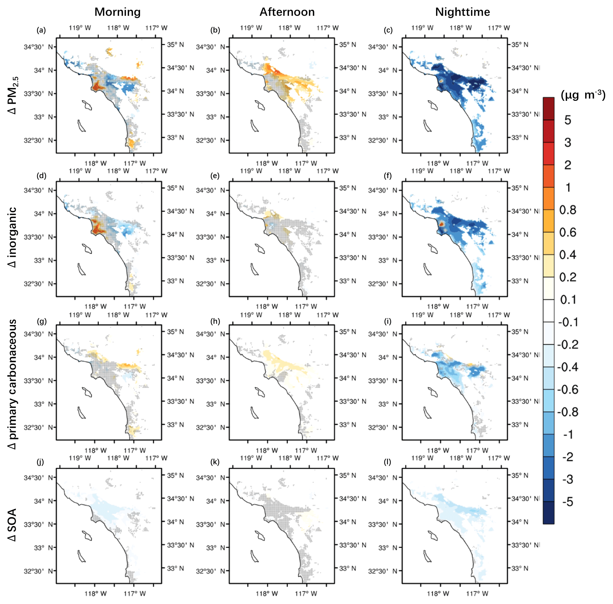
Figure 9Spatial patterns in differences (present-day − nonurban) of temporally averaged values during morning, afternoon, and nighttime for PM2.5. Panels (a)–(c) show total PM2.5, (d)–(f) inorganic aerosol, (g)–(i) primary carbonaceous aerosol, and (j)–(l) secondary organic aerosol. Morning is defined as 07:00 to 12:00 PST, afternoon as 12:00 to 19:00 PST, and nighttime as 19:00 to 07:00 PST. Black dots indicate grid cells where changes are not significantly different from zero at the 95 % confidence level using the paired Student's t test with n=7 days.
In the morning, changes in total PM2.5 and speciated PM2.5 are not statistically distinguishable from zero at the 95 % confidence level. In the afternoon, increases in total PM2.5 are statistically significant in only some inland regions, driven mostly by increases in primary carbonaceous aerosols (up to +0.5 µg m−3, Fig. 9h). At night, most regions within the Los Angeles metropolitan area show decreases in total PM2.5 of −3.0 to −6.0 µg m−3 (Fig. 9c) with contributions from all three categories of speciated PM2.5.
A modified version of Fig. 9 that includes values for nonurban cells is in Supplement Fig. S18.
3.4.3 Processes driving daytime and nighttime changes in PM2.5
During the day, changes in speciated PM2.5 concentrations are dictated by the relative importance of various competing pathways, including (a) reductions in ventilation causing increases in PM2.5, (b) changes in gas–particle phase partitioning causing increases (decreases) in PM2.5 from decreases (increases) in temperature, and (c) increases (decreases) in atmospheric oxidation from increases (decreases) in temperature. Changes in ventilation appear to dominate the changes in primary carbonaceous aerosols, as indicated by the similarity in spatial patterns to changes in CO, which can be considered a conservative tracer (Fig. 7d and e). As for semi-volatile compounds such as nitrate aerosols (red dotted curve in Fig. 8b) and some SOA species, concentrations increase during daytime hours. This is because both decreased ventilation and gas–particle phase partitioning effects favoring the particle phase (from temperature decreases) outweigh reductions in atmospheric oxidation. Concentrations of sulfate and ammonium slightly increase due to urbanization (blue dotted curve in Fig. 8b). Since sulfate is nonvolatile, gas–particle phase partitioning does not affect sulfate concentrations; lowered atmospheric oxidation rates due to reduced temperatures (which would tend to decrease sulfate) nearly offset the effect of weakened ventilation (which would tend to increase sulfate). In addition, BSOA concentrations are simulated to decrease (blue dotted curve in Fig. 8d) due to reduced biogenic VOC emissions, which occur due to reductions in both vegetation coverage and air temperature from urbanization.
At night, decreases in PM2.5 across urban regions are due to (1) enhanced ventilation owing to deeper PBLs (relevant for all PM species) and (2) gas–particle phase partitioning effects that favor the gas phase for semi-volatile compounds (i.e., nitrate aerosols and some SOA species) because of higher air temperatures.
In this study, we have characterized the impact of land surface changes via urbanization on regional meteorology and air quality in Southern California using an enhanced version of WRF–UCM–Chem. We use satellite data for the characterization of land surface properties and include a Southern California-specific irrigation parameterization. The two main simulations of focus in this study are a real-world present-day scenario and a hypothetical nonurban scenario; the former assumes current land cover distributions and irrigation of vegetative areas, while the latter assumes land cover distributions prior to widespread urbanization and no irrigation. We assume identical anthropogenic emissions in these two simulations to allow focus on the effects of land cover change on air pollutant concentrations.
Our results indicate that land surface modifications from historical urbanization have had a profound influence on regional meteorology. Urbanization has led to daytime reductions in air temperature for the lowest model layer and reductions in ventilation within urban areas. The impact of urbanization at nighttime shows the opposite effect, with air temperatures and ventilation coefficients increasing. Spatially averaged reductions in air temperature and ventilation during the day are −0.6 K and −650 m2 s−1, respectively, whereas increases at night are +1.1 K and 24.3 m2 s−1, respectively. Changes in meteorology are spatially heterogeneous; greater changes are simulated in inland regions for (a) air temperature decreases during day and increases during night and (b) ventilation reductions during daytime. Ventilation at night shows increases in coastal areas and decreases in inland areas. Changes in meteorology are mainly attributable to (a) increased surface roughness from buildings, (b) higher evaporative fluxes from irrigation, and (c) higher thermal inertia from building materials and increased soil moisture (from irrigation).
Changes in regional meteorology in turn affect concentrations of gaseous and particulate pollutants. NOx concentrations in the lowest model layer increase by +1.6 ppb during the day and decrease by −2.8 ppb at night, due to changes in atmospheric ventilation. O3 concentrations decrease by −0.6 ppb in the morning and increase by +1.7 (2.2) ppb in the afternoon (night). Decreases in the morning and increases during other times of day are more noticeable in inland regions. Changes in O3 concentrations are mainly attributable to the competition between (a) changes in atmospheric ventilation and (b) changes in NOx concentrations that alter O3 titration. Note that while changes in air temperature can also influence O3 concentrations during the day, this effect is overwhelmed by changes in ventilation and concentrations of NOx in our study. As for PM2.5, total mass concentrations increase by +0.24 µg m−3 in the afternoon and decrease by −2.5 µg m−3 at night. Changes during the morning are not statistically significant. The major driving processes of changes in PM2.5 concentrations are (a) changes in atmospheric ventilation, (b) changes in gas–particle phase partitioning for semi-volatile compounds due to air temperature changes, and (c) changes in atmospheric chemical reaction rates from air temperature changes.
This study highlights the role that land cover properties can have on regional meteorology and air quality. We find that increases in evapotranspiration, thermal inertia, and surface roughness due to historical urbanization are the main drivers of regional meteorology and air quality changes in Southern California. During the day, our simulations suggest that increases in evapotranspiration and thermal inertia from urbanization lead to regional air temperature reductions. Temperature reductions together with increases in surface roughness contribute to decreases in ventilation and consequent increases in ozone and PM2.5 concentrations. During nighttime, increases in thermal inertia from urbanization lead to increases in regional air temperatures. Increases in temperatures together with increase in surface roughness lead to decreases in NOx and PM2.5 concentrations. O3 concentrations increase because of decreased titration by NOx. Our findings indicate that air pollutant concentrations have been impacted by land cover changes since pre-settlement times (i.e., urbanization), even assuming constant anthropogenic emissions. These air pollutant changes are driven by urbanization-induced changes in meteorology. This suggests that policies that impact land surface properties (e.g., urban heat mitigation strategies) can have impacts on air pollutant concentrations (in addition to meteorological impacts); to the extent possible, all environmental systems should be taken into account when studying the benefits or potential penalties of policies that impact the land surface in cities.
The Weather Research and Forecasting Model can be downloaded at http://www2.mmm.ucar.edu/wrf/users/download/get_sources.html (last access: 25 March 2019). Other datasets are publicly available as cited. Raw model outputs are TB file sizes and thus not publicly available, but processed data may be available by contacting the authors.
The supplement related to this article is available online at: https://doi.org/10.5194/acp-19-4439-2019-supplement.
GABW designed the study. YL performed the model simulations, carried out data analysis, and wrote the paper. GABW and DJS mentored YL. JZ contributed to the setup of WRF–UCM–Chem. All authors contributed to editing the paper.
The authors declare that they have no conflict of interest.
This research is supported by the US National Science Foundation under grants CBET-1512429, CBET-1623948, and CBET-1752522. Model simulations for the work described in this paper are supported by the University of Southern California's Center for High-Performance Computing (https://hpcc.usc.edu/, last access: 14 July 2018). We thank Scott Epstein and Sang-Mi Lee at the South Coast Air Quality Management District and Jeremy Avise at California Air Resources Board for providing us emission datasets. We also thank Ravan Ahmadov and Stu McKeen at the National Oceanic and Atmospheric Administration for their helpful suggestions.
This paper was edited by Robert Harley and reviewed by three anonymous referees.
Abdul-Wahab, S. A., Bakheit, C. S., and Al-Alawi, S. M.: Principal component and multiple regression analysis in modelling of ground-level ozone and factors affecting its concentrations, Environ. Modell. Softw., 20, 1263–1271, 2005.
Ackermann, I. J., Hass, H., Memmesheimer, M., Ebel, A., Binkowski, F. S., and Shankar, U.: Modal aerosol dynamics model for Europe: development and first applications, Atmos. Environ., 32, 2981–2999, 1998.
Ahmadov, R., McKeen, S. A., Robinson, A. L., Bahreini, R., Middlebrook, A. M., de Gouw, J. A., Meagher, J., Hsie, E.-Y., Edgerton, E., Shaw, S., and Trainer, M.: A volatility basis set model for summertime secondary organic aerosols over the eastern United States in 2006, J. Geophys. Res.-Atmos., 117, D06301, https://doi.org/10.1029/2011JD016831, 2012.
American Lung Association: State of the Air 2012, available at: http://www.stateoftheair.org/2012/assets/state-of-the-air2012.pdf (last access: 12 March 2018), 2012.
Ashrafi, K., Shafie-Pour, and Kamalan, H.: Estimating Temporal and Seasonal Variation of Ventilation Coefficients, Int. J. Environ. Res, 3, 637–644, 2009.
Aw, J. and Kleeman, M. J.: Evaluating the first-order effect of intraannual temperature variability on urban air pollution, J. Geophys. Res., 108, 4365, https://doi.org/10.1029/2002JD002688, 2003.
Boucher, O., Randall, D., Artaxo, P., Bretherton, C., Feingold, G., Forster, P., Kerminen, V.-M., Kondo, Y., Liao, H., Lohmann, U., Rasch, P., Satheesh, S. K., Sherwood, S., Stevens, B. and Zhang, X. Y.: Clouds and Aerosols, in: Climate Change 2013: The Physical Science Basis, in: Contribution of Working Group I to the Fifth Assessment Report of the Intergovernmental Panel on Climate Change, edited by: Stocker, T. F., Qin, D., Plattner, G.-K., Tignor, M., Allen, S. K., Boschung, J., Nauels, A., Xia, Y., Bex, V., and Midgley, P. M., Cambridge University Press, Cambridge, UK and New York, NY, USA, 571–657, 2013.
Burian, S. J. and Shepherd, J. M.: Effect of urbanization on the diurnal rainfall pattern in Houston, Hydrol. Process., 19, 1089–1103, 2005.
CARB: ARB's Emission Inventory Activities, available at: https://www.arb.ca.gov/ei/ei.htm, last access: 10 June 2017.
Carnahan, W. H. and Larson, R. C.: An analysis of an urban heat sink, Remote Sens. Environ., 33, 65–71, 1990.
Carter, W. P. L.: The SAPRC-99 Chemical Mechanism and Updated VOC Reactivity Scales, available at: http://www.engr.ucr.edu/~carter/reactdat.htm, 2003.
Charlson, R. J., Schewartz, S. E., Hales, J. M., Cess, R. D., Coarley J. A., J., Hansen, J. E., and Hofmann, D. J.: Climate Forcing by Anthropogenic Aerosols, Science, 255, 423–430, 1992.
Chen, F. and Dudhia, J.: Coupling an Advanced Land Surface–Hydrology Model with the Penn State – NCAR MM5 Modeling System. Part I: Model Implementation and Sensitivity, Mon. Weather Rev., 129, 569–585, 2001.
Chen, F., Kusaka, H., Bornstein, R., Ching, J., Grimmond, C. S. B., Grossman-Clarke, S., Loridan, T., Manning, K. W., Martilli, A., Miao, S., Sailor, D., Salamanca, F. P., Taha, H., Tewari, M., Wang, X., Wyszogrodzki, A. A., and Zhang, C.: The integrated WRF/urban modelling system: development, evaluation, and applications to urban environmental problems, Int. J. Climatol., 31, 273–288, 2011.
Chen, L., Zhang, M., Zhu, J., Wang, Y., and Skorokhod, A.: Modeling Impacts of Urbanization and Urban Heat Island Mitigation on Boundary Layer Meteorology and Air Quality in Beijing Under Different Weather Conditions, J. Geophys. Res.-Atmos., 123, 4323–4344, 2018.
Ching, J., Brown, M., McPherson, T., Burian, S., Chen, F., Cionco, R., Hanna, A., Hultgren, T., McPherson, T., Sailor, D., Taha, H., and Williams, D.: National Urban Database and Access Portal Tool, B. Am. Meteorol. Soc., 90, 1157–1168, 2009.
Chou, M.-D. and Suarez, M. J.: Technical Report Series on Global Modeling and Data Assimilation, Volume 15, in: A Solar Radiation Parameterization for Atmospheric Studies, Goddard Space Flight Center, Greenbelt, MD, USA, 1–38, 1999.
Civerolo, K., Hogrefe, C., Lynn, B., Rosenthal, J., Ku, J.-Y., Solecki, W., Cox, J., Small, C., Rosenzweig, C., Goldberg, R., Knowlton, K., and Kinney, P.: Estimating the Effects of Increased Urbanization on Surface Meteorology and Ozone Concentrations in the New York City Metropolitan Region, Atmos. Environ., 41, 1803–1818, 2007.
Dyer, A. J. and Hicks, B. B.: Flux-gradient Relationships in the Constant Flux Layer, Q. J. Meteor. Soc., 96, 715–721, 1970.
Epstein, S. A., Lee, S.-M., Katzenstein, A. S., Carreras-Sospedra, M., Zhang, X., Farina, S. C., Vahmani, P., Fine, P. M., Ban-Weiss, G.: Air-quality Implications of Widespread Adoption of Cool Roofs on Ozone and Particulate Matter in Southern California, P. Natl. Acad. Sci. USA, 114, 8991–8996, 2017.
Fallmann, J., Forkel, R., and Emeis, S.: Secondary Effects of Urban Heat Island Mitigation Measures on Air Quality, Atmos. Environ., 125, 199–211, 2016.
Fan, C., Myint, S., Kaplan, S., Middel, A., Zheng, B., Rahman, A., Huang, H.-P., Brazel, A., and Blumberg, D. G.: Understanding the Impact of Urbanization on Surface Urban Heat Islands – A Longitudinal Analysis of the Oasis Effect in Subtropical Desert Cities, Remote Sens., 9, 672, 2017.
Fry, J., Xian, G. Z., Jin, S., Dewitz, J., Homer, C. G., Yang, L., Barnes, C. A., Herold, N. D., and Wickham, J. D.: Completion of the 2006 National Land Cover Database for the Conterminous United States, Photogramm. Eng. Remote Sens., 77, 858–864, 2011.
Garratt, J. R.: The Atmospheric Boundary Layer, edited by: Houghton, J. T., Rycroft, M. J., and Dessler, A. J., Cambridge University Press, Cambridge, UK, 15–38, 1994.
Georgescu, M., Morefield, P. E., Bierwagen, B. G., and Weaver, C. P.: Urban Adaptation can Roll Back Warming of Emerging Megapolitan Regions, P. Natl. Acad. Sci. USA, 111, 2909–2914, 2014.
Grell, G. A. and Dévényi, D.: A Generalized Approach to Parameterizing Convection Combining Ensemble and Data Assimilation Techniques, Geophys. Res. Lett., 29, 38-1–38-4, 2012.
Grell, G. A., Peckham, S. E., Schmitz, R., McKeen, S. A., Frost, G., Skamarock, W. C., and Eder, B.: Fully Coupled “Online” Chemistry within the WRF Model, Atmos. Environ., 39, 6957–6975, 2005.
Grimm, N. B., Faeth, S. H., Golubiewski, N. E., Redman, C. L., Wu, J., Bai, X., and Briggs, J. M.: Global Change and the Ecology of Cities, Science, 319, 756–760, 2008.
Guenther, A., Karl, T., Harley, P., Wiedinmyer, C., Palmer, P. I., and Geron, C.: Estimates of global terrestrial isoprene emissions using MEGAN (Model of Emissions of Gases and Aerosols from Nature), Atmos. Chem. Phys., 6, 3181–3210, https://doi.org/10.5194/acp-6-3181-2006, 2006.
Hardin, A. W. and Vanos, J. K.: The Influence of Surface Type on the Absorbed Radiation by a Human Under Hot, Dry Conditions, Int. J. Biometeorol., 62, 43–56, 2018.
Hassan, S. K., El–Abssawy, A. A., and Khoder, M. I.: Characteristics of Gas–Phase Nitric Acid and Ammonium–Nitrate–Sulfate Aerosol, and Their Gas–Phase Precursors in a Suburban Area in Cairo, Egypt, Atmos. Pollut. Res., 4, 117–129, 2013.
Hong, S.-Y., Noh, Y., Dudhia, J., Hong, S.-Y., Noh, Y., and Dudhia, J.: A New Vertical Diffusion Package with an Explicit Treatment of Entrainment Processes, Mon. Weather Rev., 134, 2318–2341, 2016.
Imhoff, M. L., Zhang, P., Wolfe, R. E., and Bounoua, L.: Remote Sensing of the Urban Heat Island Effect Across Biomes in the Continental USA, Remote Sens. Environ., 114, 504–513, 2010.
Jiang, X., Wiedinmyer, C., Chen, F., Yang, Z.-L., and Lo, J. C.-F.: Predicted Impacts of Climate and Land Use Change on Surface Ozone in the Houston, Texas, Area, J. Geophys. Res., 113, D20312, https://doi.org/10.1029/2008JD009820, 2008.
Kalnay, E. and Cai, M.: Impact of Urbanization and Land-Use Change on Climate, Nature, 423, 528–531, 2003.
Kim, S.-W., Heckel, A., Frost, G. J., Richter, A., Gleason, J., Burrows, J. P., McKeen, S., Hsie, E.-Y., Granier, C., and Trainer, M.: NO2 Columns in the Western United States Observed from Space and Simulated by a Regional Chemistry Model and Their Implications for NOx Emissions, J. Geophys. Res., 114, D11301, https://doi.org/10.1029/2008JD011343, 2009.
Kumar, R., Mishra, V., Buzan, J., Kumar, R., Shindell, D., and Huber, M.: Dominant Control of Agriculture and Irrigation on Urban Heat Island in India, Sci. Rep.-UK, 7, 14054, https://doi.org/10.1038/s41598-017-14213-2, 2017.
Kusaka, H., Chen, F., Tewari, M., Dudhia, J., Gill, D. O., Duda, M. G., Wang, W., and Miya, I. Y.: Numerical Simulation of Urban Heat Island Effect by the WRF Model with 4-km Grid Increment: An Inter-Comparison Study between the Urban Canopy Model and Slab Model, J. Meteorol. Soc. Jpn. Ser. II, 90B, 33–45, 2012.
Kusaka, H., Kondo, H., Kikegawa, Y., and Kimura, F.: A Simple Single-Layer Urban Canopy Model For Atmospheric Models: Comparison With Multi-Layer And Slab Models, Bound.-Lay. Meteorol., 101, 329–358, 2001.
Li, D. and Bou-Zeid, E.: Quality and Sensitivity of High-Resolution Numerical Simulation of Urban Heat Islands, Environ. Res. Lett., 9, 055001, https://doi.org/10.1088/1748-9326/9/5/055001, 2014.
Li, M., Wang, T., Xie, M., Zhuang, B., Li, S., Han, Y., Song, Y., and Cheng, N.: Improved Meteorology and Ozone Air Quality Simulations Using MODIS Land Surface Parameters in the Yangtze River Delta Urban Cluster, China, J. Geophys. Res.-Atmos., 122, 3116–3140, 2017.
Lin, Y.-L., Farley, R. D., Orville, H. D., Lin, Y.-L., Farley, R. D., and Orville, H. D.: Bulk Parameterization of the Snow Field in a Cloud Model, J. Clim. Appl. Meteorol., 22, 1065–1092, 1983.
Lippmann, M.: Health Effects of Ozone: A Critical Review, J. Air Waste Manage., 39, 672–695, 1989.
Madronich, S.: Photodissociation in the Atmosphere: 1. Actinic Flux and the Effects of Ground Reflections and Clouds, J. Geophys. Res., 92, 9740, https://doi.org/10.1029/JD092iD08p09740, 1987.
Marr, L. C. and Harley, R. A.: Spectral Analysis of Weekday–Weekend Differences in Ambient Ozone, Nitrogen Oxide, and Non-Methane Hydrocarbon Time Series in California, Atmos. Environ., 36, 2327–2335, 2002.
Mesinger, F., DiMego, G., Kalnay, E., Mitchell, K., Shafran, P. C., Ebisuzaki, W., Jović, D., Woolen, J., Rogers, E., Berbery, E. H., Ek, M. B., Fan, Y., Grumbine, R., Higgins, W., Li, H., Lin, Y., Manikin, G., Parrish, D., and Shi, W.: North American Regional Reanalysis, B. Am. Meteorol. Soc., 87, 343–360, 2006.
Mlawer, E. J., Taubman, S. J., Brown, P. D., Iacono, M. J., and Clough, S. A.: Radiative Transfer for Inhomogeneous Atmospheres: RRTM, a Validated Correlated-k Model for the Longwave, J. Geophys. Res.-Atmos., 102, 16663–16682, 1997.
Oke, T. R.: The Energetic Basis of the Urban Heat Island, Q. J. Roy. Meteorol. Soc., 108, 1–24, 1982.
Pankow, J. F.: Partitioning of Semi-Volatile Organic Compounds to the Air/Water Interface, Atmos. Environ., 31, 927–929, 1997.
Paulson, C. A.: The Mathematical Representation of Wind Speed and Temperature Profiles in the Unstable Atmospheric Surface Layer, J. Appl. Meteorol., 9, 857–861, 1970.
Peng, S., Piao, S., Ciais, P., Friedlingstein, P., Ottle, C., Breón, F. O.-M., Nan, H., Zhou, L., and Myneni, R. B.: Surface Urban Heat Island Across 419 Global Big Cities, Environ. Sci. Technol., 46, 696–703, 2012.
Pope, C. A. and Dockery, D. W.: Health Effects of Fine Particulate Air Pollution: Lines that Connect, J. Air Waste Ma., 56, 709–742, 2006.
Qiao, Z., Tian, G., and Xiao, L.: Diurnal and Seasonal Impacts of Urbanization on the Urban Thermal Environment: A Case Study of Beijing Using MODIS Data, ISPRS J. Photogramm., 85, 93–101, 2013.
Rao, S. T., Ku, J. Y., Berman, S., Zhang, K., and Mao, H.: Summertime Characteristics of the Atmospheric Boundary Layer and Relationships to Ozone Levels over the Eastern United States, Pure Appl. Geophys., 160, 21–55, 2003.
Rizwan, A. M., Dennis, L. Y. C., and Liu, C.: A Review on the Generation, Determination and Mitigation of Urban Heat Island, J. Environ. Sci., 20, 120–128, 2008.
SCAQMD: Final 2016 Air Quality Management Plan, Appendix III: Base and Future Year Emission Inventory, available at: http://www.aqmd.gov/docs/default-source/clean-air-plans/air-quality-management-plans/2016-air-quality-management-plan/final-2016-aqmp/appendix-iii.pdf (last access: 10 March 2018), 2017.
Seto, K. C., Güneralp, B., and Hutyra, L. R.: Global Forecasts of Urban Expansion to 2030 and Direct Impacts on Biodiversity and Carbon Pools, P. Natl. Acad. Sci. USA, 109, 16083–16088, 2012.
Steiner, A. L., Davis, A. J., Sillman, S., Owen, R. C., Michalak, A. M., and Fiore, A. M.: Observed Suppression of Ozone Formation at Extremely High Temperatures due to Chemical and Biophysical Feedbacks, P. Natl. Acad. Sci. USA, 107, 19685–19690, 2010.
Stewart, I. D. and Oke, T. R.: Local Climate Zones for Urban Temperature Studies, B. Am. Meteorol. Soc., 93, 1879–1900, 2012.
Stockwell, W. R., Kirchner, F., Kuhn, M., and Seefeld, S.: A New Mechanism for Regional Atmospheric Chemistry Modeling, J. Geophys. Res.-Atmos., 102, 25847–25879, 1997.
Stockwell, W. R., Middleton, P., Chang, J. S., and Tang, X.: The Second Generation Regional Acid Deposition Model Chemical Mechanism for Regional Air Quality Modeling, J. Geophys. Res., 95, 16343, https://doi.org/10.1029/JD095iD10p16343, 1990.
Taha, H.: Meteorological, Air-Quality, and Emission-Equivalence Impacts of Urban Heat Island Control in California, Sustain. Cities Soc., 19, 207–221, 2015.
Tao, W., Liu, J., Ban-Weiss, G. A., Hauglustaine, D. A., Zhang, L., Zhang, Q., Cheng, Y., Yu, Y., and Tao, S.: Effects of urban land expansion on the regional meteorology and air quality of eastern China, Atmos. Chem. Phys., 15, 8597–8614, https://doi.org/10.5194/acp-15-8597-2015, 2015.
Theeuwes, N. E., Steeneveld, G.-J., Ronda, R. J., Rotach, M. W., and Holtslag, A. A. M.: Cool City Mornings by Urban Heat, Environ. Res. Lett., 10, 114022, https://doi.org/10.1088/1748-9326/10/11/114022, 2015.
US EPA: Profile of the 2011 National Air Emissions Inventory, available at: https://www.epa.gov/sites/production/files/2015-08/documents/lite_finalversion_ver10.pdf (last access: 10 March 2018), 2014.
Vahmani, P. and Ban-Weiss, G. A.: Impact of Remotely Sensed Albedo and Vegetation Fraction on Simulation of Urban Climate in WRF-Urban Canopy Model: A Case Study of the Urban Heat Island in Los Angeles, J. Geophys. Res.-Atmos., 121, 1511–1531, 2016a.
Vahmani, P. and Ban-Weiss, G.: Climatic Consequences of Adopting Drought-Tolerant Vegetation Over Los Angeles as a Response to California Drought, Geophys. Res. Lett., 43, 8240–8249, 2016b.
Vahmani, P. and Hogue, T. S.: Incorporating an Urban Irrigation Module into the Noah Land Surface Model Coupled with an Urban Canopy Model, J. Hydrometeorol., 15, 1440–1456, 2014.
Vahmani, P., Sun, F., Hall, A., and Ban-Weiss, G.: Investigating the Climate Impacts of Urbanization and the Potential for Cool Roofs to Counter Future Climate Change in Southern California, Environ. Res. Lett., 11, 124027, https://doi.org/10.1088/1748-9326/11/12/124027, 2016.
Wang, K., Jiang, S., Wang, J., Zhou, C., Wang, X., and Lee, X.: Comparing the Diurnal and Seasonal Variabilities of Atmospheric and Surface Urban Heat Islands Based on the Beijing Urban Meteorological Network, J. Geophys. Res.-Atmos., 122, 2131–2154, 2017.
Wesely, M. L.: Parameterization of Surface Resistances to Gaseous Dry Deposition in Regional-Scale Numerical Models, Atmos. Environ., 23, 1293–1304, 1989.
Wickham, J. D., Stehman, S. V., Gass, L., Dewitz, J., Fry, J. A., and Wade, T. G.: Accuracy Assessment of NLCD 2006 Land Cover and Impervious Surface, Remote Sens. Environ., 130, 294–304, 2013.
Xu, M., Chang, C.-P., Fu, C., Qi, Y., Robock, A., Robinson, D., and Zhang, H.: Steady Decline of East Asian Monsoon Winds, 1969–2000: Evidence from Direct Ground Measurements of Wind Speed, J. Geophys. Res., 111, D24111, https://doi.org/10.1029/2006JD007337, 2006.
Yang, J., Wang, Z.-H., Chen, F., Miao, S., Tewari, M., Voogt, J. A., and Myint, S.: Enhancing Hydrologic Modelling in the Coupled Weather Research and Forecasting–Urban Modelling System, Bound.-Lay. Meteorol., 155, 87–109, 2015.
Zhang, J., Mohegh, A., Li, Y., Levinson, R., and Ban-Weiss, G.: Systematic Comparison of the Influence of Cool Wall Versus Cool Roof Adoption on Urban Climate in the Los Angeles Basin, Environ. Sci. Technol., 52, 11188–11197, 2018a.
Zhang, J., Li, Y., Tao, W., Liu, J., Levinson, R., Mohegh, A., and Ban-Weiss., G.: Investigating the Urban Air Quality Effects of Cool Walls and Cool Roofs in Southern California, submitted, Environ. Sci. Technol., 2018b.
Zhang, N., Gao, Z., Wang, X., and Chen, Y.: Modeling the Impact of Urbanization on the Local and Regional Climate in Yangtze River Delta, China, Theor. Appl. Climatol., 102, 331–342, 2010.
Zhao, L., Lee, X., Smith, R. B., and Oleson, K.: Strong Contributions of Local Background Climate to Urban Heat Islands, Nature, 511, 216–219, 2014.