the Creative Commons Attribution 4.0 License.
the Creative Commons Attribution 4.0 License.
 | 19 Mar 2019
Development of a unit-based industrial emission inventory in the Beijing–Tianjin–Hebei region and resulting improvement in air quality modeling
Haotian Zheng
Siyi Cai
Xing Chang
Jiming Hao
The Beijing–Tianjin–Hebei (BTH) region is a metropolitan area with the most severe fine particle (PM2.5) pollution in China. An accurate emission inventory plays an important role in air pollution control policy making. In this study, we develop a unit-based emission inventory for industrial sectors in the BTH region, including power plants, industrial boilers, steel, non-ferrous metal smelting, coking plants, cement, glass, brick, lime, ceramics, refineries, and chemical industries, based on detailed information for each enterprise, such as location, annual production, production technology/processes, and air pollution control facilities. In the BTH region, the emissions of sulfur dioxide (SO2), nitrogen oxide (NOx), particulate matter with diameter less than 10 µm (PM10), PM2.5, black carbon (BC), organic carbon (OC), and non-methane volatile organic compounds (NMVOCs) from industrial sectors were 869, 1164, 910, 622, 71, 63, and 1390 kt in 2014, respectively, accounting for a respective 61 %, 55 %, 62 %, 56 %, 58 %, 22 %, and 36 % of the total emissions. Compared with the traditional proxy-based emission inventory, much less emissions in the high-resolution unit-based inventory are allocated to the urban centers due to the accurate positioning of industrial enterprises. We apply the Community Multi-scale Air Quality (CMAQ; version 5.0.2) model simulation to evaluate the unit-based inventory. The simulation results show that the unit-based emission inventory shows better performance with respect to both PM2.5 and gaseous pollutants than the proxy-based emission inventory. The normalized mean biases (NMBs) are 81 %, 21 %, 1 %, and −7 % for the concentrations of SO2, NO2, ozone (O3), and PM2.5, respectively, with the unit-based inventory, in contrast to 124 %, 39 %, −8 %, and 9 % with the proxy-based inventory; furthermore, the concentration gradients of PM2.5, which are defined as the ratio of the urban concentration to the suburban concentration, are 1.6, 2.1, and 1.5 in January and 1.3, 1.5, and 1.3 in July, for simulations with the unit-based inventory, simulations with the proxy-based inventory, and observations, respectively, in Beijing. For O3, the corresponding gradients are 0.7, 0.5, and 0.9 in January and 0.9, 0.8, and 1.1 in July, implying that the unit-based emission inventory better reproduces the distributions of pollutant emissions between the urban and suburban areas.
- Article
(10183 KB) - Full-text XML
-
Supplement
(1446 KB) - BibTeX
- EndNote


The Beijing–Tianjin–Hebei (BTH) region is the political, economic, and cultural center of China. According to China National Environmental Monitoring Centre (2018), in 2017, the annual average concentrations of PM2.5 in Beijing, Tianjin, and Hebei were 65.6, 63.8, and 57.1 µg m−3, respectively, ranking them second, third and sixth among all provinces. The severe PM2.5 pollution in the BTH region is largely attributed to the substantial emissions of air pollutants (B. Zhao et al., 2017). An accurate emission inventory, in terms of both emission rates and spatial distribution, is imperative for an adequate understanding of the sources and the formation mechanism of serious air pollution in this area.
The spatial distribution is one of the most uncertain components of emission inventories considering the diverse source categories and complex emission characteristics. The traditional method of spatial allocation is to distribute the emissions by administrative region into grids based on spatial proxies such as population, gross domestic product (GDP), road map, land use data, and nighttime lights (Geng et al., 2017; Oda and Maksyutov, 2011; Streets et al., 2003). The results may deviate significantly from the actual spatial distributions of many sources (Zhou and Gurney, 2011), especially the power and industrial sources, which contribute over 50 % of the total PM2.5 emissions in China (Zhao et al., 2013a). Due to the stricter air quality regulations and the higher land prices in urban areas, people tend to build factories in suburban areas where the population density and GDP are lower. Zheng et al. (2017) studied the influence of the resolution of gridded emission inventories and found that there were large biases when the inventories were distributed to very fine resolutions following the traditional proxy-based allocation method. The emission inventory could be significantly improved with detailed information regarding point sources such as power plants, steel plants, and cement plants. The high spatial resolution of the inventory may subsequently improve the air quality modeling results and enable a better source apportionment of air pollution (Y. Zhao et al., 2017).
A number of studies have developed the emission inventory in the BTH region (Li et al., 2017; Wang et al., 2014), whereas others have provided emission estimates for this region as part of national or larger-scale emission inventories (Ohara et al., 2007; Stohl et al., 2015). However, only limited studies have estimated the emissions from individual point sources (i.e., a unit-based emission inventory). Zhao et al. (2008), Chen et al. (2014), and Liu et al. (2015) established unit-based emission inventories of coal-fired power plants in China. K. Wang et al. (2016) and Wu et al. (2015) developed an emission inventory for the steel industry. Lei et al. (2011) and Chen et al. (2015) established an emission inventory for the cement industry in China. Qi et al. (2017) established an emission inventory in the BTH region in which power and major industrial sources were treated as point sources. These studies usually focused on one or several major industries, and did not cover all industrial sectors in the BTH region. Moreover, these previous studies seldom validated the unit-based emission inventory or evaluated the improvement it brings to air quality simulation.
In this study, we developed a unit-based emission inventory of industrial sectors for the BTH region. A three-domain nested simulation by the WRF-CMAQ (Weather Research and Forecasting–Community Multi-scale Air Quality) model was applied to evaluate the emission inventory. In order to study the influence of the point sources, we compared the simulation results of this emission inventory with those of a traditional proxy-based emission inventory.
2.1 High-resolution emission inventory for the BTH region
A unit-based method is applied to quantify the emissions from industrial sectors such as power plants, industrial boilers, iron and steel production, non-ferrous metal smelters, coking plants, cement, glass, brick, lime, ceramics, refineries, and chemical industries in 2014. The product yields used for estimating emissions of each sector are shown in Table S4 in the Supplement. The pollutant emissions from each industrial enterprise are calculated from activity level (energy consumption for power plants and industrial boilers, and product yield for other sectors), the emission factor, and the removal efficiency of control technology, as shown in the following equation:
where Ei,j is emissions of pollutant i from industrial enterprise j, Aj is the activity level of industrial enterprise j, EFi,j is the uncontrolled emission factor of pollutant i from industrial enterprise j, and ηi,j is the removal efficiency of pollutant i by control technology in enterprise j. ηi,j is determined by the production process and control technology of the industrial enterprise. The EFi,j values, which depend on the production process of the industrial enterprise, are calculated according to the sulfur and ash contents of fuels, e.g., coal, used in each province (for PM and SO2), or obtained from our previous study (Zhao et al., 2013b), for other pollutants.
Some industrial sources involve multiple production processes, such as iron and steel production and cement production. Using cement production as an example, emissions are calculated using the following equation:
where Ei,j values are the emissions of pollutant i from industrial enterprise j, AKj,m is the amount of clinker produced by the clinker burning process m of the enterprise j, EFi,m is the uncontrolled emission factor for pollutant i from the clinker burning process m, is the removal efficiency of pollutant i from the clinker burning process m in enterprise j, ACj is the amount of cement produced by enterprise j, efi values are the uncontrolled emission factors from the clinker processing stage (efi=0 if i is not particulate matter), ηi,j is the removal efficiency of pollutant i in enterprise j. and ηi,j both depend on the control technology of the industrial enterprise.
The production processes represented by the first and second terms of Eq. (2) are frequently performed in different enterprises. For example, for cement production, clinker may be produced in one enterprise and subsequently processed in another enterprise, which is very common. For each enterprise, we calculate the emission of each production process. Specifically, the total emission of enterprise j is the sum of the emissions of all of the production processes in that enterprise. If processes are divided between multiple enterprises, the emission will be considered in the calculation of the emission of each individual enterprise.
In this study, we collected detailed information for all power and industrial sources except industrial boilers, including latitude/longitude, annual product, production technology/process, and pollution control facilities from a compilation of power industry statistics (China Electricity Council, 2015b), the China Iron and Steel Industry Association (http://www.chinaisa.org.cn, last access: 11 March 2019), the China Cement Association (http://www.chinacca.org, last access: 11 March 2019), Chinese environmental statistics (collected from provincial environmental protection bureaus), the first national census of pollution sources (National Bureau of Statistics, 2010), and the bulletin of desulfurization and denitrification facilities from Ministry of Ecology and Environment of China (http://www.mee.gov.cn, last access: 11 March 2019). These emission sources include 242 power plants, 333 iron and steel plants, 639 cement plants, 151 nonferrous metal smelters, 211 lime plants, 1222 brick and tile plants, 37 ceramic plants, 42 glass plants, 106 coking plants, 21 refinery plants, and 328 chemical plants. The iron and cement sectors are divided into specific industrial processes. For industrial boilers, we obtained the location, fuel use amount, and control technologies of over 8000 industrial boilers in Beijing, Tianjin, and Hebei from Xue et al. (2016), the Tianjin Environmental Protection Bureau, and the Hebei Environmental Protection Bureau.
Plume rise is caused by the buoyancy effect and momentum rise (Briggs, 1982). Therefore, stack information, including stack height, flue gas temperature, chimney diameter, and flue gas velocity, is essential for plume rise calculation. For power plants, we get the stack height from the “Compilation of Power Industry Statistics” (China Electricity Council, 2015b). For the stack height of cement factories, we refer to the emission standard of air pollutants for the cement industry (Ministry of Environmental Protection of China, 2013). For the stack height of glass, brick, lime, and ceramic industries, we refer to the emission standard of air pollutants for industrial kilns and furnaces (Ministry of Environmental Protection of China, 1997). For the stack height of non-ferrous metal smelters, coking plants, refineries, and chemical industries, as well as the flue gas temperature, chimney diameter, and flue gas velocity for all industrial sectors, we refer to the national information platform of pollutant discharge permits (http://114.251.10.126/permitExt/outside/default.jsp, last access: 11 March 2019), where very detailed information can be found regarding plants with pollutant discharge permits. For sources without pollutant discharge permits, we use the parameters of plants with a similar production output or coal consumption. Individual information regarding the stacks is applied to each production process. The locations of different processes from the same enterprise are usually assumed to be the same.
The emission inventory for other sources, including residential sources, transportation, solvent use, and open burning, is developed based on the “top-down method” following our previous work (Fu et al., 2013; Wang et al., 2014; Zhao et al., 2013b). The method is the same as Eq. (1) except that the emissions are calculated for an individual prefecture-level city rather than individual enterprises. The activity data and technology distribution for each sector are derived based on the statistical yearbooks (Beijing Municipal Bureau of Statistics, 2015; Hebei Municipal Bureau of Statistics, 2015; National Bureau of Statistics, 2015h, g, f, e, i, j, a, b, c, d; Tianjin Municipal Bureau of Statistics, 2015), a wide variety of Chinese technology reports (China Electricity Council, 2015a; National Bureau of Statistics, 2012), and an energy demand modeling approach. Figure S1 shows the energy consumption in the BTH region in 2014. We compared the sum of the energy consumption for each plant with the energy statistics. The sum of individual plants accounts for over 90 % of the energy consumption or product yield reported in the statistics. For the plants not included in the preceding data sources, we calculate the emission using the top-down method. The emission factors are obtained from Zhao et al. (2013b). The speciation of PM2.5 in both are and point sources is from Fu et al. (2013), whereas the speciation of NMVOCs is updated by Wu et al. (2017). The application rates of removal technologies are obtained from the evolution of emission standards and a variety of technical reports (Chinese State Council, 2013).
2.2 Air quality model configuration
In this work, we use CMAQ version 5.0.2 to simulate the concentration of pollutants. A three-domain nested simulation is established as shown in Fig. 1a. The first domain covers almost the entire area of China, Korea, Japan, and parts of India and Southeast Asia with a horizontal grid resolution of 36 km × 36 km. The second domain covers eastern China with a resolution of 12 km × 12 km. The third domain with a horizontal resolution of 4 km × 4 km focuses on the BTH region. The observational sites in the BTH region are marked in Fig. 1b. All of the grids are divided into 14 layers vertically from the surface to an altitude of about 19 km above the ground, and the thickness of the first layer is about 40 m.
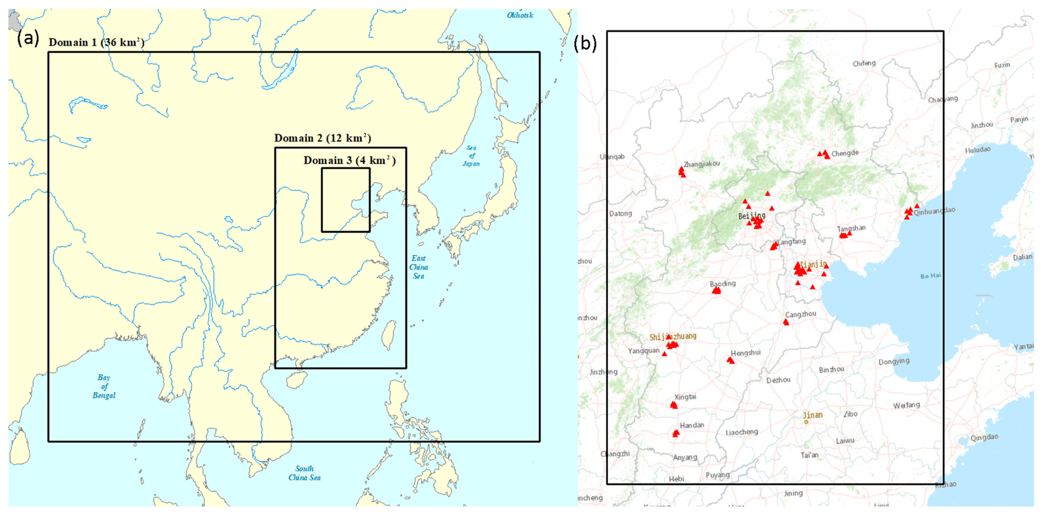
Figure 1The three-domain nested CMAQ domains (a) and the observational sites in the BTH region (b).
In order to minimize the influence of the initial conditions, we choose a 5-day spin-up period. The Carbon Bond 05 (CB05) and AERO6 (Sarwar et al., 2011) are chosen as the gas-phase and aerosol chemical mechanisms, respectively. The simulation periods are January and July of 2014, representing winter and summer, respectively.
We use the Weather Research and Forecasting (WRF) model version 3.7.1 (Skamarock et al., 2008) to simulate the meteorological fields. The physics options for the WRF simulation are the Kain–Fritsch cumulus scheme (Kain, 2004), the Morrison double-moment scheme for cloud microphysics (Morrison et al., 2005), the Pleim–Xiu land surface model (Xiu and Pleim, 2001), the Pleim–Xiu surface layer scheme (Pleim, 2006), the Asymmetric Convective Model (ACM2; Pleim) boundary layer parameterization (Pleim, 2007), and the Rapid Radiative Transfer Model for GCMs radiation scheme (Mlawer et al., 1997). The meteorological initial and boundary conditions are generated from the Final Operational Global Analysis data (ds083.2) of the National Center for Environmental Prediction (NCEP) at and 6 h resolutions. Default profile data are used for chemical initial and boundary conditions. The Meteorology Chemistry Interface Processor (MCIP) version 4.1 is applied to process the meteorological data into the format required by CMAQ. The simulated wind speed, wind direction, temperature, and humidity agree well with the observation data from the National Climate Data Center (NCDC), as detailed in the Supplement.
In order to evaluate the high-resolution emission inventory with the unit-based industrial sources, we develop a traditional proxy-based emission inventory with the same amount of emissions and compare the simulation results of these two emission inventories. In the proxy-based emission inventory, all sectors are allocated as area sources using spatial proxies such as population, GDP, road map, and land use data. The proxies used for each sector are described in detail in Table S2. In order to separate the influences of the horizontal and vertical distributions of the emissions, we developed another unit-based inventory with emission heights the same as the proxy-based inventory; we call this inventory the “hypo-unit-based inventory”. The anthropogenic emission inventories for other provinces in China were developed in our previous studies (Wang et al., 2014; Zhao et al., 2018). The emissions outside China are obtained from the MIX emission inventory (Li et al., 2017) for 2010, which is the most current year available. In the simulation with the unit-based inventory, plume rise is calculated using the built-in algorithm in CMAQ. Meteorological data are used to calculate plume rise for all point sources. Then, the plume is distributed into the vertical layers that the plume intersects based on the pressure in each layer.
3.1 Air pollutant emissions in the BTH region
In the BTH region, the emissions of sulfur dioxide (SO2), nitrogen oxide (NOx), PM10, PM2.5, black carbon (BC), organic carbon (OC), non-methane volatile organic compounds (NMVOCs) and ammonia (NH3) were 1417, 2100, 1479, 1106, 213, 289, 2381, and 712 kt in 2014, respectively. Figure 2 shows the sectoral emissions for major pollutants in the BTH region by city. Figure S2 shows the NMVOCs speciation by sector. The emission estimates are compared with previous studies in Fig. S3. Figure 3 shows the locations and emissions of power and industrial sources.
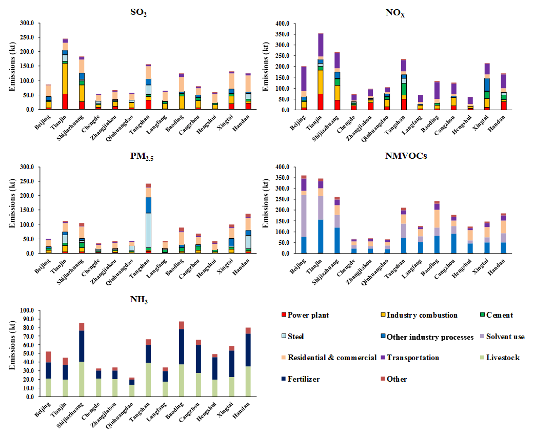
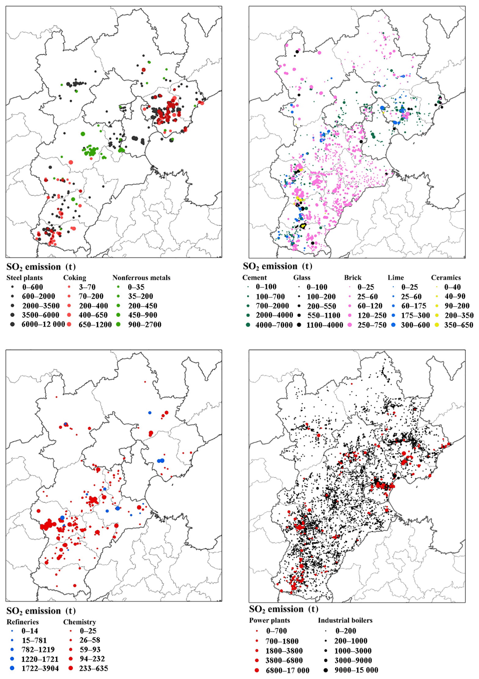
Figure 3Locations and emissions of industrial sources in the BTH region. The industrial plants are divided into four groups for the sake of clarity.
Power plants account for 13 %, 16 %, and 4 % of the total SO2, NOx, and PM2.5 emissions, respectively, whereas the contributions to NMVOC and NH3 emissions are negligible (<1 %). With respect to SO2 and NOx, power plants are important emission sources in the BTH region, especially in Tianjin, Shijiazhuang, Tangshan, and Handan.
The emissions from industrial boilers account for 27 %, 19 %, 8 %, 1 %, and <1 % of the total SO2, NOx, PM2.5, NMVOCs, and NH3 emissions, respectively. As shown in Fig. 3, there are many industrial boilers in the BTH region. Industrial boilers are one of the most important emission sources for SO2 and NOx.
The emissions from cement contribute 6 %, 9 %, and 10 % of the total SO2, NOx, and PM2.5 emissions, respectively, whereas the contributions to NMVOC and NH3 emissions are negligible (<1 %). Most cement plants are located in southern and eastern Hebei.
The emissions from steel production represent 8 %, 3 %, and 22 % of the total SO2, NOx, and PM2.5 emissions, respectively, whereas the contributions to NMVOC and NH3 emissions are negligible (<1 %). Tangshan has the largest number of steel plants in the BTH region, and steel production accounts for over half of the PM2.5 emissions in Tangshan.
Besides the aforementioned sectors, 8 %, 8 %, 13 %, 36 %, and <1 % of the total respective SO2, NOx, PM2.5, NMVOCs, and NH3 emissions come from other industrial processes (chemistry, coking plants, nonferrous metal smelting, brick, ceramics, lime, glass, and refineries). Industrial processes are the most important emission source for NMVOCs, accounting for nearly half of the emissions in Tianjin and Shijiazhuang.
In total, in the BTH region, industrial sectors (power plants, industrial boilers, cement, steel plants, and other industrial processes) contributed 61 %, 55 %, 62 %, 56 %, 58 %, 22 %, 36 %, and 0 % of the total respective SO2, NOx, PM10, PM2.5, BC, OC, NMVOCs, and NH3 emissions in 2014.
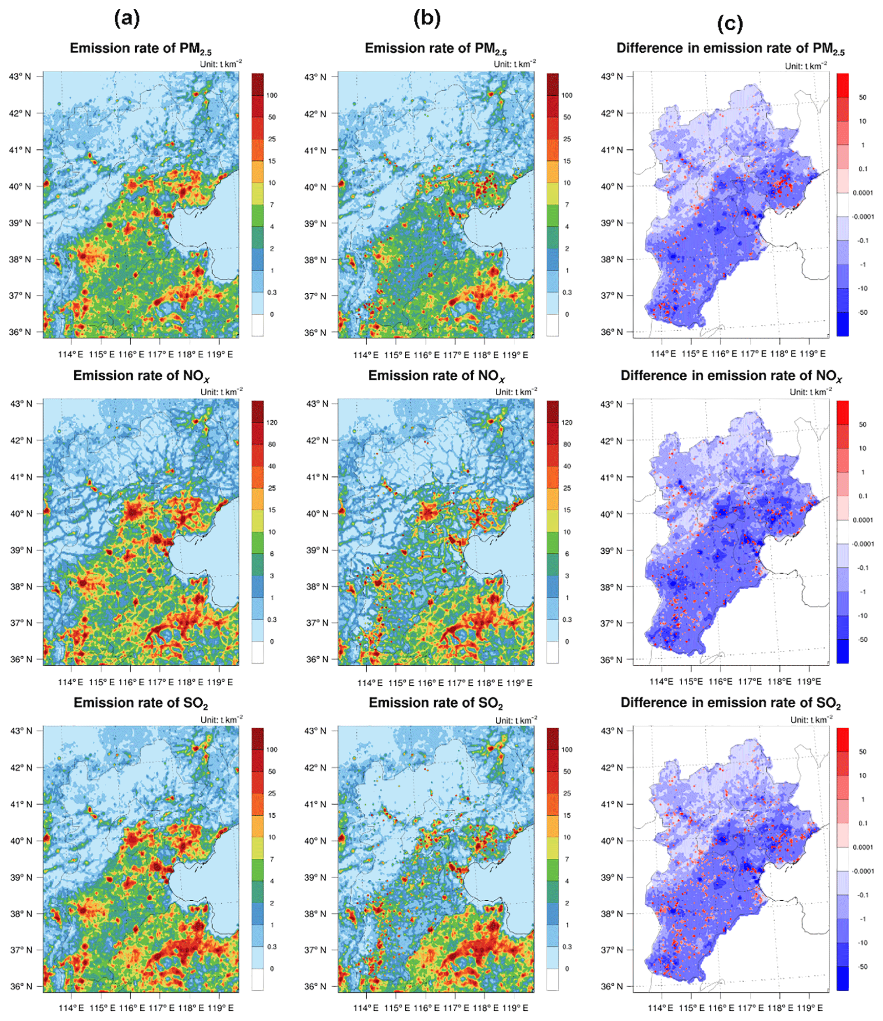
Figure 4Emission rate of PM2.5, NOx, and SO2 emissions of the proxy-based (a) and the unit-based (b) inventories and their differences (unit-based minus proxy-based)( c). Note that the emissions are the same in provinces other than Beijing, Tianjin, and Hebei.
Considering the large contribution of industrial sources to the total emissions, the application of a unit-based method results in remarkable changes in the spatial distribution of air pollutant emissions. The emission rates of PM2.5, NOx, and SO2 in the proxy-based and the unit-based inventories and their differences are shown in Fig. 4. In the unit-based emission inventory, the emissions are lower than those in the proxy-based emission inventory in urban centers in the BTH region. Instead, a large amount of the emissions are concentrated in certain points in suburban areas, where large plants are located.
3.2 Evaluation of the unit-based emission inventory
In order to study the accuracy of the unit-based inventory, the simulation results of SO2, NO2, O3, and PM2.5 with the unit-based inventory are compared with the observational data from the China National Environmental Monitoring Centre. The observations are available for 80 sites located in 13 cities in the BTH region, including 70 sites in urban areas and 10 sites in suburban areas. The accurate locations of urban and suburban sites in Beijing are shown in Figs. S5–S6. The analysis of the results is shown in Table 1. We use the normalized mean bias (NMB), the normalized mean error (NME), the mean fractional bias (MFB), and the mean fractional error (MFE) (U.S. EPA, 2007) to quantitatively evaluate the model performance.
Table 1The statistics for model performance of PM2.5, NO2, SO2, 1 h-peak O3 and daily maximum 8 h averaged (MDA8) O3 in January and July of 2014 with the proxy-based and the unit-based inventories. The following abbreviations are used in the table: simulated (SIM), observed (OBS), normalized mean bias (NMB), normalized mean error (NME), mean fractional bias (MFB), and mean fractional error (MFE).
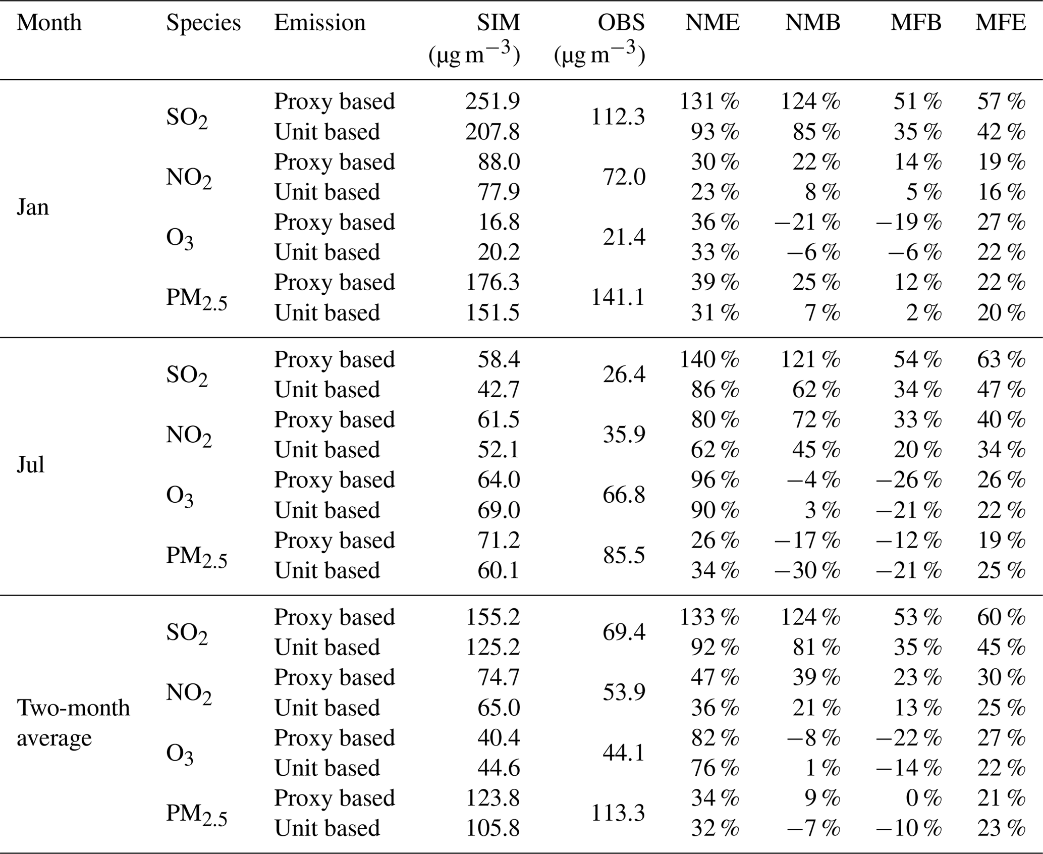
SO2 and NO2 are precursors of PM2.5, so we first compare the simulation results of gaseous pollutants with observations. For NO2, the results with the proxy-based inventory overestimate the observations by 22 %, whereas results with the unit-based inventory overestimate the observations by 9 % in January. Similarly, in July, the simulated NO2 concentrations show an overestimation in simulations with both inventories, but the overestimation is less with the unit-based inventory. The simulation results of SO2 are similar to those of NO2. However, the overestimation is higher with both inventories, and the differences between the concentrations with the two inventories are larger. The overestimation of SO2 concentrations may be due to the lack of several SO2 reaction mechanisms in CMAQ, such as heterogeneous reactions of SO2 on the surface of dust particles (Fu et al., 2016), the oxidation of SO2 by NOx in aerosol liquid water (Cheng et al., 2016; G. Wang et al., 2016), and the effects of SO2 and NH3 on secondary organic aerosol formation (Chu et al., 2016). It may also be due to uncertainty in the emission inventory, especially the uncertainty regarding the removal efficiencies of SO2 control facilities. The biased spatial distribution of SO2 emissions from residential combustion may also contribute to the overestimation. A large fraction of residential combustion takes place in rural areas. However, in this work the emissions from residential combustion are allocated by GDP and population, which leads to an overestimation of SO2 emissions in urban areas and hence an overestimation of the SO2 concentration.
Table 2The statistics for model performance of 1 h-peak NO2 and daily maximum 8 h averaged (MDA8) O3 concentrations in July of 2014 with the proxy-based and the unit-based inventories. See the caption of Table 1 for an explanation of the abbreviations used.
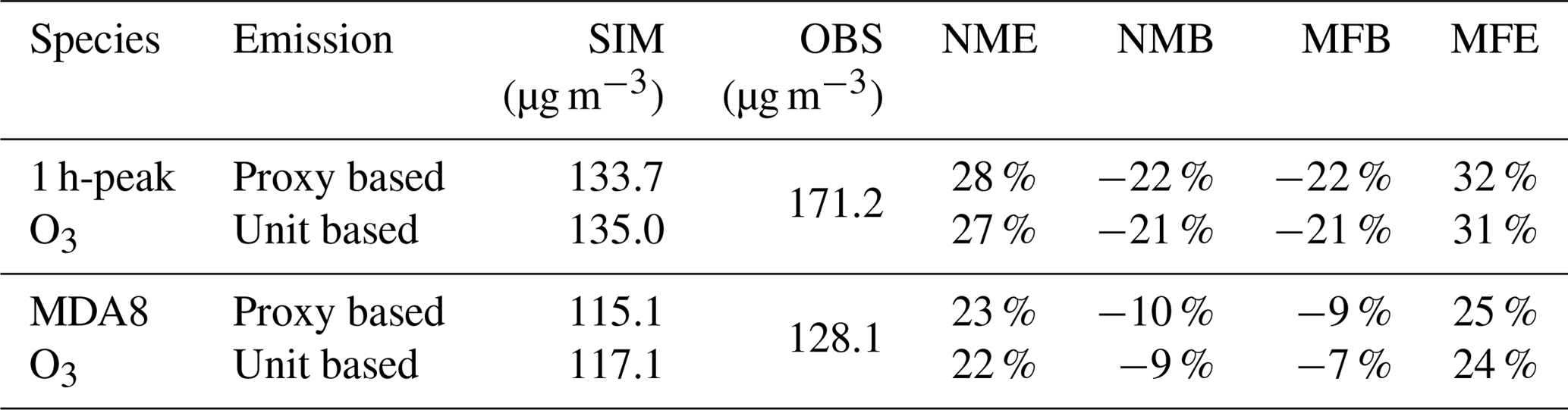
For O3, the simulation results in January with the proxy-based inventory underestimate the observations by 21 %, whereas the results with the unit-based inventory underestimate the observations by only 5 %. The simulation results in July follow the same trend. China is experiencing increasingly severe O3 pollution (Li et al., 2019), which usually occurs in summer. Therefore, we analyze two extra indices of O3, 1 h-peak O3 and daily maximum 8 h averaged (MDA8) O3 concentrations in July, which are shown in Table 2. The results of 1 h-peak O3 and MDA8 O3 concentrations are similar to those of the monthly average O3 concentration. The concentration with the unit-based inventory is slightly higher than that with the proxy-based inventory and is also closer to the observation. The reason for the changes in the O3 concentrations will be discussed later.
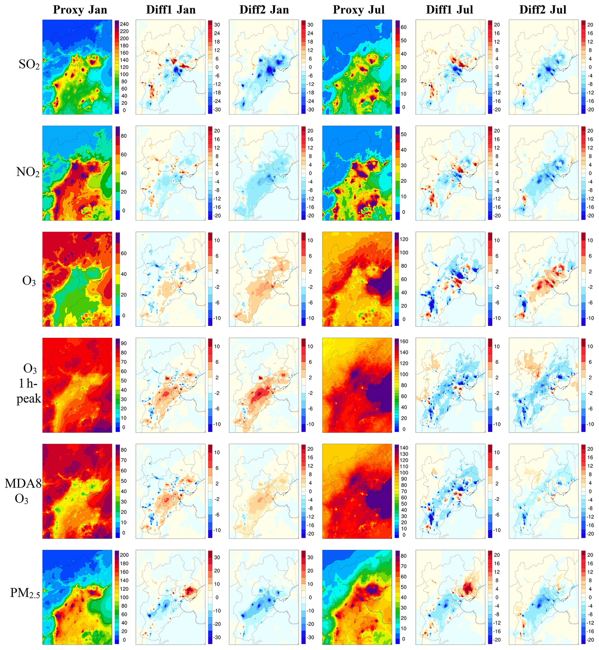
Figure 5Spatial distribution of the monthly (January and July) mean concentrations of SO2, NO2, O3, 1 h-peak O3, MDA8 O3, and PM2.5 with the proxy-based inventory, and the differences between the other two simulations and the proxy-based inventory (Diff1 refers to the hypo-unit-based minus proxy-based, and Diff2 denotes the unit-based minus the proxy-based). The units are µg m−3 for all panels.
The simulated PM2.5 concentrations with the unit-based inventory are lower than those with the proxy-based inventory in both winter and summer. In January, the simulated PM2.5 concentrations with the proxy-based inventory overestimate the observed values by 25 %, whereas the overestimation is only 7 % with the unit-based inventory. In July, the simulated PM2.5 concentrations with both inventories are 17 % and 30 % lower than the observations, respectively. An overall underestimation is expected because the default CMAQ model significantly underestimates the concentrations of secondary organic aerosols (Zhao et al., 2016) and the fugitive dust emission is not included in the emission inventory. According to Boylan and Russell (2006), the simulation results of PM are acceptable when the mean fractional bias (MFB) is less than or equal to ±60 % and the mean fractional error (MFE) is less than 75 %; furthermore, a model performance goal is met when the MFB is less than ±30 % and the MFE is less than 50 %. The statistical indices of the simulation results for PM2.5 with both inventories and both months are within the performance goal values, which means that the simulation results are relatively accurate.
Figure 5 further shows the spatial distribution of SO2, NO2, O3, 1 h-peak O3, MDA8 O3, and PM2.5 concentrations with the proxy-based inventory, and the differences between the other two simulations and the proxy-based inventory. For SO2, NO2, and PM2.5, the concentrations in urban areas are generally higher with the proxy-based inventory than those with the unit-based inventory, especially in winter. In January, large differences with respect to simulated concentrations with the two inventories are found in urban Tianjin, Tangshan, Baoding, and Shijiazhuang, where a large amount of industrial emissions are allocated in the proxy-based inventory due to the large population densities in these areas. The simulations for July follow the same pattern but the concentrations and the differences between the concentrations with the two inventories are lower than those for January. In some areas where many factories are located, such as the northern part of Xingtai city, the concentration with the unit-based inventory is higher because of the high emission intensity. There are two reasons for the difference between the results with the two inventories. The first reason is the spatial distribution. With detailed information regarding the industrial sectors, more emissions are allocated to certain locations in suburban/rural areas in the unit-based emission inventory. From “Diff1” (hypo-unit-based minus proxy-based), we can see that the improved horizontal distribution of the unit-based emission inventory significantly decreases the PM2.5, SO2, and NO2 concentrations in most urban centers, and significantly increases the concentrations in a large fraction of suburban and rural areas, especially the areas where large industrial plants are located. The other reason is the vertical distribution. Plume rise is calculated in the simulation with the unit-based inventory, which causes the difference in emissions in the vertical layers. Therefore, the higher the pollutants are emitted, the lower the ground concentration becomes. From the differences between Diff1 and Diff2 we can see that plume rise leads to lower concentrations over the whole region.
For O3, the difference in the concentrations is evident but is opposite to that for PM2.5. This is because the urban centers of Beijing/Tianjin are located within the VOC-control chemical regime (Liu et al., 2010). Hence, the emissions of NOx in the surface layer are lower in the unit-based inventory than in the proxy-based inventory, which leads to higher O3 concentrations in urban areas.
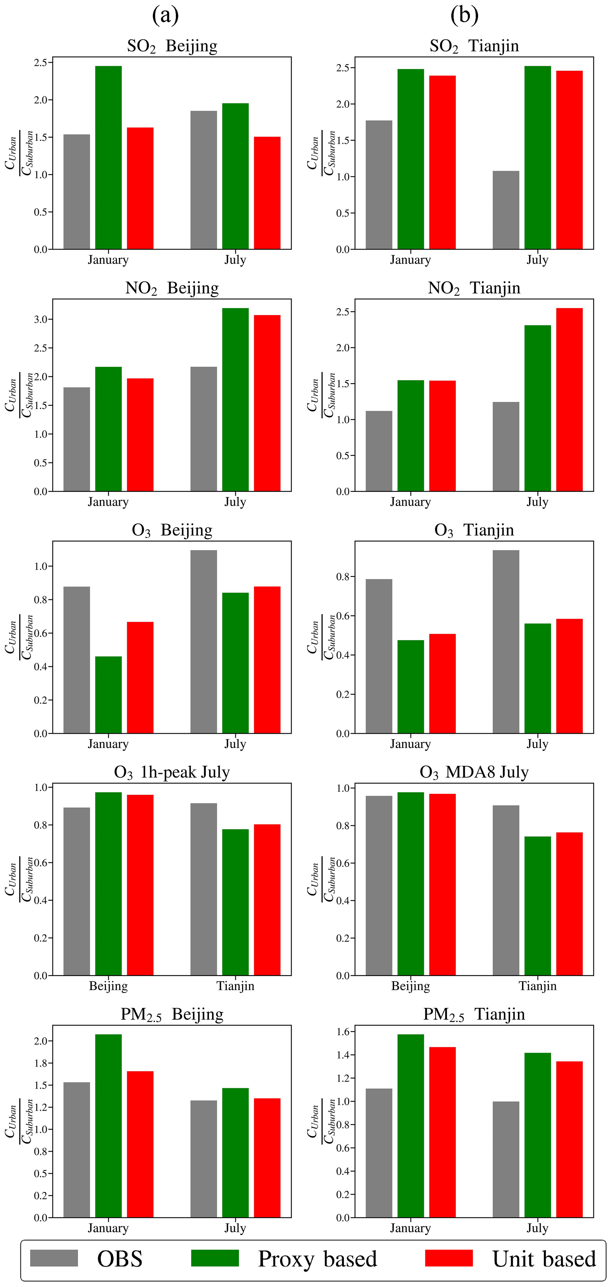
Figure 6Observed and simulated concentration gradients of SO2, NO2, O3, and PM2.5 with the proxy-based and the unit-based inventories in Beijing (a) and Tianjin (b).
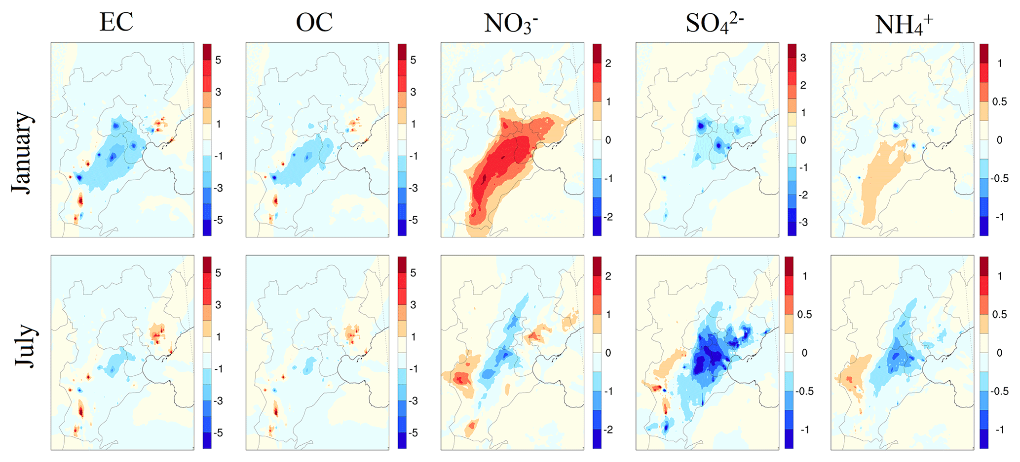
Figure 7The differences (unit: µg m−3) in the simulation results of the components of PM2.5 between the results from the two inventories (unit-based minus proxy-based).
The spatial distribution of the concentrations of these pollutants are significantly heterogeneous. The NME and MFE of most pollutants averaged over a 2-month period are lower with the unit-based inventory than with the proxy-based inventory; this means that the spatial distribution with the unit-based inventory agrees more with the observations than that of the proxy-based inventory. For SO2, NO2, and PM2.5, peak concentrations usually occur in the urban center whereas the opposite is noted for O3. We apply the “concentration gradient” metric, which is defined as the ratio of the urban monthly mean concentrations to the suburban concentrations, to quantitatively characterize the heterogeneous spatial distributions. We calculate the concentration gradients for Beijing and Tianjin (Fig. 6), as both urban and suburban observational sites are found in these two cities. The concentration gradients of NO2 and SO2 between the urban and suburban areas are closer to the observations in the simulation with the unit-based inventory than those with the proxy-based inventory (Fig. 6). The simulated O3 concentration gradients with the unit-based inventory, the proxy-based inventory, and the observations are 0.7, 0.5, and 0.9 in January and 0.9, 0.8, and 1.1 in July, respectively. As for the 1h-peak O3 and MDA8 O3 in July, the simulated results with the unit-based inventory are also closer to the observations. As previously stated, this is explained by the VOC-limited photochemical regime and lower NOx emissions in the unit-based inventory over urban areas. As for PM2.5, the concentration gradients for simulations with the unit-based inventory, the proxy-based inventory, and the observations in Beijing are 1.6, 2.1, and 1.5 in January and 1.3, 1.5, and 1.3 in July, respectively. The results imply that the unit-based emission inventory better reproduces the distributions of pollutant emissions between the urban and suburban areas.
Table 3The mean concentrations (unit: µg m−3) of the components of PM2.5 with the proxy-based and the unit-based inventories and their differences. The following species are listed in this table: sulfate (), nitrate (), ammonium (), elemental carbon (EC), and organic carbon (OC).

To further elucidate the reasons for the difference between the PM2.5 concentrations with two emission inventories, we examine the simulation results of different chemical components, including sulfate (), nitrate (), ammonium (), elemental carbon (EC), and organic carbon (OC), as shown in Fig. 7 and Table 2. The concentrations of EC and OC in the simulation with the unit-based inventory are generally lower than those with the proxy-based inventory in both January and July, especially in urban Beijing, Baoding, and Shijiazhuang. This pattern is similar to that of PM2.5. In some cities such as Xingtai, the concentrations of EC and OC in the simulation with the unit-based inventory are slightly higher than those with the proxy-based inventory.
The results for secondary inorganic aerosols are quite different. From Fig. 7 and Table 3 we can see that the concentrations are lower in most areas in the simulation with the unit-based inventory compared with concentrations with the proxy-based inventory, which is due to the fact that the sensitivity of concentrations to SO2 concentrations is positive during all months (B. Zhao et al., 2017). The differences in the concentrations of are similar to those of SO2, which is shown in Fig. 5. The difference in the concentration is relatively small compared with other components. As for , the concentration of in the simulation with the unit-based inventory is much higher than that with the proxy-based inventory in winter, whereas the differences between the results with two inventories vary with location in summer. concentrations in the unit-based approach are much lower than in the proxy-based approach, whereas is almost constant, as shown in Fig. 7. In this case, more HNO3 is converted to with excess , whereas these processes depend on abundance of HNO3 or NH3. Taking all of the chemical components into account, the primary components account for most of the differences in the PM2.5 concentrations between the simulations with the two inventories. However, the complex responses of various secondary components often counteract each other (especially in January), leading to an overall smaller contribution of secondary components to the PM2.5 concentration differences.
In this study, we developed a high-resolution emission inventory of major pollutants for the BTH region for the year 2014 using unit-based emissions from industrial sectors. The emissions of SO2, NOx, PM10, PM2.5, BC, OC, and NMVOCs from industrial sectors were 869, 1164, 910, 622, 71, 63, and 1390 kt respectively, accounting for a respective 61 %, 55 %, 62 %, 56 %, 58 %, 22 %m and 36 % of the total emissions.
The emissions in the unit-based emission inventory are lower than those in the proxy-based emission inventory in most urban centers in the BTH region due to the concentrated emissions from point sources. The application of the unit-based emission inventory improves model–observation agreement for most pollutants. The accurate location of point sources leads to lower concentrations of primary pollutants in urban areas and higher concentrations in suburban areas. Plume rise accounts for the lower concentrations over the whole region. For SO2, NO2, and PM2.5, the concentrations in urban areas decrease significantly and become closer to the observations, mostly due to the decrease in urban emissions. For O3, the concentrations in urban areas increase slightly and also show better agreement with observations, mainly due to the more reasonable allocation of NOx emissions. The improvement is particularly significant for the urban–suburban concentration gradients. For PM2.5, the concentration gradients for the simulations with the unit-based inventory, the proxy-based inventory, and the observations in Beijing are 1.6, 2.1, and 1.5 in January and 1.3, 1.5, and 1.3 in July, respectively. For O3, the corresponding values are 0.7, 0.5, and 0.9 in January and 0.9, 0.8, and 1.1 in July, implying that the unit-based emission inventory better reproduces the distributions of pollutant emissions between the urban and suburban areas.
The unit-based industrial emission inventory enables more accurate source apportionment and more reliable research on the mechanism of air pollution formation; therefore, it contributes to the development of more precisely targeted control policies. To further improve the emission inventory, it is necessary to improve the spatial allocation of emissions from non-industrial sectors, such as the residential and commercial sectors. Our previous study provides an example of the development of a village-based residential emission inventory in rural Beijing (Cai et al., 2018). Such studies on high-resolution emission inventories, for both industrial and non-industrial sources, are highly needed and should also be extended to other provinces and/or regions. In addition, the plume-in-grid approach might help to further improve model performance, which merits further in-depth study.
All data needed to evaluate the conclusion of this paper are provided in the main text and the Supplement. Additional related data are available upon request.
The supplement related to this article is available online at: https://doi.org/10.5194/acp-19-3447-2019-supplement.
SW and BZ designed the research. HZ, SC, and XC performed the research. HZ, SC, BZ, SW, and XC analyzed the results. HZ, SC, BZ, SW, XC, and JH wrote the paper. HZ and SC contributed equally to this study.
The authors declare that they have no conflict of interest.
This article is part of the special issue “Regional assessment of air pollution and climate change over East and Southeast Asia: results from MICS-Asia Phase III”. It is not associated with a conference.
This research has been supported by the National Key Research and Development Program of the Ministry of Science and Technology of China (grant no. 2017YFC0213005), the National Natural Science Foundation of China (grant no. 21625701), the Strategic Priority Research Program of Chinese Academy of Sciences (grant no. XDA20040502), the National Research Program for Key Issues in Air Pollution Control (grant no. DQGG0301), and the Beijing Municipal Commission of Science and Technology (grant no. D171100001517001). The simulations were completed on the “Explorer 100” cluster system of Tsinghua National Laboratory for Information Science and Technology.
This paper was edited by Yafang Cheng and reviewed by two anonymous referees.
Beijing Municipal Bureau of Statistics: Beijing Statistical Yearbook 2014, China Statistics Press, Beijing, China, 2015.
Boylan, J. W. and Russell, A. G.: PM and light extinction model performance metrics, goals, and criteria for three-dimensional air quality models, Atmos. Environ., 40, 4946–4959, https://doi.org/10.1016/j.atmosenv.2005.09.087, 2006.
Briggs, G. A.: Plume Rise Predictions, in: Lectures on Air Pollution and Environmental Impact Analyses, edited by: Haugen, D. A., American Meteorological Society, Boston, MA, USA, 59–111, 1982.
Cai, S., Li, Q., Wang, S., Chen, J., Ding, D., Zhao, B., Yang, D., and Hao, J.: Pollutant emissions from residential combustion and reduction strategies estimated via a village-based emission inventory in Beijing, Environ. Pollut., 238, 230–237, https://doi.org/10.1016/j.envpol.2018.03.036, 2018.
Chen, L., Sun, Y., Wu, X., Zhang, Y., Zheng, C., Gao, X., and Cen, K.: Unit-based emission inventory and uncertainty assessment of coal-fired power plants, Atmos. Environ., 99, 527–535, https://doi.org/10.1016/j.atmosenv.2014.10.023, 2014.
Chen, W., Hong, J., and Xu, C.: Pollutants generated by cement production in China, their impacts, and the potential for environmental improvement, J. Clean. Prod., 103, 61–69, https://doi.org/10.1016/j.jclepro.2014.04.048, 2015.
Cheng, Y., Zheng, G., Wei, C., Mu, Q., Zheng, B., Wang, Z., Gao, M., Zhang, Q., He, K., Carmichael, G., Poschl, U., and Su, H.: Reactive nitrogen chemistry in aerosol water as a source of sulfate during haze events in China, Sci. Adv., 2, e1601530, https://doi.org/10.1126/sciadv.1601530, 2016.
China Electricity Council: Annual Development Report for China Electric Power Industry 2014, China Statistics Press, Beijing, China, 2015a.
China Electricity Council: Compilation of power industry statistics 2014, China Electricity Council, Beijing, China, 2015b.
China National Environmental Monitoring Centre: Platform for Real-time Urban Air Quality Data, http://106.37.208.233:20035/ (last access: 11 March 2019), 2018.
Chinese State Council: Atmospheric Pollution Prevention and Control Action Plan, Chinese State Council, Beijing, China, 2013.
Chu, B., Zhang, X., Liu, Y., He, H., Sun, Y., Jiang, J., Li, J., and Hao, J.: Synergetic formation of secondary inorganic and organic aerosol: effect of SO2 and NH3 on particle formation and growth, Atmos. Chem. Phys., 16, 14219–14230, https://doi.org/10.5194/acp-16-14219-2016, 2016.
U.S. Environmental Protection Agency (U.S. EPA): Guidance on the Use of Models and Other Analyses for Demonstrating Attainment of Air Quality Goals for Ozone, PM2.5, and Regional Haze, North Carolina, USA, 2007.
Fu, X., Wang, S. X., Zhao, B., Xing, J., Cheng, Z., Liu, H., and Hao, J. M.: Emission inventory of primary pollutants and chemical speciation in 2010 for the Yangtze River Delta region, China, Atmos. Environ., 70, 39–50, https://doi.org/10.1016/j.atmosenv.2012.12.034, 2013.
Fu, X., Wang, S., Chang, X., Cai, S., Xing, J., and Hao, J.: Modeling analysis of secondary inorganic aerosols over China: pollution characteristics, and meteorological and dust impacts, Sci. Rep., 6, 35992, https://doi.org/10.1038/srep35992, 2016.
Geng, G., Zhang, Q., Martin, R. V., Lin, J., Huo, H., Zheng, B., Wang, S., and He, K.: Impact of spatial proxies on the representation of bottom-up emission inventories: A satellite-based analysis, Atmos. Chem. Phys., 17, 4131–4145, https://doi.org/10.5194/acp-17-4131-2017, 2017.
Hebei Municipal Bureau of Statistics: Hebei Statistical Yearbook 2014, China Statistics Press, Hebei, China, 2015.
Kain, J. S.: The Kain-Fritsch convective parameterization: An update, J. Appl. Meteorol., 43, 170–181, https://doi.org/10.1175/1520-0450(2004)043<0170:tkcpau>2.0.co;2, 2004.
Lei, Y., Zhang, Q., Nielsen, C., and He, K.: An inventory of primary air pollutants and CO2 emissions from cement production in China, 1990–2020, Atmos. Environ., 45, 147–154, https://doi.org/10.1016/j.atmosenv.2010.09.034, 2011.
Li, K., Jacob, D. J., Liao, H., Shen, L., Zhang, Q., and Bates, K. H.: Anthropogenic drivers of 2013–2017 trends in summer surface ozone in China, P. Natl. Acad. Sci. USA, 116, 422–427, https://doi.org/10.1073/pnas.1812168116, 2019.
Li, M., Zhang, Q., Kurokawa, J.-I., Woo, J.-H., He, K., Lu, Z., Ohara, T., Song, Y., Streets, D. G., Carmichael, G. R., Cheng, Y., Hong, C., Huo, H., Jiang, X., Kang, S., Liu, F., Su, H., and Zheng, B.: MIX: a mosaic Asian anthropogenic emission inventory under the international collaboration framework of the MICS-Asia and HTAP, Atmos. Chem. Phys., 17, 935–963, https://doi.org/10.5194/acp-17-935-2017, 2017.
Liu, F., Zhang, Q., Tong, D., Zheng, B., Li, M., Huo, H., and He, K. B.: High-resolution inventory of technologies, activities, and emissions of coal-fired power plants in China from 1990 to 2010, Atmos. Chem. Phys., 15, 13299–13317, https://doi.org/10.5194/acp-15-13299-2015, 2015.
Liu, X. H., Zhang, Y., Xing, J., Zhang, Q. A., Wang, K., Streets, D. G., Jang, C., Wang, W. X., and Hao, J. M.: Understanding of regional air pollution over China using CMAQ, part II. Process analysis and sensitivity of ozone and particulate matter to precursor emissions, Atmos. Environ., 44, 3719–3727, https://doi.org/10.1016/j.atmosenv.2010.03.036, 2010.
Ministry of Environmental Protection of China: Emission standard of air pollutants for industrial kiln and furnace, Ministry of Environmental Protection of China (MEP), Beijing, China, 1997.
Ministry of Environmental Protection of China: Emission standard of air pollutants for cement industry, Ministry of Environmental Protection of China (MEP), Beijing, China, 2013.
Mlawer, E. J., Taubman, S. J., Brown, P. D., Iacono, M. J., and Clough, S. A.: Radiative transfer for inhomogeneous atmospheres: RRTM, a validated correlated-k model for the longwave, J. Geophys. Res.-Atmos., 102, 16663–16682, https://doi.org/10.1029/97jd00237, 1997.
Morrison, H., Curry, J. A., and Khvorostyanov, V. I.: A new double-moment microphysics parameterization for application in cloud and climate models. Part I: Description, J. Atmos. Sci., 62, 1665–1677, https://doi.org/10.1175/jas3446.1, 2005.
National Bureau of Statistics (NBS): Report of the first national census of pollution sources, China Statistics Press, Beijing, China, 2010.
National Bureau of Statistics (NBS): China Steel Yearbook 2011, China Statistics Press, Beijing, China, 2012.
National Bureau of Statistics (NBS): China Regional Economic Statistical Yearbook 2014, China Statistics Press, Beijing, China, 2015a.
National Bureau of Statistics (NBS): China Rural Statistical Yearbook 2014, China Statistics Press, Beijing, China, 2015b.
National Bureau of Statistics (NBS): China Statistical Yearbook 2014, China Statistics Press, Beijing, China, 2015c.
National Bureau of Statistics (NBS): China Urban Construction Statistical Yearbook 2014, China Statistics Press, Beijing, China, 2015d.
National Bureau of Statistics (NBS): China Energy Statistical Yearbook 2014, China Statistics Press, Beijing, China, 2015e.
National Bureau of Statistics (NBS): China Electric Power Yearbook 2014, China Statistics Press, Beijing, China, 2015f.
National Bureau of Statistics (NBS): China Chemical Industry yearbook 2014, China Statistics Press, Beijing, China, 2015g.
National Bureau of Statistics (NBS): China Agriculture Yearbook 2014, China Statistics Press, Beijing, China, 2015h.
National Bureau of Statistics (NBS): China Environmental Statistical Yearbook 2014, China Statistics Press, Beijing, China, 2015i.
National Bureau of Statistics (NBS): China Industrial Economic Statistical Yearbook 2014, China Statistics Press, Beijing, China, 2015j.
Oda, T. and Maksyutov, S.: A very high-resolution (1 km × 1 km) global fossil fuel CO2 emission inventory derived using a point source database and satellite observations of nighttime lights, Atmos. Chem. Phys., 11, 543–556, https://doi.org/10.5194/acp-11-543-2011, 2011.
Ohara, T., Akimoto, H., Kurokawa, J., Horii, N., Yamaji, K., Yan, X., and Hayasaka, T.: An Asian emission inventory of anthropogenic emission sources for the period 1980–2020, Atmos. Chem. Phys., 7, 4419–4444, https://doi.org/10.5194/acp-7-4419-2007, 2007.
Pleim, J. E.: A simple, efficient solution of flux-profile relationships in the atmospheric surface layer, J. Appl. Meteorol. Clim., 45, 341–347, https://doi.org/10.1175/jam2339.1, 2006.
Pleim, J. E.: A Combined Local and Nonlocal Closure Model for the Atmospheric Boundary Layer. Part II: Application and Evaluation in a Mesoscale Meteorological Model, J. Appl. Meteorol. Clim., 46, 1396–1409, https://doi.org/10.1175/jam2534.1, 2007.
Qi, J., Zheng, B., Li, M., Yu, F., Chen, C., Liu, F., Zhou, X., Yuan, J., Zhang, Q., and He, K.: A high-resolution air pollutants emission inventory in 2013 for the Beijing–Tianjin–Hebei region, China, Atmos. Environ., 170, 156–168, https://doi.org/10.1016/j.atmosenv.2017.09.039, 2017.
Sarwar, G., Appel, K. W., Carlton, A. G., Mathur, R., Schere, K., Zhang, R., and Majeed, M. A.: Impact of a new condensed toluene mechanism on air quality model predictions in the US, Geosci. Model Dev., 4, 183–193, https://doi.org/10.5194/gmd-4-183-2011, 2011.
Skamarock, W. C., Dudhia, J. B. K. J., Gill, D. O., Barker, D., Wang, W., and Powers, J. G.: A Description of the Advanced Research WRF Version 3, NCAR Technical Note NCAR/TN-475+STR, https://doi.org/10.5065/D68S4MVH, 2008.
Stohl, A., Aamaas, B., Amann, M., Baker, L. H., Bellouin, N., Berntsen, T. K., Boucher, O., Cherian, R., Collins, W., Daskalakis, N., Dusinska, M., Eckhardt, S., Fuglestvedt, J. S., Harju, M., Heyes, C., Hodnebrog, Ø., Hao, J., Im, U., Kanakidou, M., Klimont, Z., Kupiainen, K., Law, K. S., Lund, M. T., Maas, R., MacIntosh, C. R., Myhre, G., Myriokefalitakis, S., Olivié, D., Quaas, J., Quennehen, B., Raut, J.-C., Rumbold, S. T., Samset, B. H., Schulz, M., Seland, Ø., Shine, K. P., Skeie, R. B., Wang, S., Yttri, K. E., and Zhu, T.: Evaluating the climate and air quality impacts of short-lived pollutants, Atmos. Chem. Phys., 15, 10529–10566, https://doi.org/10.5194/acp-15-10529-2015, 2015.
Streets, D. G., Bond, T. C., Carmichael, G. R., Fernandes, S. D., Fu, Q., He, D., Klimont, Z., Nelson, S. M., Tsai, N. Y., Wang, M. Q., Woo, J. H., and Yarber, K. F.: An inventory of gaseous and primary aerosol emissions in Asia in the year 2000, J. Geophys. Res.-Atmos., 108, 8809, https://doi.org/10.1029/2002jd003093, 2003.
Tianjin Municipal Bureau of Statistics: Tianjin Statistical Yearbook 2014, China Statistics Press, Tianjin, China, 2015.
Wang, G., Zhang, R., Gomez, M. E., Yang, L., Levy Zamora, M., Hu, M., Lin, Y., Peng, J., Guo, S., Meng, J., Li, J., Cheng, C., Hu, T., Ren, Y., Wang, Y., Gao, J., Cao, J., An, Z., Zhou, W., Li, G., Wang, J., Tian, P., Marrero-Ortiz, W., Secrest, J., Du, Z., Zheng, J., Shang, D., Zeng, L., Shao, M., Wang, W., Huang, Y., Wang, Y., Zhu, Y., Li, Y., Hu, J., Pan, B., Cai, L., Cheng, Y., Ji, Y., Zhang, F., Rosenfeld, D., Liss, P. S., Duce, R. A., Kolb, C. E., and Molina, M. J.: Persistent sulfate formation from London Fog to Chinese haze, P. Natl. Acad. Sci. USA, 113, 13630–13635, https://doi.org/10.1073/pnas.1616540113, 2016.
Wang, K., Tian, H., Hua, S., Zhu, C., Gao, J., Xue, Y., Hao, J., Wang, Y., and Zhou, J.: A comprehensive emission inventory of multiple air pollutants from iron and steel industry in China: Temporal trends and spatial variation characteristics, Sci. Total Environ., 559, 7–14, https://doi.org/10.1016/j.scitotenv.2016.03.125, 2016.
Wang, S. X., Zhao, B., Cai, S. Y., Klimont, Z., Nielsen, C. P., Morikawa, T., Woo, J. H., Kim, Y., Fu, X., Xu, J. Y., Hao, J. M., and He, K. B.: Emission trends and mitigation options for air pollutants in East Asia, Atmos. Chem. Phys., 14, 6571–6603, https://doi.org/10.5194/acp-14-6571-2014, 2014.
Wu, W., Zhao, B., Wang, S., and Hao, J.: Ozone and secondary organic aerosol formation potential from anthropogenic volatile organic compounds emissions in China, J. Environ. Sci., 53, 224–237, https://doi.org/10.1016/j.jes.2016.03.025, 2017.
Wu, X., Zhao, L., Zhang, Y., Zheng, C., Gao, X., and Cen, K.: Primary Air Pollutant Emissions and Future Prediction of Iron and Steel Industry in China, Aerosol Air Qual. Res., 15, 1422–1432, https://doi.org/10.4209/aaqr.2015.01.0029, 2015.
Xiu, A. J. and Pleim, J. E.: Development of a land surface model. Part I: Application in a mesoscale meteorological model, J. Appl. Meteorol., 40, 192–209, https://doi.org/10.1175/1520-0450(2001)040<0192:doalsm>2.0.co;2, 2001.
Xue, Y., Tian, H., Yan, J., Zhou, Z., Wang, J., Nie, L., Pan, T., Zhou, J., Hua, S., Wang, Y., and Wu, X.: Temporal trends and spatial variation characteristics of primary air pollutants emissions from coal-fired industrial boilers in Beijing, China, Environ. Pollut., 213, 717–726, https://doi.org/10.1016/j.envpol.2016.03.047, 2016.
Zhao, B., Wang, S., Dong, X., Wang, J., Duan, L., Fu, X., Hao, J., and Fu, J.: Environmental effects of the recent emission changes in China: implications for particulate matter pollution and soil acidification, Environ. Res. Lett., 8, 024031, https://doi.org/10.1088/1748-9326/8/2/024031, 2013a.
Zhao, B., Wang, S. X., Wang, J. D., Fu, J. S., Liu, T. H., Xu, J. Y., Fu, X., and Hao, J. M.: Impact of national NOx and SO2 control policies on particulate matter pollution in China, Atmos. Environ., 77, 453–463, https://doi.org/10.1016/j.atmosenv.2013.05.012, 2013b.
Zhao, B., Wang, S., Donahue, N. M., Jathar, S. H., Huang, X., Wu, W., Hao, J., and Robinson, A. L.: Quantifying the effect of organic aerosol aging and intermediate-volatility emissions on regional-scale aerosol pollution in China, Sci. Rep., 6, 28815, https://doi.org/10.1038/srep28815, 2016.
Zhao, B., Wu, W., Wang, S., Xing, J., Chang, X., Liou, K.-N., Jiang, J. H., Gu, Y., Jang, C., Fu, J. S., Zhu, Y., Wang, J., Lin, Y., and Hao, J.: A modeling study of the nonlinear response of fine particles to air pollutant emissions in the Beijing–Tianjin–Hebei region, Atmos. Chem. Phys., 17, 12031–12050, https://doi.org/10.5194/acp-17-12031-2017, 2017.
Zhao, B., Zheng, H., Wang, S., Smith, K. R., Lu, X., Aunan, K., Gu, Y., Wang, Y., Ding, D., Xing, J., Fu, X., Yang, X., Liou, K. N., and Hao, J.: Change in household fuels dominates the decrease in PM2.5 exposure and premature mortality in China in 2005–2015, P. Natl. Acad. Sci. USA, 115, 12401–12406, 2018.
Zhao, Y., Wang, S. X., Duan, L., Lei, Y., Cao, P. F., and Hao, J. M.: Primary air pollutant emissions of coal-fired power plants in China: Current status and future prediction, Atmos. Environ., 42, 8442–8452, https://doi.org/10.1016/j.atmosenv.2008.08.021, 2008.
Zhao, Y., Mao, P., Zhou, Y., Yang, Y., Zhang, J., Wang, S., Dong, Y., Xie, F., Yu, Y., and Li, W.: Improved provincial emission inventory and speciation profiles of anthropogenic non-methane volatile organic compounds: a case study for Jiangsu, China, Atmos. Chem. Phys., 17, 7733–7756, https://doi.org/10.5194/acp-17-7733-2017, 2017.
Zheng, B., Zhang, Q., Tong, D., Chen, C., Hong, C., Li, M., Geng, G., Lei, Y., Huo, H., and He, K.: Resolution dependence of uncertainties in gridded emission inventories: a case study in Hebei, China, Atmos. Chem. Phys., 17, 921–933, https://doi.org/10.5194/acp-17-921-2017, 2017.
Zhou, Y. and Gurney, K. R.: Spatial relationships of sector-specific fossil fuel CO2emissions in the United States, Global Biogeochem. Cy., 25, GB3002, https://doi.org/10.1029/2010gb003822, 2011.