Local and remote temperature response of regional SO₂ emissions

Short-lived anthropogenic climate forcers (SLCFs), such as sulfate aerosols, affect both climate and air quality. Despite being short-lived, these forcers do not affect temperatures only locally; regions far away from the emission sources are also affected. Climate metrics are often used in a policy context to compare the climate impact of different anthropogenic forcing agents. These metrics typically relate a forcing change in a certain region with a temperature change in another region and thus often require a separate model to convert emission changes to radiative forcing (RF) changes.

In this study, we used a coupled Earth system model, NorESM (Norwegian Earth System Model), to calculate emission-to-temperature-response metrics for sulfur dioxide (SO₂) emission changes in four different policy-relevant regions: Europe (EU), North America (NA), East Asia (EA) and South Asia (SA). We first increased the SO₂ emissions in each individual region by an amount giving approximately the same global average radiative forcing change (−0.45 Wm⁻²). The global mean temperature change per unit sulfur emission compared to the control experiment was independent of emission region and equal to ∼0.006 K(TgSyr⁻¹)⁻¹. On a regional scale, the Arctic showed the largest temperature response in all experiments. The second largest temperature change occurred in the region of the imposed emission increase, except when South Asian emissions were changed; in this experiment, the temperature response was approximately the same in South Asia and East Asia. We also examined the non-linearity of the temperature response by removing all anthropogenic SO₂ emissions over Europe in one experiment. In this case, the temperature response (both global and regional) was twice that in the corresponding experiment with a European emission increase. This non-linearity in the temperature response is one of many uncertainties associated with the use of simplified climate metrics.

1 Introduction

Anthropogenic emissions of short-lived climate forcers (SLCFs), i.e. chemical components in the atmosphere that interact with radiation, have both an immediate effect on local air quality and regional and global effects on the climate in terms of changes in the temperature and precipitation distribution. Aerosol particles are one of the most important SLCFs due to their abundance and their effects on health and climate. The short atmospheric residence times of SLCFs such as sulfate and carbonaceous aerosols (around days) lead to high atmospheric concentrations in emission regions and a highly variable radiative forcing (RF) pattern. Regional radiative forcing can, nevertheless, exert a large influence on the temperature field away from the forcing region through changes in heat transport or the atmospheric or ocean circulation (Menon et al., 2002; Shindell et al., 2010; Lewinschal et al., 2013; Acosta Navarro et al., 2016; Dong et al., 2016). Here, we investigate the effect of sulfate aerosol precursor emission perturbations in different regions on the global surface temperature distribution using a global climate model.

The local radiative forcing by a unit aerosol emission varies from region to region depending on a number of factors, including emission location, aerosol processing in the atmosphere and removal rates, as well as land surface properties and cloud distribution (e.g. Bellouin et al., 2016). Moreover, a unit radiative forcing in a specific region may have different impacts on the temperature response locally in the forcing region and in remote regions away from the forcing, as well as between different remote regions. In other words, the climate sensitivity in one region can vary depending on the location of the forcing (e.g. Shindell and Faluvegi, 2009).

To facilitate comparisons of the climate effect of different greenhouse gases and emission levels, several climate metrics which connect emission changes to radiative forcing or a specified forcing to a temperature response have been developed (e.g. Aamaas et al., 2013). One appeal of simple climate metrics is that they provide a way to easily evaluate the climate impact of different air quality or climate mitigation policies without having to run a coupled climate model, something which is not always feasible due to the computational costs. Because of the even spatial distribution of long-lived greenhouse gases, these metrics have usually described global average quantities. However, the highly variable spatial distribution of aerosol forcing necessitates the use of metrics that take these spatial inhomogeneities into account (Shine et al., 2005).

Shindell and Faluvegi (2009) developed a metric, the regional temperature potential (RTP), that accounts for spatial inhomogeneities in both (i) the forcing and (ii) the temperature response. With a large set of simulations with one climate model, where they varied the location of forcing from various anthropogenic climate forcers, these authors derived RTP coefficients that link the radiative forcing from a climate forcer in a specific region to regional temperature responses. An evaluation of the method for transient simulations of historical aerosol forcing and response with four different climate models was presented in the work of Shindell (2012).

However, the simplification inherent in the climate metric concept might lead to difficulties related to the generality of these metrics, such as the RTP. Differences between RTP coefficients derived from different climate models can stem from a number of different sources, involving everything from atmospheric processing of aerosols, interaction with radiation, aerosol cloud effects or climate feedbacks, and how these processes are represented in different climate models (Kasoar et al., 2016; Conley et al., 2018).

The main objective of this study is to investigate the global and remote impacts of regional sulfate aerosol precursor emission changes on the surface temperature distribution. This is done by using a coupled atmosphere–ocean model with interactive aerosol representation, the Norwegian Earth System Model (NorESM). The results from the model simulations are used to derive RTP coefficients similar to the work of Shindell and Faluvegi (2009). However, our method for deriving RTP coefficients differs from that of Shindell and Faluvegi (2009) in that we derive our RTP coefficients directly from emission perturbations and focus primarily on the emissions–temperature connection rather than the connection between radiative forcing and temperature, similar to Kasoar et al. (2018). The RTP coefficients derived by Shindell and Faluvegi (2009) describe the regional temperature change in response to regional radiative forcing and essentially describe a regional sensitivity. These forcing-based sensitivities have to be combined with the radiative forcing patterns derived from emission scenarios with a chemical transport model (CTM) or offline calculations for radiative forcing with a general circulation model to provide the emission–temperature connection. Another difference is that we focus on emissions from air-pollution and policy-making-relevant regions rather than the latitudinal bands of Shindell and Faluvegi (2009). Thus, we seek to investigate how much an emission change in one policy-relevant region affects both local climate as well as the climate on a global scale and in remote regions.

The aim is that the RTP coefficients derived with NorESM eventually could be used in integrated assessment analysis (IAA), such as the Greenhouse Gas and Air Pollution Interactions and Synergies (GAINS) model. In the GAINS model the climate impact is estimated using the global warming potential (GWP), which is the global radiative forcing integrated over time normalised by that of CO₂ (Amann et al., 2011). Using the GWP, the global climate impact of SLCFs can be taken into account. Lately, the radiative forcing of long-lived greenhouse gases other than CO₂ has been included in GAINS, which makes it possible to evaluate the changes in emissions of these due to air-pollution abatement. Using RTP coefficients in IAA would mean that not only can near-term climate effects of changed SLCF emissions be evaluated but also how different regions are affected due to specific regional abatement measures. The RTP can be based on different entities as radiative forcing, effective radiative forcing (ERF) or direct emissions, which need very different support calculations, respectively. Using the emissions as base for RTPs will provide a very simple way to estimate the climate impact of changed emissions without having to run a chemical transport model. Using any of the bases for the RTPs avoids running large coupled climate models. However, the validity of this method relies on the accuracy of the assumption that the temperature response to changed emissions is linear and that the interactions between different SLCFs are negligible for the resulting temperature response. To address the question regarding linearity in the response depending on emission perturbation strength we perform simulations with different emission perturbations for the European region.

The layout of this study is as follows. First an introduction to the RTP methodology is presented in the method section. The NorESM model is described together with the experimental design to derive the emission-specific RTP coefficients. In Sect. 3 we first present the results from experiments where sulfate aerosol precursor emissions were increased and the global and regional effect of these emission perturbations. The results of an experiment where European anthropogenic sulfate aerosol precursor emissions were removed are discussed in the context of non-linearities emerging as a consequence of emission magnitudes. Last in the results section is a comparison of the performance of the forcing-based RTP coefficients of Shindell and Faluvegi (2009) and Shindell et al. (2012) for NorESM results. The results section is followed by a discussion and conclusions.

2 Method

2.1 The absolute regional temperature potential

There exists a number of different climate metrics that describe the connection between emissions of atmospheric tracer species and/or their radiative forcing and/or their effect on the global mean temperature. Many have been developed for the purpose of evaluating the impact of increased emissions of long-lived and well-mixed greenhouse gases. Thus, the connection between the location of an emission perturbation and the temperature response has not been a primary concern. However, for SLCFs the location of the emission perturbation and radiative forcing is a primary matter of interest. A climate metric which takes the spatial distribution of these SLCFs and the temperature response into account was developed by Shindell and Faluvegi (2009) and Shindell and Faluvegi (2010). The metric describes the temperature change dT in one area a at time t, in response to forcing F in area a^′:

$$\begin{array}{}\text{(1)}& {\displaystyle }\mathrm{d}{T}_{\mathrm{a}}\left(t\right)=\underset{\mathrm{0}}{\overset{t}{\int }}\left(\sum _{{\mathrm{a}}^{\prime }}{F}_{{\mathrm{a}}^{\prime }}\left(t^{\prime }\right)\cdot {\displaystyle \frac{\mathrm{d}{T}_{\mathrm{a}}/F_{{\mathrm{a}}^{\prime }}}{\mathrm{d}{T}_{\mathrm{a}}/F_{\mathrm{global}}}}\right)\cdot \mathrm{IRF}(t-t^{\prime })\mathrm{d}{t}^{\prime },\end{array}$$

where the numerator in the second term of the sum, d$T_{\mathrm{a}}/F_{{\mathrm{a}}^{\prime }}$, is the regional response coefficient (see Table 3 of Shindell and Faluvegi, 2010), which in this formulation is normalised by the regional temperature response to global average forcing, dT_a∕F_global. The impulse response function, IRF, represents the time-dependent temperature response per unit forcing, i.e. the climate sensitivity. For the equilibrium (or quasi-equilibrium or transient) temperature response to a steady forcing, the IRF can be replaced by the equilibrium or transient climate sensitivity, λ.

Shindell (2012) elaborated the regional temperature change metric of Shindell and Faluvegi (2010) to an absolute regional temperature potential, ARTP, which, in analogue to the absolute global temperature change potential (AGTP), connects an emission perturbation, E, in region r of a climate forcer to an absolute temperature change (Shine et al., 2005) in area a:

$$\begin{array}{ll}{\displaystyle }{\mathrm{ARTP}}_{a,r}\left(t\right)& {\displaystyle }=\underset{\mathrm{0}}{\overset{t}{\int }}\left(\sum _{a^{\prime }}{\displaystyle \frac{F_{a^{\prime }}\left(t^{\prime }\right)}{E_r}}\cdot {\displaystyle \frac{\mathrm{d}{T}_a/F_{a^{\prime }}}{\mathrm{d}{T}_{\mathrm{global}}\left(F_{\mathrm{global}}\right)/F_{\mathrm{global}}}}\right)\\ \text{(2)}& {\displaystyle }& {\displaystyle }\cdot \mathrm{IRF}(t-t^{\prime })\mathrm{d}{t}^{\prime }.\end{array}$$

This formulation uses the global climate sensitivity (dT_global(F_global)∕F_global) to normalise the regional response coefficients in contrast to Eq. (1), which uses the regional sensitivity to global forcing. This, i.e. the second term in the summation of Eq. (2), yields the unitless RTP coefficients presented in Table 1 of Shindell (2012). Shindell (2012) also advocates the use of the latter formulation (Eq. 2) before the former (Eq. 1).

The RTP coefficients provided in the work of Shindell and Faluvegi (2010) and Shindell (2012) were derived for forcing in four latitude bands covering the globe: the Southern Hemisphere extratropics (90–28^∘ S, SHext), tropics (28^∘ S–28^∘ N), Northern Hemisphere mid-latitudes (28–60^∘ N, NHml) and Arctic (60–90^∘ N). These RTP coefficients can be used to estimate the global temperature response to any emission perturbation, as long as the forcing in response to the emission perturbation in each of the latitude bands described above is known. The forcing distribution in response to an emission perturbation can be calculated with a chemical transport model (direct radiative forcing only) or with atmospheric general circulation models.

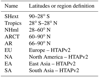
In this work, we take our starting point in emission perturbations rather than in the forcing distribution. Sub-global temperature changes in response to emission perturbations are derived both for latitudinal bands following Shindell and Faluvegi (2009) and for the emission regions defined in this study, with the addition of a complementary Arctic region (AR). This complementary Arctic region is defined as the area north of the Arctic circle (66^∘ N), whereas the northernmost latitudinal band (hereafter denoted ARCT) is defined as the area north of 60^∘ N in accordance with the definition of Shindell and Faluvegi (2009). All regions that are used in this study are listed in Table 1.

Table 1 Latitudinal band definitions and region definitions.

2.2 NorESM

The regional temperature changes in response to aerosol emission perturbations are investigated using NorESM (Bentsen et al., 2013). This model is based on the Community Climate System Model 4.0 (CCSM4.0) but has been modified to include interactive aerosols and to use the Bergen version of the Miami Isopycnic Coordinate Ocean Model (MICOM) instead of the Parallel Ocean Program (POP) model. For NorESM the atmospheric component of the model, the Community Atmospheric Model version 4 (CAM4), has been extended with an interactive aerosol module, CAM4-Oslo (Kirkevåg et al., 2013). The land surface is represented by the Community Land Model version 4 (CLM4) and sea ice is modelled with the ice model CICE4. The atmospheric model uses a finite volume grid with a resolution of $\mathrm{1.9}{}^{\circ }\times \mathrm{2.5}{}^{\circ }$ latitude–longitude.

The aerosol module in NorESM considers five different aerosol components: sulfate, black carbon, organic matter, mineral dust and sea salt. Both the mass and number for these aerosol constituents are predicted in a combined sectional and modal framework. Emissions take place both in the form of primary particles and as precursors to aerosols where the aerosol chemical compounds are produced through aqueous- and gas-phase chemical reactions. Aerosols can exist both as external and internal mixtures, depending on atmospheric processing. For example, sulfate coating of black carbon, which changes the optical and hygroscopic properties of this internally mixed aerosol compared with the externally mixed constituents, is accounted for. Humidification of aerosols is based on the hygroscopicity of the aerosol and the atmospheric relative humidity. Aerosols are removed from the atmosphere by dry and wet deposition.

Aerosol can affect cloud properties through acting as cloud condensation nuclei (CCN). The efficiency of a particular aerosol depends on its hygroscopicity and size. The number of aerosol particles that are efficient CCN is connected to the predicted aerosol size and mass, and it is connected to the two-moment cloud microphysics for stratiform clouds in the model. Thus, NorESM simulates both the cloud albedo effect and cloud lifetime effects of aerosols. Besides these effects of aerosols on cloud microphysical properties, semi-direct effects which depend on changes in the thermal structure of the atmosphere are accounted for.

An evaluation of the performance of NorESM in simulating the present climate was carried out by Bentsen et al. (2013), who identified the main biases in the modelled climate compared to observations and that the model simulates a stable climate. Iversen et al. (2013) derived climate sensitivities for NorESM and investigated the climate response to different future emission scenarios. They found that the CO₂ climate sensitivity of the model is smaller than the Coupled Model Intercomparison Project Phase 5 (CMIP5) multi-model mean but within 1 standard deviation.

2.3 Experiments

We perform a suite of model simulations with NorESM where aerosol precursor emissions are perturbed in one region at a time. Four regions which we consider to be of particular interest from an aerosol and air-pollution perspective are studied: Europe (EU), North America (NA), South Asia (SA) and East Asia (EA). The emissions of anthropogenic aerosols have changed considerably in these regions during the 20th century (e.g. Lamarque et al., 2010).

The emission regions (North America, Europe, South Asia and East Asia) are defined according to the updated region definition of the Task Force on Hemispheric Transport of Air Pollution (HTAP; see Fig. 1), and the aerosol emissions are the historical emissions of CMIP5 described by Lamarque et al. (2010). The aerosol type we study here is ammonium sulfates and thus we perturb the anthropogenic sulfur dioxide (SO₂) emissions provided for CMIP5.

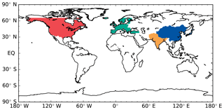
Figure 1 Emission regions according to the HTAP definition. The regions are labelled as follows: Europe (EU) is shown in green, North America (NA) is shown in red, East Asia (EA) is shown in blue and South Asia (SA) is shown in yellow.

Year 2000 is chosen as the baseline year and aerosol emissions, aerosol precursor emissions, trace gas concentrations and land use representing this year are used for the control simulation. In the emission perturbation experiments, the anthropogenic aerosol precursor emissions are decreased or increased compared to year-2000 emissions and kept constant in each region throughout the simulation. In total five coupled sensitivity experiments were performed, four experiments where SO₂ emissions were increased in the four different regions and one where anthropogenic SO₂ emissions were removed over Europe. The simulations were started from year 2000 in the transient historical CMIP5 simulation. The simulation length is 160 years for simulations where emissions are increased. For the experiment where emissions are decreased the simulation length is 200 years. All the results presented are annual mean quantities and the first 50 years of each simulation have been removed before averaging and are tested for statistical significance with Student's t test. Uncertainty ranges for the results are given as standard errors or standard deviations derived from the variability in each simulation.

The SO₂ emission changes in the emission perturbation experiments are shown in Fig. 2. In the 0×EU experiment the SO₂ emissions in Europe are not completely eliminated. There remains 4.66 Tg yr⁻¹ of volcanic emissions of SO₂ in Europe (from Etna). The SO₂ emissions in the rest of the experiments were increased by varying amounts depending on the magnitude of the regional emissions in the control simulation. This was done to obtain a global mean instantaneous radiative forcing of approximately −0.45 Wm⁻² in all these perturbation experiments. For South Asian emissions, which are low in the control simulation (6.47 Tg yr⁻¹ in year 2000 compared with 24.53 Tg yr⁻¹ in East Asia), the emissions were increased by a factor of 10. Similarly, for Europe, North America and East Asia, SO₂ emissions were increased by a factor of 7, 5 and 5, respectively.

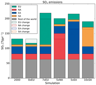
Figure 2 Global annual SO₂ and regional emissions and emission differences in the simulations. Each column shows the total global SO₂ emissions in each simulation and the colour shading indicates the contribution from each region. Hatching indicates the emission change relative to the year-2000 simulation.

The 0×EU experiment is included so that the effect of emission perturbation magnitude can be investigated, i.e. the sensitivity to a relatively small emission reduction compared to a relatively large emission increase. The emission perturbation magnitude (and sign, i.e. reduction) could also be considered as a more likely future scenario.

With the resulting global temperature response field of each emission perturbation experiment, RTP coefficients, dT_a∕dEm_r, can be constructed relating emission changes in the predefined emission regions, r, to any response region, a, of choice. The emission-based ARTP can be calculated from the absolute emission change:

$$\begin{array}{}\text{(3)}& {\displaystyle }{\mathrm{ARTP}}_{a,r}^{\mathrm{EM}}=\mathrm{\Delta }{\mathrm{Em}}_r{\displaystyle \frac{\mathrm{d}{T}_a}{{\mathrm{dEm}}_r}}.\end{array}$$

In addition to the coupled experiments we perform simulations to evaluate the instantaneous radiative forcing and effective radiative forcing of the aerosol emission perturbations in the coupled experiments.

The RF is derived from fixed sea surface temperature (SST) simulations where dual calls are made to the radiation code: one call with the CAM4 climatological aerosols and another call where the emission perturbation aerosol concentrations and their effect on cloud albedo are sent to the radiation code solely for diagnosing the radiative effect of these. Thus the meteorology in the RF simulations is identical since the radiative effects of the emission perturbations do not feed back on the meteorology. Similarly, a dual call control simulation with year-2000 aerosol emissions was performed. With this methodology the radiative effects alone from the aerosol can be quantified, without the influence of fast or slow feedbacks. The RF simulations are 7 years long and the 5 last years are used for the analysis.

The ERF is derived by performing fixed SST simulations with aerosol emission perturbations and letting the radiation changes affect the meteorology. These simulations are compared to a fixed SST simulation with year-2000 aerosol emissions. Thus, in addition to the aerosol direct radiative effect and cloud albedo effect the ERF also includes radiative changes from fast feedbacks such as cloud microphysical and semi-direct effects. In NorESM these effects include cloud liquid water content and cloud fraction. These simulations are for 20 years and the 15 last years are used for the analysis. Similarly to the coupled simulations, the RF and ERF are tested for statistical significance with Student's t test. Standard errors and standard deviations from the simulations are used to indicate the uncertainty range.

In a simplified manner, the process chain from emission to global mean temperature response can be thought of as a translation of emission to column burden, to the instantaneous direct and indirect radiative forcing, to forcing including fast feedbacks and to the full coupled temperature response. In an attempt to identify where the largest divergence appears in the process chain from emission to temperature response in the experiments conducted with NorESM, we investigate the usefulness and accuracy of alternative quantities to the unit emission in predicting the surface temperature response.

3 Results

3.1 Global forcing and temperature response

The simplest way to describe the sulfur emission perturbation impact on global and regional temperatures is to express the temperature response in terms of temperature change per unit emission of sulfur (see Sect. 2.1). We first analyse the results from the sensitivity experiments where SO₂ emissions were increased. The results from the 0×EU experiment will be discussed in Sect. 3.3. The global mean temperature response per unit emission for these sensitivity experiments where the SO₂ emissions were increased by comparable magnitudes, the global temperature change per unit emission, is similar within 10 %. The temperature response varies from −0.0056 to −0.0061 K(TgSyr⁻¹)⁻¹, depending on the location and magnitude of the sulfur emission change (Table 2).

Table 2 Global results from the experiment where SO₂ emissions in different regions are changed. Units are 10⁻²K(TgSyr⁻¹)⁻¹ for temperature change per emission change, 10⁻² Wm⁻²(TgSyr⁻¹)⁻¹ for RF and ERF per emission change and K(Wm⁻²)⁻¹ for temperature change per unit RF and ERF. Standard deviations are in parentheses.

All global mean temperature changes are significantly different compared to the temperature of the year-2000 control simulation but are not significantly different between each other (Fig. S1a in the Supplement). Thus, the location of an emission change does not appear to be a governing factor for the global mean temperature response modelled by NorESM. However, all emission changes are located in the Northern Hemisphere, and atmospheric transport of aerosol particles will contribute to a redistribution of atmospheric concentrations and the resulting column burden and radiative forcing of the aerosol, so that in some cases the resulting column burden and radiative forcing from emission changes in different regions will partly overlap.

The global average RF per unit emission change (Table 2) shows larger variability than the global temperature response (varying from −0.010 to −0.017 Wm⁻²(TgSyr⁻¹)⁻¹, with the largest RF value being 62 % larger than the smallest value), and a larger emission change is needed in EU than in SA to obtain the same RF change. The variability for the global mean ERF is similar to that of the RF (difference of 64 % between the largest and smallest value, varying from −0.008 to −0.026 Wm⁻²(TgSyr⁻¹)⁻¹) but the magnitude of the global mean ERF is smaller than the RF for all emission-increase experiments except for the 5×NA experiment. Thus, on a global scale, fast cloud feedbacks contribute to the dampening of the forcing effect of the emission increases in the NorESM experiments presented here.

3.1.1 Emission changes as a predictor of global mean temperature change

As outlined in Sect. 2, the extreme simplification inherent in the method of describing the temperature response in terms of emission perturbations leads to uncertainties related to the generality of the RTP coefficients.

Figure 3a illustrates how SO₂ emission perturbations in the different experiments translate to global sulfate column burden, RF, ERF and temperature anomalies. All values are normalised by the response in the North American experiments to illustrate the relative amount of variability for each response quantity (i.e. response in the 5×NA experiment is always 1 in Fig. 3.)

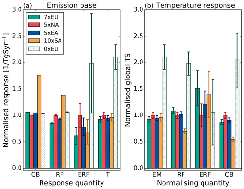
Figure 3 Normalised (a) column burden (CB), radiative forcing (RF), effective radiative forcing (ERF) and temperature (T) per unit SO₂ emission; and (b) normalised temperature response per emissions, RF, ERF and CB in the different experiments. Quantities are normalised by the 5×NA response. The error bars show the standard error.

As noted previously, the global temperature responses per unit emission in the experiments where SO₂ emissions are increased are not significantly different from each other. However, the translation from emission to column burden shows a different pattern. For this quantity, the column burden per unit emission in the 10×SA experiment is 76 % higher than in the other experiments. Thus, the geographical location seems to be one factor controlling the column burden sensitivity to emission perturbations in the experiments where emissions are increased. The increased emissions in SA together with a local SA reduction in precipitation of 0.22 mm day⁻¹ lead to a longer residence time of sulfate (0.73 days longer) as well as other aerosol particles in NorESM in the 10×SA experiment compared to the control experiment.

A similar pattern to the column burden is evident for the normalised instantaneous RF response to a unit emission change. The RF response to a unit emission change in SA is larger than the responses in the other experiments. Thus, there appears to be a close connection between changes in the global sulfate column burden and the RF. The normalised ERF sensitivity to unit emission perturbations shows a larger variability between the experiments compared to the other investigated quantities. The standard deviations for the global average ERF responses are also larger than that for RF. This result indicates that cloud feedbacks, such as changes in liquid water content or cloud fraction and cloud albedo, contribute substantially to the ERF (see Table S1 in the Supplement) and also contribute to larger variability.

Figure 3b shows the temperature response normalised by the different “basis quantities” (i.e. the leftmost group of bars in Fig. 3b are identical to the rightmost bars in Fig. 3a). The perfect basis quantity would be one for which the heights of all bars corresponding to the different experiments are equal. A basis quantity with this property would be the ideal predictor of the global mean temperature response. Figure 3b shows that emission perturbation is a good predictor of the temperature response for emission increases from all regions investigated when emissions are increased in all regions (standard deviations corresponding the each group of bars are presented in Table 3). Instantaneous RF and column burden as basis quantities underestimate the temperature response to SA emissions (this is connected to the larger column burden and RF sensitivity to a unit emission perturbation in SA which do not translate to a larger temperature sensitivity). For ERF there is substantial variability in the predictability for the temperature responses in the emission-increase experiments, which also yields the largest standard deviation of the basis quantities for these experiments.

Table 3 Standard deviations for the different normalised basis quantities evaluated in Fig. 3b (unitless).

3.2 Sub-global forcing and temperature response

3.2.1 Latitudinal forcing and temperature response

The sub-global normalised temperature responses in the experiments where SO₂ emissions were increased display more variation between the different experiments than the global mean sensitivities. (As mentioned before, the 0×EU experiment will be discussed in Sect. 3.3.2.) The latitudinal temperature responses per unit emission in the experiments with increased emissions show a qualitatively similar pattern of increasing sensitivity with increasing latitude (Fig. 4). This pattern of Arctic amplification is not dependent on the location of the emission perturbation in these experiments, neither in the latitudinal nor the longitudinal direction. The temperature responses in each latitude band are significantly different from the temperature in the year-2000 control simulation (at the 99 % confidence level), except for the Southern Hemisphere temperature responses (indicated by gray shading of the columns in Fig. 4). The latitudinal temperature responses in the different experiments are not significantly different from each other, with the exception of most of the latitudinal temperature responses to SA emissions (at the 90 % confidence level; see Fig. S1 in the Supplement for details). Thus, the latitudinal temperature responses are in principle indistinguishable for emission increases from EU, NA and EA, whereas the SA emission response is weaker in NHml and ARCT while it is stronger in SHext and the tropics compared to the other experiments. The spatial distributions of the temperature responses are shown in Fig. 5.

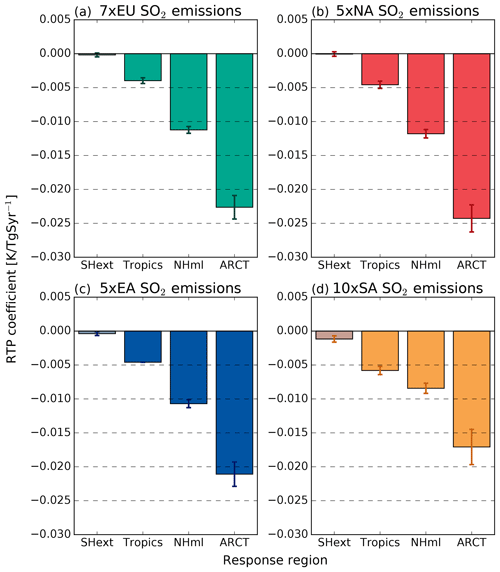
Figure 4 Latitudinal RTP coefficients for SO₂ emission K(TgSyr⁻¹)⁻¹ for (a) EU emissions, (b) NA emissions, (c) EA emissions and (d) SA emissions. Grey shading indicates that the temperature change is not statistically significant (p>0.05) compared to the control simulation. The error bars show the standard error.

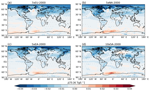
Figure 5 Global temperature change per unit SO₂ emission for (a) 7×EU, (b) 5×NA, (c) 5×EA and (d) 10×SA compared to the control simulation. Dots indicate where the result is statistically significant at the 95 % confidence level.

The only latitudinal RF and ERF that are statistically significant are the responses to emission increases in EU, NA and EA in NHml, the latitudinal band inside which these emission regions are located (Fig. 6). Significant ERF responses are also found in ARCT for the same emission source regions, but the ERF is larger in NHml, where the emissions changes are located, than in ARCT. SO₂ emission increases in SA do not lead to any latitudinal average RF or ERF responses that are statistically significant. A large fraction of the atmospheric sulfur mass from SA emissions (which are mainly emitted in the tropics) is transported to the NHml region, so that the average RF, ERF and column burden in this region exceeds that of the tropical region. However, the total integrated sulfur column burden is larger in the tropics than in the NHml (not shown) in the 10×SA experiment.

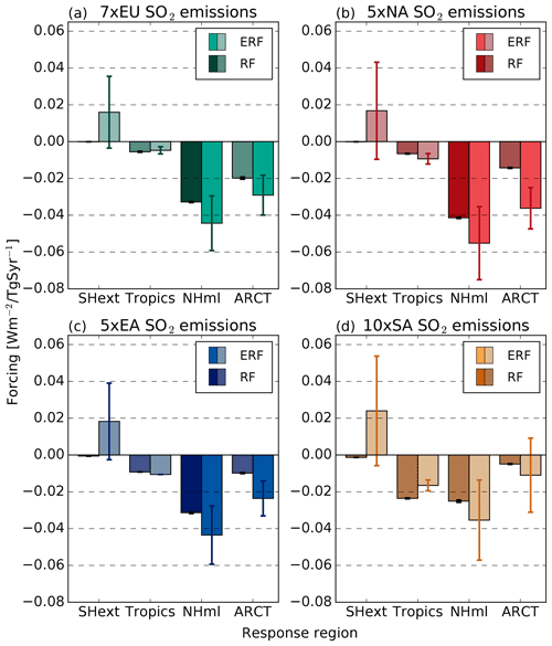
Figure 6 Latitudinal RF and ERF for SO₂ emission (Wm⁻²(TgSyr⁻¹)⁻¹) for (a) EU emissions, (b) NA emissions, (c) EA emissions and (d) SA emissions. In each pair of bars the left bar indicates RF and the right bar indicates ERF. Grey shading indicates that the forcing response is not statistically significant (p>0.05) compared to the control simulation. The error bars show the standard error.

The ERF acts to enhance the forcing relative to the RF in the NHml in all experiments, as well as in the ARCT region. This is a manifestation of aerosol indirect effects which lead to higher cloud water content (Table S1 in the Supplement). The ERF displays a warming effect in the SHext (see also Fig. 7) in all experiments (due to decreases in low cloud fraction at Southern Hemisphere mid-latitudes, not shown), although this positive ERF is not significant in any experiment. However, the positive ERF in the Southern Hemisphere, which represents a large part of the global mean, contributes to the lower value of global average of the ERF compared to the RF (see Sect. 3.1).

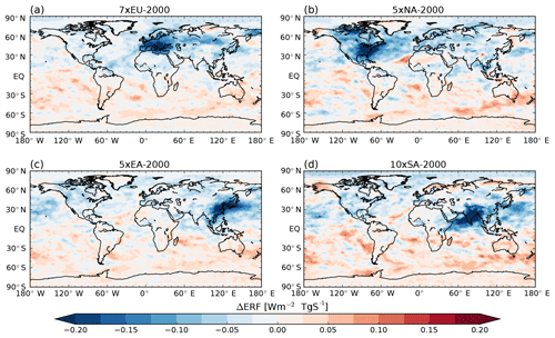
Figure 7 Global effective radiative forcing per unit SO₂ emission for (a) 7×EU, (b) 5×NA, (c) 5×EA and (d) 10×SA compared to the control simulation. Dots indicate where the result is statistically significant at the 95 % confidence level.

As described above, the temperature responses in the latitudinal bands are similar between the experiments with the exception of the temperature responses to changed SO₂ emissions in SA. SA has the largest tropical response which, however, is only significantly different from the tropical response to EU emissions, which is the weakest tropical response among the experiments. Similarly, the ARCT response to SA emissions is the smallest among the experiments, and is only significantly different to the ARCT response to NA emissions, which leads to the strongest response in ARCT. The weaker NHml response to SA emissions compared to the other emission regions, on the other hand, is significantly different compared to all other NHml temperature responses. The NA, EU and EA emission regions are for the most part located in the Northern Hemisphere mid-latitudes, and mostly north of the SA emission region. Thus, the longitudinal position of a mid-latitude emission perturbation does not appear to matter for the latitude mean temperature responses at Northern Hemisphere high and mid-latitudes.

3.2.2 Regional temperature response

The differences between the sub-global temperature responses in the different experiments become more evident when they are derived for the emission perturbation regions (and the AR region north of 66^∘ N) compared to when derived for latitudinal bands (Fig. 8). All regional temperature changes are statistically significant compared to the control simulation. The largest temperature response is found in the AR region in all experiments, which is consistent with the latitudinal distribution of the temperature response for latitude bands described in the previous section. Similarly, the SA emissions have the smallest effect on the AR temperature among the experiments, but the AR temperature response in this experiment is only significantly different from the response to NA emissions, which give the largest AR response among the experiments.

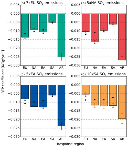
Figure 8 Regional RTP coefficients for SO₂ emission (K(TgSyr⁻¹)⁻¹) for (a) EU emissions, (b) NA emissions, (b) EA emissions and (d) SA emissions. Grey shading indicates that the temperature change is not statistically significant (p>0.05) compared to the control simulation. The error bars show the standard error. Black dots indicate the zonal mean for the latitudes that cover each region.

Outside the AR region, the largest temperature response is found locally in the emission region in all experiments except 10×SA. This result is consistent with the forcing always being largest in the emission region (Fig. 9). The regional RF and ERF is also statistically significant for local SO₂ emissions from SA, as opposed to when derived for the tropical latitudinal band (Fig. 6). For SA emissions the temperature response in the EA region is marginally larger than the local temperature response in the SA region. The EA region is located downwind of the SA region, which means that a substantial part of the sulfur emitted in SA is transported to EA and contributes to the local forcing in EA. The column burden increases by 3 %(TgSyr⁻¹)⁻¹ in EA due to SA emission, which compares with the increase in EA due to local emission of 4 %(TgSyr⁻¹)⁻¹. Additionally, advection of air originating from SA might also partly explain the large temperature response in the EA region to SA emissions. EA is the only region where there are emissions from a remote region (SA) that lead to a temperature response that is indistinguishable from the effect of local emissions.

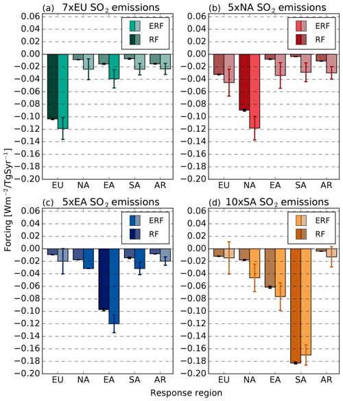
Figure 9 Regional RF and ERF for SO₂ emission (Wm⁻²(TgSyr⁻¹)⁻¹) for (a) EU emissions, (b) NA emissions, (c) EA emissions and (d) SA emissions. In each pair of bars the left bar indicates RF and the right bar indicates ERF. Grey shading indicates that the forcing response is not statistically significant (p>0.05) compared to the control simulation. The error bars show the standard error.

The local temperature responses in the emission perturbation regions are larger than the corresponding zonal mean temperature responses of the latitudes covered by each region (indicated by black dots in Fig. 8) in all experiments. The largest local response relative to the zonal mean is found in the 10×SA experiment, which is 66 % larger than the zonal mean. The 5×NA experiment shows the largest absolute difference between the local response and the zonal mean, 0.0055 K(TgSyr⁻¹)⁻¹ (55 % larger). The smallest local temperature response relative to the zonal mean is found for 7×EU (20 %). All differences between these local responses and the corresponding zonal means are statistically significant at the 95 % confidence level.

For both NA and EU emission perturbations, the temperature responses in the regions outside the emission regions are close to the corresponding zonal mean responses (within 2 %–17 % difference). SA and EA emission perturbations, on the other hand, both lead to a larger temperature response than the corresponding zonal mean for NA and a smaller temperature response than the zonal mean for EU, where both of these differences between the zonal mean and regional temperature response are statistically significant. Both EA and SA emission perturbations have a substantial effect on NA temperature, of the same magnitude as the local responses for these emission regions, despite the geographical distance between the emission location and the temperature response regions. Local radiative forcing in NA is not responsible for this temperature effect (Fig. 9). This result points towards a far field effect in the temperature response to Asian aerosol forcing which is mediated by atmospheric circulation changes rather than radiation changes.

3.3 Non-linearities

So far, only the results from the experiments where SO₂ emissions were increased have been discussed. In this section we will focus on the differences between the results from the 0×EU and 7×EU SO₂ emission changes experiments. The purpose is to investigate if the emission perturbation magnitude or background state influences the temperature response (see e.g. Wilcox et al., 2015).

3.3.1 Global temperature response

In the experiment where European anthropogenic SO₂ emissions are removed, the global average temperature change per unit emission is approximately twice that in the 7×EU experiment, as well as in the other experiments where emissions were increased (Fig. 3 and Table 2). The global average temperature change per unit emission in the emission reduction experiment is significantly different from those in the emission-increase experiments (Fig. S1 in the Supplement). This indicates that there is a non-linearity depending on the magnitude and sign of the emission change, at least for European SO₂ emissions. Since the coupled simulations include aerosol indirect effects, and since indirect effects are usually larger than direct aerosol effects (Rap et al., 2013; Myhre et al., 2013; Kirkevåg et al., 2013), non-linear effects pertaining to aerosol–cloud interactions most likely play a role in the difference in global climate sensitivity between the 0×EU and 7×EU experiments. However, effects related to the modelled aerosol microphysics could also play a role in this difference, in particular when SO₂ emissions and concentrations are low. For example, in extreme conditions the partitioning between different aerosol microphysical paths might change, like condensation and nucleation rates of sulfate (Stier et al., 2006).

The two experiments with different European SO₂ emission perturbations illustrate the difficulties related to the generality of the method of translating emission perturbations to temperature response already discussed in Sect. 3.1. The global mean temperature responses per unit sulfur emission differ substantially for these two experiments, as well as the magnitudes of the latitudinal and regional temperature responses.

We return to the question of basis quantities (see Sect. 3.1) and for which step in the translation from emission to temperature response the largest divergence appears for the different experiments. The normalised global temperature responses per unit emission in the experiments where SO₂ emissions are increased are close to unity, while the normalised temperature response per unit emission in the 0×EU experiment is larger than two (Fig. 3). The translation from emission to column burden for the EU emission changes is not dependent on the emission magnitude in the experiments presented here. Similar to what was noted for the other experiments, the RF per unit emission change in 0×EU and 7×EU is similar to the column burden response per unit emission change. The normalised ERF sensitivity to unit emission perturbation, on the other hand, bears more resemblance to the temperature response for the 0×EU and 7×EU experiments (third group of bars/the next rightmost bars in Fig. 3a). This indicates that fast cloud feedbacks, such as cloud lifetime, liquid water content or semi-direct effects, are most likely a key component for understanding the non-linearity in the temperature response to European emissions (see Tables S1 and S2 in the Supplement).

Emission perturbation was in Sect. 3.1 found to be a good predictor of the temperature response for emission increases from all regions investigated when the emissions were increased with similar magnitudes. However, it does not capture the non-linear behaviour in the temperature response to European emission perturbations of different magnitudes (Fig. 3b). Similarly, RF and column burden as basis quantities also fail to capture this property in the response to European emission perturbations. The ERF is the only basis quantity that captures the non-linearity for European emission perturbations of varying magnitude. However, there is substantial variability in the predictability for the temperature responses in the other experiments. The ERF shows the smallest standard deviation for the different basis quantities when all experiments are considered (Table 3), but this is due to substantially larger standard deviations for emissions, CB and RF as basis quantities when the 0×EU experiment is included. Nevertheless, the ERF is the basis quantity with the highest degree of generality for the global results from all the experiments conducted with NorESM presented in this study.

3.3.2 Sub-global temperature response

Similarly to the global mean response, the magnitude of the latitudinal and regional temperature responses per unit sulfur emission is substantially larger in the 0×EU experiment than in the 7×EU experiment, with the exception of the temperature difference in SA which is not statistically significant compared to the control simulation (Fig. 10, where hatched bars indicate the 7×EU response for easy comparison). For the latitudinal sensitivities, the pattern of increasing temperature response with latitude found in the experiments where emissions were increased (Sect. 3.2.1 and Fig. 4) is also seen for the 0×EU experiment. The relative impact on the Southern Hemisphere is also larger in this experiment compared to the other experiments. All latitudinal temperature changes in the 0×EU experiment are significantly different from the responses in all the other experiments except for the tropical latitude band (Fig. S1 in the Supplement).

Figure 10 Latitudinal (a) and regional (b) RTP coefficients for 0×EU SO₂ emissions (K(TgSyr⁻¹)⁻¹). Grey shading indicates non-statistical differences (p>0.05). The hatching indicates the RTP for 7×EU emissions (cf. Figs. 4 and 8) for easy comparison. The error bars show the standard error.

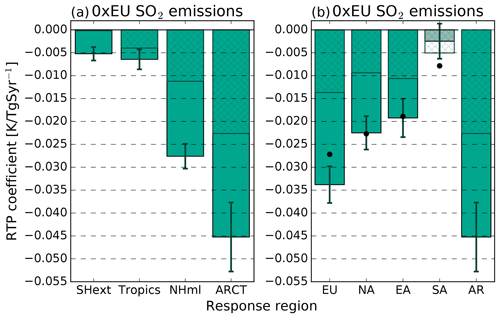
The regional 0×EU responses display a similar pattern to the regional responses in the 7×EU experiment but with different magnitudes. The largest temperature response is seen in the AR region, whereas outside AR the largest response is found in the emission region (EU). The temperature responses to reduced EU SO₂ emissions in NA and EA are close to the zonal means for the latitudes covered by these regions (within 2 %). This is similar to the corresponding regional temperature responses in the 7×EU experiment relative to the zonal mean responses.

The non-linear effects are mostly confined to the magnitude of the temperature responses in the case of European emission perturbations in these experiments. Zonal asymmetries do not appear to have a significant impact on the regional temperature responses. This might, however, be different for the Asian emission perturbations where zonal asymmetries seem to play a more prominent role in the regional temperature distributions compared to the European and North American emission perturbations.

3.4 Comparison with other RTP coefficients

In this work we have aimed to establish the simplest possible model for anthropogenic aerosol impacts on regional temperatures, i.e. an emission-based regional temperature potential coefficient.

Nevertheless, difficulties associated with non-linear effects in this relationship remain where ERF proved to be a more general basis quantity for estimating the global temperature response than emissions, in terms of capturing different magnitudes of global mean temperature responses for different emission changes in Europe.

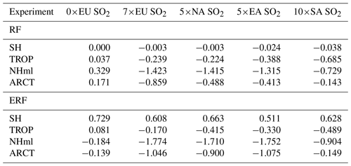
With the experimental set-up applied in this study, it is not possible to derive sub-global (latitudinal or regional) radiative-forcing-based sensitivities, as the forcing changes in the different experiments are not confined to a certain region or latitude band. However, with the latitudinal and regional RF and ERF from the different experiments, the generality of the RTP coefficients derived by Shindell and Faluvegi (2009) and Shindell (2012) can be assessed for the NorESM-generated temperature response. For each experiment the RF and ERF in each latitude band resulting from the regional emission perturbations are calculated (Table 4) and used with different methods for calculating the latitudinal temperature responses, the ARTP.

Table 4 Regional radiative forcing (RF) and effective radiative forcing (ERF) in Wm⁻² used to derive latitudinal ARTPs in Figs. 11–14.

First we compare the temperature response as calculated from Eqs. (1) and (2) with that from the simulations with NorESM where SO₂ emissions were increased. Both equations require knowledge of the model global climate sensitivity (or the impulse response function). The climate sensitivities are derived from the emission perturbation experiments, and we use a mean value from all experiments with emission increases. Climate sensitivities for both RF and ERF are derived, and these are calculated to be 0.47 and 0.61 K(Wm⁻²)⁻¹, respectively.

However, the model global climate sensitivity is not always known, e.g. if the forcing is derived with a chemical transport model. Moreover, one motivation behind using RTP coefficients is to avoid conducting multi-century coupled simulation, which is necessary for deriving the climate sensitivity. Therefore, we also evaluate the performance of the RTP coefficients with a standardised climate sensitivity as well as apply the RTP coefficients of Shindell and Faluvegi (2010) as regional sensitivity coefficients (i.e. without normalising with the regional climate sensitivity to global forcing and scaling with the model's global sensitivity). This is to see how well the RTP method predicts the model temperature response when the specific model's climate sensitivity to a particular forcing agent is unknown.

The latitudinal temperature responses calculated from Eqs. (1) and (2) are shown in Figs. 11 and 12. The small dots indicate the temperature response in specific regions and the filled circles indicate the emission source regions. The high-latitude temperature response in the Northern Hemisphere (ARCT) calculated using the RTP coefficients, the ARTP, is underestimated compared to the temperature response in the NorESM experiments (but still within 1 standard deviation of the NorESM simulated temperature response), except for when the ERF is used in combination with the normalised coefficients of Shindell et al. (2012) (Fig. 12b). This is also the method that gives the smallest root mean square deviation (RMSD) of 0.14 K (RMSDs are displayed in each panel). In general, ERF is a better predictor of the latitudinal temperature response than RF, based on the RMSD. Similarly, the RTP coefficients that are normalised by the global sensitivity (Shindell et al., 2012) rather that the regional sensitivity (Shindell and Faluvegi, 2010), i.e. Fig. 11 vs. Fig. 12, are a better model for the temperature response in each latitude band, also based on the RMSD. This was also pointed out by Shindell (2012).

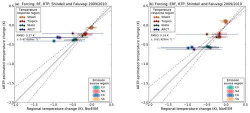
Figure 11 Regional temperature change from the coupled simulations (horizontal axis) compared with the estimated temperature response when using (a) RF and (b) ERF in combination with the RTP coefficients of Shindell and Faluvegi (2009), Eq. (1) with the climate sensitivity derived from the current experiments (vertical axis). The horizontal bars indicate 1 standard deviation for the temperature response in the coupled simulations. The dashed lines show a ±20 % agreement threshold.

Figure 12 As Fig. 11 but with the RTP coefficients of Shindell (2012), Eq. (2) with the climate sensitivity derived from the current experiments.

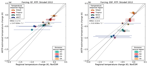
However, the performance of this method relies on the correct climate sensitivity being used and known. The standard definition of equilibrium climate sensitivity (ECS) is the equilibrium temperature response to a doubling of CO₂ (Collins et al., 2013) and is available for nearly all models participating in the Coupled Model Intercomparison Project Phase 5 (Flato et al., 2013). For NorESM this climate sensitivity has been estimated to 0.91 K(Wm⁻²)⁻¹ (Iversen et al., 2013, λ_reg in Table 1). This is higher than the sensitivity to aerosol forcing obtained in this study. The climate sensitivity from the simulations presented here is not directly comparable with an equilibrium climate sensitivity, since an equilibrium temperature response would require considerably longer simulations for allowing the ocean to fully adjust. The results of the RTP method with this ECS applied are shown in Fig. 13. Overall, the use of ECS overestimates the temperature response in almost all latitude bands. Thus, it is important to use a climate sensitivity appropriate for the timescale investigated and possibly also for the particular climate forcer in question. This is a complicating factor since it requires a priori knowledge of this quantity, which can only be derived by performing coupled simulations, the necessity of which one often would like to eliminate with a simplified method. Moreover, if calculations to derive radiative forcing are performed with a CTM, this quantity is not available.

Figure 13 As Fig. 11 but with the RTP coefficients of Shindell (2012), Eq. (2) with the CO₂ sensitivity from Iversen et al. (2013).

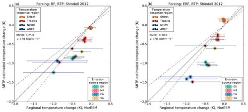
A third alternative is to apply the RTP coefficients without normalising with a model-dependent climate sensitivity parameter, i.e. using the RTP coefficients of Shindell and Faluvegi (2010), Table 3, directly with forcing estimates (Fig. 14). The implicit assumption in this method is that the sensitivity of NorESM to aerosol forcing is equal to that of the GISS model simulations used to derive the RTP coefficient. This is equivalent to applying the GISS model's sensitivity of 0.5 K(Wm⁻²)⁻¹ (Shindell, 2012) in Eq. (2). This assumption about the sensitivity leads to RTP-derived temperature responses with smaller RMSD values than both of those derived by applying the ECS for NorESM in Eqs. (1) and (2).

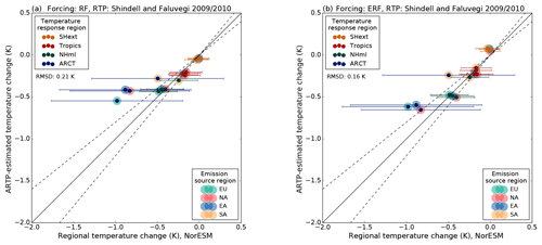
Figure 14 As Fig. 11 but with the RTP coefficients of Shindell and Faluvegi (2009), and with no climate sensitivity applied.

4 Discussion

4.1 Uncertainties associated with RTP coefficients

The method applied in this work, i.e. evaluating the global and regional temperature responses based on the emission change magnitudes, means that, on the one hand, the starting quantity is easy to assess and compare and is easy to incorporate into integrated assessment models, such as GAINS. The full response chain from emissions to atmospheric concentrations, to forcing and to surface temperature response is accounted for in this metric. On the other hand, the fact that the metric encompasses the full chain from emission to temperature response means that there are implicit uncertainties in the metric. The representativeness of these emission-based RTP coefficients will depend on how well the climate model used to derive these coefficients represents a large number of atmospheric chemical and physical processes on many different spatial and temporal scales. The RTP coefficients derived by Shindell and Faluvegi (2009) and Shindell (2012) were derived from radiative forcing and thus do not contain the uncertainties introduced when estimating the column burden and forcing associated with aerosol emissions. However, a model to translate emission to radiative forcing, either RF or ERF, is still necessary to make these forcing-based RTP coefficients useful in an integrated assessment modelling context based on emission pathways.

Some major uncertainties can be identified if the emission–temperature response chain is broken down into sub-steps. First, emissions of an atmospheric chemical compound result in an atmospheric concentration and column burden. The translation from emission of an atmospheric chemical component to atmospheric aerosol loading depends on a number of factors, e.g. if the aerosol originates from primary emission or is formed through chemical reactions in the atmosphere (i.e. secondary aerosols), like sulfate which is studied here. The aerosol production for secondary aerosols will depend on which and how chemical reactions that produce these aerosols are described in the atmospheric model. Kasoar et al. (2016) found that the efficiency of chemical conversion of SO₂ to sulfate was one process contributing to differences in the simulated responses in three different climate models to equivalent emission reductions over China. In addition to chemical production, the interaction with clouds will influence the atmospheric concentration of aerosols. Wet removal through precipitation is an efficient removal process for hygroscopic aerosols like sulfate-containing compounds. All these factors, emission strength, atmospheric production and removal efficiency influence how long aerosol particles stay in the atmosphere and how far they are transported from the emission sources. Thus, all these processes influence the atmospheric loading, and how these processes are represented in the model will influence the modelled aerosol column burden.

Another source of uncertainty in the emission–forcing–temperature chain, besides the modelled column burden, is how the aerosol radiative properties are modelled (Myhre et al., 2013). The radiative properties of aerosols depend on their chemical composition, water content and mixing state. Thus, given the same atmospheric concentration and distribution of aerosols, their radiative effect might vary depending on how their radiative properties are represented in the model. Other complicating factors when it comes to aerosol radiative effects are clouds and aerosol indirect and semi-direct effects on clouds. The direct radiative forcing will depend on the cloud distribution itself, and aerosol can affect the properties of clouds and also affect the cloud distribution; i.e. other components, besides the aerosol itself, within the model influence their radiative effects (Stier et al., 2013).

One of the largest uncertainties associated with the effect of aerosols on climate is related to their indirect effect on clouds (Myhre et al., 2013) and the representation of these can vary widely between different models. Besides chemical conversion and radiative impacts, Kasoar et al. (2016) also identified indirect effects on clouds as a major source of diversity between the models they investigated. Wilcox et al. (2015) found that parameterisations of the relationship between cloud droplet number concentration and effective radius were the largest contribution to differences in the cloud albedo effect between three models from the CMIP5 archive, among those NorESM.

The factors described above all contribute to inter-model diversity and will influence how general RTP coefficients are across models. However, the same processes also contribute to regional sensitivity differences within the same model, not based on differences in how the processes are represented in the model but on the specific meteorological conditions in each region (e.g. cloud climatology, regional circulation patterns and the background aerosol).

The results presented in this study indicate that the temperature sensitivity depends on the emission change magnitude in NorESM. The global temperature response per unit SO₂ emission in the EU SO₂ removal experiment is approximately twice that in the EU SO₂ increase experiment, although the results are also associated witch large uncertainties. The non-linearity in the response appears to belong to aerosol interactions with clouds and in particular to fast feedbacks included in the ERF. These include changes in liquid water content, cloud fraction and subsequent changes in cloud albedo of the new cloud distribution, i.e. cloud lifetime effects (Albrecht, 1989) (the cloud albedo effect of the background cloud distribution is included in RF).

Wilcox et al. (2015) derived simple functional forms representing the relationship between sulfate load and cloud droplet effective radius (i.e. the cloud albedo effect) in three different CMIP5 models, with which they could reproduce the time evolution of the simulated cloud droplet effective radius from historical 20th century simulations. With these functional forms, they could also quantify (i) the intrinsic varying sensitivity in the parameterisation of the effective radius which depends on the magnitude of the sulfate load and (ii) how the effective radius (and ultimately radiative forcing) goes from being highly sensitive at low sulfate loads to a relative insensitive state at high sulfate loads. While they focussed on the cloud albedo effect, the cloud lifetime effect is a direct consequence of initial change in effective radius and should thus display a similar varying sensitivity depending on the absolute sulfate load.

Thus, the similarity of the global temperature responses in the emission-increase experiments, despite different mechanisms, might be due to this saturation of cloud droplet effective radius change when emission increases are large enough. The temperature sensitivity for the different regions could prove to be different if emission were reduced, even by equivalent amounts, depending on the regional background emission strength and regional meteorological conditions. Non-linear effects depending on the emission change magnitude and background are one of the biggest hurdles in creating a general emission-based RTP coefficient.

4.2 Basis quantity

Different quantities for predicting the temperature response have been assessed for the global mean temperature and for latitudinal bands in combination with the RTP coefficients of Shindell and Faluvegi (2010) and Shindell (2012). In both cases ERF proved to have the best skill for predicting the temperature response.

For the global mean temperature response, the ERF was the only variable that was capable of capturing the large difference in the temperature responses to the European increase and decrease in SO₂ emissions. However, for the emission-increase experiments, emission change was a good predictor for temperature change. Also for the latitudinal ARTPs the ERF performed better in predicting temperature responses than the RF for NorESM, which is mostly due to a simulated larger ERF than RF in the Arctic region. This can either be an indication that the sensitivity of the Arctic region to forcing outside the Arctic region is larger in NorESM than GISS, i.e. that the coefficient relating the forcing to Arctic temperature responses should be larger for NorESM. It could also be an indication that the cloud feedbacks in the Arctic are a necessary part of the forcing and that the local forcing from fast feedbacks is important for the Arctic response in NorESM.

4.3 Latitudinal and regional sensitivities

The sensitivity of zonal mean temperatures to emission perturbations in different regions shows large similarities, with the exception of the overall weaker Northern Hemisphere temperature response to SA SO₂ emissions; the zonal mean temperature changes increase with increasing latitude in all experiments and do not appear to depend strongly on the location of the emission perturbations within the Northern Hemisphere (Fig. 4). There are many factors that might contribute to the weaker temperature response to the SA emission perturbation. This emission perturbation is located in one of the major monsoonal regions on the globe, and the increase in sulfate leads to a substantial reduction of precipitation over SA (Tables S1 and S2 in the Supplement). The reduced precipitation, in turn, leads to less efficient wet removal of aerosol, resulting in an increased residence time and a larger column burden response per unit emission of both sulfate and BC compared to the control simulation. The decrease in precipitation in SA (as well as smaller increases in liquid water path, Tables S1 and S2 in the Supplement) also contributes to a weaker ERF and indirect effect on clouds, which in the other experiments enhances the local forcing, but not in SA (Fig. 9). This result is one example of how different local meteorological conditions where the emission changes occur contribute to different forcing and temperature responses within the same model.

The general pattern, which indicates a stronger temperature response with increasing latitude for all emission perturbations, is a robust feature in all experiments. In all experiments, the second largest regional sensitivity (after the Arctic region) is generally found in the region of the emission perturbation. However, for SA emissions, the sensitivity is slightly larger in the East Asian region compared to the South Asian emission region, a result caused by production of sulfate aerosol from SO₂ and subsequent transport from SA to EA. These results are in line with those of Conley et al. (2018), who found a similar latitudinal temperature change distribution in three different models in response to removal of US SO₂ emissions, and Kasoar et al. (2018), who conducted a single model study where they found that the Arctic warmed most in response to removal of SO₂ emissions in different regions.

Moreover, Asian SO₂ emissions, both from EA and SA, produce larger zonal asymmetries in the global temperature change field than those of EU and NA. The Asian SO₂ emissions lead to temperature responses in NA and EU that are higher and lower, respectively, than the zonal mean response. The remote regional temperature responses to EU and NA SO₂ emissions are on the other hand close to the corresponding zonal mean responses. The location in the Asian monsoon region and proximity to the western Pacific mean that these SO₂ emissions could cause tropical precipitation changes that are effective in generating planetary-scale waves. These waves can propagate into the extratropics, which in turn influences the global temperature distribution (Ming et al., 2011; Lewinschal et al., 2013). Moreover, Teng et al. (2012) found a temperature impact in North America directly linked to absorbing aerosols in Asia.

However, the standard deviations for the regional sensitivities are larger than those for the latitudinal sensitivities and zonal mean sensitivities. Nevertheless, despite the larger uncertainties associated with the regional RTPs compared to the latitudinal RTPs, they provide information that is not captured by the latitudinal RTPs.

5 Summary and conclusions

We performed simulations with the Earth system model NorESM to evaluate the surface temperature change in response to SO₂ emission perturbations in Europe, North America, and East and South Asia and to derive emission-based RTP coefficients. Four experiments were performed where emissions were increased relative to the year 2000 in each individual region to yield similar global mean radiative forcing values. One additional experiment was performed where anthropogenic SO₂ emissions were completely removed in Europe.

In all five experiments the zonal mean latitudinal temperature change distribution showed a similar pattern of increasing temperature change with increasing latitude, independently of where the emission perturbation was located. The largest temperature response in all experiments performed was in this study thus found in the Arctic region, regardless of where the emission perturbations were located, similarly to the result of Conley et al. (2018) and Kasoar et al. (2018). Outside the Arctic region, the temperature response was largest in the emission perturbation region, except for SA emissions where the temperature response in the neighbouring EA region was equally large. This result was consistent with the radiative forcing pattern, which was also strongest in the emission region in each experiment.

Furthermore, indications were found that the emission-based RTPs derived with NorESM might be non-linear. Removal of anthropogenic European SO₂ emissions led to a temperature response per unit emission approximately twice that in the 7×EU experiment in NorESM. The result is, however, associated with large uncertainties. Other differences were also noticed for the regional responses to regional emission perturbations. Asian emission increases led to a different remote effect compared to increases in EU and NA emissions. Both EA and SA emission perturbations led to an NA temperature response that was larger than the zonal mean and an EU response that was smaller than the corresponding zonal mean. EU and NA emission perturbations, on the other hand, led to remote responses that were close to the zonal mean for the same latitudes.

A comparison of the modelled temperature response in NorESM with that calculated using ARTPs (Eqs. 1 and 2) derived with the RTP coefficients of Shindell and Faluvegi (2010) and Shindell (2012) showed that the RTP coefficients predict similar latitudinal temperature change distributions to those produced by NorESM. The agreement between the calculated values using ARTPs and the temperature change simulated using NorESM was better when ERF was used together with the RTP coefficient than when RF was used. This was mainly due to a larger Arctic ERF than RF that resulted in an Arctic temperature response closer to that produced in the NorESM simulations. This result could be an indication that the Arctic is more sensitive to forcing outside this region in NorESM than in the GISS model or that local fast cloud feedbacks are crucial for the Arctic temperature response in NorESM.

Even though the global mean temperature response to emission increases is similar in all regions, the processes leading to the change may be different in different regions, as they depend on the local meteorological conditions. In all regions except SA, aerosol indirect effects on clouds, and particularly lifetime effects, dominate the ERF response. For SA, direct radiative effects have a higher relative importance in the response since the local responses in cloud fraction, liquid water path and precipitation are either weaker compared to the other emission regions or decrease in response to increased SO₂ emissions. The latitudinal distribution of the zonal mean temperature response to SA emission changes also differs from the rest of the simulations in that the Northern Hemisphere response is weaker and the Southern Hemisphere and tropical responses are stronger than in the other simulations.

Air pollution globally causes more than four million premature deaths each year, and as sulfates are major air-pollution components, emission reductions of SO₂ will be absolutely necessary to improve air quality. The derived emission-based RTPs will simplify the development of cost-effective co-beneficial abatement strategies that can give both better air quality and mitigate climate change. The non-linear effect predicted by NorESM indicates a reduced immediate climate effect of SO₂ emission reductions in highly polluted areas where the indirect effect is saturated but the effect would become more evident with time as the saturation of aerosol indirect effects diminishes. Nevertheless, emission reductions of SO₂ and other short-lived climate forcers are necessary for improving air quality and public health in both Europe, North America and Asia.