Exploiting multi-wavelength aerosol absorption coefficients in a multi-time resolution source apportionment study to retrieve source-dependent absorption parameters

In this paper, a new methodology coupling aerosol optical and chemical parameters in the same source apportionment study is reported. In addition to results on source contributions, this approach provides information such as estimates for the atmospheric absorption Ångström exponent (α) of the sources and mass absorption cross sections (MACs) for fossil fuel emissions at different wavelengths.

A multi-time resolution source apportionment study using the Multilinear Engine (ME-2) was performed on a PM₁₀ dataset with different time resolutions (24, 12, and 1 h) collected during two different seasons in Milan (Italy) in 2016. Samples were optically analysed by an in-house polar photometer to retrieve the aerosol absorption coefficient b_ap (in Mm⁻¹) at four wavelengths (λ=405, 532, 635, and 780 nm) and were chemically characterized for elements, ions, levoglucosan, and carbonaceous components. The dataset joining chemically speciated and optical data was the input for the multi-time resolution receptor model; this approach was proven to strengthen the identification of sources, thus being particularly useful when important chemical markers (e.g. levoglucosan, elemental carbon) are not available. The final solution consisted of eight factors (nitrate, sulfate, resuspended dust, biomass burning, construction works, traffic, industry, aged sea salt); the implemented constraints led to a better physical description of factors and the bootstrap analysis supported the goodness of the solution. As for b_ap apportionment, consistent with what was expected, biomass burning and traffic were the main contributors to aerosol absorption in the atmosphere. A relevant feature of the approach proposed in this work is the possibility of retrieving a lot of other information about optical parameters; for example, in contrast to the more traditional approach used by optical source apportionment models, here we obtained source-dependent α values without any a priori assumption (α biomass burning =1.83 and α fossil fuels =0.80). In addition, the MACs estimated for fossil fuel emissions were consistent with literature values.

It is worth noting that the approach presented here can also be applied using more common receptor models (e.g. EPA PMF instead of multi-time resolution ME-2) if the dataset comprises variables with the same time resolution as well as optical data retrieved by widespread instrumentation (e.g. an Aethalometer instead of in-house instrumentation).

1 Introduction

Atmospheric aerosol impacts on both local and global scale, causing adverse health effects (Pope and Dockery, 2006), decreasing visibility (Watson, 2002), and influencing the climate (IPCC, 2013). To face these issues an accurate knowledge of aerosol emission sources is mandatory.

Currently, multivariate receptor models are considered a robust approach (Belis et al., 2015) for performing source apportionment studies, and positive matrix factorization (PMF) (Paatero and Tapper, 1994) has become one of the most widely used receptor models (Hopke, 2016) in the aerosol community. In the late 1990s, the Multilinear Engine (ME-2) was developed and proven to be a very flexible algorithm to solve multilinear and quasi-multilinear problems (Paatero, 1999). The scripting feature of this algorithm allows the implementation of advanced receptor modelling approaches; one example is the multi-time resolution model (Zhou et al., 2004), which uses each experimental datum in its original time schedule as model input. Source apportionment studies carried out by multi-time resolution models are still scarce in the literature (Zhou et al., 2004; Ogulei et al., 2005; Kuo et al., 2014; Liao et al., 2015; Crespi et al., 2016; Sofowote et al., 2018), although this methodology is very useful in measurement campaigns when instruments with different time resolutions (minutes, hours, or days) are available as high time resolution data can be exploited without averaging them over the longest sampling interval.

It is noteworthy that the combination of time-resolved chemically speciated data with the information obtained from instrumentation measuring aerosol optical properties at different wavelengths (e.g. the absorption coefficient b_ap) is suggested as one of the future investigations of receptor modelling (Hopke, 2016); however, to the best of our knowledge, very few attempts in this direction have been made (e.g. Peré-Trepat et al., 2007; Xie et al., 2019). Wang et al. (2011, 2012) in a source apportionment study used the Delta-C (Delta-C = BC@370–BC@880 nm from Aethalometer measurements) as an additional input variable and found that Delta-C was very useful in separating traffic from biomass burning source contributions.

The wavelength dependence of b_ap can be empirically considered to be proportional to λ^−α, where α is the absorption Ångström exponent; α depends on particle composition and size, and it is a useful parameter to gain information about particle type in the atmosphere (see e.g. Yang et al., 2009). Among aerosol components, black carbon (BC) is the main factor responsible for light absorption in the atmosphere; in fact, it is considered the main aerosol contributor to global warming and the second most important anthropogenic contributor after CO₂ (Bond et al., 2013). Black carbon refers to a fraction of the carbonaceous aerosol characterized by peculiar features as for microstructure, morphology, thermal stability, solubility, and light absorption (Petzold et al., 2013); in particular, it is characterized by a wavelength-independent imaginary part of the refractive index over visible and near-visible regions. Another aerosol-absorbing component is brown carbon (BrC), referred to as light-absorbing organic matter with increasing absorption towards shorter wavelengths, especially in the UV region (Andreae and Gelencsér, 2006). BrC is an aerosol component that also affects the elemental vs. organic carbon correct separation when using thermal-optical methods as outlined by Massabò et al. (2016).

Source apportionment models based only on multi-wavelength b_ap data are available in the literature, i.e. the widespread Aethalometer model (Sandradewi et al., 2008a) and the more recent Multi-Wavelength Absorption Analyzer (MWAA) model (Massabò et al., 2015; Bernardoni et al., 2017b). Briefly, these models estimate the source contributions to aerosol absorption, exploiting their different dependence on λ (i.e. different α). As a step forward, MWAA provides the b_ap apportionment in relation to both the sources (i.e. fossil fuel combustion and biomass burning) and the components (i.e. BC and BrC), and also provides an estimate for α of BrC. Indeed, source apportionment models based on optical data usually assume two contributors to b_ap, namely fossil fuel combustion and biomass burning (only a few exceptions are present in the literature, e.g. Fialho et al., 2005). In most cases this assumption is well founded, except when episodic events giving a non-negligible contribution to aerosol absorption in the atmosphere occur, such as in the presence of mineral dust from the Sahara Desert (Fuzzi et al., 2015). Moreover, the above-mentioned models need a priori assumptions about the α values of the sources and wide ranges for α are reported in the literature (e.g. Sandradewi et al., 2008a); this is the most critical step, since α depends on fuel type, burning conditions and aging processes in the atmosphere. Without accurate determination of source-specific atmospheric α (for example exploiting the information derived from source apportionment using ¹⁴C measurements), the applicability of models based on optical data is questionable (Bernardoni et al., 2017b; Massabò et al., 2015; Zotter et al., 2017). Moreover, the generally accepted assumption of α=1 for fossil fuels and BC, arising from the theory of absorption by spherical particles in the Rayleigh regime (Seinfeld and Pandis, 2006), might not always be valid for aged atmospheric aerosol (Liu et al., 2018).

In the framework of a source apportionment study based on multi-time resolution receptor modelling, optical and chemical datasets were joined to retrieve a multi-λ apportionment of b_ap, with no need for a priori assumptions about the contributing sources. Instead of using α as an a priori input, as far as we know here for the first time, this approach directly provided source-dependent α values. Moreover, the multi-λ apportionment of b_ap in each source allowed us to estimate MAC values at different wavelengths, exploiting the well-known relation EBC=b_ap(λ)/MAC(λ) (Bond and Bergstrom, 2006) where elemental carbon (EC) apportioned by the model was considered to be a proxy for BC. The evaluation of atmospheric MAC values is also not trivial due to the possible presence of absorbing components different from BC (e.g. contribution from BrC, especially at shorter wavelengths).

The original approach proposed in this work shows that coupling the chemical and optical information in a receptor modelling process is particularly advantageous because (1) it strengthens the source identification that is particularly useful when relevant chemical tracers (e.g. levoglucosan, EC) are not available; (2) it gives estimates for source-specific atmospheric α values which are typically assumed a priori in source apportionment models based on optical data; and (3) it provides MAC values at different wavelengths for specific sources.

In this work, optical data were measured by an in-house multi-wavelength polar photometer and input data (chemical + optical) in the receptor model comprised variables acquired with different time resolutions. Anyway, it is worth noting that the approach presented here is of general interest as the same methodology could be applied to (1) datasets combining aerosol chemical and optical data obtained by widespread instrumentation (e.g. Aethalometers for optical data) and (2) variables with the same time resolution.

2 Material and methods

2.1 Site description and aerosol sampling

Two measurement campaigns were performed during summertime (June–July) and wintertime (November–December) 2016 in Milan (Italy). Milan is the largest city (more than 1 million inhabitants, doubled by commuters everyday) of the Po Valley, a very well-known hotspot pollution area in Europe due to both large emissions from a variety of sources (i.e. traffic, industry, domestic heating, energy production plants, and agriculture) and low atmospheric dispersion conditions (e.g. Vecchi et al., 2007, 2019; Perrone et al., 2012; Bigi and Ghermandi, 2014; Perrino et al., 2014).

The sampling site is representative of the urban background and it is situated at about 10 m above the ground, on the roof of the Physics Department of the University of Milan, less than 4 km from the city centre (Vecchi et al., 2009). It is important to note that during the sampling campaigns, a large building site was active next to the monitoring station.

Aerosol sampling was carried out using instrumentation with different time resolutions. Low time resolution PM₁₀ data, with sampling durations of 24 and 12 h during summertime (20 June–22 July 2016) and wintertime (21 November–22 December 2016), respectively, were collected in parallel on PTFE (Whatman, 47 mm diameter) and pre-fired (700 ^∘C, 1 h) quartz-fibre (Pall, 2500QAO-UP, 47 mm diameter) filters. Low-volume samplers with EPA PM₁₀ inlet operating at 1 m³ h⁻¹ were used. High time resolution data were collected during shorter periods (11–18 July and 21–28 November 2016) by a streaker sampler (D'Alessandro et al., 2003). Briefly, the streaker sampler collects the fine and coarse PM fractions (particles with aerodynamic diameter d_ae < 2.5 µm, and 2.5 < d_ae < 10 µm, respectively) with hourly resolution. Particles with d_ae > 10 µm impact on the first stage and are discarded; the coarse fraction deposits on the second stage, consisting of a Kapton foil; finally, the fine fraction is collected on a polycarbonate filter. The two collecting supports are kept in rotation with an angular speed of about 1.8^∘ h⁻¹ to produce a circular continuous deposit on both stages.

Meteorological data were available at a monitoring station belonging to the regional environmental agency (ARPA Lombardia) which is less than 1 km away.

2.2 PM mass concentration and chemical characterization

In this section, chemical analyses performed on samples are summarized. As concentration detected in each sample was characterized by its own uncertainty, only ranges for experimental uncertainties and minimum detection limits (MDLs) for every set of variables are reported.

PM₁₀ mass concentration was determined on PTFE filters by a gravimetric technique. Weighing was performed by an analytical balance (Mettler, model UMT5, 1 µg sensitivity) after a 24 h conditioning period in an air-controlled room as for temperature (20±1 ^∘C) and relative humidity (50±3 %) (Vecchi et al., 2004).

These filters were then analysed by energy dispersive X-ray fluorescence (ED-XRF) analysis to obtain the elemental composition (details on the procedure can be found in Vecchi et al., 2004). For most elements and samples, concentrations were characterized by relative uncertainties in the range 7 %–20 % (higher uncertainties for elements with concentrations next to MDLs) and minimum detection limits of 0.9–30 ng m⁻³ with the above-mentioned sampling conditions.

For each quartz-fibre filter, one punch (1.5 cm²) was extracted by sonication (1 h) using 5 mL ultrapure Milli-Q water and levoglucosan and inorganic anions concentrations were quantified. Levoglucosan concentration was determined by high-performance anion exchange chromatography coupled with pulsed amperometric detection (HPAEC-PAD) (Piazzalunga et al., 2010) only in winter samples. Indeed, as already pointed out by other studies at the same sampling site (Bernardoni et al., 2011) and routinely assessed at monitoring stations in Milan by the Regional Environmental Agency (private communication), levoglucosan concentrations during summertime are lower than the MDLs (i.e. about 6 ng m⁻³), due to both lower emissions (no influence of residential heating and negligible impact from other sources) and higher OH levels in the atmosphere depleting molecular marker concentrations (Robinson et al., 2006; Hennigan et al., 2010). Uncertainties on levoglucosan concentration were about 11 %. The quantification of the main water-soluble inorganic anions (${\mathrm{SO}}_{\mathrm{4}}^{\mathrm{2}-}$ and ${\mathrm{NO}}_{\mathrm{3}}^{-}$) was performed by ion chromatography (IC); MDLs were 25 and 50 ng m⁻³ with summertime and wintertime sampling conditions, respectively, and uncertainties were about 10 %. Unfortunately, due to technical problems, no data on ammonium were available. Details on the analytical procedure for IC analysis are reported in Piazzalunga et al. (2013).

Another punch (1.0 cm²) of each quartz-fibre filter was analysed by thermal optical transmittance analysis (TOT, Sunset Inc., NIOSH-870 protocol) (Piazzalunga et al., 2011) in order to assess organic and elemental carbon (OC and EC) concentrations. MDLs were 75 and 150 ng m⁻³ with summertime and wintertime sampling conditions, respectively, and uncertainties were in the range 10 %–15 %.

Hourly elemental composition was assessed by the particle-induced X-ray emission (PIXE) technique, using a properly collimated proton beam and scanning the deposits in steps corresponding to 1 h aerosol deposit (details in Calzolai et al., 2015). As low time resolution PM₁₀ samples were also available, fine and coarse elemental concentrations determined by PIXE analysis were added up to obtain PM₁₀ concentrations with hourly resolution. PM₁₀ hourly concentrations for most elements and samples were characterized by relative uncertainties in the range 10 %–30 % (higher uncertainties for elements near MDLs) and MDLs ranged from a minimum of 0.1 to a maximum of 15 ng m⁻³ (higher MDLs typically detected for Z < 20 elements).

2.3 Aerosol light-absorption coefficient measurements

The aerosol absorption coefficient (b_ap) at the four wavelengths λ=405, 532, 635, and 780 nm was measured on both low and high time resolution samples with the in-house polar photometer PP_UniMI (Vecchi et al., 2014; Bernardoni et al., 2017c).

Low time resolution optical measurements taken into account were those performed on PTFE filters since their physical characteristics can be considered more similar to polycarbonate filters used by the streaker sampler. Moreover, previous works reported a bias on b_ap measured by instrumentation using fibre filters (e.g. Cappa et al., 2008: Lack et al., 2008; Davies et al., 2019, and references therein). Vecchi et al. (2014) found that b_ap at 635 nm was 40 % higher when measured on a quartz-fibre filter compared to parallel samples collected on PTFE. This effect was ascribed to sampling artefacts due to organics in aerosol samples collected in Milan.

As for high time resolution samples, b_ap was measured only in the fine fraction collected on polycarbonate filters since absorption of the Kapton foil on which the coarse fraction was collected did not allow b_ap assessment. Anyway, b_ap values in PM_2.5 and PM₁₀ were expected to be fairly comparable, as aerosol absorption in the atmosphere is mostly due to particles in the fine fraction at heavily polluted urban sites like Milan. To verify this assumption, high time resolution b_ap data in PM_2.5 were averaged over the timescale of low time resolution b_ap in PM₁₀ and compared; the agreement was good, between 11 % and 13 % depending on the λ, except for b_ap at λ=405 nm that showed a higher difference (27 %) but with most data (83 %) within experimental uncertainties. To take into account this difference, b_ap data at λ=405 nm were homogenized before using them in the model, following the criterion used for chemical species (for further details about the homogenization procedure, see Sects. 2.4 and 2.5).

Uncertainties on b_ap were quantified in 15 % and MDL was in the range 1–10 Mm⁻¹ depending on sampling duration and wavelength as already reported in Vecchi et al. (2014) and Bernardoni et al. (2017c). The pre-treatment procedure for experimental uncertainties and MDLs was the same used for chemical variables in order to create suitable input matrices required by the multi-time resolution model (see also Sect. 2.5). Optical system stability was checked during the measurement session, evaluating the reproducibility of the measurement on a blank test filter. Laser stability was also checked at least twice a day and the recorded intensities were used to normalize blank and sampled filter analysis.

2.4 Model description

Multivariate receptor models (Henry, 1997) are among the most widespread and robust approaches used to perform source apportionment studies for atmospheric aerosol (Belis et al., 2014, 2015). In particular, positive matrix factorization PMF2 (Paatero and Tapper, 1994; Paatero, 1997) had been extensively used in the literature and, afterwards, the Multilinear Engine ME-2 (Paatero, 1999, 2000) introduced the possibility of solving all kinds of multilinear and quasi-multilinear problems. The fundamental principle of these modelling approaches is the mass conservation between the emission source and the receptor site; using the information carried by aerosol chemical composition assessed in samples collected at the receptor site, a mass balance analysis can be performed to identify the factors influencing aerosol mass concentrations (Hopke, 2016). Factors can be subsequently interpreted as the main sources impacting the site, through the knowledge about major sources in the investigated area and the exploitation of chemical fingerprints available from previous literature works (Belis et al., 2014). Referring to the input data as matrix X (matrix elements x_ij), the chemical profile of the factors as matrix F (matrix elements f_kj), and the time contribution of the factors as matrix G (matrix elements g_ik), the main equation of a bilinear problem can be written as follows:

$$\begin{array}{}\text{(1)}& x_{ij}=\sum _{k=\mathrm{1}}^P{g}_{ik}{f}_{kj}+e_{ij},\end{array}$$

where the indices i, j, and k indicate the sample, the species, and the factor, respectively; P is the number of factors and the matrix E (matrix elements e_ij) is composed of the residuals, i.e. the difference between measured and modelled values.

In this way, a system of N×M equations is established, where N is the number of samples and M is the number of species. The solution of the problem is computed by minimizing the object function Q defined as

$$\begin{array}{}\text{(2)}& Q=\sum _{i=\mathrm{1}}^N\sum _{j=\mathrm{1}}^M{\left({\displaystyle \frac{e_{ij}}{{\mathit{\sigma }}_{ij}}}\right)}^{\mathrm{2}},\end{array}$$

where σ_ij are the uncertainties related to the input data.

The multi-time resolution receptor model was developed in order to use each data value in its original time schedule, without averaging the high time resolution data or interpolating the low time resolution data (Zhou et al., 2004; Ogulei et al., 2005). The main Eq. (1) is consequently modified as below:

$$\begin{array}{}\text{(3)}& x_{sj}={\displaystyle \frac{\mathrm{1}}{t_{s\mathrm{2}}-t_{s\mathrm{1}}+\mathrm{1}}}\sum _{k=\mathrm{1}}^P{f}_{kj}\sum _{i=t_{s\mathrm{1}}}^{t_{s\mathrm{2}}}{g}_{ik}{\mathit{\eta }}_{jm}+e_{sj},\end{array}$$

where the indices s, j, and k indicate the sample, the species, and the factor, respectively; P is the number of factors; t_s1 and t_s2 are the starting and ending times for the sth sample in time units (i.e. the shortest sampling interval that is 1 h for the dataset used here); and i represents one of the time units of the sth sample. η_jm are adjustment factors for chemical species replicated with different time resolution and measured with different analytical methods (represented by the subscript m).

If η is close to unity, species concentration measured by different analytical approaches can be considered in good agreement; non-replicated species have adjustment factors set to unity by default. In this work, the adjustment factors were always set to unity in the model; to take into account the use of two types of aerosol samplers (i.e. low-volume sampler with EPA inlet and streaker sampler) and different analytical techniques to obtain the elemental composition (i.e. ED-XRF and PIXE), concentrations of replicated species with multiple time resolutions were homogenized before inserting them into the input matrix X, as will be explained in Sect. 2.5. This data treatment avoids the consistency check between η values calculated by the model and differences in experimental data characterized by high and low time resolution. Otherwise, this step should always be performed after running the model.

In the multi-time resolution model the following regularization equation is introduced to take into account that some sources could contain few or no species measured with high time resolution:

$$\begin{array}{}\text{(4)}& g_{(i+\mathrm{1})k}-g_{ik}=\mathrm{0}+{\mathit{\epsilon }}_i,\end{array}$$

where ε_i represent the residuals.

As already pointed out by Ogulei et al. (2005), a weighing parameter for species might be necessary; in this study, it was implemented in the equations and set at 0.5 for strong species (not applied to weaker species such as Na, Mg, and Cr; see Sect. 2.5) in 24 or 12 h samples.

Equations (3) and (4) are solved using the Multilinear Engine (ME) program (Paatero, 1999). In Eq. (2), the object function Q takes into account residuals from the main Eq. (3) and from the auxiliary equations (regularization Eq. 4, normalization equation, pulling equations, and constraints).

In this work, the multi-time resolution model implemented by Crespi et al. (2016) was used; therefore, constraints were inserted into the model and the bootstrap analysis was also performed to evaluate the robustness of the final solution.

2.5 Input data

As already mentioned in Sect. 2.4, instead of using adjustment factors in the model (all set equal to one), concentrations of replicated species with different time resolutions were pre-homogenized and then inserted into the input matrix X. Concentration data with longer sampling intervals (24 and 12 h in this work) were considered to be the benchmark, since analytical techniques usually show a better accuracy on concentration values far from MDLs (i.e. samples collected on longer time intervals) (Zhou et al., 2004; Ogulei et al., 2005).

Variables were then classified as weak and strong according to the signal-to-noise ratio (S/N) criterion (Paatero, 2015). For hourly data only strong variables (S/N ≥1.2) were considered; for low time resolution data weak variables such as Na, Mg, and Cr (with S/N equal to about 0.8) being strong variables in hourly samples were also included, although with associated uncertainties comparable to concentration values in order to avoid the exclusion of too many data. Indeed, excluding these low time resolution variables from the analysis gave rise to artificial high values in the time contribution matrix for sources traced by these species (in this case it was an issue for aged sea salt traced by Na and Mg; see Sect. 3.2); this oddity was already reported by Zhou et al. (2004).

Every measured variable in each sample is characterized by its own uncertainty; ranges of experimental uncertainties and MDLs are reported in Sects. 2.2 and 2.3 for chemical and optical analyses, respectively. Variables with more than 20 % of the concentration data below MDL values were omitted from the analysis (Ogulei et al., 2005). Uncertainties and data below minimum detection limits were pre-treated according to Polissar et al. (1998). In general, missing concentration values were estimated by linear interpolation of the measured data and their uncertainties were assumed to be 3 times this estimated value (Zhou et al., 2004; Ogulei et al., 2005). As for summertime levoglucosan data (always below MDLs), the approach was to include them as below-MDL data and not as missing data following Zhou et al. (2004), who underlined that the multi-time resolution model is more sensitive to missing values than the original PMF model. In order to avoid double counting, in this study S was chosen as the input variable instead of ${\mathrm{SO}}_{\mathrm{4}}^{\mathrm{2}-}$ as it was determined on both low time and high time resolution samples (by XRF and PIXE analysis, respectively; see Calzolai et al., 2008). However, elemental ${\mathrm{SO}}_{\mathrm{4}}^{\mathrm{2}-}$ and S concentrations showed a high correlation (correlation coefficient R=0.98) and the Deming regression gave a slope of 2.69±0.13 (sulfate vs. sulfur) with an intercept of $-\mathrm{198}\pm \mathrm{82}$ ng m⁻³, i.e. compatible with zero within 3 standard deviations. The slight difference (of the order of 10 %) between the estimated slope and the ${\mathrm{SO}}_{\mathrm{4}}^{\mathrm{2}-}$-to-S stoichiometric coefficient (i.e. 3) can be ascribed to either a small fraction of insoluble sulfate or to the use of different analytical techniques.

PM₁₀ mass concentrations were included in the model with uncertainties set at 4 times their values (Kim et al., 2003). In the end, 22 low time resolution variables (PM₁₀ mass, Na, Mg, Al, Si, S, K, Ca, Cr, Mn, Fe, Cu, Zn, Pb, EC, OC, levoglucosan, ${\mathrm{NO}}_{\mathrm{3}}^{-}$, b_ap 405 nm, b_ap 532 nm, b_ap 635 nm, b_ap 780 nm) and 17 hourly variables (Na, Mg, Al, Si, S, K, Ca, Cr, Mn, Fe, Cu, Zn, Pb, b_ap 405 nm, b_ap 532 nm, b_ap 635 nm, b_ap 780 nm) were considered.

The input matrix X consisted of 386 samples and the total number of time units was 1117. The analysis was performed in the robust mode; the lower limit for G contribution was set to −0.2 (Brown et al., 2015) and the error model em$=-\mathrm{14}$ was used for the main equation with C₁= input error, C₂=0.0, and C₃=0.1 (Paatero, 2012) for both chemical and optical absorption data.

Sensitivity tests on the uncertainty of absorption data were performed starting from a minimum experimental uncertainty of 10 %. Lower uncertainties were considered not physically meaningful from an experimental point of view. ME-2 analyses performed with 10 % experimental uncertainty on absorption data gave very similar results to the base-case solution presented in the Supplement (Fig. S1 and Table S3 in the Supplement), with no differences in mass apportionment and a maximum variation in the concentrations of chemical and optical profiles (matrix F) of 7 % when considering significant variables in each profile (i.e. explained variation for matrix F EVF higher or near 0.30). In contrast, considering an experimental uncertainty of 20 % on absorption data, the solution significantly differed from the one reported in the Supplement and showed less physical meaning (e.g. a couple of factors got mixed, or an additional unique factor appeared giving a null mass contribution). Thus, the estimated relative experimental uncertainty of 15 % was here considered appropriate for optical variables.

It is also noteworthy that ME-2/PMF analysis is not a priori harmed by the use of joint matrices containing different dimensions/units (see e.g. Paatero, 2018). Indeed, if different units are present in different columns of matrix X, the output data in the factor matrix G are pure numbers and elements in a column of the factor matrix F carry the same dimension and unit as the original data in matrix X. In addition, the average total contribution to the mass of a specific source due to species in a certain factor in matrix F must be retrieved a posteriori by summing up only mass contributions by chemical components (i.e. excluding optical components in matrix F).

To the authors' knowledge, this was the first time that the absorption coefficient at different wavelengths was introduced in the multi-time resolution model jointly with chemical variables and used to more robustly identify the sources; moreover, this approach led to the assessment of source-dependent α and MAC values in an original way.

3 Results and discussion

3.1 Concentration values

In Table S1 basic statistics on mass and chemical species concentrations at different time resolutions are given.

Most variables showed higher mean and median concentrations during the winter campaign, when atmospheric stability conditions influenced the monitoring site; exceptions were Al, Si and Ca, which had lower median concentrations (as detected in low time resolution samples). This was not unexpected as they are typical tracers of soil dust resuspension (Viana et al., 2008) that can be more relevant during summertime due to drier soil conditions and stronger atmospheric turbulence. Moreover, the good correlation between these elements (Al vs. Si: R²=0.94 and Ca vs. Si: R²=0.78) suggested their common origin.

Potassium showed the clearest seasonal behaviour in concentration values going from 284 ng m⁻³ (10th–90th percentile: 151–344 ng m⁻³) to 660 ng m⁻³ (10th–90th percentile: 349–982 ng m⁻³) in summer and winter, respectively, in low time resolution samples. K is an ambiguous tracer, since it is emitted by a variety of sources, among which there are crustal resuspension and biomass burning. In our dataset, wintertime K values showed a good correlation with levoglucosan concentrations (R²=0.71), suggesting the impact of biomass burning as levoglucosan is a well-known tracer for biomass burning emissions in winter samples (Simoneit et al., 1999). Also looking at the K-to-Si ratio (where Si was taken as a soil dust marker), significant seasonal differences came out; it was 0.35±0.15 in high time resolution summer samples and 2.0±2.2 in winter ones, to be compared with the much more stable Al-to-Si ratio (i.e. 0.26±0.04 and 0.28±0.09 in summer and winter, respectively) indicating a soil-related origin.

Among the elements typically associated with anthropogenic sources, Fe and Cu showed a good correlation (e.g. R²=0.72 on hourly resolution samples) as well as Cu and EC (Cu vs. EC: R²=0.84, on low time resolution data); in addition, the diurnal pattern of Fe and Cu showed traffic rush-hour peaks (07:00–09:00 LT and around 19:00 LT as shown in Fig. 1). These results were suggestive of a common source; in the literature these aerosol chemical components are reported as tracers for vehicular emissions (e.g. Viana et al., 2008; Thorpe and Harrison, 2008).

In Table S2 basic statistics on b_ap values referring to low-resolution samples collected on PTFE are also reported. Diurnal mean temporal patterns for b_ap at different wavelengths (retrieved from hourly resolved data) are displayed in Fig. 2.

Figure 1 Diurnal profile of Fe and Cu concentrations (in ng m⁻³).

Figure 2 Diurnal profile of the aerosol absorption coefficient (in Mm⁻¹) measured at different wavelengths.

3.2 Source apportionment with the multi-time resolution model

Different solutions (from 5 to 10 factors) were explored; after 30 convergent runs, the eight-factor base-case solution corresponding to the lowest Q value (2086.88) was firstly selected (see Fig. S1). It is important to note that the model was run using all variables (chemical + optical) as explained in Sect. 2.5. A lower or higher number of factors caused ambiguous chemical profiles and the physical interpretation suggested clearly mixed sources for a lower number of factors or unique factors in case of more factors (i.e. Pb for nine factors); moreover, inconsistent mass closure was detected by increasing the number of factors (e.g. the sum of species contribution was up to 25 % higher than the mass for the 10-factor solution). In the eight-factor base-case solution, the mass was well reconstructed by the model (R²=0.98), with a slope of 0.98±0.02 and a negligible intercept (0.51±0.89 µg m⁻³).

The factor-to-source assignment was based on both EVF values – which are typically higher for chemical tracers (Lee et al., 1999; Paatero, 2010) – and the physical consistency of factor chemical profiles. In the chosen solution, the unexplained variation was lower than 0.25 for all variables. The uncertainty-scaled residuals (Norris et al., 2014) showed a random distribution of negative and positive values in the ±3 range, with a Gaussian shape for most of the variables (Fig. S2).

Using EVF and chemical profiles reported in Fig. S1a, the eight factors were tentatively assigned to nitrate, sulfate, resuspended dust, biomass burning, construction works, traffic, industry, and aged sea salt. In Table S3 absolute and relative average source contributions to PM₁₀ mass are reported.

Table 1 Absolute and relative average source contributions to PM₁₀ mass in the eight-factor constrained solution.

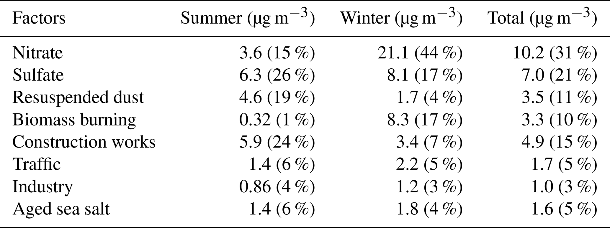
Although the above-mentioned base-case solution was a satisfactory representation of the main sources active in the area (as reported in previous works; see e.g. Marcazzan et al., 2003; Vecchi et al., 2009, 2018; Bernardoni et al., 2011, 2017a; Amato et al., 2016), the chemical profiles of some factors were improved by exploring rotated solutions. The most relevant case was represented by aged sea salt where typical diagnostic ratios such as Mg∕Na and Ca∕Na (in bulk seawater equal to 0.12 and 0.04, respectively, as reported e.g. in Seinfeld and Pandis, 2006) were not well reproduced in the base-case solution and the chemical profile was too much impacted by the presence of Fe compared to bulk seawater composition. Therefore, the above-mentioned diagnostic ratios were here used as constraints and Fe was maximally pulled down in the chemical profile. The effective increase in Q was about 61 units (Q=2147), with a percentage increase of about 3 %; as a rule of thumb, an increase in the Q value of a few tens is generally considered acceptable (Paatero and Hopke, 2009). It is noteworthy that the constrained solution led to an improvement in the chemical profile of the aged sea salt, and negligible differences in all other relevant features of the solution (i.e. EVF, residuals, mass reconstruction, source apportionment) were found compared to the base-case solution. Therefore, the eight-factor constrained solution was considered the most physically reliable; results are presented in Table 1 and Fig. 3 and discussed in detail in the following.

The factor interpreted as nitrate fully accounted for the explained variation of ${\mathrm{NO}}_{\mathrm{3}}^{-}$. This factor contained a significant fraction of nitrate in the chemical profile (39 %) and all nitrate was present only in this factor. This source was by far the most significant one at the investigated site, explaining about 31 % of the PM₁₀ mass over the whole campaign (a similar estimate – 26 % – was reported by Amato et al. (2016) during the AIRUSE campaign in Milan in 2013) increasing up to 44 % during wintertime (comparable to the 37 % reported by Vecchi et al., 2018). Indeed, the Po Valley is well known for experiencing very high nitrate concentrations during wintertime (Vecchi et al., 2018, and references therein) because of large emissions of gaseous precursors related to urban and industrial activities, residential heating, high ammonia levels due to agricultural field manure and poor atmospheric dispersion conditions.

The factor associated with sulfate showed EVF =0.47 for S and much lower EVF for all the other variables in the factor. Considering the sulfur contribution in the chemical profile in terms of ammonium sulfate, the relative contribution of sulfur components in the profile increased from 11 % (S) up to 45 % (ammonium sulfate). The latter is the main sulfur compound detected in the Po Valley as reported in previous papers such as Marcazzan et al. (2001) and was by far the highest contributor in the chemical profile. The other important contributor was OC (19 %), whose impact on PM mass increased up to 30 % when reported as organic matter using 1.6 as the organic carbon-to-organic matter conversion factor for this site (Vecchi et al., 2004). Due to the secondary origin of the aerosol associated with this factor, it was not surprising to also find a significant OC contribution; indeed, aerosol chemical composition in Milan is impacted by highly oxygenated components due to aging processes favoured by strong atmospheric stability (Vecchi et al., 2018, 2019). In this factor, EC contributed about 1 %. Considering the total EC concentration reconstructed by the model, the EC fraction related to the sulfate factor was about 6 %. In contrast to sulfates, EC has a primary origin; however, its presence with a very similar percentage (4 %–5 %) in a sulfate chemical profile was previously pointed out in Milan, indicating a more complex mixing between primary and secondary sources (Amato et al., 2016), e.g. with sulfate condensation on primary emitted particles. The sulfate factor accounted for 21 % of the PM₁₀ mass.

The factor identified as resuspended dust was mainly characterized by high EVF and contributions coming from Al, Si and Mg, i.e. crustal elements. The Al∕Si ratio was 0.31, very similar to the literature value for average crustal composition (Mason, 1966); the relatively high OC contribution in the chemical profile (15 %) together with the presence of EC (about 2.6 %) was suggestive of a mixing with road dust (Thorpe and Harrison, 2008). This source explained for about 11 % of the PM₁₀ mass.

The factor identified as biomass burning was characterized by high EVF for levoglucosan (0.98), a known tracer for this source as it is generated by cellulose pyrolysis; EVF higher than 0.3 was also found for K, OC, and EC. In the source chemical profile, OC contributed 54 %, EC 10 %, levoglucosan 7 %, and K 5 %. The average biomass burning contribution during this campaign was 10 % (up to 17 % in wintertime). Anticipating the discussion presented in detail in Sect. 3.3, it is worth noting that the second largest contribution to the aerosol absorption coefficient after traffic was detected in this factor.

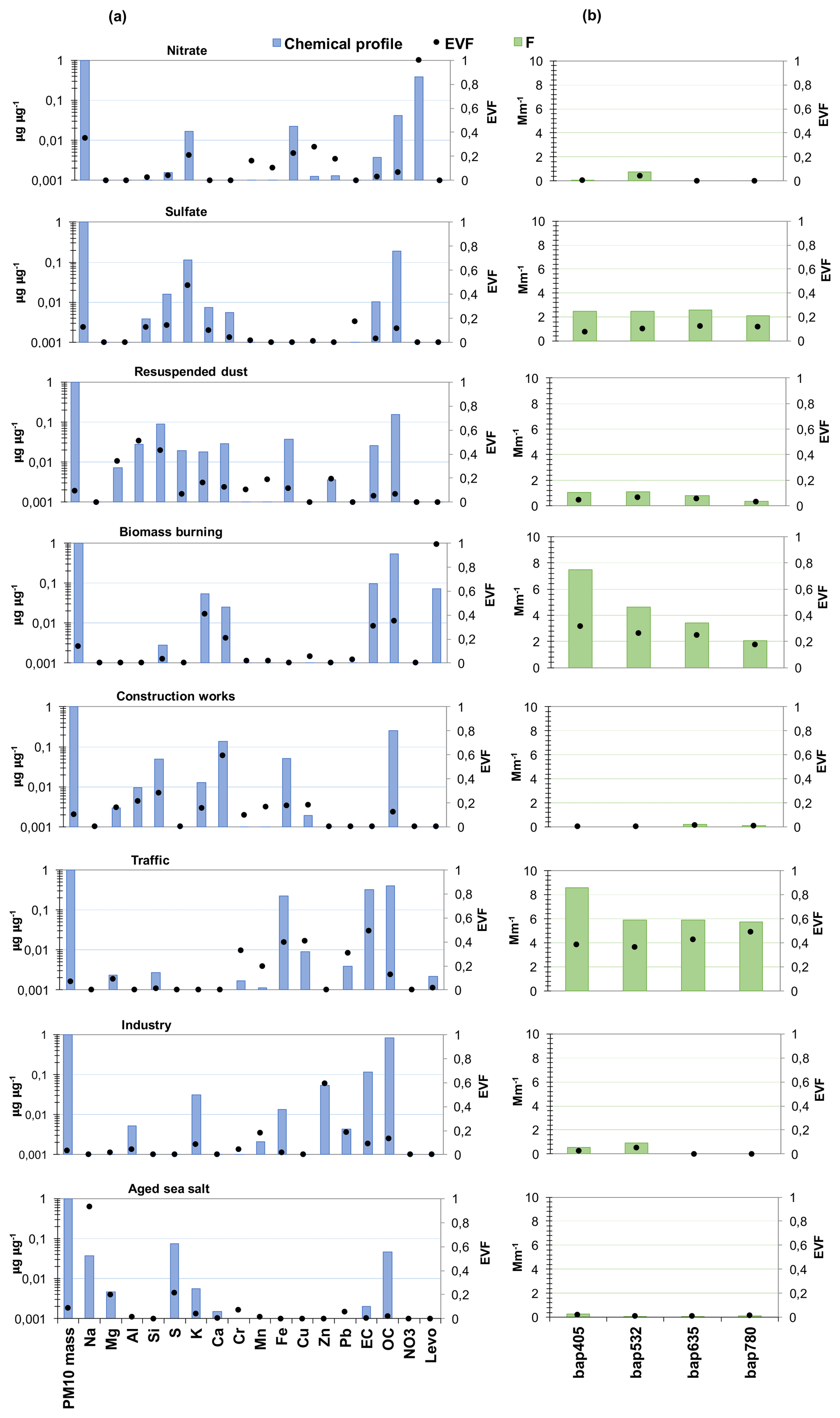
Figure 3 (a) Chemical profiles of the eight-factor constrained solution; (b) b_ap apportionment of the eight-factor constrained solution. The blue bars represent the chemical profile (output of the matrix F normalized on mass), the green bars the output values of the matrix F for the optical variables, and the black dots the EVF.

The factor with high EVF (0.60) for Ca was associated with construction works, following literature works (e.g. Vecchi et al., 2009; Bernardoni et al., 2011, 2017a; Dall'Osto et al., 2013; Crilley et al., 2017, and references therein). Major contributors to the chemical profile were Ca (13 %), OC (26 %), Fe, and Si (5 % each). This factor accounted on average for 15 % to PM₁₀ mass. As already mentioned, during the campaign a non-negligible contribution from this source was expected, due to the presence of a building site nearby the monitoring location.

In the factor assigned to traffic (primary contribution), EVF larger than 0.3 characterized EC, Cu, Fe, Cr, and Pb. The highest relative mass contributions in the chemical profile were given by OC (41 %), EC (32 %), Fe (23 %), and Cu (1 %). The lack of relevant crustal elements such as Ca and Al in the chemical profile suggested a negligible impact of road dust in this factor. As reported above, at our sampling site the road dust contribution was very likely mixed to resuspended dust and further separation of these contributions was not possible. This traffic (primary) contribution over the whole dataset accounted for 5 % of the PM₁₀ mass, with a slightly lower absolute contribution in summer (see Table 1). This contribution is comparable to the percentage (7 %) reported by Amato et al. (2016) for exhaust traffic emissions, but it is lower than our previous estimates (Bernardoni et al., 2011; Vecchi et al., 2018), i.e. 15 % in 2006 in PM₁₀ and 12 % in PM₁ recorded in winter 2012. However, the current estimate seems to still be reasonable when considering the efforts made in recent years to reduce vehicles' exhaust particle emissions and the fraction of secondary nitrate due to high nitrogen oxides and ammonia emissions in the region (INEMAR ARPA-Lombardia, 2018), which has to be added to account for the overall traffic impact. Unfortunately, the non-linearity of the emission-to-ambient concentration level relationship and the high uncertainties in emission inventories still prevent a robust estimate of this secondary contribution to total traffic exhaust emissions. As shown in Sect. 3.3, traffic is the largest contributor to the aerosol absorption coefficient, thus strengthening the interpretation of this factor as a traffic emission source.

The industry factor showed high EVF for Zn (0.59) and the second highest EVF was related to Mn (0.13). Previous studies at the same sampling site identified these elements as tracers for industrial emissions (e.g. Vecchi et al., 2018, and references therein). The chemical profile was enriched by heavy metals and, after traffic, it was the profile with the highest share of Cr, Mn, Fe, Cu, Zn, and Pb (explaining about 8 % of the total PM₁₀ mass in the profile). The industry contribution was not very high in the urban area of Milan, accounting for 3 % on average.

The factor interpreted as aged sea salt was characterized by high EVF of Na (0.93) and this element was – as a matter of fact – present only in this factor chemical profile. To check the physical consistency of this assignment and considering that Milan is about 120 km away from the nearest sea coast, back-trajectories coloured by the aged sea salt concentration (in ng m⁻³) were calculated through the NOAA HYSPLIT trajectory model (Draxler and Hess, 1998; Stein et al., 2015; Rolph et al., 2017) and represented using R package Openair (Carslaw and Ropkins, 2012; R Core Team, 2019). As an example, results from a very short event (13 July 16:00–18:00 LT) singled out by the model and representing the highest sea salt contribution during summer are reported in Fig. S3. Before and during the event, south-western air masses coming from the Ligurian Sea were observed, while soon after the event, there was a rapid change in wind direction. High wind speeds were recorded during the episode (4.8±1.7 m s⁻¹ with a maximum peak of 9.5 m s⁻¹) compared to the 1.9±1.0 m s⁻¹ average wind speed characterizing the summer campaign.

When marine air masses are transported to polluted sites, sea salt particles show a Cl deficit due to reactions with sulfuric and nitric acid (Seinfeld and Pandis, 2006) and the factor chemical profile is expected to be enriched in sulfate and nitrate. In this work, nitrate was not present in the aged sea salt chemical profile; a very rough estimate (Lee et al., 1999) gave a maximum expected contribution of 2 % (about 82 ng m⁻³) of the total nitrate mass in the atmosphere that can be considered negligible in terms of mass contribution of the sources.

Temporal patterns of Cl concentrations (not inserted in the multi-time resolution analysis as being a weak variable) during marine aerosol episodes were exploited to further confirm the factor-to-source association. Cl concentration and aged sea salt pattern showed an evident temporal coincidence in peak occurrence during the short summer event (Fig. 4), thus supporting the source identification. Moreover, during this episode only the Cl coarse fraction increased (Fig. S4) and reached about 90 % of the total PM₁₀ Cl concentration; the Cl∕Na ratio was 0.38±0.05, consistent with an aging of marine air masses during advection showing the typical Cl depletion.

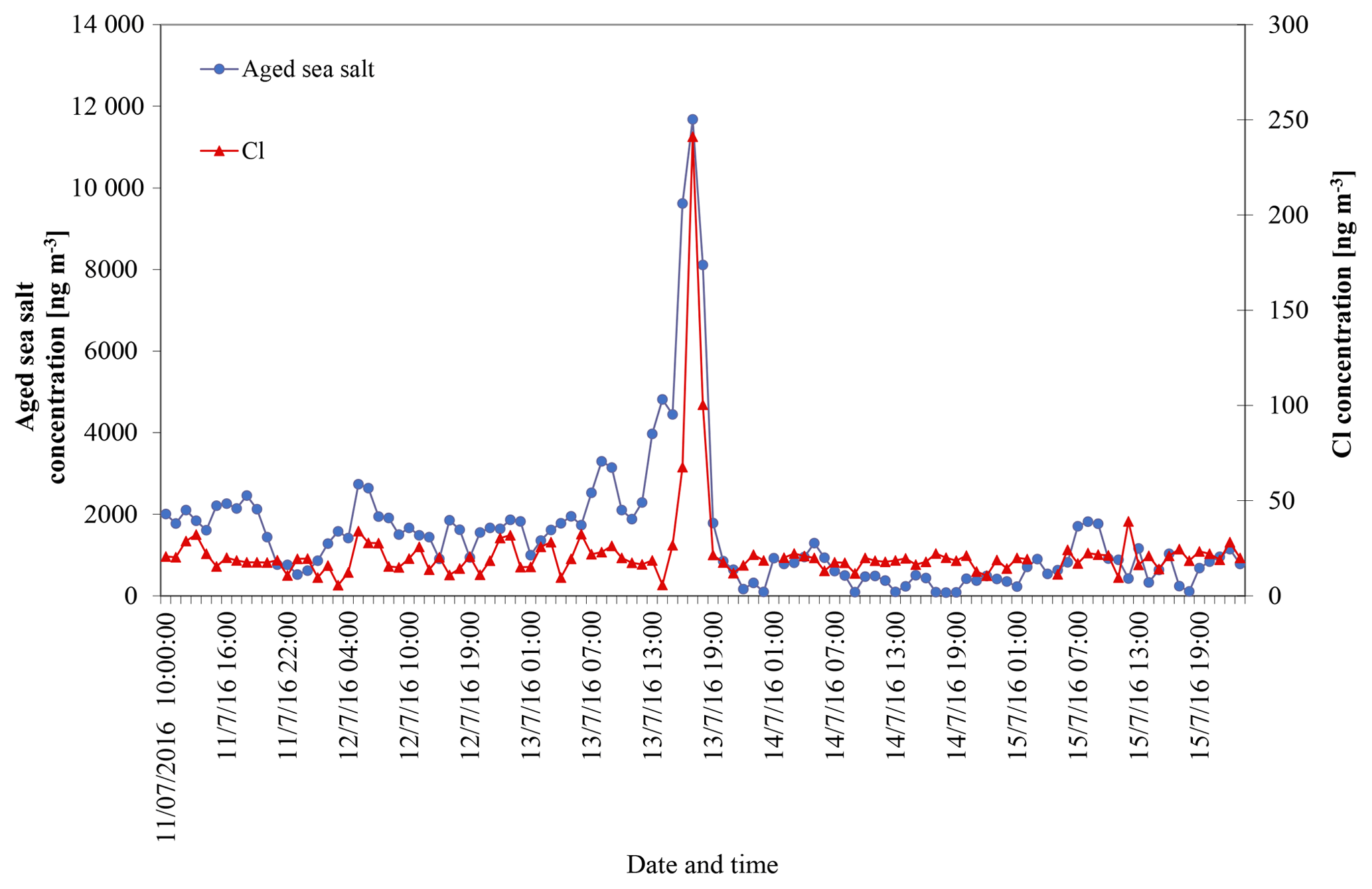
Figure 4 Temporal patterns of an aged sea salt source retrieved from the multi-time resolution model and Cl concentrations measured in atmospheric aerosol.

Bootstrap analysis was performed to evaluate the uncertainties associated with source profiles (Crespi et al., 2016). One-hundred runs were carried out (see Fig. 5, values expressed in ng m⁻³ or Mm⁻¹ on a logarithmic scale); factors were well mapped, with mapping always higher than 97 % considering the Pearson coefficient, and tracers for each source showed a small interquartile range, supporting the goodness of the solution presented in this work.

3.3 Improving source apportionment with optical tracers

First of all, the use of the absorption coefficient determined at different wavelengths as the input variable in the multi-time resolution model strengthened the identification of the sources, suggesting that it can be exploited when specific chemical tracers are not available (e.g. levoglucosan for biomass burning). To prove that, a separate source apportionment study was performed with EPA PMF 5.0 (Norris et al., 2014) using only hourly elemental concentrations from samples collected by the streaker sampler and hourly b_ap at different λ measured by PP_UniMI on the same filters as input variables. Streaker samples typically lack a complete chemical characterization; in particular, important chemical tracers such as levoglucosan and EC are not available. In this analysis, b_ap assessed at different wavelengths was proven effective in identifying the biomass burning factor that explained a significant percentage of the b_ap itself (from 25 % to 35 % depending on λ) (Fig. S5); without the optical variables, the factor-to-source assignment would otherwise be based only on the presence of elemental potassium, although it is well known that K cannot be considered an unambiguous tracer as it is emitted by a variety of sources (see for example Pachon et al., 2013, and references therein). Furthermore, results showed that the absorption coefficient contribution was higher than 45 % in the factor labelled as traffic, highlighting the importance of exhaust emissions in a factor that would be differently characterized by elements related to non-exhaust emissions (Cu, Fe, Cr).

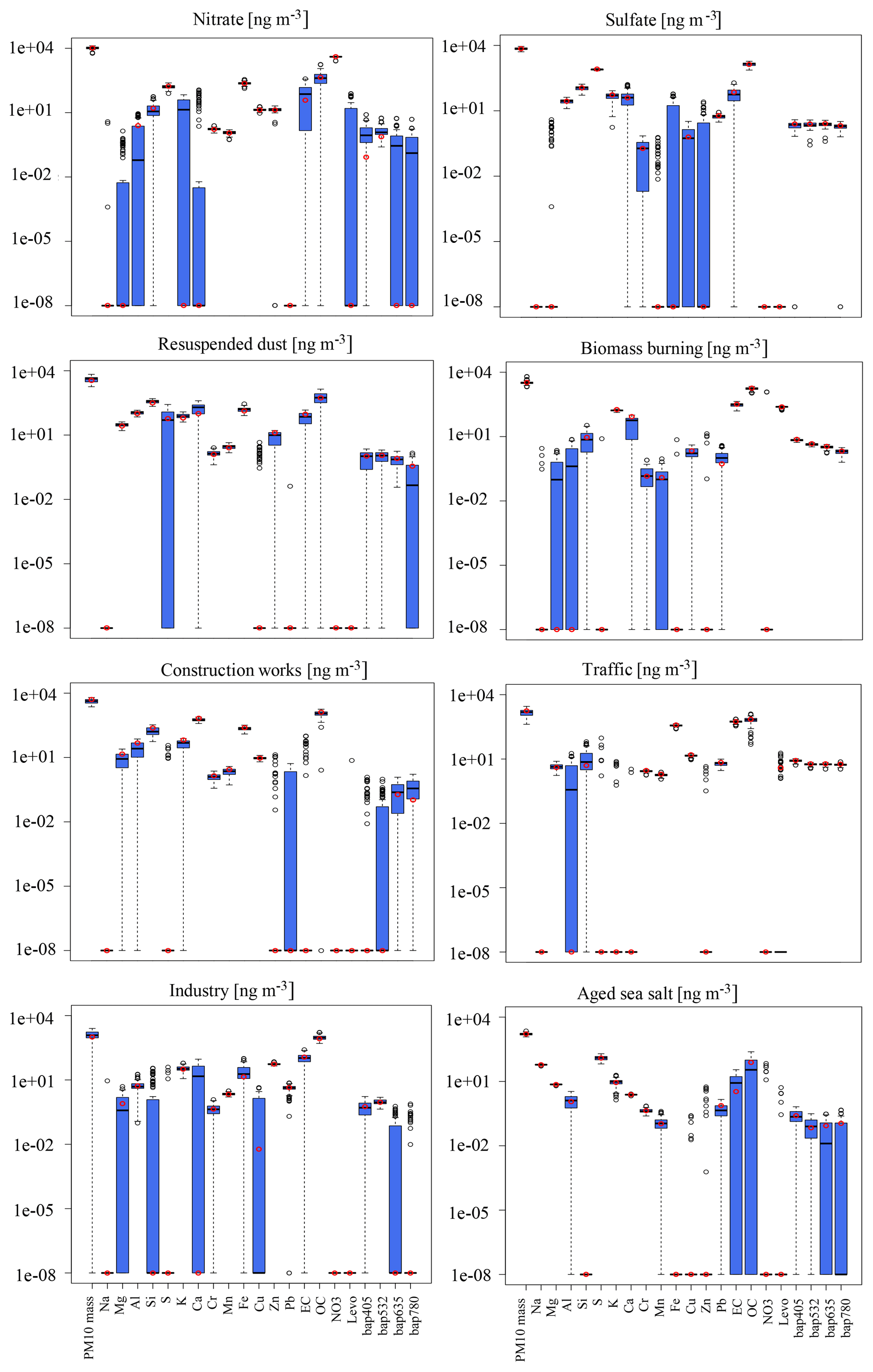
Figure 5 Box plot of the bootstrap analysis on the eight-factor constrained solution. The red dots represent the output values of the solution of the model; the black lines the medians from the bootstrap analysis; the blue bars the 25th and 75th percentiles; the dotted lines the interval equal to 1.5 times the interquartile range; and the black dots the outliers from this interval.

From the multi-time resolution model, the two factors identified as biomass burning and traffic were the main contributors to aerosol absorption in the atmosphere and showed significant EVF values. At 780 and 405 nm, traffic contributions to b_ap were 55 % and 42 %; at the same wavelengths biomass burning accounted for 20 % and 36 %. The EVF of b_ap has the maximum value at 405 nm for biomass burning (0.32) and at 780 nm for traffic (0.49), showing the tendency to decrease and increase with the wavelength, respectively.

The third contributor to aerosol absorption in the atmosphere was the sulfate factor, with a contribution comparable to the biomass burning one at 780 nm (about 20 % of the total reconstructed b_ap at this wavelength). The sulfate factor contained a small fraction of EC, as previously discussed (see Sect. 3.2). This might be explained considering that non/weakly light-absorbing material can form a coating able to enhance particle absorption (Bond and Bergstrom, 2006; Fuller et al., 1999) within a few days after emission. Laboratory experiments and simulations from in situ measurements highlighted absorption amplification for absorbing particles coated with secondary organic aerosol (Schnaiter et al., 2003; Moffet and Prather, 2009). Particle aging is a significant process in the Po Valley due to low atmospheric dispersion conditions and it might explain the relatively high contribution of the sulfate factor to the absorption coefficient in respect to the other sources (apart from traffic and biomass burning). Among the remaining factors, resuspended dust was the main contributor at all wavelengths (between 3 % and 7 % of the total reconstructed b_ap, depending on the wavelength), likely due to the role of iron minerals. The other sources were less relevant in terms of EVF values and overall contributed less than 11 %.

In contrast to the approach used in source apportionment models based on optical data like the widespread Aethalometer model (Sandradewi et al., 2008a) and MWAA model (Massabò et al., 2015; Bernardoni et al., 2017b), it is noteworthy that no a priori information about α values of the fossil fuel and biomass burning sources was introduced in the multi-time resolution model and an estimate for these values was directly retrieved from the model. Another literature approach used Delta-C as an input variable together with chemical aerosol components in source apportionment models and was very effective in separating traffic (especially diesel) emissions from biomass combustion emissions (Wang et al., 2011, 2012).

In order to compare the multi-time resolution model and models based on optical data, contributions due to traffic and industry (i.e. emissions most likely connected to fossil fuel usage) were added up and labelled as “fossil fuel emissions”. In accordance with the two-source approach used in the Aethalometer model, the discussion about optical properties will be hereafter focused on the biomass burning and fossil fuel sources considering that sulfate and resuspended dust factors were less significant also in terms of EVF for optical variables, ranging from 0.08 to 0.12 and from 0.03 to 0.06, respectively, depending on the wavelength.

In Fig. 6 the wavelength dependence of b_ap for the biomass burning and the fossil fuel profiles obtained with the multi-time resolution model is shown; as α values can show significant differences when calculated using different pairs of λ (Sandradewi et al., 2008b), here we performed a fitting procedure considering $b_{\mathrm{ap}}\propto {\mathit{\lambda }}^{-\mathit{\alpha }}$. Results were α_BB (α biomass burning) = 1.83 and α_FF (α fossil fuels) =0.80; the range of variability of α values was estimated with the bootstrap analysis obtaining 0.78–0.88 for α_FF and 1.65–1.88 for α_BB (as the 25th and 75th percentiles, respectively).

Figure 6 b_ap dependence on λ for biomass burning and fossil fuel emissions.

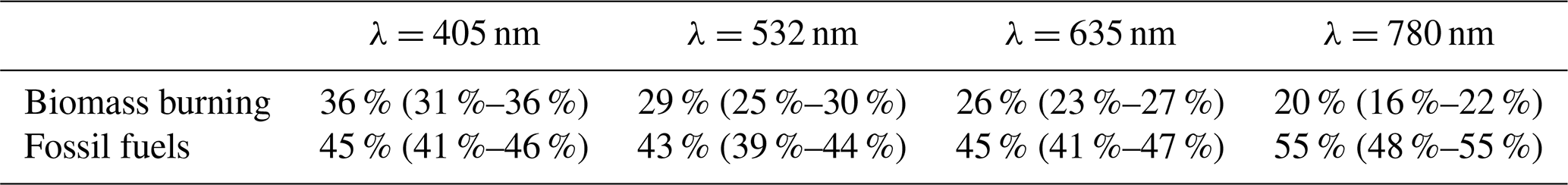
Table 2 Average contribution to total reconstructed b_ap for the biomass burning and fossil fuel factors; in parentheses the 25th and 75th percentiles are reported.

Zotter et al. (2017) reported a possible combination of α_FF=0.8 and α_BB=1.8 when EC concentration from fossil fuel combustion (estimated with radiocarbon measurements) is between 40 % and 85 % of the total EC concentration; in this work, the fraction of EC ascribed by the multi-time model to fossil fuel sources was 56 %. The combination 0.9 and 1.68 for α_FF and α_BB, respectively, was also suggested when in the study there is no or only limited additional information (e.g. from ¹⁴C measurements). From the wide range of possible combinations reported in the literature it is clear that the assessment of α_BC (assumed to be equal to α_FF in source apportionment models based on optical data) is still an issue, and both experimental and simulation studies are in progress to reduce uncertainties and give a better evaluation of this key parameter.

The α_FF value resulted in the range 0.8–1.1 typically reported in source apportionment studies based on optical data (e.g. Bernardoni et al., 2017b; Zotter et al., 2017, and references therein). Indeed, the sampling site was an urban background station in Milan and our samples were hardly impacted by fresh traffic emissions. Considering the aged nature of Milan aerosol, the average α_FF was comparable to estimates for BC-coated particles reported in the literature (approximately 0.6–1.3; see e.g. Liu et al., 2018) and obtained by both ambient measurement (e.g. Fischer and Smith, 2018, and references therein) and numerical simulations (e.g. Gyawali et al., 2009; Liu et al., 2018, and references therein). The α_BB value retrieved by the model was very similar to values reported by Zotter et al. (2017) and also comparable to 1.86 found for biomass burning by Sandradewi et al. (2008a) and 1.8 obtained by Massabò et al. (2015), who also used independent ¹⁴C measurements for checking.

Results here reported also allow us to study the relationship between the absorption coefficient and the mass of black carbon (BC), i.e. the so-called mass absorption cross section, at different wavelengths. The MAC(λ) =b_ap(λ) / BC relationship assumes that BC is the only light-absorbing species present; however, this assumption is not always valid since the transport of mineral dust from desert areas and brown carbon can significantly contribute to aerosol absorption. During our monitoring campaign, no contribution from Saharan dust was observed; in contrast, biomass burning was proven to be an important source, so that BrC was certainly a significant contributor (Fuzzi et al., 2015), as also suggested by α_BB=1.83 in the biomass burning factor. The possible overestimation of BC when total b_ap is ascribed to BC only is usually minimized by choosing a wavelength longer than 600 nm, exploiting the spectral dependence of absorption from different aerosol compounds (Petzold et al., 2013).

EC concentration retrieved from the chemical profiles (see Fig. 3) was used as a proxy for BC to estimate a source-dependent b_ap(λ)-to-BC ratio. Results are represented in Fig. 7. It is noteworthy that here this ratio is intentionally not indicated as MAC, since overestimation of the BC absorption especially at shorter λ might occur (see the previous discussion). BrC is expected to give a small contribution in the fossil fuel source; therefore, the best approximations for MAC(λ) values are likely the b_ap(λ)-to-BC ratios observed in the fossil fuel source at our monitoring site. They resulted in 13.7 m² g⁻¹ for λ=405 nm, 10.2 m² g⁻¹ for λ=532 nm, 8.8 m² g⁻¹ for λ=635 nm, and 8.6 m² g⁻¹ for λ=780 nm. For λ=550 nm, Bond and Bergstrom (2006) reported a MAC value of 7.5±1.2 m² g⁻¹ for uncoated fresh emitted particles and MAC values in polluted regions ranging from 9 to 12 m² g⁻¹, attributable to absorption enhancement due to particle coating. The MAC estimate obtained in this work from the multi-time resolution model for 532 nm is comparable to literature values reported above, thus confirming the importance of aging processes in the atmosphere for the optical properties of particles.

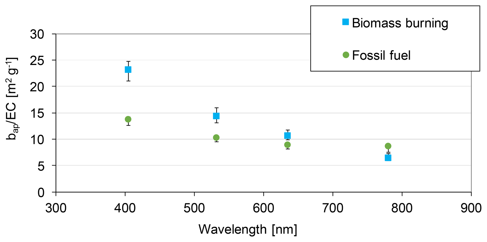
Figure 7 b_ap-to-EC ratio dependence on λ for biomass burning and fossil fuel emissions. Error bars represent the 25th and 75th percentiles retrieved from the bootstrap analysis.

Ratios represented in Fig. 7 are less comparable at λ=405 nm (see also Table S4) due to the significant contribution of BrC to b_ap at this wavelength in the biomass burning factor.

No seasonal differences in the atmospheric ratios were observed except at λ=405 nm (see Table S4), for which winter values were higher than summer ones (17.8±0.4 and 14.2±0.5, respectively), due to the influence of biomass burning emissions on BrC concentration in the atmosphere during the cold season.

From the outputs of the modelling approach here proposed, the apportionment of the biomass burning and fossil fuel contributions to b_ap at different wavelengths was also obtained. As expected, the relative contribution to the total reconstructed b_ap ascribed to the biomass burning factor decreased with increasing λ, in contrast to the contribution from fossil fuel combustion which gave the highest contribution at 780 nm (Table 2); in addition, the latter contribution prevailed at all wavelengths at the investigated site.

4 Conclusions

The multi-time resolution model implemented through the Multilinear Engine (ME-2) script allowed the analysis of experimental data collected at different timescales, coupling the detailed chemical speciation at low time resolution and the temporal information given by high time resolution samples. The use of the aerosol absorption coefficient (b_ap) measured at different wavelengths in the modelling process was investigated and gave promising results. First of all, a more robust identification of sources was provided; secondly, it paved the way to the retrieval of optical apportionment and optical characterization of the sources (e.g. estimate of a source-specific absorption Ångström exponent – α – and a mass absorption cross section – MAC - at different wavelengths). It is worth noting that currently in source apportionment models based on optical data (e.g. Aethalometer model) values for α related to fossil fuel emissions and biomass burning are fixed by the modeller, thus carrying a large part of the uncertainties in the model results. Considering that the estimates for the absorption Ångström exponent were here obtained as a result of a quite complex modelling approach (i.e. using multi-time resolution datasets joining chemical and optical variables) and without any a priori assumption, the results obtained were fairly comparable to literature results and gave a further tool to assess more robust source-related α values. Obviously these estimates are affected by a certain degree of uncertainty due to both experimental data and modelling process (while uncertainties are typically not taken into consideration for fixed α values used in the literature). In perspective, joining together different approaches such as the receptor modelling here proposed and e.g. ¹⁴C data and artefact-free b_ap measurements will lead to better estimates of the absorption Ångström exponent.

The original approach described in this work can be applied to source apportionment studies using any suitable dataset (not necessarily with multi-time resolution). Besides the traditional source apportionment, the impact of different sources on the aerosol absorption coefficient was estimated; this piece of information can be very useful for formulating strategies of pollutant abatement, in order to improve air quality and to face climate challenges. In particular, at the investigated site secondary compounds constituted the highest contribution in terms of PM₁₀ mass (52 % on average), while the two factors identified as biomass burning and traffic were found to be the most significant contributors to aerosol light absorption in the atmosphere, in agreement with the available literature.