the Creative Commons Attribution 3.0 License.
the Creative Commons Attribution 3.0 License.
Detection of critical PM2.5 emission sources and their contributions to a heavy haze episode in Beijing, China, using an adjoint model
Shixian Zhai
Xingqin An
Tianliang Zhao
Zhaobin Sun
Wei Wang
Qing Hou
Zengyuan Guo
Chao Wang
Air pollution sources and their regional transport are important issues for air quality control. The Global–Regional Assimilation and Prediction System coupled with the China Meteorological Administration Unified Atmospheric Chemistry Environment (GRAPES–CUACE) aerosol adjoint model was applied to detect the sensitive primary emission sources of a haze episode in Beijing occurring between 19 and 21 November 2012. The high PM2.5 concentration peaks occurring at 05:00 and 23:00 LT (GMT+8) over Beijing on 21 November 2012 were set as the cost functions for the aerosol adjoint model. The critical emission regions of the first PM2.5 concentration peak were tracked to the west and south of Beijing, with 2 to 3 days of cumulative transport of air pollutants to Beijing. The critical emission regions of the second peak were mainly located to the south of Beijing, where southeasterly moist air transport led to the hygroscopic growth of particles and pollutant convergence in front of the Taihang Mountains during the daytime on 21 November. The temporal variations in the sensitivity coefficients for the two PM2.5 concentration peaks revealed that the response time of the onset of Beijing haze pollution from the local primary emissions is approximately 1–2 h and that from the surrounding primary emissions it is approximately 7–12 h. The upstream Hebei province has the largest impact on the two PM2.5 concentration peaks, and the contribution of emissions from Hebei province to the first PM2.5 concentration peak (43.6 %) is greater than that to the second PM2.5 concentration peak (41.5 %). The second most influential province for the 05:00 LT PM2.5 concentration peak is Beijing (31.2 %), followed by Shanxi (9.8 %), Tianjin (9.8 %), and Shandong (5.7 %). The second most influential province for the 23:00 LT PM2.5 concentration peak is Beijing (35.7 %), followed by Shanxi (8.1 %), Shandong (8.0 %), and Tianjin (6.7 %). The adjoint model results were compared with the forward sensitivity simulations of the Models-3/CMAQ system. The two modeling approaches are highly comparable in their assessments of atmospheric pollution control schemes for critical emission regions, but the adjoint method has higher computational efficiency than the forward sensitivity method. The results also imply that critical regional emission reduction could be more efficient than individual peak emission control for improving regional PM2.5 air quality.
- Article
(4933 KB) - Full-text XML
-
Supplement
(209 KB) - BibTeX
- EndNote


The application of adjoint theory to atmospheric chemistry models can enable the efficient calculation of the sensitivities of a few variables or metrics with respect to a large number of input parameters (Marchuk, 1974; Sandu et al., 2005; Hakami et al., 2007). Classic atmospheric chemistry models use inputs of emission sources to output the spatiotemporal variation of pollutants, which is thus is source oriented. By contrast, adjoint models are receptor-oriented, for they use the gradients of the cost function to model variables (usually pollutant concentrations) as inputs and output the spatiotemporal variations of the sensitivities of the cost function to emissions (Errico, 1997; Carmichael et al., 2008). Therefore, in concentration–source sensitivity analysis, the adjoint method is more computationally efficient than others, such as the traditional finite-difference method, which requires repeated input perturbations and result comparisons (Wang et al., 2015). Moreover, the finite difference approach changes the state of the modeled atmosphere and inevitably incurs truncation and cancellation errors (Constantin and Barrett, 2014). When calculating gradients, the adjoint model integrates under particular atmospheric conditions; thus, it can provide exact sensitivities. Although the adjoint approach is not strictly a method used for source apportionment because it provides merely tangent linear derivatives (gradients) that are likely to be valid over only a limited range of values for the parameters (emissions), it does provide valuable information about the dependence of aerosol concentrations on emissions (Henze et al., 2007, 2009; L. Zhang et al., 2015). If we set the cost function as the pollutant concentration over a region at a point in time (or during a time period), the adjoint sensitivity approach can detect critical emission sources in detail and reveal the changes in concentration due to perturbations in emission sources.
Beijing is a rapidly growing economic center and a densely populated metropolis whose recent PM2.5 pollution problems have garnered considerable attention (Zhang et al., 2016; Sun et al., 2014; Guo et al., 2010; Wu et al., 2015). PM2.5 pollution in Beijing is significantly influenced by the regional transport of pollutants from its environs. As such, the joint control of effective air pollution emission sources has been promoted. Research using approaches such as the flux calculation method (An et al., 2007), the back-trajectory model (Zhai et al., 2016), and observation analysis (Li et al., 2016), have revealed that southerly winds almost always promote high PM2.5 conditions in Beijing. Studies have also indicated that more than 50 % of PM2.5 pollutants originate in surrounding provinces and cities, including southern Hebei, Tianjin, eastern Shanxi, and Shandong provinces (Jiang et al., 2015; Gao et al., 2016). Studies have also shown that joint regional air pollution management control can be more cost-effective (Wu et al., 2015) and that joint control schemes in critical source zones (detected by a back-trajectory model) prior to unfavorable meteorological conditions can help reduce costs and improve efficiency (Zhai et al., 2016). The above studies either determined pollution pathways through meteorological analysis or analyzed air pollutant concentration sensitivities for a limited group of emission sources. If air pollution can be spatially and temporally traced back to its emission sources, decision-making regarding air pollution management can be better addressed.
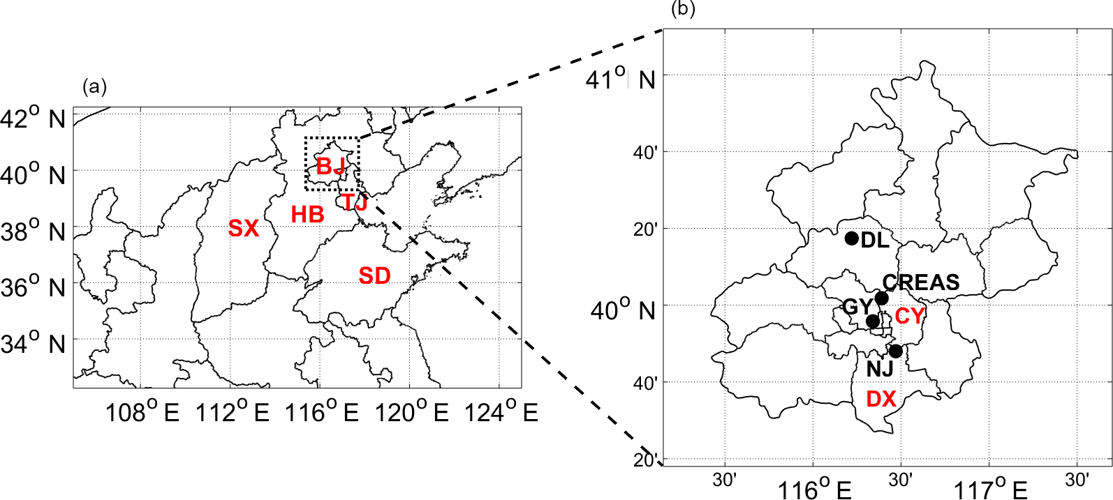
Figure 1(a) Model domain and location of the cities of Beijing (BJ) and Tianjin (TJ) and the provinces of Hebei (HB), Shandong (SD), and Shanxi (SX); (b) locations of the Chinese Research Academy of Environmental Sciences (CRAES), Guanyuan (GY), the Dingling (DL), and Nanjiao (NJ) stations, and the districts of Daxing (DX) and Chaoyang (CY).
Unlike back-trajectory approaches or statistical factor analysis, the adjoint approach accounts for chemical and physical processes combined with transport; thus, it efficiently estimates the incremental influence of specific sources on air quality (Henze et al., 2009). Recently, An et al. (2016) developed the aerosol adjoint module of the atmospheric chemistry modeling system GRAPES–CUACE (the Global–Regional Assimilation and Prediction System coupled with the China Meteorological Administration Unified Atmospheric Chemistry Environment) and estimated the average black carbon (BC) concentrations over Beijing at the highest concentration time with respect to BC amounts emitted over the Beijing–Tianjin–Hebei region. They also indicated the effectiveness of controlling the most influential regions during critical time intervals, as detected by the adjoint sensitivity analysis. Zhang et al. (2015) attributed the sources of Beijing's PM2.5 by using the GEOS-Chem adjoint model and summarized that residential (49.8 %) and industrial sources (26.5 %) are the largest contributors. They further noted that 45–53 % of PM2.5 pollutants in Beijing and Tianjin are from local sources, whereas the Hebei province sources contribute approximately 26 %. Both Zhang et al. (2015) and An et al. (2016) demonstrated the high efficiency and accuracy of the atmospheric chemistry adjoint model in identifying Beijing air pollution sources.
In this study, we apply the newly developed GRAPES–CUACE aerosol adjoint model (An et al., 2016) to track the sensitive primary emission sources of a high PM2.5 episode that occurred in Beijing in November 2012. The two PM2.5 concentration peaks that occurred were set as the cost functions. By detecting the primary emission sources of these two hourly PM2.5 peaks, our work advances the understanding of the impacts of emission sources by providing detailed insights into the spatial and temporal variability of emission source contributions from each of the surrounding provinces and from local and environs transports. We then set the average PM2.5 concentration from 21 November as the cost function and compared the adjoint model results with the Models-3/CMAQ assessments (Zhai et al., 2016). Furthermore, we also compared emission source impacts on the Beijing PM2.5 concentration peak from zones with maximum adjoint sensitivities and emission-intensive zones. This study explores the capability of the GRAPES–CUACE aerosol adjoint model to simulate detailed concentration–source relationships and provide guidance for flexible environmental control policy.
Atmospheric stability and humidity over the mid-eastern region of China from 19 to 22 November 2012 were analyzed in combination with the results of the Meteorological Information Comprehensive Analysis Processing System, the sounding stratification and dew point–pressure curves (temperature–logarithmic pressure diagrams) from Nanjiao station (Fig. 1a) in Beijing (Fig. 2), and the flow field pattern. Meanwhile, the formation of two pollution peaks at dawn and at night on 21 November 2012, was also qualitatively analyzed. During the period between 19 and 20 November, Beijing was under the influence of a low-pressure system situated between two high pressures. During the daytime, southerly winds prevailed below 925 and 1000 hPa, and the relative humidity increased during this time period. During the nighttime, southerly winds shifted to northeasterly and easterly winds, thus transporting pollutants, together with water vapor, to Beijing. In this same time period, thermal inversions occurred below 850 hPa. The above analysis reveals that the accumulation of PM2.5 concentrations was tightly connected with southerly winds during the daytime and easterly winds at night.
During the daytime on 21 November, the Beijing–Tianjin–Hebei area was located at the bottom of a high-pressure system, with easterly winds prevailing in the 850 hPa layer. The thermal inversion remained, and the relative humidity continued to increase. The south-central part of Hebei province was influenced by a mass of cold air controlled by northerly winds, whereas Beijing was mainly under the influence of an easterly wind that promoted pollutant convergence in front of the Taihang Mountains and carried abundant water vapor, which accelerated the hygroscopic growth of local particles. It can be concluded that the pollution peak on the night of 21 November was not only the result of the accumulation of pollutants during the previous 2 days but also the result of the hygroscopic growth of local particles and the convergence of pollutants caused by daytime easterly winds. According to prior research (Chen et al., 2016; Li et al., 2016), this event was typical of a synoptic episode that gradually generates air pollution over Beijing until a sudden and significant improvement in air quality due to strong winds. This is also the same episode that was analyzed by Zhai et al. (2016), thus facilitating further comparisons.
3.1 Concepts of the adjoint sensitivity analysis
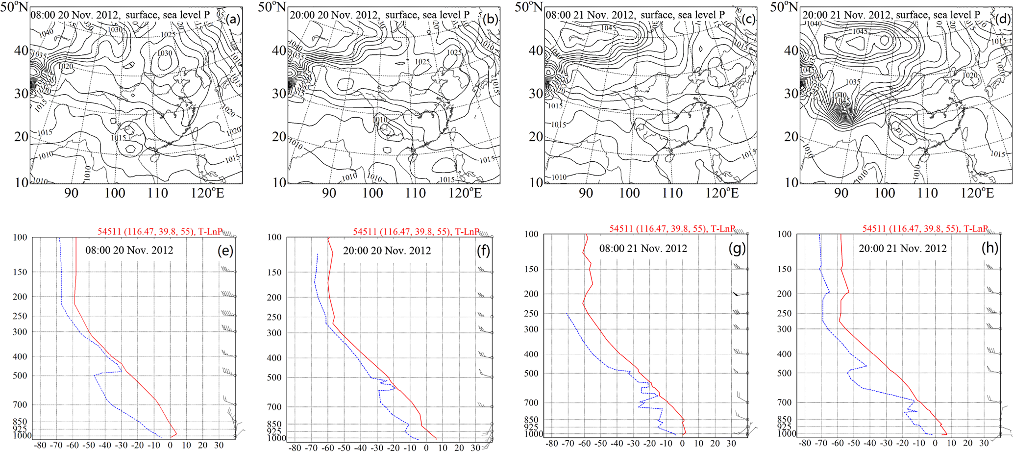
Figure 2(a–d) Sea-level pressure field; (e–h) temperature–logarithmic pressure diagrams (blue dotted curves indicate dew point–pressure; red solid curves indicate stratification) at the Nanjiao station from 08:00 LT 20 November 2012 to 20:00 LT 21 November 2012.
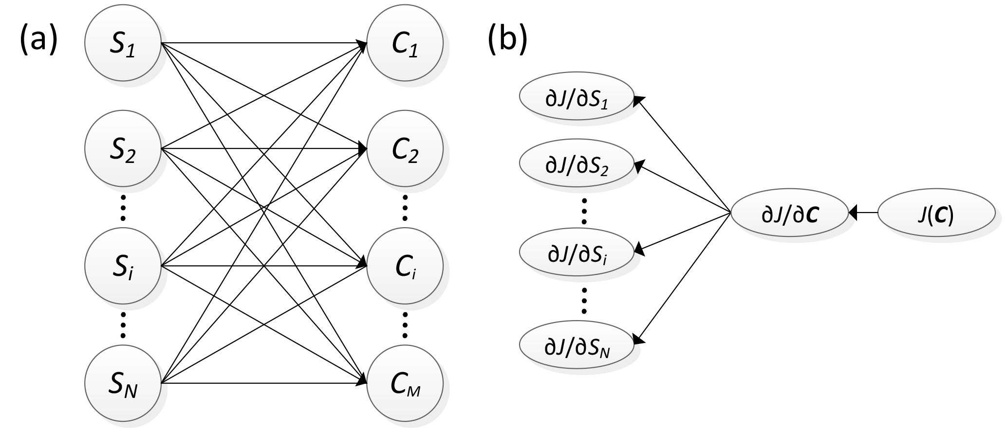
Figure 3Schematic diagrams of the atmospheric chemistry forward (a) and adjoint (b) models. are emission sources of different sectors, or of different species, at different locations, etc., and S is the emission vector; are pollutant concentrations at different sites, or of different species, and C is the concentration vector.
Sensitivity analysis plays an important role in atmospheric environmental research. Understanding the impacts of emissions on pollutant concentrations is helpful for the development of effective air pollution control strategies. The adjoint model is efficient in calculating the sensitivity of a cost function to any model variable at any time step. Figure 3 shows the schematic diagrams of the forward atmospheric chemistry model and the adjoint model. The atmospheric chemistry model takes emissions (S: S1, ) as inputs and outputs pollutant concentrations (C: through forward integration. Any emission source (Sn) might have an influence on the concentration at any receptor site (Cm). A pair of emission source sensitivity tests using the traditional source-oriented finite-difference method can determine the contribution of an emission source (or a combined group of emission sources) to the pollution level at any receptor site. Therefore, with N emission sources and M receptors in total, the contribution from each of the N emission sources to each of the M receptors (an N×M matrix) can be obtained through N+1 iterations of forward integration (one base simulation included). The receptor-oriented adjoint model is complementary to the forward model. The sensitivity map of a scalar function of pollutant concentration (the cost function) to every emission source (N×1 matrix) can be obtained by performing one backward adjoint integration (Sandu, 2005; An et al., 2016; Zhai, 2015), with the above-mentioned N×M matrix requiring M iterations of the adjoint integration. Theoretically, the N×M matrices resulting from the forward and backward methods are the same within a small perturbation (Marchuk, 1986), considering the nonlinearity of PM2.5 formation.
Adjoint sensitivities are the tangent linear derivatives (gradients) of the cost function to model parameters (emissions) and are likely to be valid over only a limited range of values for each parameter (Henze et al., 2007, 2009). In this study, the GRAPES–CUACE aerosol adjoint model considered only primary PM2.5 (explained in Sect. 3.2), and the primary PM2.5 emission sources and PM2.5 concentrations had an approximately linear relationship (see Fig. S1 in the Supplement). Given the linear relationship between the concentration of PM2.5 and its primary emission sources, the magnitude of perturbations did not influence the representative of the adjoint sensitivities when comparing the contributing proportions of emission sources from different regions. However, if the adjoint sensitivities are used to represent the absolute emission source contributions, errors will increase with an increase in perturbations. In Fig. S1, we can see that the adjoint sensitivity results are similar to the finite difference results, and the difference between the adjoint sensitivity results and the finite difference results grows with the increase of emission reduction ratios (the blue line with circular symbols and the red line with triangle symbols are close, particularly when the x axes are within 30 %); therefore, the adjoint sensitivity coefficients are likely to be representative over PM2.5 primary emission reduction ratios from 5 to 90 % or at least over a modest range of emission perturbations commensurate with typical emission abatement strategies (10–30 %). All in all, an atmospheric chemistry model is suitable for simulating air pollution processes, whereas an adjoint model is efficient in quantifying receptor–source relationships.
The adjoint model can calculate the sensitivity of the cost function (J) to any emission source (Sn), as denoted by . If we compare a group of uniformly distributed emission sources, larger values indicate the greater influence of Sn on J. However, emission intensities are obviously not uniform across urban and rural areas, and seasonal and diurnal changes add even more nonuniformity. Furthermore, the emissions of different species of pollutants may have different units and may differ in their order of magnitude. Under these circumstances, the relative contribution of each emission source cannot be determined only by calculating the gradient . Therefore, we define the sensitivity coefficients in this study as (, which shares the same unit as the cost function and reflects the absolute changes in the cost function due to perturbations in emission sources; this definition makes the contrast between emission sources more convenient.
3.2 Model description
The GRAPES–CUACE is an online coupled atmospheric chemistry modeling system (Wang et al., 2009; Zhou et al., 2012; Jiang et al., 2015) developed by the China Meteorological Administration (CMA). GRAPES-Meso is a regional meteorological model (Xue et al., 2008) within GRAPES–CUACE, and CUACE is an atmospheric chemistry modeling system independent of meteorological and climate models. The CUACE system adopted the Canadian Aerosol Module (CAM; Gong et al., 2003), a size-segregated multi-component aerosol algorithm, as its aerosol module and the second-generation Regional Acid Deposition Model (RADM II; Stockwell et al., 1990) as its gaseous chemistry model. CAM contains computations for numerous major aerosol processes in the atmosphere: generation, hygroscopic growth, coagulation, nucleation, condensation, dry deposition/sedimentation, below-cloud scavenging, aerosol activation, and chemical transformation of sulfur species in clear air and in clouds (Gong et al., 2003), which is coherently integrated with the gaseous chemistry component in CUACE. Given that the nitrates and ammonium formed through gaseous oxidation are unstable and prone to further decomposition back to their precursors, CUACE adopts ISORROPIA to calculate the thermodynamic equilibrium between them and their gas precursors (Zhou et al., 2012). The CUACE system is compatible with various kinds of meteorological models and can be used as a common platform for atmospheric constituent calculation.
The GRAPES–CUACE aerosol adjoint model was developed by applying adjoint theory to the GRAPES–CUACE modeling system. The current version of the adjoint model includes the adjoint of CAM (Gong et al., 2003), the adjoint of the three interface programs that pass meteorological variable values from GRAPES-Meso to chemical processes in CUACE, and the adjoint of the aerosol transport processes. Considering that the adjoint of the gaseous chemistry (RADM II) and the adjoint of the thermodynamic equilibrium (ISORROPIA) processes are not included in the GRAPES–CUACE aerosol adjoint model, the GRAPES–CUACE aerosol adjoint model is capable of simulating sensitivities of the cost function to primary PM2.5 sources. Hence Sn defined in Sect. 3.1 refers to primary PM2.5 sources. After the tangent linear model (TLM) and the adjoint model are built (the adjoint model is a concomitant of the TLM), they are divided into smaller sections and tested separately before the assembled TLM and the adjoint model are confirmed valid. The details of the adjoint verification can be found in An et al. (2016).
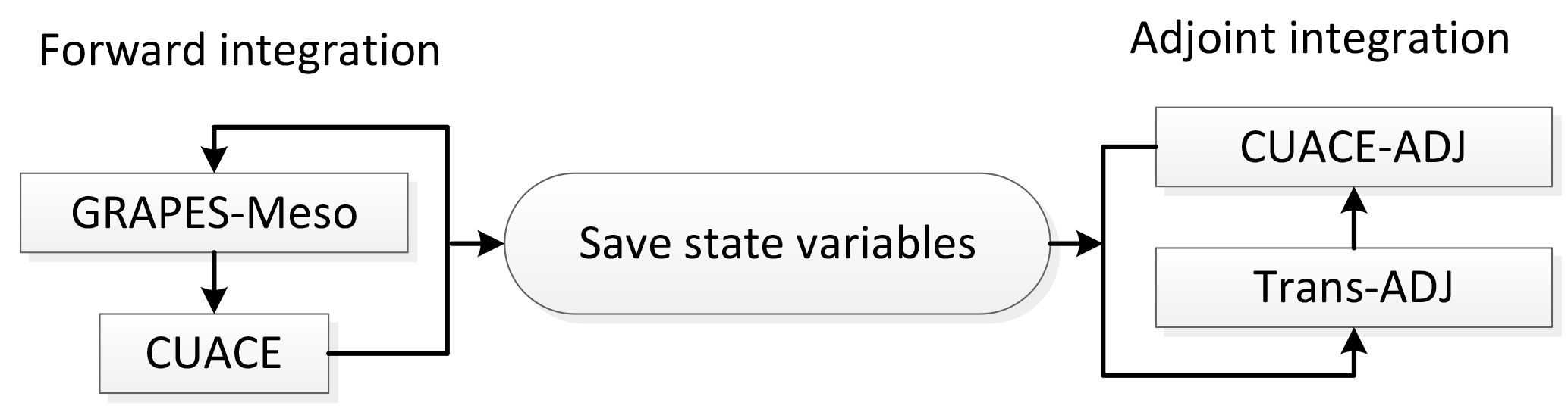
Figure 4 shows the operational processes used in this study. To ensure that the forward and backward models were in the same chemical state, the forward GRAPES–CUACE model was first integrated to save the model state variables (concentrations) in checkpoint files at the beginning of each external time step (Sandu et al., 2005; Henze et al., 2007). These saved variables were then inputted at each checkpoint during the backward adjoint integration. To handle intermediate variables, this study adopted both recalculation and stack storage (PUSH and POP) schemes. Details about the construction, framework, and operational flowchart of the GRAPES–CUACE aerosol adjoint model are discussed in An et al. (2016).
3.3 Model setup, data, and validation
The simulated domain in this study covered northeast China (105–125∘ E, 32.25–42.25∘ N; Fig. 1), which included 41×23 simulation grid cells with 31 vertical layers at the resolution of 0.5∘ × 0.5∘. The model was integrated at a time step of 300 s. The National Centers for Environmental Prediction Final Analysis dataset was used to define the initial meteorological field and the meteorological boundary conditions. The initial and boundary values for O3 and OH were taken from climatic means and zeros for each aerosol species during the first run; thereafter, the daily initial values of all chemical species were determined by the 24 h forecast made by the previous day's simulation. To eliminate the discrepancy between the idealized initial concentration field and the real concentration field, the simulation was started at 20:00 Beijing LT (GMT+8) on 10 November 2012, with the analysis period running from 20:00 LT on 17 November 2012, to 19:00 LT on 22 November2012.
This study used hourly gridded off-line emission sources processed by the SMOKE module, which is based on statistical data of anthropogenic emissions reported from government agencies for 2007. Anthropogenic emissions include primary PM2.5 and pollutant gases (Cao et al., 2011). Emission source types included biomass combustion, residences, power generation, industry, transportation, livestock and poultry breeding, fertilizer use, waste disposal, solvent use, and light industrial product manufacturing (Cao et al., 2011). Furthermore, natural sea salt and natural sand/dust emissions were also calculated in the model.
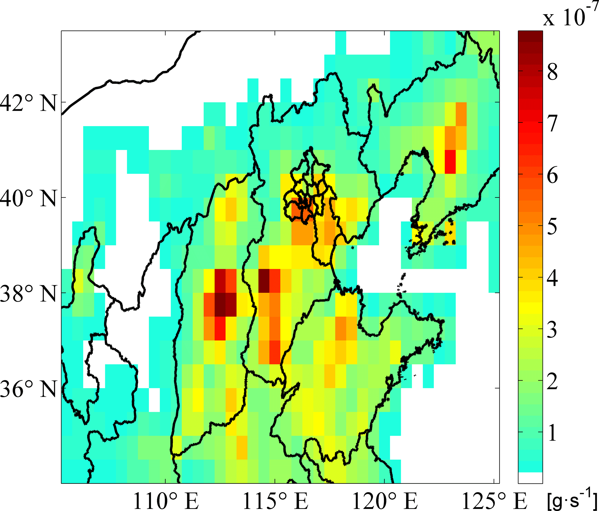
Figure 5 illustrates the gridded distribution of the overall primary PM2.5 sources. Figure 6 shows the hourly variability of the overall PM2.5 sources in Beijing. In Fig. 5, there are four intensive source zones over Beijing and its surrounding provinces: (1) southern Beijing and Tianjin (TJ), (2) southern Hebei (HB), (3) middle Shanxi (SX), and (4) north central Shandong (SD). Meanwhile, a secondary intensive source zone was observed over northern SX. In Fig. 6, it is noted that the overall primary PM2.5 source emission intensity decreased to its lowest level at 05:00 LT. Thereafter, emission intensity began to increase and remained high from 11:00 to 19:00 LT, with a minimum at 14:00 LT.
The observation data includes meteorological elements (2 m temperature and 10 m wind speed) and PM2.5 concentrations. The meteorological data were collected from the Nanjiao (NJ: 116.47∘ E, 39.8∘ N), Haidian (HD: 116.28∘ E, 39.93∘ N), and Shangdianzi (SDZ: 117.12∘ E, 40.65∘ N) stations. The NJ and HD stations are representative urban observatory stations and the SDZ station is a typical background station. These three stations are part of the measurement network run by the Beijing Meteorology Bureau and use standard measurement equipment and methods. PM2.5 measurements used in this study were obtained from the observation stations of the Chinese Research Academy of Environmental Sciences (CRAES: 116.39∘ E, 40.03∘ N), as well as of Guanyuan (GY: 116.34∘ E, 39.93∘ N) and Dingling (DL: 116.22∘ E, 40.29∘ N). The CRAES station is located in the northwest Chaoyang district at the Chinese Academy of Environmental Sciences, and the GY station is located in Xicheng district. Both the CRAES station and the GY station are representative urban observation stations in Beijing. The DL station is located in the relatively clean Changping district in northern Beijing and provides background values for observed PM2.5 concentrations (Fig. 1).

The reliability of the GRAPES–CUACE modeling system is evaluated in terms of both meteorological and chemical simulations. Figure 7 shows the hourly variations of the observed and simulated 2 m temperature (T2 m) and 10 m wind speed (WS10 m), and Table 1 lists the corresponding statistical parameters. The correlation coefficients (R values) between the observed and simulated hourly T2m are 0.77, 0.75, and 0.74, passing the 99 % confidence level with root mean square error (RMSE) values of 1.5, 1.6, and 1.7 ∘C, respectively, at observatory sites NJ, HD, and SDZ. Mean bias (MB) values for the T2m demonstrate a slight underestimation in NJ (−0.1 ∘C) and HD (−0.3 ∘C), and overestimation in SDZ (0.8 ∘C). The variations of the WS10m are generally captured by the model with R values of 0.70, 0.73, and 0.46, and with RMSEs of 1.4, 1.5, and 1.8 m s−1 at NJ, HD, and SDZ stations, respectively (passed the 99 % confidence level). Overall, the GRAPES-Meso could reasonably reproduce the observed meteorology.
Table 1Performance statistics between observed and simulated meteorology.
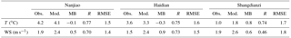

Figure 7The temporal variations of observed and simulated hourly 2 m temperature (T2m) (a–c) and 10 m wind speed (WS10m) (d–f) at Nanjiao, Haidian, and Shangdianzi stations. The observed WS10m are 10 min averaged wind speed for 17–23 November 2012.

Figure 8(a–c) Comparisons of the observed (black solid triangles) and simulated (blue dotted line) hourly PM2.5 concentrations at the CRAES, GY, and DL stations; (d) hourly variations in the average PM2.5 concentrations over Beijing. Please note that the date and time are given in DD HH:MM format, with all dates in November 2012.
Figure 8a–c shows the observed and simulated hourly PM2.5 concentration curves from 20:00 LT on 17 November to 19:00 LT on 22 November at the CRAES, GY, and DL observational stations, and Table 2 lists the statistical parameters. Figure 8a–c reveal that the results of the GRAPES–CUACE modeling system correspond well with the synoptic analysis of the pollution episode. The modeling system was able to reproduce the PM2.5 accumulation processes observed from 19 to 21 November in Beijing and captured the two PM2.5 hourly concentration peaks during the dawn and night of 21 November, as well as the minimum during the afternoon on 21 November at the CRAES, GY, and DL stations, with correlation coefficients (R values) of 0.87, 0.91, and 0.69, respectively (Table 2). However, the model overestimated PM2.5 concentration values over the period with normalized mean biases (NMBs) of 57.2, 108.1, and 10.7 % at the CRAES, GY, and DL stations, respectively. The overestimation was also reflected in the positive mean bias (MB) and mean fractional bias (MFB) values. For the CRAES, GY, and DL stations, the MFBs were 53.6, 65.2, and 15.6 %, respectively, and the corresponding mean fractional errors (MFEs) were 60.1, 68.3, and 39.6 %, respectively. MFEs and MFBs are all within the criteria proposed by Boylan and Russel (2006) – model performance criteria are met when the MFE and MFB are less than or equal to approximately +75 and ±60 %, respectively, except for the MFB at GY, which is a little high. Secondary aerosol formations are important processes in atmospheric physics and chemistry and have large uncertainties, according to the current understanding of the atmospheric environment. The lack of heterogeneous chemical reactions (Wang et al., 2016; Cheng et al., 2016; Guo et al., 2014; Zhang et al., 2015) in the forward GRAPES–CUACE model could be a factor contributing to the modeling uncertainties in this study. Generally, the three factors controlling the discrepancies in air quality modeling are as follows: (1) air pollutant emissions, (2) physical and chemical processes in the atmosphere, and (3) meteorology, particularly in the boundary layer (An et al., 2013; Cheng et al., 2016; Wang et al., 2015a, 2016). The overestimation of PM2.5 in this study might be attributed to the uncertainties of these three factors in the model. Prior studies (Zhou et al., 2012; Wang et al., 2015a, b; Jiang et al., 2015) have demonstrated the stable simulation performance of the GRAPES–CUACE modeling system in reproducing air pollution levels and variation trends over northeast China. Above all, the following analysis mainly focuses on the variations and the contributing proportions of emission sources over different regions. Therefore, adjoint sensitivity analysis was not significantly affected by the overestimation of PM2.5, and these modeling results can be considered reliable.
Table 2Performance statistics of PM2.5 concentrations.
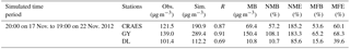
Note that mean bias: ; normalized mean bias: ; normalized mean error: ; mean fractional bias: MFB ; mean fractional error: MFE .
4.1 Simulated haze episode and cost function
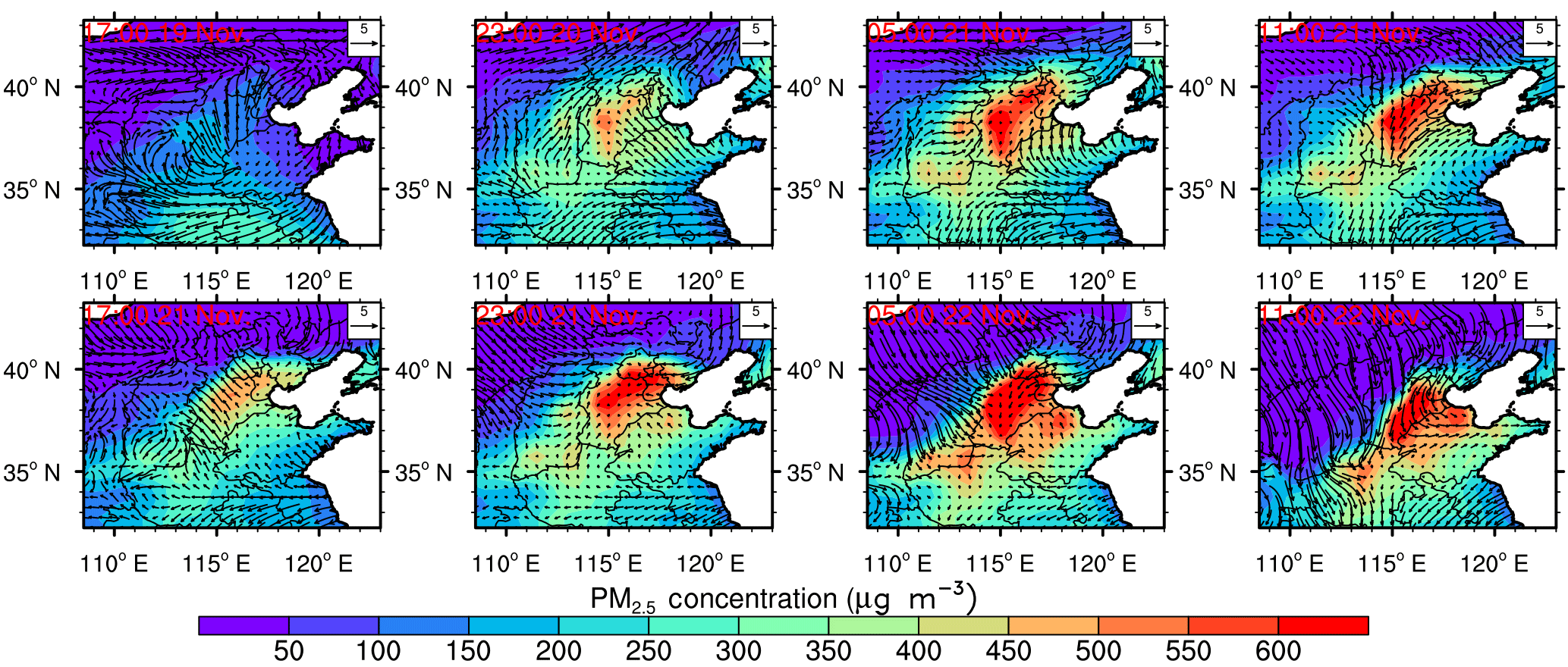
Figure 9 shows the simulated surface PM2.5 concentrations and the wind field variations from 17:00 LT on 19 November to 11:00 LT on 22 November. It can be seen that the simulation results are consistent with the qualitative weather analysis of this time period. From 19 to 20 November, PM2.5 accumulated in Beijing under the influence of a convergent wind field pattern: a southerly wind field to the south, an easterly wind field to the east, and a westerly wind field to the west. From 05:00 to 11:00 LT on 21 November, PM2.5 concentrations exceeded 550 µg m−3 over southern Beijing, south-central Hebei, and northwest Tianjin. After this peak, PM2.5 concentrations over Beijing, south-central Hebei, and Tianjin decreased to a minimum in the afternoon, before rising again to above 550 µg m−3 at 23:00 LT. The decrease in PM2.5 concentrations from the morning to the afternoon is typical for Beijing and resulted mainly from diurnal variation of the planetary boundary layer, with vertical mixing after sunrise effectively diluting the pollutants (Zhao et al., 2009; Liu et al., 2015; Tang et al., 2016). The concentration peak at 23:00 LT was driven by the influence of the easterly winds, which caused pollutant convergence against the Taihang Mountains and carried abundant water vapor that promoted local hygroscopic growth. Thereafter, during the daytime on 22 November, a notable northwesterly wind dispersed pollutants in Beijing, thus ending this pollution episode.
The municipality of Beijing (covering both rural and urban Beijing) experienced two hourly PM2.5 concentration peaks at 05:00 and 23:00 LT on 21 November (Fig. 8d), similar to those observed at the three observation stations. These peaks resulted in the observed high daily average PM2.5 concentration on 21 November, which was analyzed in previous research (Zhai et al., 2016). To analyze the critical emission sources of the two hourly PM2.5 concentration peaks, we took advantage of the adjoint model for simulating concentration–emission relationships and defined two cost functions as the hourly mean PM2.5 concentrations over Beijing at (i) 05:00 LT and (ii) 23:00 LT on 21 November. To demonstrate the reliability and efficiency of the GRAPES–CUACE aerosol adjoint model to provide guidance toward effective and flexible air quality control designs, a third cost function was defined as (iii) the average PM2.5 concentration over Beijing on 21 November. Subsequently, comparisons between results from the GRAPES–CUACE aerosol adjoint model and the Models-3/CMAQ assessments (Zhai et al., 2016) were made.
4.2 Spatial distribution of primary PM2.5 emission source sensitivity coefficients
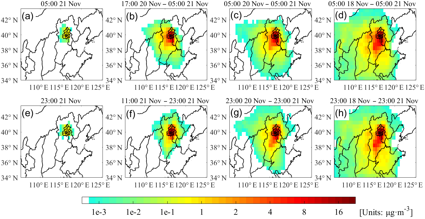
Figure 10Time-integrated sensitivity coefficients of surface Beijing PM2.5 concentration peaks to primary PM2.5 sources. (a–d) 1, 12, 24, and 72 h integrated sensitivity coefficients for the 05:00 LT PM2.5 concentration peak on 21 November; (e–h) 1, 12, 24, and 72 h integrated sensitivity coefficients for the 23:00 LT PM2.5 concentration peak on 21 November.
Figure 10 illustrates the distribution of time-integrated sensitivity coefficients to emission sources for the two concentration peaks in the hourly PM2.5 in Beijing. The sensitivity coefficients of the cost function to emission sources connected pollutants with emissions and revealed the incremental impacts of emissions on peak PM2.5 concentrations. A larger sensitivity coefficient value corresponds to its greater influence on the cost function, J. For example, the largest sensitivity coefficient in Fig. 10d was in the cell that includes Daxing district, with a value of 22.4 µg m−3. This indicates that emissions stemming from this area had the greatest influence on the peak concentration when integrated over 72 h. If emissions were reduced within a small range, the decrease in PM2.5 concentrations should be linear. For example, if emissions from this cell were reduced by N % from 05:00 LT on 18 November to 05:00 LT on 21 November, the target PM2.5 concentration would decrease by N % ⋅ 22.4 µg m−3.
When looking at the accumulation along an inverse time sequence, as shown in Fig. 10a–h, the more influential regions (regions with relatively larger sensitivity coefficients) extended from local Beijing (the target region that covers the entire municipality) to its surrounding provinces. This phenomenon reflected that the PM2.5 pollution episode in Beijing was not only the result of local emissions but also the result of emissions from surrounding regions, including Hebei province, Tianjin, and even Shanxi and Shandong provinces. Emissions from the surrounding areas were continuously transported to Beijing 2 to 3 days ahead of the peak pollution day, thus leading to the observed increase in Beijing's air pollution concentration.
There are differences in the variations in the more sensitive emission regions of these two PM2.5 concentration peaks. First, by comparing the 12 h cumulative sensitivity coefficient distributions in Fig. 10b and f, we can see that emissions to the southwest of Beijing already had a clear influence on the 05:00 LT, 21 November PM2.5 concentration peak (Fig. 10b). However, for the 23:00 LT, 21 November PM2.5 concentration peak, the influential emission sources were still concentrated over Beijing (Fig. 10f), with only a small fraction of influential emissions coming from the east and south of Beijing. This is due to the southwesterly airstream positioned to the southwest of Beijing from 23:00 LT on 20 November to 05:00 LT on 21 November, and the southeasterly water vapor imported during the afternoon and night of 21 November, which caused the moisture–absorption growth of local particles and brought pollutants from Tianjin.
Second, it can be seen from the distributions of the 24 (Fig. 10c and g) and 72 h (Fig. 10d and h) cumulative sensitivity coefficients that sensitivity coefficients both in and around Beijing had relatively large values, thus indicating that both of these PM2.5 concentration peaks were influenced by local and surrounding emissions. However, the most influential emission regions differed between the two PM2.5 concentration peaks. For the first PM2.5 concentration peak, the key 24 h source regions (Fig. 10c) were distributed over Beijing and to the west and south of Beijing. The key 72 h source regions (Fig. 10d) were to the northeast in Shanxi province. However, for the second PM2.5 concentration peak, the key 24 h source regions were mainly located to the south of Beijing (Fig. 10g), whereas the key 72 h source regions were to the west of Beijing (Shanxi province; Fig. 10h) and covered a smaller area than that for the first PM2.5 concentration peak (Fig. 10d).
The results of these simulations show that the variation in the distribution of the sensitivity coefficients, the meteorological conditions, and the pollution evolution processes correspond with each other very well. This indicates that the GRAPES–CUACE aerosol adjoint model is capable of estimating the sensitivity of concentrations to emission sources by propagating a perturbation in concentration backward in time by incorporating meteorological and chemical processes.
4.3 Influence of local and surrounding emission sources on peak PM2.5 concentrations
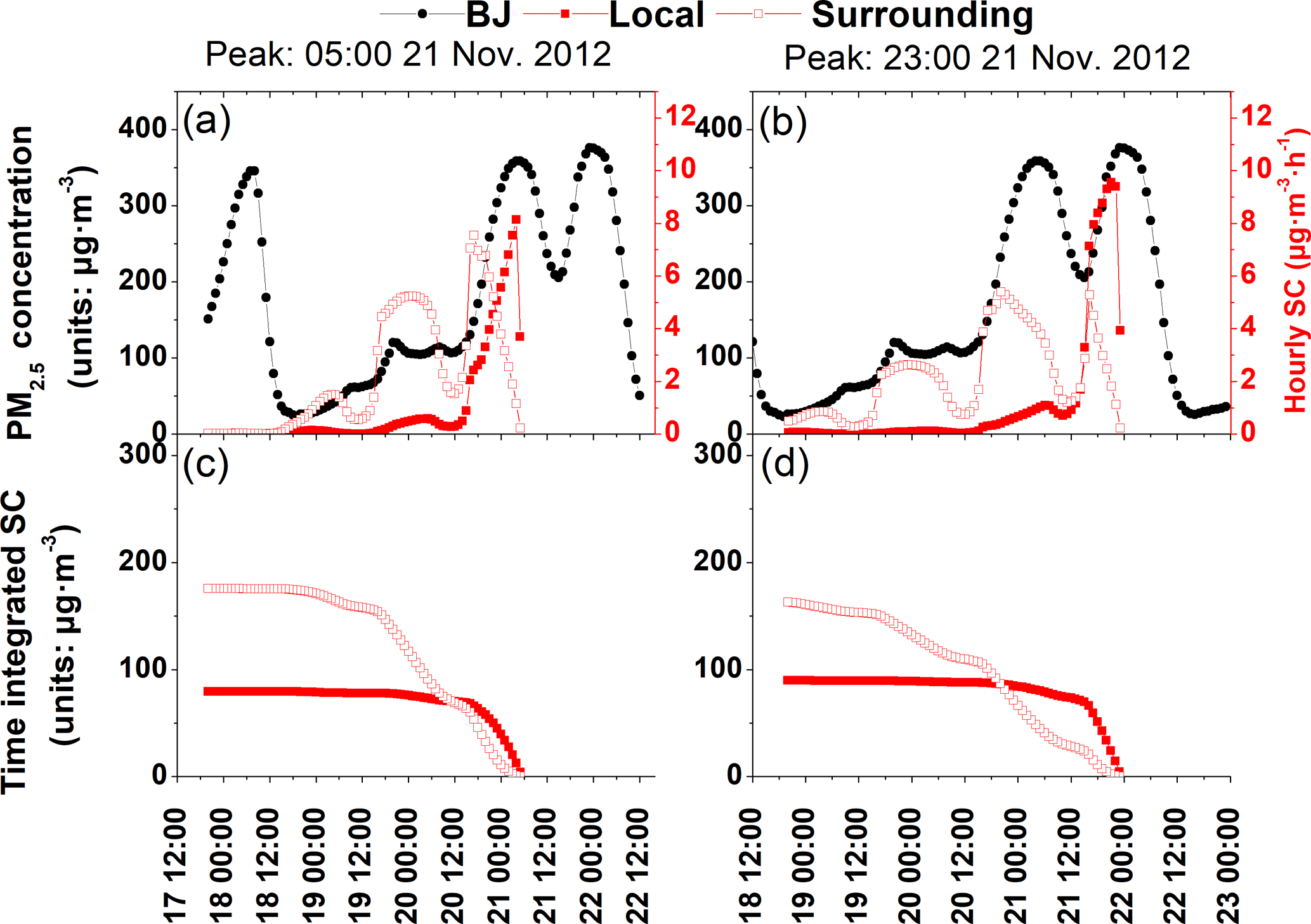
Figure 11Hourly variations of surface PM2.5 concentrations in Beijing and sensitivity coefficients of surface PM2.5 concentration peaks in Beijing to local and surrounding primary PM2.5 sources. The left and right panels correspond to PM2.5 concentration peaks at 05:00 and at 23:00 LT on 21 November 2012, respectively. (a–b) Hourly variations of Beijing PM2.5 concentrations (black solid dotted line) and hourly instantaneous sensitivity coefficients to local (solid red squares) and surrounding (red open squares) emission sources. (c–d) The time-integrated sensitivity coefficients to local (solid red squares) and surrounding (red open squares) emission sources. Please note that the date and time are given in DD HH:MM format, with all dates in November 2012.
Figure 11 illustrates the hourly instantaneous sensitivity coefficients to local Beijing (the target region that covers the entire municipality), its surrounding emission sources (emissions from Hebei, the city of Tianjin, and Shandong and Shanxi provinces; Fig. 11a and b), and their corresponding time-integrated series (Fig. 11c and d). The magnitudes of the sensitivity coefficients reflect the incremental influence of local and surrounding emissions to the objective PM2.5 peaks. It can be seen that the instantaneous sensitivity coefficients of the PM2.5 concentration peaks to local (solid red squares) and surrounding (red open squares) emissions increased to their maximal points before showing a decreasing tendency. However, detailed comparisons of the hourly contribution revealed significant differences between the local and surrounding emissions.
When studying Fig. 11a and b along a reversed time sequence, the local emission sensitivity coefficient maximums (solid red squares) and the PM2.5 concentration peaks (solid black circles) appeared at almost the same time, with the latter delayed by 1 to 2 h. This indicates that local emissions released 1 to 2 h ahead of the PM2.5 peak values were the main contributors to the peak pollution concentrations. After the sensitivity coefficient reached a maximum, local emission sensitivity coefficients decreased sharply to minimal values at 14 h (for the 05:00 LT PM2.5 peak) or 19 h (for the 23:00 LT PM2.5 peak) ahead of the pollution peak and remained low. This revealed that PM2.5 generated from local emissions was transported away from Beijing after about 14–19 h.

Figure 12Sensitivity coefficients of surface PM2.5 concentration peaks in Beijing to primary emission sources from local Beijing and each of the surrounding provinces. The left and right panels correspond to PM2.5 concentration peaks at 05:00 and at 23:00 LT on 21 November 2012, respectively. (a–b) Hourly instantaneous sensitivity coefficients to emission sources from local Beijing, Hebei province, Tianjin, and Shanxi and Shandong provinces. (c–d) The time-integrated sensitivity coefficients to local and surrounding provincial emission sources. (e–f) The contribution ratios of emission sources from each surrounding province to PM2.5 concentration peaks. Please note that the date and time are given in DD HH:MM format, with all dates in November 2012.
By contrast, maximal sensitivity coefficients of the surrounding emissions (red open squares) occurred 7–12 h ahead of the PM2.5 concentration peaks (Fig. 11a and b), thus indicating a 7 to 12 h delay in the arrival of emissions from surrounding areas to Beijing. Along with the backward integration, sensitivity coefficients showed overall decreasing trends with periodic fluctuations. For the first PM2.5 concentration peak (05:00 LT on 21 November), three maximal contributions from surrounding areas (Fig. 11a) appeared along the reversed time sequence at 17:00 LT on 20 November (12 h ahead of the target time), 01:00 LT on 20 November (28 h ahead of the target time), and 04:00 LT on 19 November (49 h ahead of the target time). The first time-reversed relative maximal sensitivity coefficient of 7.5 µg m−3 was noted at 17:00 LT on 20 November, whereas the second and the third time-reversed relative maximal sensitivity coefficients of 5.2 and 1.5 µg m−3 were observed at 01:00 LT on 20 November and 04:00 LT on 19 November, respectively. For the second PM2.5 concentration peak (23:00 LT on 21 November; Fig. 11b), the relative maximal contributions from surrounding areas (red open squares) appeared at 16:00 LT on 21 November (7 h ahead of the objective time), at 20:00 LT on 20 November (27 h ahead of the objective time), at 23:00 LT on 19 November (48 h ahead of the objective time), and at 03:00 LT on 19 November (68 h ahead of the objective time); their corresponding sensitivity coefficients were 5.3, 5.4, 2.6, and 0.9 µg m−3, respectively. It is worth noting that sensitivity coefficient maximal points for the 23:00 LT PM2.5 peak appeared at time points similar to those of the sensitivity coefficient maximal points for the 05:00 LT PM2.5 peak. The sensitivity coefficients around the second maximal contribution, approximately from 17:00 LT on 20 November to 00:00 LT on 21 November, remained at a relatively large value (about 4.7 to 5.4 µg m−3), even slightly larger than that of the first maximal sensitivity coefficient. This is because the second PM2.5 concentration peak was the result of cumulative increases based on the first high PM2.5 concentration peak; therefore, emissions from the surrounding areas from the night of 20 November to early in the morning on 21 November also had a large influence on the second PM2.5 concentration peak, almost slightly rivaling the influence of the later emissions sensitivity peak.
On the basis of Fig. 11, we can also see that for both PM2.5 concentration peaks, the dominant emission source areas shifted from the local to the surroundings areas over the backward time sequence (Fig. 11c and d). For the first PM2.5 concentration peak (05:00 LT on 21 November; Fig. 11c), the cumulative local emission sensitivity coefficients (solid red squares) were larger than the surrounding emission sensitivity coefficients (red open squares) between 12:00 LT on 20 November and 05:00 LT on 21 November (lasting for 17 h), thus indicating that local emissions dominated during this 17 h time period. For the second PM2.5 concentration peak (23:00 LT on 21 November; Fig. 11d), local emissions dominated from 21:00 LT on 20 November to 23:00 LT on 21 November, which lasted for 26 h (9 h longer than that of the first PM2.5 peak pollution period). This phenomenon indicates the tiny effect of emission transport processes on 21 November and that the increase in PM2.5 concentrations on 21 November was mainly due to local source generation. This reinforces the importance of the impact of emissions from surrounding regions on the accumulation seen in the first PM2.5 concentration peak.
4.4 Impact of emission sources from different provinces around Beijing to peak PM2.5 concentrations
The emission sensitivity coefficients were then divided into different provinces around Beijing to investigate their influence on the PM2.5 concentration peaks over the municipality. Figure 12 illustrates the hourly instantaneous sensitivity coefficients to emission sources from the cities of Beijing (BJ) and Tianjin (TJ), and Hebei (HB), Shanxi (SX), and Shandong (SD) provinces (Fig. 12a and b), their corresponding time-integrated series (Fig. 12c and d), and the overall contribution proportions of the emission sources from each province to the PM2.5 concentration peaks (Fig. 12e and f). As shown in Fig. 12, the impacts of emission sources from BJ, HB, TJ, SX, and SD on BJ PM2.5 concentration peaks are quite different in both variability and magnitude.
For the PM2.5 concentration peak occurring at 05:00 LT on 21 November, emission sources from HB contributed the most among surrounding provinces, and the variation in HB's hourly sensitivity coefficients showed consistent periodic fluctuations with that of surrounding emissions. Three maximal points of the HB hourly sensitivity coefficients of variation occurred at the same time as that of surrounding emission sources. Corresponding sensitivity coefficients were 5.3, 3.2, and 0.8 µg m−3, respectively (Fig. 12a). The largest influential time period for emissions from TJ appeared 13 h ahead of the objective time (at 16:00 LT on 20 November), followed by an obvious secondary maximal point that appeared 24 h ahead of the objective time (at 05:00 LT on 20 November). Sensitivity coefficients from SX showed a small peak (approximately 0.7 µg m−3) 9 h ahead of the objective time (at 20:00 LT on 20 November), which was caused by a secondary intensive emission zone in northern SX that was relatively close to BJ (Fig. 5). As intensive emission sources in SX and SD are far from BJ (Fig. 5), it took 33–36 h for SX and SD emissions to reach BJ.
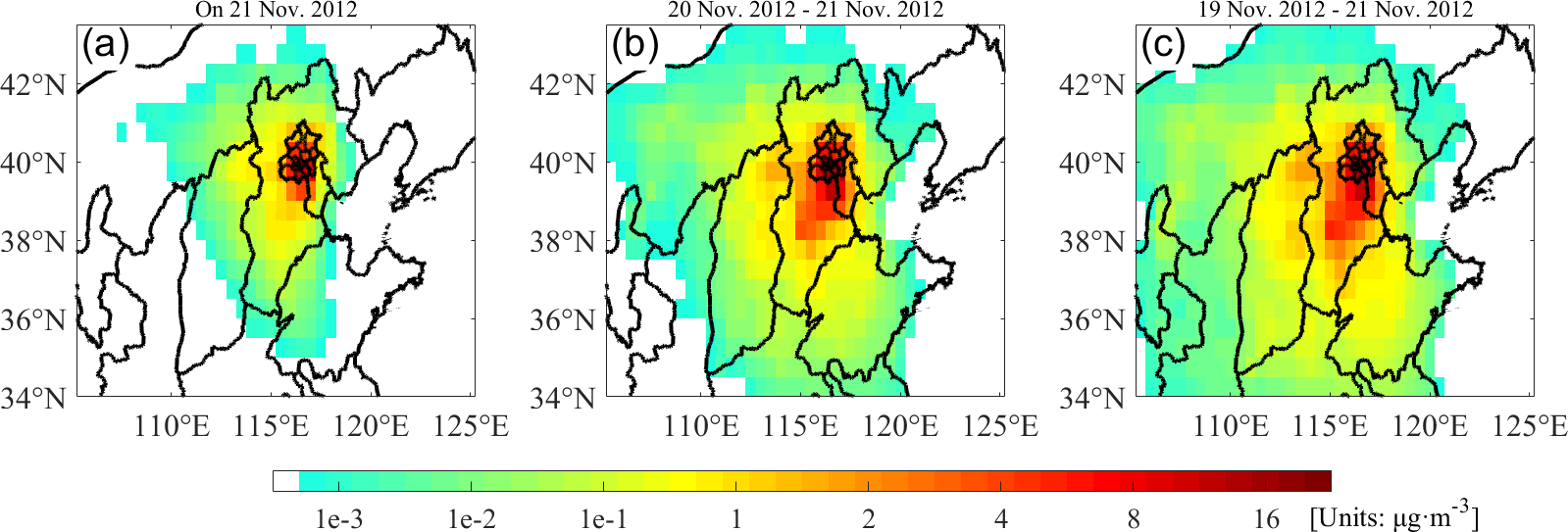
Figure 13The 24 (a), 48 (b), and 72 h (c) integrated sensitivity coefficients of surface PM2.5 concentrations to primary emission sources in Beijing on 21 November 2012.

Figure 14Domain definition of Huabei (HuaB, in red dot-dashed frame), Beijing (BJ, in black solid frame), sensitive Beijing (BJ-sens, red shaded), sensitive Huabei (HuaB-sens, both red and blue shaded), and emission-intensive (Emis-intensive, in pink solid frame) regions.
It is worth noting that, except for the maximal sensitivity coefficients of HB and TJ observed at 16:00 LT on 21 November (7 h ahead of 23:00 LT on 21 November), prior sensitivity coefficient maximal points for the PM2.5 concentration peak observed at 23:00 LT on 21 November appeared at the same time as the maximal points of sensitivity coefficients when the PM2.5 concentration peak observed at 05:00 LT on 21 November was set as the cost function. For example, for both PM2.5 concentration peaks, sensitivity coefficients of TJ emission sources reached a maximal point at 16:00 LT on 20 November, and SX emission source sensitivity coefficients in turn showed two maximal points at 20:00 LT on 20 November and at 20:00 LT on 19 November. The situations at HB and SD are similar: even when maximal points do not appear at the exact same time, high value periods are consistent for the two cost functions. The above phenomenon again revealed that the PM2.5 concentration peak observed at 23:00 LT on 21 November was cumulative on the basis of the PM2.5 concentration peak observed at 05:00 LT on 21 November and that if the PM2.5 concentration peak at 05:00 LT on 21 November can be effectively reduced, the PM2.5 concentration peak at 23:00 LT on 21 November can be reduced accordingly, thus decreasing the overall PM2.5 concentrations on 21 November. These results also reflected the advantage of the adjoint model in detecting spatiotemporal sensitive emission sources in detail.
Figure 12c and d show that along the backward time sequence, the time-integrated sensitivity coefficients of HB continuously rose after the time-integrated sensitivity coefficients of other provinces were prone to remain constant. At around 02:00 to 03:00 LT on 20 November, the time-cumulated emissions influence from HB exceeded that from local BJ emissions for both PM2.5 concentration peaks, thus reflecting that emissions from HB played a leading role in pollutant accumulation for the first BJ PM2.5 concentration peak and that the influence of local emissions was dominant between the two PM2.5 concentration peaks, that is, during the daytime on 21 November.
The hourly sensitivity coefficients in Fig. 12a and b show that the impact of emission sources from Beijing and each surrounding province decreased to negligible values (close to zero) 72 h ahead of the objective time points. Meanwhile, corresponding time-integrated sensitivity coefficients in Fig. 12c and d also stopped increasing 72 h prior to the objective time points. Therefore, by integrating sensitivity coefficients 72 h ahead of the two PM2.5 concentration peaks, we can obtain the overall contributing proportions of emission sources from each province to the BJ PM2.5 concentration peaks (Fig. 12e and f). Among all provinces, HB has the largest impact on the two PM2.5 concentration peaks, and the contribution of HB emissions to the first PM2.5 concentration peak (43.6 %) was greater than to the second PM2.5 concentration peak (41.5 %). For the 05:00 LT PM2.5 concentration peak, the second largest emission source contribution was from Beijing (31.2 %), followed by SX (9.8 %), TJ (9.8 %), and SD (5.7 %); for the 23:00 LT PM2.5 concentration peak, the second largest emission source contribution was from Beijing (35.7 %), followed by SX (8.1 %), SD (8.0 %), and TJ (6.7 %).
From all the above analysis, we can conclude that joint management control of air pollution sources in Hebei province, the city of Tianjin, and Shandong and Shanxi provinces 2 to 3 days ahead of the first PM2.5 concentration peak can effectively reduce PM2.5 concentration accumulation resulting from the transport of pollutants, thus decreasing the BJ PM2.5 concentration peaks.
4.5 Comparisons of the adjoint results with Models-3/CMAQ assessments
Prior research used a back-trajectory model, namely, FLEXPART, to locate sensitive emission regions of Yanqihu, Beijing, on November 2012. The study then used the Models-3/CMAQ modeling system to quantify the effects of emission reduction schemes at different ratios, during different time periods, and over different regions on the reduction of PM2.5 concentrations on 21 November in Beijing (Zhai et al., 2016). On the basis of these results, we set the average PM2.5 concentration over the municipality on 21 November as the cost function and compared the adjoint results with the Models-3/CMAQ assessments. Figure 13 illustrates the time-integrated sensitivity coefficient distributions when the Beijing average PM2.5 concentration on 21 November was set as the cost function. The magnitudes of the sensitivity coefficients reflect the incremental influence of primary emission sources on the objective PM2.5 concentrations. Similar to previous research (Zhai et al., 2016) that advocated the joint management control of emissions with the surrounding provinces 2 to 3 days ahead of the most polluted day, adjoint time-integrated sensitivity was intensified and extended during the 48 to 72 h backward time integration.
To assess the effect of the adjoint sensitive source zone on decreasing PM2.5 concentrations over Beijing and to compare the adjoint results with the Models-3/CMAQ assessments, we looked to the research by Zhai et al. (2016) and selected four emission regions: the overall Huabei region (HuaB), the sensitive Huabei region (HuaB-sens), the overall Beijing municipality (BJ), and the sensitive Beijing region (BJ-sens; Fig. 14). Grid cells with 72 h cumulative sensitivity coefficients larger than 3 µg m−3 were included in the sensitive emission regions (HuaB-sens and BJ-sens), and grid cells with smaller sensitive values are outside the sensitive emission regions. Therefore, sensitive emission regions have relatively larger impact on the PM2.5 peak concentrations than regions outside them. Here the HuaB-sens accounts for 10.2 % of the area of HuaB and the BJ-sens accounts for 60.0 % of the area of BJ, thus making them analogous to the regions defined by Zhai et al. (2016). In the work by Zhai et al. (2016), HuaB-sens accounted for 17.6 % of the area of HuaB and BJ-sens accounted for 54.2 % of the area of BJ. Furthermore, on the basis of the emission magnitudes (Fig. 5), we defined regions with emission intensities larger than 4. g s−1 within HuaB as the “Emis-intensive” regions (Fig. 14). The Emis-intensive region has the same area as that of the HuaB-sens.
Table 3Emission source contribution to the average PM2.5 concentration over Beijing on 21 November.
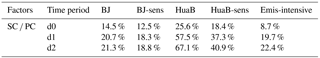
Note that d0 refers to emission contributions from 21 November; d1, 20 to 21 November; d2, 19 to 21 November. SC ∕ PC = time cumulative sensitivity coefficient ∕ peak concentration;
Table 3 lists the ratios of the time cumulative sensitivity coefficients to peak PM2.5 concentrations (SC ∕ PC) from the BJ, BJ-sens, HuaB, HuaB-sens, and Emis-intensive regions at three different time points: d0 (referring to emission contributions from 21 November), d1 (from 20 to 21 November), and d2 (from 19 to 21 November) in advance of the most polluted day. The SC ∕ PC reflects the reduction ratios of peak PM2.5 concentrations due to the absence of emissions from different regions and during different periods, that is, emission source contribution ratios to peak PM2.5 concentrations. From Table 3, we can see that the adjoint model results are highly consistent with the Models-3/CMAQ system results (Zhai et al., 2016). The PM2.5 concentrations on 21 November reflect an accumulated result from emissions released in the 1 or 2 days prior to the most polluted day rather than a simple result of emissions on 21 November. For all the BJ, BJ-sens, HuaB, and HuaB-sens regions, emission contribution ratios grew from d0 to d2, particularly from d0 to d1. The contribution ratios of emissions from BJ (and BJ-sens) and HuaB (and HuaB-sens) increased by 6.2 % (5.8 %) and 31.9 % (18.9 %) from d0 to d1, respectively. Thereafter, the contribution ratios again increased by 0.6 % (0.5 %) and 9.6 % (3.6 %), respectively, for emissions over BJ (or BJ-sens) and HuaB (or HuaB-sens) from d1 to d2. The above phenomenon also indicates that with the accumulation of time-reversed integration from 48 to 72 h prior to 21 November, emission source contributions from HuaB (or HuaB-sens) to peak PM2.5 concentrations increased more obviously, whereas emission source contributions from BJ (or BJ-sens) hardly increased at all. This can be explained by surrounding emissions being continuously transported to Beijing 2 to 3 days ahead of the most polluted day (Zhai et al., 2016).
Table 4Contrast of sensitive (or Emis-intensive) and full region emission source contributions.
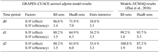
Note that S / F (effect) is the sensitivity coefficient over the sensitive source region / the sensitivity coefficient over the corresponding full source region; contribution efficiency is the sensitivity coefficient / number simulation grid cells in the region; S / F (efficiency) is the contribution efficiency of the sensitive region / the contribution efficiency of the corresponding full source region.
Similar to the work in Models-3/CMAQ assessments, Table 4 shows comparisons of sensitive emission, full emission, and Emis-intensive region source contribution effects and efficiencies to peak PM2.5 concentrations. In Table 4, S / F (effect) in the BJ-sens column refers to the ratios of sensitivity coefficients from BJ-sens to sensitivity coefficients from BJ, and S / F (effect) in the HuaB-sens (or the Emis-intensive) column refers to the ratios of sensitivity coefficients from HuaB-sens (or Emis-intensive) to sensitivity coefficients from HuaB. Correspondingly, S / F (efficiency) refers to the ratios of sensitivity coefficients per unit area from BJ-sens (or from HuaB-sens and Emis-intensive) to sensitivity coefficients per unit area from BJ (or from HuaB). Therefore, S / F (effect) and S / F (efficiency) reflect emission source reduction effects and reduction efficiency from critical (or emission-intensive) regions. The implication of d0, d1, and d2 results in Table 4 are the same as they are in Table 3. As shown in Table 4, the contribution efficiencies (contribution ratios per unit area) of emissions from the HuaB-sens and BJ-sens regions are significantly higher than those from the corresponding entire HuaB and BJ regions, respectively. Although BJ-sens covers only 60 % of the area of the entire BJ, its contribution to the peak PM2.5 concentrations is 86.6–88.2 % of that of the entire BJ. Its source contribution efficiency is 1.4 to 1.5 times that of BJ. Similarly, HuaB-sens covers only 10.2 % of the area of the entire HuaB, but its contribution to the peak PM2.5 concentrations is 61.0–71.9 % of that of the entire HuaB, and its source contribution efficiency is 6.0 to 7.0 times that of the entire HuaB (Table 4). Finally, emissions from HuaB-sens contribute much more than emissions only from BJ-sens, which supports joint management control. Analogously, in the Models-3/CMAQ assessments, BJ-sens (or HuaB-sens) covers 54.2 % (or 17.6 %) of the area of BJ (or HuaB), its emission reduction effect is 99.2–100 % (or 87.2–93.7 %) of that of the entire BJ (or HuaB), and its source contribution efficiency is 1.8 to 1.9 times (or 5.0 to 5.3 times) that of BJ (or HuaB).
We then compared emission source contribution ratios, effects, and efficiencies from the HuaB-sens and the Emis-intensive regions. As shown in Tables 3 and 4, although the Emis-intensive region has the same area as HuaB-sens, its SC ∕ PC, S / F (effect), and S / F (efficiency) values are all much smaller. The source contribution ratios to PM2.5 concentrations on 21 November (SC ∕ PC) from the Emis-intensive regions are 9.7, 17.6, and 18.5 % smaller, respectively, than those from HuaB-sens (Table 3), and the source contribution effect from the Emis-intensive regions (S / F (effect)) are 37.9, 30.7, and 27.6 % smaller, respectively, than the S / F (effect) of HuaB-sens, thus indicating that controlling air pollution sources from adjoint critical emission regions has better effects and higher efficiency than controlling emission sources from emission-intensive regions.
The computational loads of the adjoint simulation were much smaller than the comparable assessments made with the Models-3/CMAQ modeling (Zhai et al., 2016). For the adjoint simulation, one forward integration (for model state variables saving) and one backward adjoint integration can enable the determination of the influence of emissions from any source region during any time period to PM2.5 concentration peaks. For the Models-3/CMAQ assessments, to compare the effects of emission reductions over two different time periods at two different ratios and from four different regions, 12 sensitivity tests with a control simulation are required. Although the deficiency of the adjoint analysis in this study is that we did not include PM2.5 concentration precursor emission impacts, we find through comparison that the two modeling approaches are highly comparable in their assessments of atmospheric pollution control for critical emission regions. Overall, the adjoint sensitivities of peak PM2.5 concentrations to primary PM2.5 emissions using the GRAPES–CUACE aerosol adjoint model can provide a valuable reference for evaluating emission impacts on pollutant concentrations and air quality control.
In this research, the GRAPES–CUACE aerosol adjoint model was applied to detect the pivotal emission sources of a November 2012 haze episode over Beijing, and the hourly peak PM2.5 concentrations at 05:00 and 23:00 LT on 21 November 2012 were set as the cost functions. The peak PM2.5 concentration contributions from local Beijing emissions and neighboring provinces were well compared. The adjoint model results corresponded well with the real weather analysis for this period and correctly described the spatial distribution of the most influential emission sources over time for both PM2.5 concentration peaks. The 05:00 LT PM2.5 concentration peak was mainly influenced by local Beijing emissions and the emissions from Hebei, Tianjin, and Shanxi because of the transmission of pollutants 2 to 3 days ahead of the peak time. The 23:00 LT PM2.5 concentration peak was more sensitive to local Beijing emissions, and the regions to the south of Beijing in Hebei province, because of the accumulation from the first PM2.5 concentration peak, local particle hygroscopic growth, and pollutants trapped against of the Taihang Mountains on 21 November. The upstream Hebei province has the largest impact on both PM2.5 concentration peaks, and the contribution of Hebei emissions to the first PM2.5 concentration peak (43.6 %) was greater than that to the second PM2.5 concentration peak (41.5 %). In Beijing, PM2.5 concentration peaks responded to local emissions in 1 to 2 h, whereas surrounding emissions took 7 to 12 h to influence Beijing's air quality. The relationship between PM2.5 and their primary emission sources is complicated by different weather conditions. Aerosol impacts on meteorological fields could be significant, which might further affect the aerosol pollution condition in the lower troposphere. Also, aerosol–cloud interactions might modify temperature and moisture profiles and precipitation (Wang et al., 2011), leading to potential feedback on the atmospheric chemistry. Moreover, climate change also has potential impacts on the pollution conditions in China (Wu et al., 2016). Further studies are required to investigate the relationship of adjoint sensitivities' representation of emission source contribution under different weather conditions.
We compared the adjoint results with Models-3/CMAQ assessments and found that the adjoint model results can provide evidence for all the conclusions supported by the Models-3/CMAQ assessments (Zhai et al., 2016). We then defined the Emis-intensive region as an emission-intensive region within the Huabei region that has the same area as that of sensitive Huabei region (HuaB-sens) and compared its emission source contributions with those of HuaB-sens and HuaB. Overall, we concluded that narrowing the emission sources reduction scope to target critical source zones (zones detected by an adjoint model or a FLEXPART model), rather than emission-intensive regions, 2 to 3 days prior to unfavorable meteorological conditions can effectively decrease PM2.5 concentrations and improve the efficiency of PM2.5 reduction measures. Meanwhile, the adjoint simulation is far more computationally efficient than the assessments with Models-3/CMAQ modeling. The adjoint method is a powerful tool for simulating the relationship between emissions and concentrations, and it can be utilized to help improve flexible air quality control schemes. As we are now coupling the CB-IV mechanism in the GRAPES–CUACE forward model and embedding the CB-IV adjoint into the adjoint of GRAPES–CUACE, we will estimate sensitivities to both primary and precursor gaseous emission sources after this development.
Data are available from Shixian Zhai (zhaisx0605@163.com), Xingqin An (anxq@camscma.cn) or Tianliang Zhao (tlzhao@nuist.edu.cn) upon request.
The supplement related to this article is available online at: https://doi.org/10.5194/acp-18-6241-2018-supplement.
The authors declare that they have no conflict of interest.
This work was supported by the National Nature Science Foundation of China
(grant nos. 41575151 and 91644223), the National Key R&D Program Pilot
Projects of China (grant no. 2016YFC0203304), the China Scholarship Council and the Program for Postgraduate Research Innovation of Jiangsu
Higher Education Institutions (grant no.
KYZZ16_0346).
Edited by: Renyi Zhang
Reviewed by: four anonymous referees
An, X., Zhu, T., Wang, Z., Li, C., and Wang, Y.: A modeling analysis of a heavy air pollution episode occurred in Beijing, Atmos. Chem. Phys., 7, 3103–3114, https://doi.org/10.5194/acp-7-3103-2007, 2007.
An, X. Q., Sun, Z. B., Lin, W. L., Jin, M., and Li, N.: Emission inventory evaluation using observations of regional atmospheric background stations of China, J. Environ. Sci., 25, 537–546, 2013.
An, X. Q., Zhai, S. X., Jin, M., Gong, S., and Wang, Y.: Development of an adjoint model of GRAPES–CUACE and its application in tracking influential haze source areas in north China, Geosci. Model Dev., 9, 2153–2165, https://doi.org/10.5194/gmd-9-2153-2016, 2016.
Boylan, J. W. and Russell, A. G.: PM and light extinction model performance metrics, goals, and criteria for three-dimensional air quality models. Atmos. Environ., 40, 4946–4959, 2006.
Cao, G. L., Zhang, X. Y., Gong, S. L., An, X. Q., and Wang, Y. Q.: Emission inventories of primary particles and pollutant gases for China, Chinese Sci. Bull., 56, 781–788, https://doi.org/10.1007/s11434-011-4373-7, 2011.
Carmichael, G. R., Sandu, A., Chai, T. F., Daescu, N. D., Constantinescu, E. M., and Tang Y. H.: Predicting air quality: Improvements through advanced methods to integrate models and measurements, J. Comput. Phys., 227, 3540–3571, 2008.
Constantin, B. V. and Barrett, S. R.: Application of the complex step method to chemistry-transport modeling, Atmos. Environ., 99, 457–465, 2014.
Chen, Z. Y., Xu, B., Cai, J., and Gao, B. B.: Understanding temporal patterns and characteristics of air quality in Beijing: A local and regional perspective, Atmos. Environ., 127, 303–315, 2016.
Cheng, Y., Zheng, G., Wei, C., Mu, Q, Zheng, B., Wang, Z., Gao, M., Zhang, Q., He, K., Carmichael, G., Pöschl, U., and Su, H.: Reactive nitrogen chemistry in aerosol water as a source of sulfate during haze events in China, Science Advances, 2, e1601530, https://doi.org/10.1126/sciadv.1601530, 2016.
Errico, R. M.: What is an adjoint model?, B. Am. Meteorol. Soc., 78, 2577–2591, 1997.
Gao, M., Carmichael, G. R., Wang, Y., Saide, P. E., Yu, M., Xin, J., Liu, Z., and Wang, Z.: Modeling study of the 2010 regional haze event in the North China Plain, Atmos. Chem. Phys., 16, 1673–1691, https://doi.org/10.5194/acp-16-1673-2016, 2016.
Gong, S. L., Barrie, L. A., Blanchet, J.-P., Salzen, K. v., Lohmann,U., Lesins, G., Spacek, L., Zhang, L. M., Girard, E., and Lin, H.: Canadian Aerosol Module: A size-segregated simulation of atmospheric aerosol processes for climate and air quality models, 1, Module development, J. Geophys. Res., 108, 4007, https://doi.org/10.1029/2001JD002002, 2003.
Guo, S., Hu, M., Zamora M. L., Peng, J. F., Shang, D. J., Zheng, J., Du, Z. F., Wu, Z. J., Shao, M., Zeng, L. M., Molina, M. J., and Zhang, R. Y.: Elucidating severe urban haze formation in China, P. Natl. Acad. Sci. USA, 111, 17373–17378, 2014.
Guo, Y. M., Tong, S. L., Li, S. S., Barnett, A. G., Yu, W. W., Zhang, Y. S., and Pan, X. C.: Gaseous air pollution and emergency hospital visits for hypertension in Beijing, China: a time-stratified case-crossover study, Environ. Health-Glob., 9, 57, https://doi.org/10.1186/1476-069X-9-57, 2010.
Hakami, A., Henze, D. K., Seinfeld, J. H., Singh, K., Sandu, A., Kim, S., Byun, D., and Li, Q.: The adjoint of CMAQ, Environ. Sci. Technol., 41, 7807–7817, 2007.
Henze, D. K., Hakami, A., and Seinfeld, J. H.: Development of the adjoint of GEOS-Chem, Atmos. Chem. Phys., 7, 2413–2433, https://doi.org/10.5194/acp-7-2413-2007, 2007.
Henze, D. K., Seinfeld, J. H., and Shindell, D. T.: Inverse modeling and mapping US air quality influences of inorganic PM2.5 precursor emissions using the adjoint of GEOS-Chem, Atmos. Chem. Phys., 9, 5877–5903, https://doi.org/10.5194/acp-9-5877-2009, 2009.
Jiang, C., Wang, H., Zhao, T., Li, T., and Che, H.: Modeling study of PM2.5 pollutant transport across cities in China's Jing-Jin-Ji region during a severe haze episode in December 2013, Atmos. Chem. Phys., 15, 5803–5814, https://doi.org/10.5194/acp-15-5803-2015, 2015.
Li, L. J., Wang, Z. S., Zhang, D. W., Chen, T., Jiang, L., and Li, Y. T.: Analysis of heavy air pollution episodes in Beijing during 2013–2014, China Environmental Science, 36, 27–35, 2016 (in Chinese).
Liu, Z., Hu, B., Wang, L., Wu, F., Gao, W., and Wang, Y.: Seasonal and diurnal variation in particulate matter (PM10 and PM2.5) at an urban site of Beijing: analyses from a 9-year study, Environ. Sci. Pollut. R., 22, 627–642, 2015.
Marchuk, G. I.: Numerical Solution of the Problems of the Dynamics of the Atmosphere and Ocean, J. Baltimore College of Dental Surgery, 22, 28–55, 1974.
Marchuk, G.: Mathematical Models in Environmental Problems, Elsevier Science Publishers, New York, 1986.
Sandu, A., Daescu, D. N., Carmichael, G. R., and Chai, T.: Adjoint sensitivity analysis of regional air quality models, J. Comput. Phys., 204, 222–252, 2005.
Sun, Y. L., Jiang, Q., Wang, Z., Fu, P. Q., Li, J., Yang T., and Yin, Y.: Investigation of the sources and evolution processes of severe haze pollution in Beijing in January 2013, J. Geophys. Res.-Atmos., 119, 4380–4398, 2014.
Stockwell, W. R., Middleton, P., Change, J. S., and Tang, X.: The second generation regional acid deposition model chemical mechanism for regional air quality modeling. J. Geophys. Res. 95, 16343–16376, 1990.
Tang, G., Zhang, J., Zhu, X., Song, T., Münkel, C., Hu, B., Schäfer, K., Liu, Z., Zhang, J., Wang, L., Xin, J., Suppan, P., and Wang, Y.: Mixing layer height and its implications for air pollution over Beijing, China, Atmos. Chem. Phys., 16, 2459–2475, https://doi.org/10.5194/acp-16-2459-2016, 2016.
Wang, G., Zhang, R., Gomez, M. E., et al.: Persistent sulfate formation from London Fog to Chinese haze, P. Natl. Acad. Sci. USA, 113, 13630–13635, 2016.
Wang, H., Gong, S. L., Zhang, H. L., Chen, Y., Shen, X. S., Chen, D. H., Xue, J. S., Shen, Y. F., Wu, X. J. and Jin, Z. Y.: A new-generation sand and dust storm forecasting system GRAPES_CUACE/Dust: Model development, verification and numerical simulation, Chinese Sci. Bull., https://doi.org/10.1007/s11434-009-0481-z, 2009.
Wang, H., Shi, G. Y., Zhang, X. Y., Gong, S. L., Tan, S. C., Chen, B., Che, H. Z., and Li, T.: Mesoscale modelling study of the interactions between aerosols and PBL meteorology during a haze episode in China Jing–Jin–Ji and its near surrounding region – Part 2: Aerosols' radiative feedback effects, Atmos. Chem. Phys., 15, 3277–3287, https://doi.org/10.5194/acp-15-3277-2015, 2015a.
Wang, H., Shi, G. Y., Zhang, X. Y., Gong, S. L., Tan, S. C., Chen, B., Che, H. Z., and Li, T.: Mesoscale modelling study of the interactions between aerosols and PBL meteorology during a haze episode in China Jing-Jin-Ji and its near surrounding region – Part 2: Aerosols' radiative feedback effects, Atmos. Chem. Phys., 15, 3277–3287, https://doi.org/10.5194/acp-15-3277-2015, 2015b.
Wang, L. T., Wei, Z., Wei, W., Fu, J. S., Meng, C. C., and Ma, S.: Source apportionment of PM2.5 in top polluted cities in Hebei, China using the CMAQ model, Atmos. Environ., 122, 723–736, 2015.
Wang, Y., Wan, Q., Meng, W., Liao, F., Tan, H., and Zhang, R.: Long-term impacts of aerosols on precipitation and lightning over the Pearl River Delta megacity area in China, Atmos. Chem. Phys., 11, 12421–12436, https://doi.org/10.5194/acp-11-12421-2011, 2011.
Wu, D., Xu, Y., and Zhang S. Q.: Will joint regional air pollution control be more cost-effective? An empirical study of China's Beijing–Tianjin–Hebei region, J. Environ. Manage., 149, 27–36, 2015.
Wu, G. X., Li, Z. Q., Fu, C. B., Zhang, X. Y., Zhang, R. Y., Zhang, R. H., Zhou, T. J., Li, J. P., Li, J. D., Zhou, D. G., Wu, L., Zhou, L. T., He, B., and Huang, R. H.: Advances in studying interactions between aerosols and monsoon in China, Science China Earth Sciences, 59, 1–16, 2016.
Xue, J. and Chen, D.: Scientific Design and Application of Numerical Predicting System GRAPES, Science Press, Beijing, 2008.
Zhai, S. X.: Development of the Adjoint of GRAPES-CUACE Aerosol Module and Model Application to Air Pollution Optimal Control Problems, Master dissertation, Chinese Academy of Meteorological Sciences, Beijing, 2015 (in Chinese).
Zhai, S. X., An, X. Q., Liu, Z., Sun, Z. B., and Hou, Q.: Model assessment of atmospheric pollution control schemes for critical emission regions, Atmos. Environ., 124, 367–377, 2016.
Zhang, H. F., Wang, S. X., Hao, J. M., Wang, X. M., Wang, S. L., Chai, F. H., and Li, M.: Air pollution and control action in Beijing, J. Clean. Prod., 112, 1519–1527, 2016.
Zhang, L., Liu, L. C., Zhao, Y. H., Gong, S. L., Zhang, X. Y., Henze, D. K., Capps, S. L., Fu, T. M., Zhang, Q., and Wang, Y. X.: Source attribution of particulate matter pollution over North China with the adjoint method, Environ. Res. Lett., 10, 084011, https://doi.org/10.1088/1748-9326/10/8/084011, 2015.
Zhang, R. Y., Wang, G. H., Guo, S., Zamora, M. L., Ying, Q., Lin, Y., Wang, W. G., Hu, M., and Wang, Y.: Formation of Urban Fine Particulate Matter, Chem. Rev., 115, 3803–3855, 2015.
Zhou, C. H., Gong, S. L., Zhang, X. Y., Liu, H. L., Xue, M., Cao, G. L., An, X. Q., Che, H. Z., Zhang, Y. M., and Niu, T.: Towards the improvements of simulating the chemical and optical properties of Chinese aerosols using an online coupled model – CUACE/Aero, Tellus B, 64, 18965, https://doi.org/10.3402/tellusb.v64i0.18965, 2012.