Nonlinear response of tropical lower-stratospheric temperature and water vapor to ENSO

A series of simulations using the NASA Goddard Earth Observing System Chemistry–Climate Model are analyzed in order to aid in the interpretation of observed interannual and sub-decadal variability in the tropical lower stratosphere over the past 35 years. The impact of El Niño–Southern Oscillation on temperature and water vapor in this region is nonlinear in boreal spring. While moderate El Niño events lead to cooling in this region, strong El Niño events lead to warming, even as the response of the large-scale Brewer–Dobson circulation appears to scale nearly linearly with El Niño. This nonlinearity is shown to arise from the response in the Indo-West Pacific to El Niño: strong El Niño events lead to tropospheric warming extending into the tropical tropopause layer and up to the cold point in this region, where it allows for more water vapor to enter the stratosphere. The net effect is that both strong La Niña and strong El Niño events lead to enhanced entry water vapor and stratospheric moistening in boreal spring and early summer. These results lead to the following interpretation of the contribution of sea surface temperatures to the decline in water vapor in the early 2000s: the very strong El Niño event in 1997/1998, followed by more than 2 consecutive years of La Niña, led to enhanced lower-stratospheric water vapor. As this period ended in early 2001, entry water vapor concentrations declined. This effect accounts for approximately one-quarter of the observed drop.

1 Introduction

The El Niño–Southern Oscillation (ENSO) is the largest source of interannual variability in the tropics and manifests as anomalous sea surface temperatures (SSTs) in the eastern and central Pacific Ocean. El Niño (EN), the phase with anomalously warm SSTs in this region, has been shown to impact stratospheric temperatures in both the polar region and in the tropics (Calvo Fernández et al., 2004; Sassi et al., 2004; Manzini et al., 2006; Garcia-Herrera et al., 2006; Taguchi and Hartmann, 2006; Garfinkel and Hartmann, 2007; Marsh and Garcia, 2007; Free and Seidel, 2009; Calvo et al., 2010). The temperature response in these two regions is linked, as ENSO is able to modify the stratospheric mean meridional circulation, also known as the Brewer–Dobson circulation (BDC). During most EN events, anomalous upward propagation and dissipation of planetary waves at middle and high latitudes, and gravity waves and transient synoptic waves in the subtropics (Garfinkel and Hartmann, 2008; Calvo et al., 2010; Simpson et al., 2011), lead to the acceleration of the BD circulation, resulting in a cooler tropical lower stratosphere and warmer polar stratosphere.

In addition to impacting zonal mean tropical lower-stratospheric temperatures, ENSO also impacts the zonal distribution of temperature anomalies. EN leads to a Rossby wave response whereby anomalously warm temperatures are present over the Indo-Pacific warm pool near the tropopause, with colder temperatures further east over the central Pacific (Yulaeva and Wallace, 1994; Randel et al., 2000; Zhou et al., 2001; Scherllin-Pirscher et al., 2012). In the tropical tropopause layer water vapor increases in the region with warm anomalies and decreases in the region with cold anomalies, and these local changes in tropical water vapor can exceed 25 % below the cold point (Gettelman et al., 2001; Hatsushika and Yamazaki, 2003; Konopka et al., 2016).

The net effect of these temperature anomalies on water vapor above the tropical cold point is complex, as these zonally asymmetric changes are superposed on the larger-scale warming or cooling associated with changes of the BDC. The two largest EN events in the satellite era (in 1997/1998 and in 2015/2016) clearly preceded moistening of the tropical lower stratosphere (Fueglistaler and Haynes, 2005; Avery et al., 2017), though the impact of more moderate events is less clear. The net effect of EN on water vapor at the cold point is the residual of the large temperature anomalies in the western Pacific and central Pacific (Gettelman et al., 2001; Davis et al., 2013; Konopka et al., 2016), and zonally averaged changes in entry water vapor for the ENSO events considered by Gettelman et al. (2001) is 0.1 ppmv. In addition, Calvo et al. (2010), Garfinkel et al. (2013a), and Konopka et al. (2016) note the strong seasonal dependence of the effect of EN on stratospheric water vapor: only in boreal spring does EN lead to enhanced water vapor and La Niña (LN) to dehydration, and Garfinkel et al. (2013a) relate this to seasonality in the collocation of the warm anomalies forced by EN with the coldest region near the cold point tropopause.

An additional complexity is the relationship between oceanic temperatures in the Pacific and Indian oceans during ENSO events. EN leads to warming in the Indian Ocean in the boreal spring following the peak SST anomalies in the Pacific Ocean (Webster et al., 1999; Murtugudde et al., 2000; Su et al., 2001; Schott et al., 2009). However, this relationship between Indian Ocean and Pacific Ocean SSTs is not universal: while the 1997/1998 event was followed by unusually warm Indian Ocean SSTs (Webster et al., 1999; Yu and Rienecker, 2000; Murtugudde et al., 2000), the 1982/1983 event was followed by moderate warming despite comparable anomalies in the Niño-3.4 region of the Pacific Ocean. Teleconnections of EN in boreal spring and summer can be driven both by the Indian Ocean warming and by any lingering SST anomalies in the Pacific. For example, previous work has shown that impacts of EN in parts of East Asia are dominated by the Indian Ocean warming (Xie et al., 2009), while the Arctic stratospheric response to EN is damped by the Indian Ocean warming (Fletcher and Kushner, 2011). It is not clear to what extent the tropical stratospheric response to ENSO, particularly in boreal spring, is governed by these Indian Ocean anomalies and not by any lingering anomalies in the Pacific.

A clearer understanding of the role of ENSO for entry water vapor may be important for understanding the drop in water vapor in the early 2000s (Randel et al., 2004, 2006): Brinkop et al. (2016) argue that the evolution of ENSO from 1997 through 2000 was crucial for this event. As the amount of water vapor that enters the stratosphere is important for stratospheric chemistry (Solomon et al., 1986) and radiative balance (Forster and Shine, 1999; Solomon et al., 2010), it is important to understand the factors that control its entry into the stratosphere on all timescales.

This paper is motivated by four specific issues related to the lower-stratospheric response to ENSO: first, a commonly used method to ascribe stratospheric variability to forcings such as ENSO, the quasibiennial oscillation (QBO), solar variability, and volcanoes is to use multiple linear regression (e.g., Crooks and Gray, 2005; Marsh and Garcia, 2007; Mitchell et al., 2015). An assumption underlying this method is that the response to these forcings is linear, i.e., that the response to a given magnitude EN is equal and opposite to that of a LN event of equal magnitude. Is this assumption really true? Second, Garfinkel et al. (2013a) found that EN events whose SST anomalies peak in the central Pacific (i.e., CP events) lead to dehydration regardless of season while events peaking in the eastern Pacific (i.e., EP events) lead to boreal spring moistening. However, EP events tend to be stronger than CP events, and it is not clear to what extent the difference found by Garfinkel et al. (2013a) reflects the intensity of the EN event or the flavor of the event. Third, to what extent is the tropical stratospheric response to ENSO governed by SST anomalies in the Indian Ocean sector that typically follow (though with diversity in their amplitude) ENSO? Finally, it has been suggested that SST variability in the Pacific Ocean contributed to the drop in water vapor in the early 2000s (Rosenlof and Reid, 2008; Garfinkel et al., 2013b) possibly via ENSO (Brinkop et al., 2016), but this contribution has not yet been quantified except by one very recent study (Ding and Fu, 2017).

This paper will demonstrate that there are nonlinearities in the lower-stratospheric temperature and water vapor response to ENSO. While typical EN events lead to tropical lower-stratospheric cooling and dehydration in boreal winter, the spring response is nonlinear: strong EN events and LN lead to moistening while weak or moderate EN events lead to dehydration. We clarify that discriminating between CP and EP events may not be crucial, and rather one should discriminate between very strong EN events and moderate EN events. As CP events tend to be weaker than EP events (Johnson, 2013), it is easy to confuse a composite of CP EN events with a composite of moderate EN regardless of type. This nonlinearity apparently originates in the Indo-West Pacific response to EN, as warming in this region leads to moistening of the stratosphere in spring. Finally, by comparing changes in water vapor concentrations between the early 2000s and late 1990s in a large ensemble of model simulations forced with observed SSTs, we suggest that the deterministic component of the water vapor drop in the early 2000s was 0.14 ppmv, approximately one-quarter of the observed drop.

A complete explanation of interannual variability in stratospheric water vapor, particularly that associated with EN, requires consideration of changes in both temperature and air-parcel trajectories near the tropopause (Bonazzola and Haynes, 2004; Hasebe and Noguchi, 2016; Konopka et al., 2016), and might also be influenced by changes in cloud ice (Avery et al., 2017). We cannot distinguish among these various effects in our simulations since the model output necessary to run a Lagrangian trajectory model was not archived. Nonetheless all of these effects operate in the simulations, and the simulated interannual variability in water vapor will arise from some combination of these effects.

More generally, the objective behind studying historical changes in water vapor and temperature in free running climate simulations is not to form a best estimate of the actual interannual variability; for that purpose, nudged experiments and/or Lagrangian trajectory modeling are far better. Rather, the motivation is threefold: one, assuming the model is capable of capturing interannual variability, the causes of trends or discontinuities (such as the drop in the early 2000s) can be better understood in a framework in which there is no possibility that changes in the observing or modeling system could have led to these trends or discontinuities; two, large ensembles of a free running model can be produced in order to better isolate the forced response from a single EN event from unrelated internal atmospheric variability not forced by anomalies at the ocean surface; three, and relatedly, the observational record is not long enough in order to confidently conclude whether the response to ENSO is nonlinear or to confidently separate the impacts of Indian Ocean SSTs from Pacific SSTs due to their strong co-variability, and thus only by considering large model ensembles can these effects be confidently identified.

The data and methods are introduced in Sects. 2 and 3. Section 4 demonstrates the nonlinearity of ENSO's effect on tropical lower-stratospheric temperature and water vapor. In order to better understand the nonlinearity evident in Sect. 4, Sect. 5 more closely considers the strongest EN event covered by our model experiments – the event in 1997/1998 – and highlights the importance of the Indian Ocean. Section 6 considers implications for the drop in the early 2000s and for the EN event in 2015/2016. The Supplement discusses the linearity of the influence of ENSO on the BDC.

2 Data

We analyze the MERRA (Modern-Era Retrospective Analysis for Research and Applications;  Rienecker et al., 2011) reanalysis, the merged water vapor product from SWOOSH v2.5 (Davis et al., 2016), and output from atmospheric chemistry–climate general circulation models (GCMs) and coupled ocean–atmosphere GCMs on various timescales. The Goddard Earth Observing System Chemistry–Climate Model, version 2 (GEOSCCM, Rienecker et al., 2008) couples the GEOS-5 (Rienecker et al., 2008; Molod et al., 2012) atmospheric general circulation model to the comprehensive stratospheric chemistry module StratChem (Pawson et al., 2008; Oman and Douglass, 2014). The model has 72 vertical layers, with a model top at 0.01 hPa, and all simulations discussed here were performed at 2^∘ latitude × 2.5^∘ longitude horizontal resolution. The model spontaneously generates a QBO (Molod et al., 2012). The model vertical levels between 140 and 50 hPa are located at 139.1, 118.3, 100.5, 85.4, 72.6, 61.5, and 52.0 hPa; output is plotted at standard pressure levels.

The convection scheme used in GEOSCCM is based on relaxed Arakawa–Schubert (Moorthi and Suarez, 1992; Rienecker et al., 2008), and the cloud ice parameterization is described in Molod et al. (2012). Note that there is cloud ice in the version of the model under consideration here up to 85 hPa (as is shown below). To the extent that entry water vapor is controlled by large-scale temperature patterns and the relatively crude ice parameterization in the current generation of the model, we expect that our model captures the response of water vapor to ENSO. That being said, more advanced treatments of ice clouds are currently under development, and hence similar studies must be performed as models improve.

Li et al. (2016)Garfinkel et al. (2015)Aquila et al. (2016)Aquila et al. (2016)Aquila et al. (2016)Garfinkel et al. (2015)Aquila et al. (2016)Aquila et al. (2016)

Table 1 GEOSCCM model experiments.

A series of integrations were performed with the GEOSCCM, and they are listed in Table 1 and described below. They fall into two classes: coupled ocean–atmosphere simulations, and historical SST simulations with an atmospheric chemistry–climate general circulation model (AGCM). Both modeling frameworks have their advantages: coupled ocean–atmosphere simulations allow the model to self-consistently develop SST anomalies and teleconnections without violating energetic constraints and also allow us to examine the stratospheric response to a wider range of ENSO events than have occurred in the historical record. Conversely, simulations forced with observed SSTs can be more easily compared to the observed response to ENSO.

The model configuration for the coupled ocean–atmosphere simulation is described in Li et al. (2016). The ocean model is the Modular Ocean Model version 5 (Griffies et al., 2015) with 50 vertical layers, and the ocean horizontal resolution is about 1^∘ latitude by 1^∘ longitude. We consider the last 240 years of a 340-year simulation in which greenhouse gas (GHG) and ozone-depleting substance (ODS) forcings are fixed at 1950 levels. Figure 1 compares the 2 m temperatures over the Niño-3.4 region to those over the (top) Indian Ocean and (bottom) Indo-Pacific warm pool region in the coupled model and in MERRA reanalysis data. The model simulates stronger ENSO events than have occurred, similar to the bias in a previous version of this ocean model (Dunne et al., 2012; Capotondi et al., 2015). Biases in climatological zonal wind stress and SSTs in the Pacific are shown in Figs. 3 and 4 of Li et al. (2016); briefly, SSTs in the tropical west and central Pacific are too warm, consistent with zonal wind stresses that are not sufficiently easterly. Regardless of these biases, the tendency of EN events to lead to a warmer Indian Ocean is well captured by the model (Fig. 1ab). The connection between ENSO and the Indo-Pacific warm pool region is similar in both the ERSSTv5 dataset (Huang et al., 2017) that is used in Fig. 1 and in the Met Office Hadley center observational database (Rayner et al., 2006) (not shown).

Figure 1 Relationship between near surface temperatures over the Niño-3.4 region and over the Indian Ocean and western Pacific basins from 5^∘ S to 5^∘ N in (blue) the GEOSCCM coupled ocean–atmosphere integration and in (red) MERRA reanalysis data. The EN event 1982/1983 is indicated with a large red diamond, and the EN event in 1997/1998 is indicated with a large x. (a, c) January through April; (b, d) annual average. (a, b) Indian Ocean from 50 to 100^∘ E; (c, d) Indo-West Pacific from 50 to 150^∘ E.

The foundation of the AGCM ensemble is the simulations discussed by Garfinkel et al. (2015) and Aquila et al. (2016), though several recent integrations have been added, as summarized in Table 1. The simulations form a 42-member ensemble of the period from January 1980 to December 2009, though five integrations have been extended to the near-present to cover the strong EN event in 2015/2016 and one integration ends in December 2008. Such an ensemble is valuable as it frames the forced response to EN common to all integrations within the context of stochastic unforced variability unique to each integration. For 13 integrations, the only time-varying forcings are changing SSTs and sea ice; SSTs and sea ice up to November 2006 are taken from the Met Office Hadley center observational database (Rayner et al., 2006) and from the National Climatic Data Center (Reynolds et al., 2002) since then. For three additional integrations, GHG concentrations are from observations up to 2005 and from the Representative Concentrations Pathway 4.5 after 2005 (Meinshausen et al., 2011) in addition to time-varying SSTs and sea ice. For 19 additional integrations ODSs also vary as observed. For seven additional integrations these forcings plus volcanic eruptions are included (Aquila et al., 2016); for these seven integrations we discard the seasons 1991/1992 and 1992/1993 and the years 1991, 1992, and 1993 from consideration, as the eruption of Mt. Pinatubo had a large impact on the BDC and tropical temperatures in our simulations (Aquila et al., 2016; Garfinkel et al., 2017) and appears to have led to moistening in observational data as well (Fueglistaler, 2012; Dessler et al., 2014). In 1994 the difference in entry water vapor between these seven integrations and the other integrations is less than 0.05 ppmv (not shown). Four of these seven integrations also include time-varying solar forcing. All simulations considered are summarized in Table 1. These simulations have been performed for various purposes and differ in the forcings included and in the physical parameterizations, but they all include changing SSTs and sea ice.

GEOSCCM model output is compared to temperatures from MERRA and water vapor from SWOOSH v2.5. Temperatures from MERRA are interpolated to the same 2^∘ latitude × 2.5^∘ longitude grid used for the GEOSCCM simulations. In order to isolate the interannual variability, we detrend time series for the AGCM simulations and for reanalysis and observations.

Anomalies are computed as follows. A monthly climatology over the full duration of each model experiment, reanalysis product, and observational dataset is computed and is then subtracted from the raw fields to generate monthly anomalies. The model climatology is computed separately for each model simulation due to differences in the forcing agents and model components used.

3 Methods

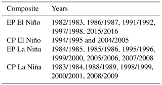
ENSO events are identified based on November through February seasonal mean SST anomalies in the ERSSTv5 dataset (Huang et al., 2017) with a 1981–2010 base period. LN events are identified when SST anomalies in the Niño-3.4 region (5^∘ S–5^∘ N, 170–120^∘ W) are more negative than −0.5 K, while EN events are identified when SST anomalies in this region are larger than 0.5 K. LN and EN events are further categorized into four groups similar to Hurwitz et al. (2014): CP EN, characterized by positive SST anomalies in the Niño-4 region (5^∘ S–5^∘ N, 160–210^∘ E), and EP EN, characterized by positive SST anomalies in the Niño-3 region (5^∘ S–5^∘ N, 210–270^∘ E), as well as CP and EP LN events, characterized by negative SST anomalies in the same two regions. EP LN events are identified when the Niño-3 anomaly is 0.1 K less than the Niño-4 anomaly. Similarly, EP EN events are identified when the Niño-3 anomaly is 0.1 K larger than the corresponding Niño-4 anomaly. CP EN and CP LN events are identified analogously. All remaining years, either because they are neutral ENSO or because the Niño-3 and Niño-4 anomalies are within 0.1 K, are categorized as “other events”. The years included in each composite are listed in Table 2.

Table 2 Events composited for AGCM and observations.

Most ENSO events peak around December and decay through the following spring. Hence, we focus on the response of the lower stratosphere during the period from November through June.

As discussed in the introduction it is well known that EN forces an intensified BDC, and associated with an accelerated BDC are colder tropical lower-stratospheric temperatures and less water vapor. Here we consider the response to ENSO without regressing out the influence of the BDC on water vapor except where indicated, as regressing out the BDC misrepresents the net impact of ENSO on the lower stratosphere. We consider two alternate diagnostics of the BDC: the tropical diabatic heating rate and the mean age; the main text shows results for tropical diabatic heating rate, and the Supplement shows mean age. Details of the mean age calculation can be found in Garfinkel et al. (2017).

A QBO is spontaneously generated in all simulations considered here. The QBO phase is not coherent among these experiments (i.e., the phase does not match observations), and hence the impact of the QBO on tracer distribution (e.g., Liang et al., 2011), for example, is averaged out when considering the ensemble mean. As the QBO does impact tracer distribution in observations, however, we linearly regress out variability associated with the 5^∘ S–5^∘ N zonal wind at 50 hPa 2 months prior before considering the response to ENSO.

Due to the relative fastness of horizontal transport as compared to vertical transport in the tropical tropopause layer, entry water vapor is sensitive to the coldest regions in the tropics and not just zonal mean temperatures (i.e., the cold point,  Mote et al., 1996; Hatsushika and Yamazaki, 2003; Fueglistaler et al., 2004; Fueglistaler and Haynes, 2005; Oman et al., 2008). We therefore include isotherms corresponding to the coldest region in the tropics in Figs. 6, 7, and 8. The climatological cold point is enclosed with a green contour, and the corresponding contour during EN is enclosed in magenta. Temperature anomalies at 85 hPa quantitatively resemble those at 100 hPa, and we therefore show 100 hPa anomalies only for brevity.

The adjusted R² (Eq. 3.30 of Chatterjee and Hadi, 2012) is used to quantify the added value in using a polynomial best fit (e.g., H₂0 $\sim a\times {\mathrm{EN}}^{\mathrm{2}}+b\times \mathrm{EN}$) instead of a linear best fit (e.g., H₂0 $\sim c\times \mathrm{EN}$) . The adjusted R² takes into account the likelihood that a polynomial predictor will reduce the residuals by unphysically over-fitting the data. While in principle the polynomial fit could be preferred if the adjusted R² for the polynomial fit is larger by any amount as compared to the linear R², we elect to be conservative and demand that the adjusted R squared for a polynomial fit exceed the R² for a linear fit by 33 %. Note that the 33 % criterion is subjectively chosen, though results are similar for a slightly modified criteria.

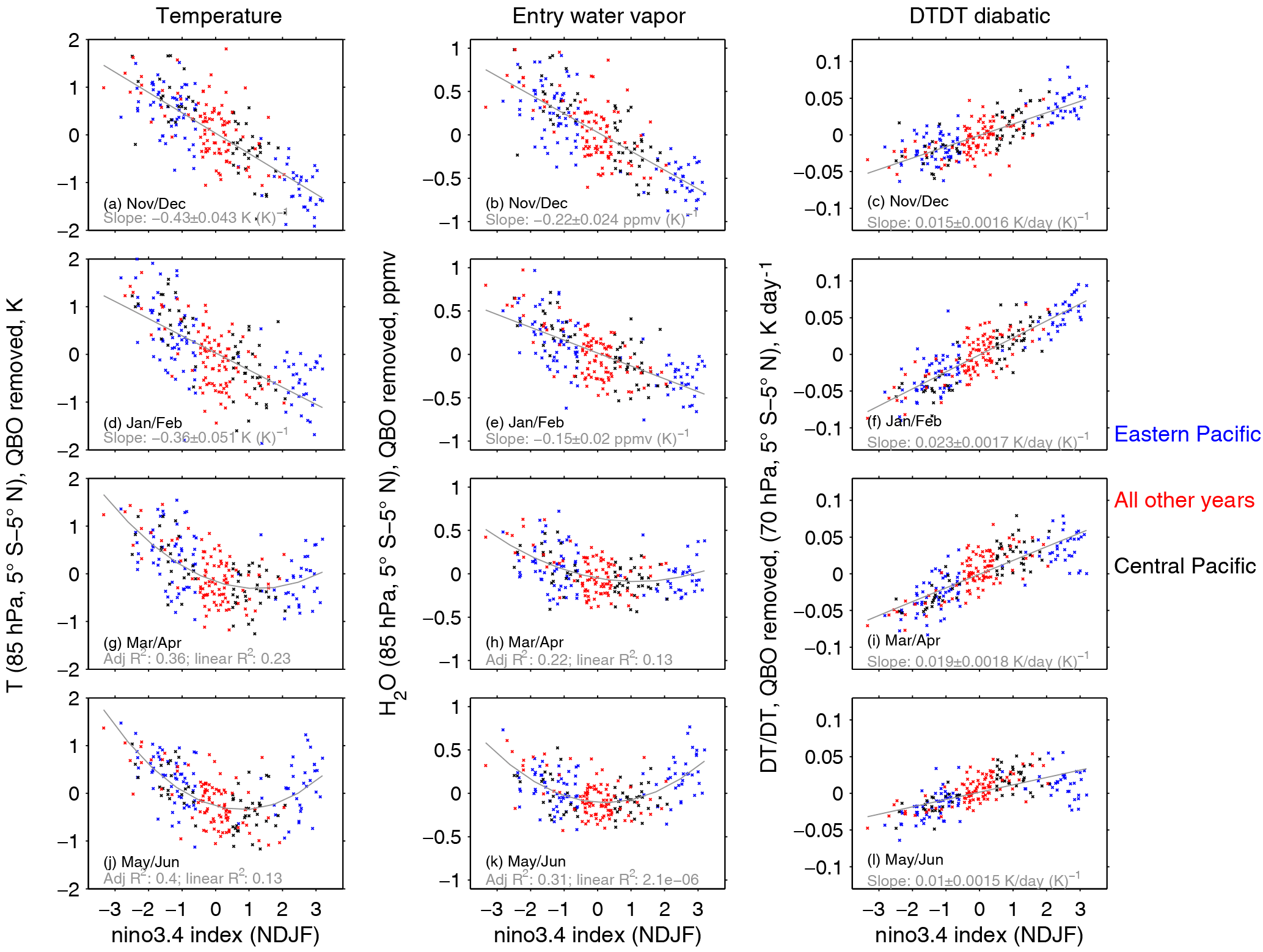
Figure 2 Seasonally resolved anomalies in the tropical lower stratosphere stratified by the Niño-3.4 index in NDJF in the coupled ocean–atmosphere GEOSCCM integration. (a–c) November and December; (d–f) January and February; (g–i) March and April; (j–l) May and June. (a, d, g, j) Temperature at 85 hPa, 5^∘ S–5^∘ N; (b, e, h, k) water vapor at 85 hPa, 5^∘ S–5^∘ N; (c, f, i, l) diabatic heating rate at 70 hPa, 5^∘ S–5^∘ N. For all quantities, the data have been detrended (see Sect. 3) and the component of the variance linearly associated with the QBO at 50 hPa 2 months prior has been regressed out before data are stratified by the Niño-3.4 index (see Sect. 3). Winters categorized as central Pacific ENSO are in black, eastern Pacific ENSO are in blue, and all other years in red. A least-squares best fit is shown in each panel, and the linear slope is indicated when a linear fit is deemed satisfactory (see Sect. 3). When a polynomial fit better describes the dependence on ENSO, we show the R² for a linear fit and adjusted R² for the polynomial fit (see Sect. 3).

4 Linearity of the ENSO effect in the tropical lower stratosphere

We now consider the seasonality and linearity of the ENSO effect in the tropical lower stratosphere. Figure 2 shows the response of temperature, water vapor, and the BDC to ENSO in the coupled ocean–atmosphere run, from November through June. Figure 3 is comparable but for the AGCM integrations, and Fig. 4 is comparable but for MERRA and SWOOSH data. For each panel, the slope and uncertainty of the linear least-squares best fit is indicated if a linear best fit is deemed satisfactory (see the methods section), while the adjusted R² is indicated when a parabolic fit is preferred. Blue markers are used for EP events, and black markers are used for CP events.

We begin with temperature changes in boreal winter. EN leads to strong cooling of the tropical lower stratosphere (Figs. 2a, d, 3a, d), while LN leads to warming relative to the climatology. This temperature response is consistent, to the zeroth order, with the changes in the BDC associated with ENSO: EN leads to an accelerated BDC while LN leads to a decelerated BDC (Figs. 2c, f and 3c, f; see also the Supplement). In November through February, the relationship between ENSO and lower-stratospheric conditions is linear; that is, the impact of EN and LN events of similar strength is equal and opposite. The magnitude of these effects, as quantified by the best-fit line, appears to be slightly weaker in the AGCM ensemble as compared to the coupled ocean–atmosphere runs, and this could be because of differences in the nature of ENSO events or decadal variability. The large spread in values for a given event in Fig. 3 highlights the large amount of internal variability in the tropical lower stratosphere.

Figure 3 As in Fig. 2 but for 42 AGCM GEOSCCM integrations. The ensemble mean response is indicated with a large x, and each ensemble member with a dot.

Figures 2b, e and 3b, e consider changes in water vapor in November through February. In both the AGCM and the coupled ocean–atmosphere simulations EN leads to dehydration. That EN leads to dehydration in boreal winter is in agreement with Calvo et al. (2010), Garfinkel et al. (2013a), and Konopka et al. (2016), who all note the strong seasonal dependence of the effect of EN on stratospheric water vapor.

While the relationship between ENSO and lower-stratospheric conditions is linear in boreal winter, it is nonlinear for both water vapor and temperature in boreal spring (bottom two rows of Figs. 2 and 3). Namely, a parabolic (e.g., H₂0 $\sim a\times {\mathrm{EN}}^{\mathrm{2}}$) fit better describes the relationship between ENSO and water vapor and between ENSO and lower-stratospheric temperature than a linear fit (Figs. 2g, h, j, k and 3g, h, j, k). Hence, strong EN events lead to less cooling than what might have been expected given a linear best fit, and consistent with this, the strongest EN events lead to more moistening than might have been expected based on a linear best-fit line. This is especially evident in Fig. 2h, k, where the strongest EN events lead to spring moistening. The AGCM runs capture this effect as well, as the 1997/1998 EN also leads to moistening (the most extreme EN event in Fig. 3h, k). This effect is explored further in Sect. 5, where we compare the temperature response to the 1997/1998 EN to other EN events.

It does not matter whether the ENSO event is categorized as a CP or EP event, as the red, black, and blue dots all indicate the same relationship between ENSO and water vapor. However, the strongest EN events tend to be EP in both nature and in the coupled ocean integration, and hence the nonlinearity is less detectable for CP events. This difference in strength also explains why the compositing approach of Garfinkel et al. (2013a) to characterizing the impact of EP events and CP events can mislead: the atmospheric response to a composite of EP events may differ from the response to a composite of CP events because the events included in the EP composite are stronger, not because of the specific pattern of the SST anomalies.

Figure 4 As in Figs. 2 and 3 but for the MERRA reanalysis (a, d, g, j and c, f, i, l) and SWOOSH (b, e, h, k).

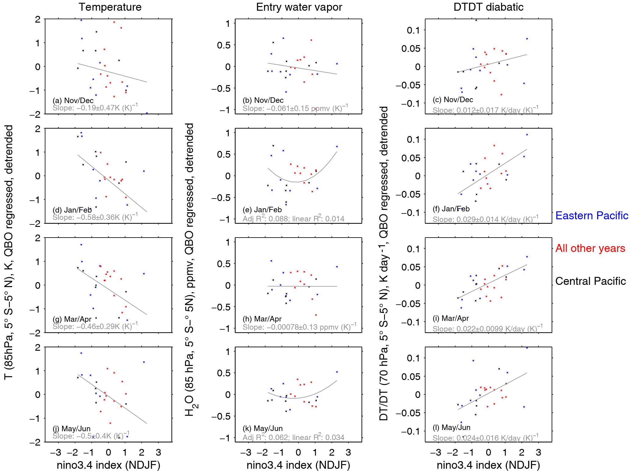
The response to ENSO in GEOSCCM can be used to inform the interpretation of the observed response to ENSO (Fig. 4). EN leads to an accelerated BDC and a colder lower stratosphere in reanalysis data in January and February, and these changes are statistically indistinguishable from the response in GEOSCCM. More importantly, the qualitatively different behavior for the 1997/1998 event as compared to moderate EN events in the model experiments is also evident in observations in March through June, and hence we recommend caution against generalizing from the observed anomalies in the tropical lower stratosphere in 1997/1998 to other, more moderate EN events. However, the relatively short data record limits the confidence with which we can identify nonlinearities in observational and reanalysis data, and none of the linear best-fit slope estimates for SWOOSH water vapor are statistically significant in either winter or spring.

5 Composite analysis of the 1997/1998 event as compared to other events

In order to better understand why strong EN events may affect the boreal spring tropical lower stratosphere differently from weak events, we compare the 1997/1998 event to other EN events in the AGCM GEOSCCM runs. The time evolution of the water vapor anomalies associated with the 1997/1998 event are shown in Fig. 5a, and b shows the water vapor anomalies associated with all other EN events. There is clearly a large difference, with the 1997/1998 event leading to robust moistening peaking at 0.4 ppmv in June while all other events have little effect.

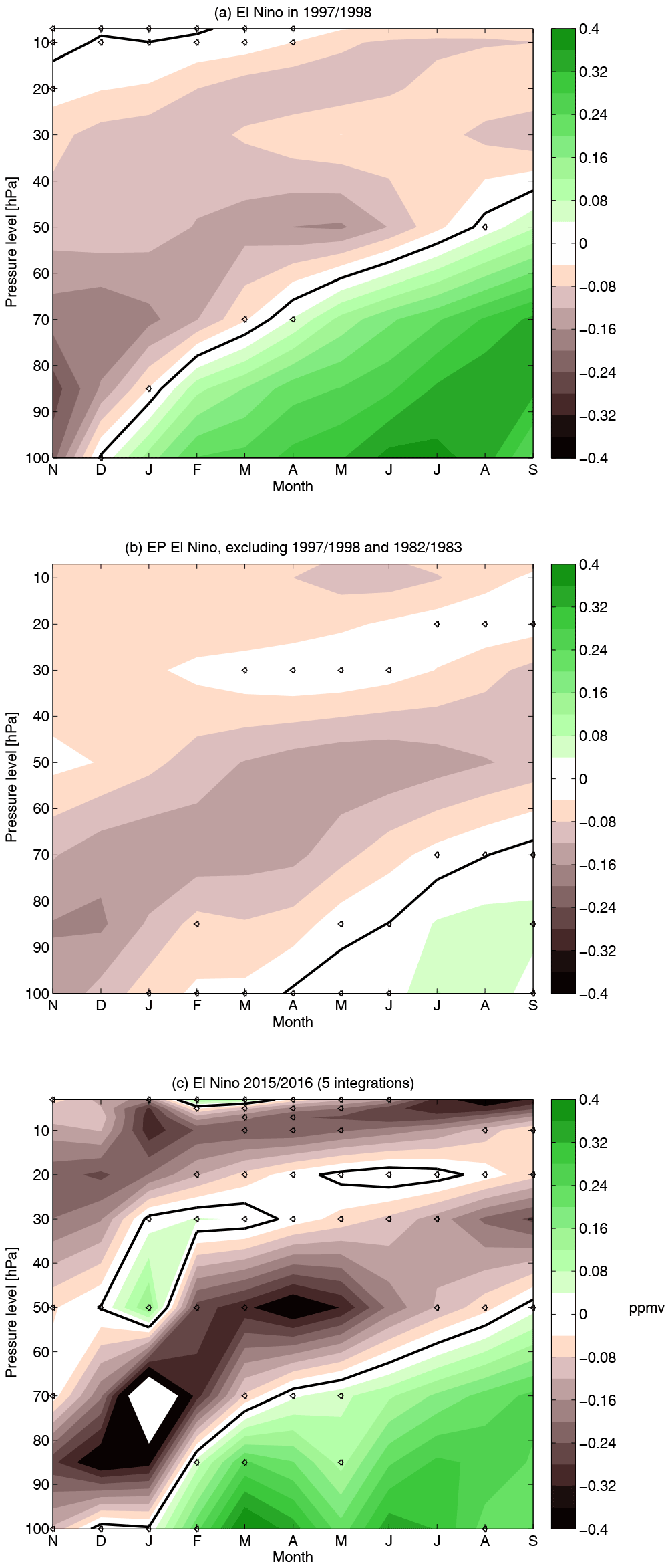
Figure 5 Water vapor anomalies (ppmv) for the 42 AGCM GEOSCCM integrations in (a) 1997/1998; (b) all EPEN events except 1997/1998 and 1982/1983; (c) 2015/2016 in the five integrations that have been extended to the near present. Anomalies that are not significant at the 95 % level are marked by black symbols. The effect of the QBO at 50 hPa and the linear trend have been linearly regressed out of all anomalies before EN composites are formed (see Sect. 3).

Figures 6 and 7 show a map view of changes in temperature at 100 hPa for the 1997/1998 event and for all other EP EN events. The green contour on each panel surrounds the coldest region of the tropics climatologically, while the magenta contour surrounds the coldest region of the tropics during the specific EN composite. In both Figs. 6 and 7 there is relative cooling between 170 and 120^∘ W and relative warming over the warm pool region from November through February (consistent with Yulaeva and Wallace, 1994; Randel et al., 2000; Scherllin-Pirscher et al., 2012), but the longitude of the zero line between warming and cooling differs between the 1997/1998 event and all other EP EN events. Specifically, in the 1997/1998 event in boreal winter, the zero line of temperature anomalies is 30^∘ further east than for the other EP EN events (compare the black zero line in Figs. 6b and 7b), such that during the 1997/1998 event the entirety of the climatological cold point region warms. The net effect of this warming of the climatological cold point region is that the cold point shifts to the east while warming during 1997/1998 (the magenta isotherm is 0.7 K warmer than the green contour in Fig. 6). In contrast, during other EP EN events, roughly half of the climatological cold point region warms while the other half cools, and the net effect is that the coldest region shifts east but does not warm or cool overall for typical EP EN events (the green and magenta isotherms in Fig. 7 correspond to the same temperature). The eastward shift in Figs. 6b and 7a, b is consistent with the shift in the Lagrangian cold point evident in Figs. 8 and 9 of Bonazzola and Haynes (2004) and Fig. 8 of Hasebe and Noguchi (2016). In boreal spring, there is broad-scale warming over most of the equatorial band for the 1997/1998 event (Fig. 6cd), while the temperature anomalies are similar to those in winter for moderate EN events (Fig. 7c, d). A similar effect is seen in the MERRA reanalysis (not shown). The net effect is that in boreal winter and especially spring, the 1997/1998 event led to warming of the cold point and moistening of the stratosphere relative to other EP EN events.

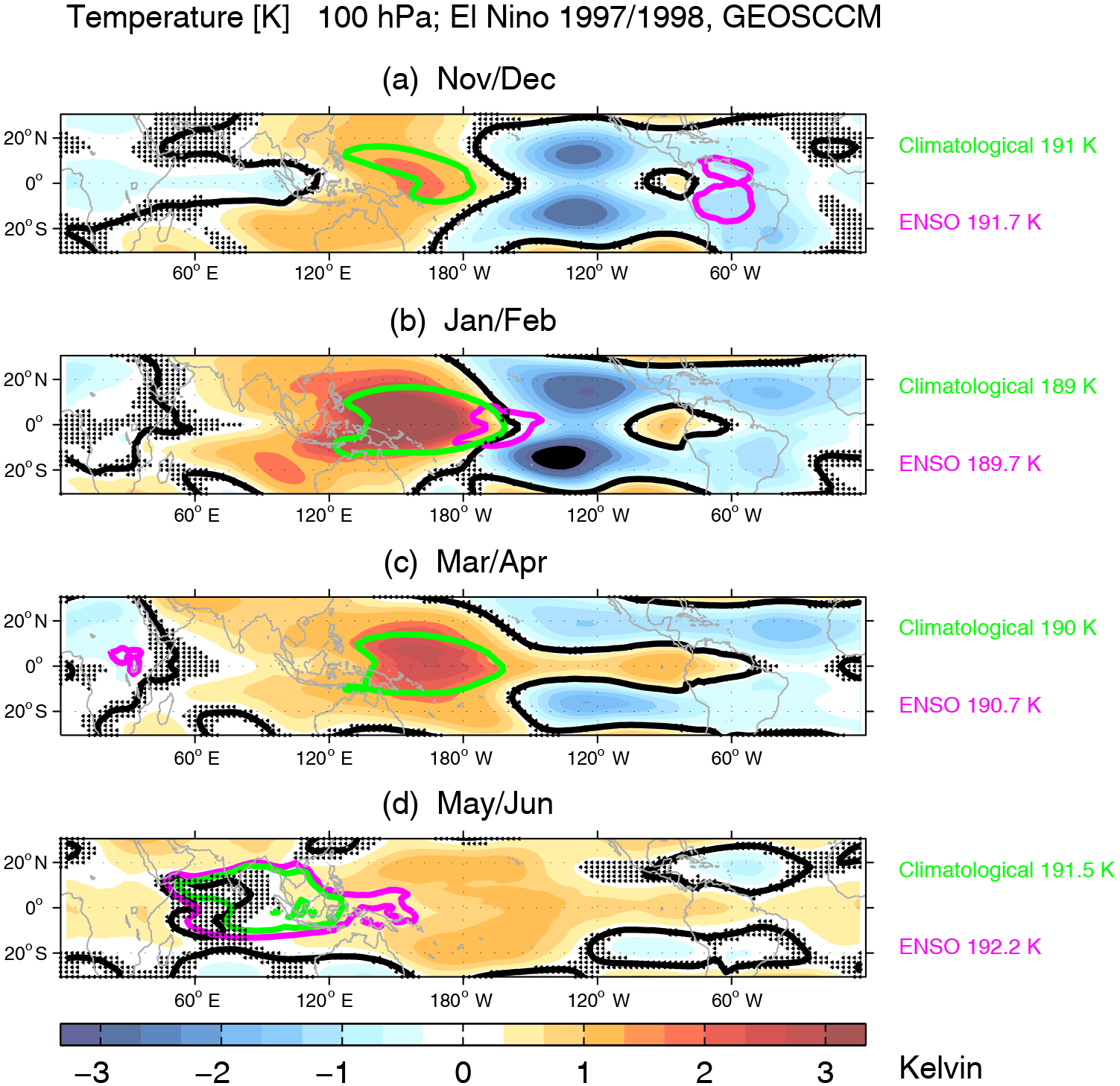
Figure 6 Temperature anomalies (Kelvin) at 100 hPa for 1997/1998 in the GEOSCCM AGCM integrations in November–December (a) through the following May–June (d). Anomalies that are not significant at the 95 % level are marked by black symbols. The green and magenta contours denote specific cold isotherms in the climatology and for this specific composite in order to highlight the location of the cold point. The effect of the QBO at 50 hPa and the linear trend have been linearly regressed out of all anomalies before ENSO composites are formed (see Sect. 3). The contour interval is 1∕3 K.

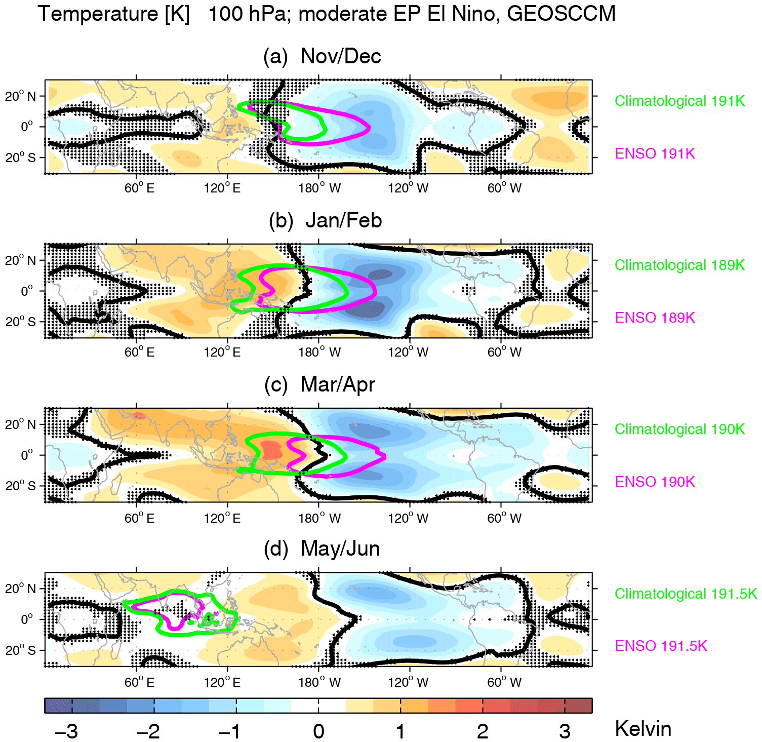
Figure 7 As in Fig. 6 but for all ENSO events except 1982/1983 and 1997/1998 in the GEOSCCM AGCM integrations.

The changes in tropical temperature in GEOSCCM for the 1997/1998 event and for other events are summarized in Fig. 8, which shows the temperature averaged from 5^∘ S to 5^∘ N from 300 to 50 hPa. The overall quadrupole structure is similar to that in Liang et al. (2011) and Garfinkel et al. (2013b), and there is an eastward shift of the cold point region. The model captures the warming pattern in reanalysis (compare Figs. 8 and S1 in the Supplement). Most pertinently, there are clear differences between the changes in 1997/1998 and those in other EN years: the tropospheric warming is more pronounced and widespread in 1997/1998 from March through June. The net effect is that the cold point region warms in 1997/1998 but not in the other EN years.

It is important to emphasize that this nonlinearity in the temperature and water vapor response does not involve stratospheric dynamics. The changes in the BDC appear to be mostly linear in Figs. 2, 3, and 4. The wave driving of the BDC is not the source of the nonlinearity (see the Supplement). Rather, the 1997/1998 event led to exceptional warming throughout the tropopause transition layer and at the cold point as is evident in Fig. 8 and the Supplement, and hence led to enhanced water vapor entering the stratosphere.

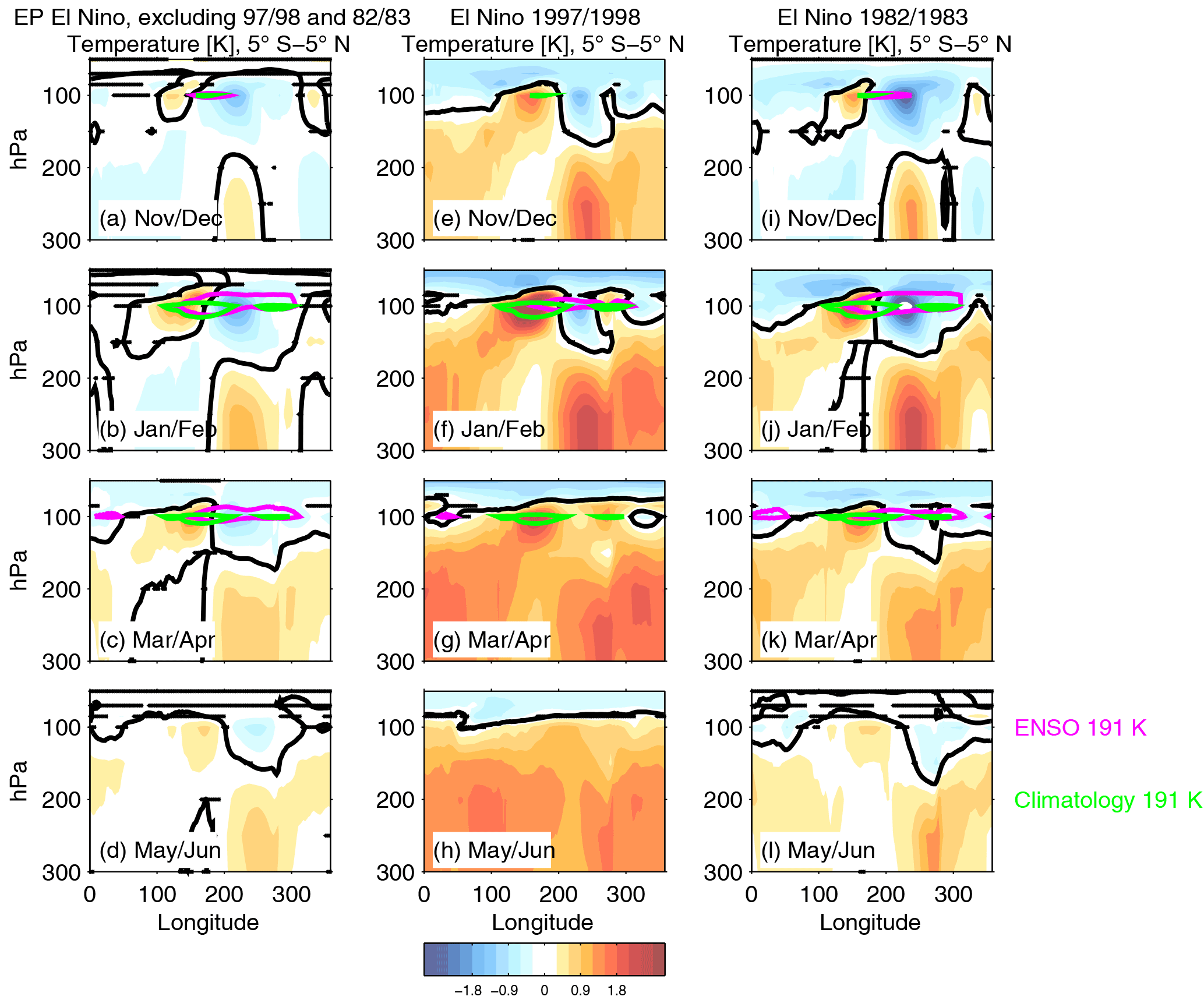
Figure 8 Tropical (5^∘ S–5^∘ N) temperature anomalies (Kelvin) (a–d) for all EP EN events excluding 1997/1998 and 1982/1983, (e–h) 1997/1998, and (i–l) 1982/1983, in the AGCM simulations. Anomalies that are not significant at the 95 % level are marked by black symbols. The green and magenta contours denote specific cold isotherms in the climatology and for this specific composite in order to highlight the location of the cold point. The effect of the QBO at 50 hPa and the linear trend have been linearly regressed out of all anomalies before ENSO composites are formed (see Sect. 3). The contour interval is 0.3 K.

Why was the 1997/1998 EN tropospheric warming so distinct from other events? While this was the strongest EN over the period considered by this paper, the 1982/1983 EN was not much weaker than the 1997/1998 event as measured by the Niño-3.4 index, yet the impact of the 1982/1983 event on water vapor was qualitatively different. Furthermore, the upper-tropospheric warming in the central and eastern Pacific sectors for the 1982/1983 and 1997/1998 events (Fig. 8) is similar. This suggests that the central and eastern Pacific responses cannot explain the difference in stratospheric response. In contrast, these two events differed quite dramatically in the Indian Ocean (and more generally in zonally averaged tropical temperature). The 1997/1998 event led to remarkable impacts in the Indian Ocean: warm anomalies exceeded 2 ^∘C locally over the western Indian Ocean and enhanced convection over Africa was anomalously strong even for EN (Webster et al., 1999; Su et al., 2001). SSTs north of the Equator were anomalously warm throughout 1998 as well (Yu and Rienecker, 2000). The cold point moves toward India over the course of boreal spring (e.g., Bonazzola and Haynes, 2004; Garfinkel et al., 2013a) and thus warming in this area can impact water vapor. This difference in near-surface conditions in the Indo-Pacific and Niño-3.4 regions is quantified in Fig. 1. EN events are followed by warming throughout the Indo-West Pacific (Fig. 1a, c). Conditions during the 1982/1983 event are shown with a red diamond and during the 1997/1998 event with a large red x. Despite largely similar anomalies in the Niño-3.4 region, the 1997/1998 event was characterized by remarkably warm anomalies in the Indo-Pacific that lie in the tail of the warming generated spontaneously in the coupled ocean–atmosphere model.

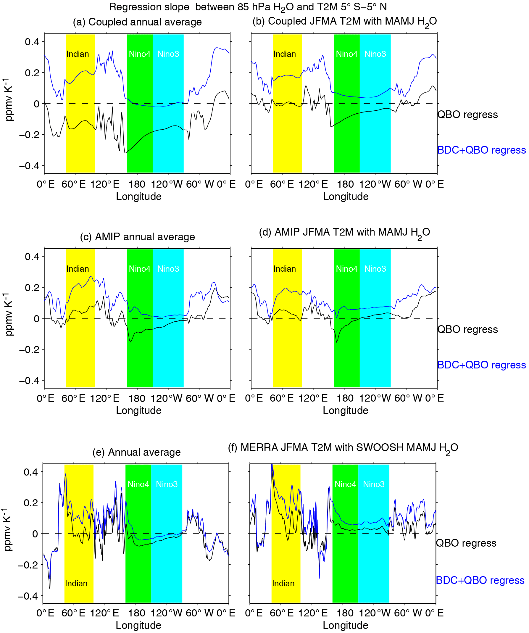
Figure 9 Regression coefficient between tropical (5^∘ S and 5^∘ N) 2 m temperature (T2m) and zonally averaged entry water vapor at 85 hPa in (a–b) the last 240 years of a coupled ocean–atmosphere run, (c–d) the AGCM runs, and (e–f) for SWOOSH water vapor and MERRA 2 m temperatures. The longitude bands corresponding to the Indian Ocean, Niño-3, and Niño-4 regions are in color. The left column is for annual averaged quantities and the right column is for March through June water vapor with T2m 2 months prior. We show resulting regression coefficients after first regressing out the effect of the QBO at 50 hPa from the water vapor anomalies (black) and also after regressing out the effect of the QBO at 50 hPa and the BDC from the water vapor anomalies (blue).

The importance of Indian Ocean SSTs for entry water vapor is quantified in Fig. 9, which shows the regression coefficient between 85 hPa water vapor and 2 m temperatures from 5^∘ S to 5^∘ N at each longitude grid point. We show both the regression coefficient in the annual average with no lag between water vapor and surface temperature and in boreal spring with 2 m temperatures leading water vapor by 2 months (Garfinkel et al., 2013a). The black curve shows the regression after linearly regressing out the BDC and the QBO from the water vapor, and the blue curve the regression after linearly regressing out the QBO from the water vapor.

In the annual average, warmer near-surface temperatures over the central and eastern Pacific lead to dehydration of the stratosphere in all three data sources (black curves in Fig. 9a, c, e), though during boreal spring warming in the eastern Pacific leads to moistening of the stratosphere 2 months later. More importantly however, stratospheric water vapor is most sensitive to variability in the Indian Ocean and western Pacific basins, with warmer temperatures in this region leading to enhanced water vapor in all three data sources in boreal spring (and if the BDC influence on water vapor is regressed out, also in the annual average). While the importance of a large regression coefficient in a given region depends on the magnitude of near-surface temperature variations in that region, results are similar if correlations are examined (not shown).

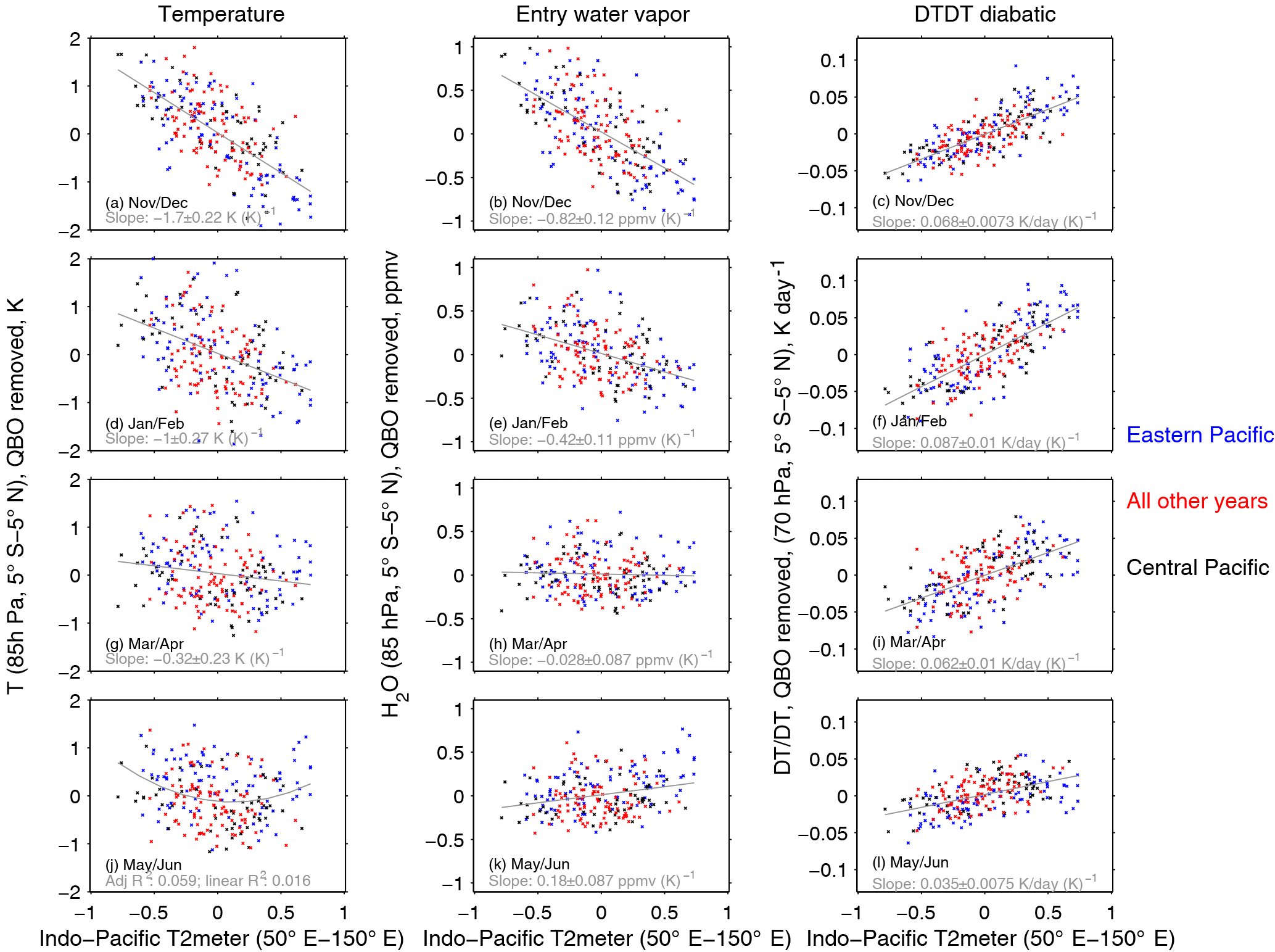
Figure 10 As in Fig. 2 but stratifying years based on 2 m temperature from 50 to 150^∘ E, 5^∘ S–5^∘ N.

Figure 10 demonstrates that the nonlinearity of the boreal spring stratospheric response in temperature and water vapor to EN is due to Indo-West Pacific surface temperatures. It is constructed similarly to Fig. 2, but motivated by Fig. 9 the years are stratified by 2 m temperatures from 50 to 150^∘ E instead of by the Niño-3.4 index. Instead of the pronounced boreal spring nonlinearity evident in Fig. 2, the lower-stratospheric response to Indo-West Pacific surface temperature is linear in all seasons. In November through February a warmer Indo-Pacific leads to impacts similar to those of ENSO (compare top row of Figs. 2 to 10). In March and April, however, a warmer Indo-West Pacific leads to an accelerated BDC and a colder lower stratosphere, but to no robust changes in water vapor. In May and June, a warmer Indo-West Pacific still leads to an accelerated BDC, but despite this accelerated BDC the lower stratosphere moistens. Results are similar for the AGCM integrations (not shown), with the 1997/1998 event leading to lower-stratosphere moistening despite an accelerated BDC.

In summary, an ENSO event that more efficiently warms the mid-troposphere (such as the 1997/1998 event) by modifying SSTs in the Indian Ocean can more efficiently moisten the stratosphere. Strong EN events tend to have a stronger impact on the Indian Ocean than more moderate events (cf. Fig. 1), and hence their impact on the tropical lower stratosphere in the boreal spring and early summer is more pronounced, which ultimately leads to nonlinearity in the connection between EN and the tropical lower stratosphere.

6 Implications for the drop in the early 2000s and the 2015/2016 EN event

It has been suggested that SST changes in the Indo-Pacific contributed to some of the drop in water vapor after the year 2000 (Rosenlof and Reid, 2008; Garfinkel et al., 2013b) via ENSO (Brinkop et al., 2016), and here we consider whether the AGCM simulations simulate a drop. Before proceeding, it is important to mention that the 1997/1998 EN was followed by nearly 3 consecutive years of strong LN conditions – the Niño-3.4 index in the ERSST5 dataset did not drop below −0.5 K until March 2001 – which was then followed by weak EN conditions from 2002 through 2004. As discussed above, strong LN events also lead to moistening of the stratosphere, while weak EN lead to dehydration. The net effect is that ENSO was in a phase that leads to enhanced water vapor during 1998, 1999, and 2000 and in a phase that leads to reduced water vapor from 2002 to 2004. It has already been documented that QBO and BDC variability are key ingredients for the observed drop (Randel et al., 2006; Fueglistaler, 2012; Fueglistaler et al., 2014; Dessler et al., 2014). Note that the QBO phase in these GEOSCCM experiments does not match that observed, and the specific wave events that drove the accelerated BDC in late 2000 are not nudged to occur in these free-running GEOSCCM simulations either. Hence we do not expect to be able to capture the full magnitude of the drop. However, these experiments can be used to quantify the contribution of SSTs to the difference in water vapor between 2002 and 2004 and between 1998 and 2000, and with these caveats duly noted we now proceed.

Figure 11a shows the evolution of anomalous annual averaged entry water vapor between 5^∘ S and 5^∘ N in the AGCM simulations (excluding the simulations that represent the eruption of Mt. Pinatubo), with the brown line showing the mean across all simulations, the black line showing the mean of the five simulations that have been extended through the end of 2016, and thin lines showing the evolution in those five simulations individually. It is evident from the brown line in Fig. 11a that these integrations simulate a pronounced decrease in the early 2000s. If we define the drop as the difference in water vapor between 2002 and 2004 and between 1998 and 2000, the imposed SSTs can account for an ensemble-averaged dehydration of about 0.14 ppmv. Note that we focus on annual averaged entry water vapor, and so the timing of the drop (between 2000 and 2001) is fully consistent with the timing of the observed drop as calculated by Fueglistaler (2012) and Hasebe and Noguchi (2016). The mean value is approximately one-quarter of the total drop (which equals 0.62 ppmv in the deep tropics if we apply the same definition to SWOOSH data, though as shown by Fueglistaler et al. (2013) the different satellite products that underly the SWOOSH data disagree as to the magnitude of the drop.) As discussed above, the rest of the drop is associated with BDC and QBO variability, which these GEOSCCM simulations are not expected to capture. Hence, our GEOSCCM simulations suggest that SST changes contributed to the drop (in agreement with  Rosenlof and Reid, 2008), but were not the major forcing factor, consistent with Garfinkel et al. (2013b), Brinkop et al. (2016), and Ding and Fu (2017). Note that these integrations also simulate a drop after 2011 (Urban et al., 2014; Gilford et al., 2016), suggesting that part of this drop was forced by SSTs as well.

Finally, five of the integrations have been extended to the near present and hence include the 2015/2016 EN event. This event was comparable in strength in the Niño-3.4 region to that in 1997/1998, and while it satisfies the criteria we adopt for an EP event, it was less strongly EP-focused as compared to the 1997/1998 event. We now consider the evolution of water vapor in those integrations in Fig. 11. Note that these simulations are forced with time-varying SSTs and sea ice only.

The model simulates a 0.5 ppmv increase in H₂O in 2016 (annual average) as compared to 2015, approximately 70 % of the observed increase. Hence, the model is clearly capable of capturing the enhanced stratospheric water vapor following strong EN events. The seasonal evolution of the change is shown in Fig. 5c, and the increase in water vapor occurs in March after the EN event has already begun to decay. The moistening in 2016 is comparable to that in 1998 (see Fig. 5ac). Note that the QBO phase in GEOSCCM does not match that observed, and hence we are not surprised that the model misses the observed pronounced drying that occurred in mid-2016 and late-2016 due to the QBO disruption (Tweedy et al., 2017). In summary, strong EN events like those in 2015/2016 and 1997/1998 lead to a pronounced moistening in both GEOSCCM and in nature.

Figure 11 Annual average water anomalies at 85 hPa for the GEOSCCM AGCM experiments. (a) The 85 hPa water vapor between 5^∘ S and 5^∘ N. (b) Cloud ice at 100 hPa between 5^∘ S and 5^∘ N. The thick brown line in (a) indicates the average across all 42 AGCM integrations. A black line indicates the ensemble mean of the five integrations which have been extended to the near present, and color indicates each of these five simulations. (c) Cloud ice anomalies at 85 hPa in December 2015 in the ensemble mean of these five simulations. No detrending has been performed on any of the time series.

7 Conclusions

Tropical lower-stratospheric temperature and water vapor changes have important implications for both stratospheric and tropospheric climate as well as stratospheric ozone chemistry (SPARC-CCMVal, 2010; World Meteorological Organization, 2011, 2014). Hence, it is crucial to understand interannual changes in this region in order to correctly interpret future changes. Analysis of a series of chemistry–climate atmospheric model integrations in two distinct configurations – coupled to an interactive ocean model and forced by historical sea surface temperatures – yielded the following conclusions:

1. The impact of El Niño–Southern Oscillation on temperature and water vapor in this region is nonlinear in boreal spring. While moderate El Niño events lead to cooling in this region, strong El Niño events lead to warming, even as the response of the large-scale Brewer–Dobson circulation appears to scale nearly linearly with El Niño. The tropospheric warming associated with strong El Niño events extends into the tropical tropopause layer and up to the cold point, where it allows for more water vapor to enter the stratosphere. The net effect is that both strong La Niña and strong El Niño events lead to enhanced entry water vapor and stratospheric moistening in boreal spring. Only in boreal winter is the response linear. The source of the spring nonlinearity is the Indo-West Pacific response to El Niño: strong El Niño events lead to warming in this region that subsequently warms the cold point and moistens the tropical lower stratosphere.

2. There is no appreciable difference in the tropical lower-stratospheric response to central Pacific versus eastern Pacific El Niño events, if one controls for the amplitude of the El Niño event. As eastern Pacific El Niño events tend to be stronger, however, the nonlinear effects discussed above are pronounced mainly for events of this type.

3. The very strong El Niño event in 1997/1998 followed by more than 2 consecutive years of La Niña led to enhanced lower-stratospheric water vapor. As this period ended in early 2001, entry water vapor concentrations declined. We quantify this effect using a large ensemble of AGCM simulations with imposed SSTs, and find that the deterministic part of the water vapor drop arising from these imposed SSTs is about one-quarter of that actually observed, in agreement with the recent estimate of Ding and Fu (2017), who used a different model. Hence, it is important to consider SST variability when considering decadal variability in the lower stratosphere, though other forcings were more important for the drop in the early 2000s as only one-quarter of the drop can be directly accounted for by SSTs.

In light of these results, we wish to emphasize that two commonly used methodologies in stratospheric research can lead to misleading conclusions. First, multiple linear regression approaches to attributing stratospheric variability in water vapor and temperature to forcings such as ENSO are problematic, as the stratospheric response to ENSO in water vapor and temperature is nonlinear in the tropical lower stratosphere in boreal spring and early summer. Second, compositing approaches of ENSO into central Pacific and eastern Pacific types can also lead one astray, as central Pacific El Niños are weaker and a naive compositing analysis cannot distinguish whether a difference in response is due to differences in spatial patterns rather than differences in event amplitude. Specifically, Garfinkel et al. (2013a) compared EP EN events including 1997/1998 to all CP EN events. A more meaningful comparison is EP EN events excluding 1997/1998 to all CP EN events, and our GEOSCCM experiments suggest that there is no difference in stratospheric response for such a comparison of composites.

This study leaves several unanswered questions. First, the ENSO amplitude in the ocean model used here for our coupled ocean–atmosphere simulations is too large (Capotondi et al., 2015), and mean state biases are also present (e.g., Figs. 3 and 4 of Li et al., 2016); the results from GEOSCCM presented here need to be confirmed with other models. Second, it is not mechanistically clear how upper-tropospheric warming over the Indo-West Pacific leads to moistening of the stratosphere in boreal spring. However, this effect appears to be consistent with recent suggestions that mid-tropospheric warming can directly lead to a warmer cold point tropopause and wetter stratosphere (Dessler et al., 2013, 2014). Third, and relatedly, we cannot provide a complete explanation of how El Niño modulates stratospheric water vapor. Interannual variability in stratospheric water vapor, particularly that associated with El Niño, depends both on a “sampling effect” (i.e., changes in the residence time in the coldest regions of the tropical tropopause layer) and a “temperature effect” (Bonazzola and Haynes, 2004; Hasebe and Noguchi, 2016; Konopka et al., 2016). These two effects cannot be distinguished in our simulations since the model output necessary to run a Lagrangian trajectory model was not archived. Nonetheless neither is prevented from operating in the simulations and the simulated interannual variability in water vapor will arise from some combination of the two. In addition, direct injection of cloud ice may be important for stratospheric water vapor during El Niño: Avery et al. (2017) find enhanced cloud ice in CALIPSO data in December 2015 during the most recent strong El Niño event. We therefore briefly consider whether the model can capture this effect in Fig. 11b, which shows tropical cloud ice between 5^∘ S and 5^∘ N at 100 hPa. Our GEOSCCM simulations capture a jump in tropical cloud ice at 100 hPa of around 0.5 ppmv associated with this event, in general agreement with CALIPSO data (Avery et al., 2017), and even at 85 hPa cloud ice increases by 0.05 ppm in the zonal mean. The spatial distribution of the change in cloud ice at 85 hPa in December 2015 is shown in Fig. 11c; the pattern of anomalous ice matches that found in CALIPSO data (see Fig. 1 of Avery et al., 2017). While the ice cloud parameterization in this version of GEOSCCM is crude, the qualitative agreement between CALIPSO and GEOSCCM suggests that direct injection of ice may not be an insignificant pathway for stratospheric water vapor during strong El Niño events, and this effect should be explored as models improve. More generally, entry water vapor may be influenced by physical processes that are missing or poorly represented by the current generation of climate models, and hence all results shown here with regards to water vapor should be reevaluated as models improve.

However, the nonlinearity of the lower-stratospheric response in temperature and water vapor to El Niño is robust and appears to depend on large-scale circulation and temperature anomalies, which we expect our model to capture. Hence caution must be exercised when deciding on a methodology for analyzing the tropical stratospheric response to El Niño.