the Creative Commons Attribution 4.0 License.
the Creative Commons Attribution 4.0 License.
 | 05 Mar 2018
Lower tropospheric ozone over India and its linkage to the South Asian monsoon
Lin Zhang
Xiong Liu
Yuanhong Zhao
Jingyuan Shao
Lower tropospheric (surface to 600 hPa) ozone over India poses serious risks to both human health and crops, and potentially affects global ozone distribution through frequent deep convection in tropical regions. Our current understanding of the processes controlling seasonal and long-term variations in lower tropospheric ozone over this region is rather limited due to spatially and temporally sparse observations. Here we present an integrated process analysis of the seasonal cycle, interannual variability, and long-term trends of lower tropospheric ozone over India and its linkage to the South Asian monsoon using the Ozone Monitoring Instrument (OMI) satellite observations for years 2006–2014 interpreted with a global chemical transport model (GEOS-Chem) simulation for 1990–2010. OMI observed lower tropospheric ozone over India averaged for 2006–2010, showing the highest concentrations (54.1 ppbv) in the pre-summer monsoon season (May) and the lowest concentrations (40.5 ppbv) in the summer monsoon season (August). Process analyses in GEOS-Chem show that hot and dry meteorological conditions and active biomass burning together contribute to 5.8 Tg more ozone being produced in the lower troposphere in India in May than January. The onset of the summer monsoon brings ozone-unfavorable meteorological conditions and strong upward transport, which all lead to large decreases in the lower tropospheric ozone burden. Interannually, we find that both OMI and GEOS-Chem indicate strong positive correlations (r=0.55–0.58) between ozone and surface temperature in pre-summer monsoon seasons, with larger correlations found in high NOx emission regions reflecting NOx-limited production conditions. Summer monsoon seasonal mean ozone levels are strongly controlled by monsoon strengths. Lower ozone concentrations are found in stronger monsoon seasons mainly due to less ozone net chemical production. Furthermore, model simulations over 1990–2010 estimate a mean annual trend of 0.19 ± 0.07 (p value < 0.01) ppbv yr−1 in Indian lower tropospheric ozone over this period, which are mainly driven by increases in anthropogenic emissions with a small contribution (about 7 %) from global methane concentration increases.
- Article
(9698 KB) - Full-text XML
-
Supplement
(5291 KB) - BibTeX
- EndNote


Ozone in the lower troposphere is a harmful air pollutant for both humans and the ecosystem (Monks et al., 2015), and plays a central role in atmospheric chemistry as the major source of hydroxyl radicals (OH) (Jacob, 2000). It is also a short-lived greenhouse gas with a global mean radiative forcing of 0.40 (0.20–0.60) W m−2 since the preindustrial era (Myhre et al., 2013; Stevenson et al., 2013). Tropospheric ozone is produced by sunlight-driven photochemical oxidation of carbon monoxide (CO) and hydrocarbons in the presence of nitrogen oxides (NOx ≡ NO + NO2). These ozone precursors are released not only from anthropogenic sources such as industry and transportation, but also from a number of climate-sensitive natural sources such as lightning, biomass burning, and biogenic emissions. It is also transported from the stratosphere (about 550 Tg yr−1 or 10 % of chemical production in the troposphere) (Stohl et al., 2003; Stevenson et al., 2006). Tropospheric ozone burden (present-day 337 ± 23 Tg) has enhanced 43 % since the preindustrial era due to rapid industrialization (Young et al., 2013). Zhang et al. (2016) recently revealed that increases in the tropospheric ozone burden over the past 30 years were dominated by the equatorward redistribution of anthropogenic emissions to developing regions such as East and South Asia, increasing the interest in ozone pollution over those regions.
Unlike developed regions such as Europe and eastern US, where anthropogenic emission reductions have led to surface ozone levels flatten or decrease since 1990s (Parrish et al., 2012; Cooper et al., 2012; Oltmans et al., 2013; Strode et al., 2015; Lin et al., 2017), developing countries such as China and India have been experiencing anthropogenic emission rises and ozone enhancements (Xu et al., 2008; Cooper et al., 2014; Sun et al., 2016; Wang et al., 2017). Recent studies have shown that NOx emissions in China have been decreasing since 2012 due to stringent air pollution controls (Krotkov et al., 2016; Liu et al., 2017). However, air quality in India is continuously deteriorating as indicated by increasing NO2 columns observed by satellite (Krotkov et al., 2016; Geddes et al., 2016), and may become worse in the near future considering projected trends in population and the associated anthropogenic emissions (Ghude et al., 2016). Exposure to ozone pollution in India is estimated to have caused 12 000 premature deaths in 2011 due to chronic obstructive pulmonary disease (Ghude et al., 2016), and up to a 36 % loss of wheat and other crop productions (Ramanathan et al., 2014; Sinha et al., 2015). In addition, frequent deep convection in tropical Asia allows the uplifted pollutants to influence global ozone distribution (Lelieveld et al., 2001; Sahu et al., 2006; Beig and Brasseur, 2006; Park et al., 2007; Lawrence and Lelieveld, 2010; Srivastava et al., 2012a; Lal et al., 2013). A better understanding of the processes controlling lower tropospheric ozone over India thus becomes important to address its local and global environmental effects.
Distinct seasonal transitions in prevailing wind and rainfall associated with the monsoon circulation result in unique ozone variations in South and East Asia. Winter monsoon prevails in October to March and brings dry and cool weather conditions. With the onset of South Asian (East Asian) summer monsoon in May, stronger westerlies (southerlies) bring marine air from Arabian Sea (western Pacific) to the Indian subcontinent (East Asia), leading to significant enhancements of cloud fractions and rainfall (Wang and LinHo, 2002; Ding and Chan, 2005). Decreases of tropospheric ozone with the summer monsoon in South and East Asia have been reported from surface (Lal et al., 2000; Naja and Lal, 2002; Naja et al., 2003; Beig et al., 2007; Reddy et al., 2008; Wang et al., 2009; Kumar et al., 2010; Ding et al., 2013; Hou et al., 2015), ozonesonde (Zhou et al., 2013; Lal et al., 2014; Ojha et al., 2014; Sahu et al., 2014), aircraft measurements (Bhattacharjee et al., 2015; Ding et al., 2008; Srivastava et al., 2015; Ojha et al., 2016), and satellite observations (Liu et al., 2009; Dufour et al., 2010; Safieddine et al., 2016). A number of modeling studies attribute the summertime ozone minimum over India to transport of clean marine air (Lal et al., 2014; Sahu et al., 2014) or reduced ozone photochemical production (Roy et al., 2008; Kumar et al., 2012). This seasonality is in contrast to that at mid-latitudes where surface ozone levels are usually higher in spring and summer due to stronger stratosphere-to-troposphere transport and photochemistry (Parrish et al., 2013; Cooper et al., 2014).
Most of the abovementioned studies used individual ground-based observations or regional chemistry models to study seasonal or short-term interannual (up to 5 years) variability of tropospheric ozone in India. Long-term ground-based ozone observations are extremely scarce in South Asia (Cooper et al., 2014). We also lack a comprehensive analysis of the spatiotemporal distribution of lower tropospheric ozone at a domestic scale in India. In particular, key processes that influence the tropospheric ozone budget over India have not been analyzed and quantified. In this study, we present an integrated analysis of the processes controlling lower tropospheric (surface to 600 hPa) ozone concentrations over the terrestrial land of India and their linkage to the South Asian monsoon. Satellite observations from the Ozone Monitoring Instrument (OMI) over 2006–2014 and simulations with the GEOS-Chem chemical transport model (CTM) for 1990–2010 are used to analyze the spatial, seasonal, and interannual variability of lower tropospheric ozone pollution over India, before and during the South Asian summer monsoon. We will further examine the potential drivers of long-term trends in lower tropospheric ozone over India.
2.1 OMI satellite observations
The OMI instrument is onboard the NASA Earth Observing System (EOS) Aura satellite launched in July 2004 with an ascending equator crossing time of ∼ 13:45 LT (local time) (Schoeberl et al., 2006). OMI is a nadir-viewing instrument that measures backscattered solar radiation in the 0.27–0.5 µm wavelength range with a spectral resolution of 0.42–0.63 nm (Levelt et al., 2006). Its nadir footprint has a spatial resolution of 13 × 24 km2 with near-daily global coverage achieved by a wide view field of 114∘ and a 2600 km wide swath.
We use the OMI PROFOZ ozone profile retrievals developed by Liu et al. (2010) based on the optimal estimation method (Rodgers, 2000). Details of the PROFOZ product have been given in Liu et al. (2010) and Kim et al. (2013), and were recently comprehensively validated by Huang et al. (2017, 2018). This OMI ozone profile algorithm retrieves partial ozone columns for 24 layers with about 2.5 km thickness for each layer. Here we grid the monthly mean OMI data to the 2∘ × 2.5∘ horizontal resolution with focus on the spatial and temporal distributions of Indian lower tropospheric ozone concentrations for the period of 2006–2014. Comparisons of model simulations with OMI retrievals need to consider OMI a priori profiles and averaging kernel matrices as described in Zhang et al. (2010). OMI a priori profiles are from the monthly ozone profile climatology of McPeters et al. (2007). The degrees of freedom for signals (sum of the diagonal elements of averaging kernel matrices) for OMI ozone retrievals are typically 0.3–0.5 in the lower troposphere over India. Previous evaluations of the OMI retrievals with ozonesonde measurements have shown a clear improvement over the a priori in the lower troposphere of the tropics (30∘ S–30∘ N), and the mean retrieval biases in the tropics are less than 6 % with little seasonality (Huang et al., 2017).
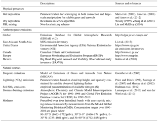
Table 1A summary of physical processes, anthropogenic and natural emissions used in GEOS-Chem.
2.2 GEOS-Chem simulations
We use the GEOS-Chem global CTM (v10-01; http://www.geos-chem.org) in this study. The model includes a detailed mechanism of ozone–NOx–VOC–aerosol tropospheric chemistry (Bey et al., 2001; Park et al., 2004; Mao et al., 2010, 2013) using the chemical kinetics recommended by Jet Propulsion Laboratory (JPL) and International Union of Pure and Applied Chemistry (IUPAC) (Sander et al., 2011; IUPAC, 2013), and photolysis rates calculated by the Fast-JX scheme (Bian and Prather, 2002). Stratospheric ozone chemistry is represented by the linearized ozone parameterization (LINOZ) (McLinden et al., 2000), and other stratospheric species are simulated using monthly averaged production and loss rates archived from the Global Modeling Initiative (GMI) model (Murray et al., 2013). Physical processes such as deposition and planetary boundary layer (PBL) mixing schemes are summarized in Table 1. The model has been applied in a number of studies on global and regional tropospheric ozone (Wang et al., 2013; Fiore et al., 2014; Zhang et al., 2014; Lou et al., 2015; Yan et al., 2016; Zhao et al., 2017). A recent model evaluation with global tropospheric ozone datasets shows that GEOS-Chem (v10-01) provides an improved ozone simulation relative to previous model versions (e.g., v8-01 in Zhang et al., 2010) with no significant seasonal and latitudinal biases (Hu et al., 2017).
The model is driven by the Modern Era Retrospective-analysis for Research and Application (MERRA) assimilated meteorological fields (Rienecker et al., 2011). For input to GEOS-Chem, we downgrade the MERRA data to 2.5∘ longitude × 2∘ latitude and 47 vertical layers (extending from surface to 0.01 hPa) from the raw resolution of 0.667∘ longitude × 0.5∘ latitude and 72 layers. Emissions in the model are processed using the Harvard-NASA Emission Component (HEMCO) (Keller et al., 2014). Year-specific anthropogenic emissions are from the Emissions Database for Global Atmospheric Research (EDGAR v4.2 for emissions over 1990–2008, 2008 emissions are used for simulation afterwards), overwritten with regional emission inventories as summarized in Table 1. Asian anthropogenic emissions are from the MIX emission inventory (Li et al., 2017).
Climate-sensitive natural ozone emissions such as biogenic non-methane volatile organic compounds (NMVOCs) emissions, lightning NOx emissions, and soil NOx emissions are implemented in GEOS-Chem as summarized in Table 1. For the biomass burning emissions, we combine the Atmospheric Chemistry and Climate Model Intercomparison Project (ACCIMP) (Lamarque et al., 2010) for 1990–1996 and the Global Fire Emission Database version 3 (GFED3) (van der Werf et al., 2010) for 1997–2010. Comparison of GFED3 and ACCMIP biomass burning CO emissions for their overlapping years (1997–2000) suggests that ACCMIP is 30 % higher. Here we reduce the 1990–1996 ACCMIP emissions by 30 % to reconcile the two inventories, although this may lead to underestimates of biomass burning emission contributions for the period. We find that biomass burning emissions of CO over India (2.6 Tg a−1 (per annum) for 2006–2010) are relatively small compared with anthropogenic emissions (61.9 Tg a−1). As atmospheric methane has a relatively long lifetime (about 9 years), its concentrations are prescribed in GEOS-Chem using year-specific measured concentrations from the NOAA Global Monitoring Division (GMD) (see Table 1).
We conduct a standard simulation (BASE) with year-specific assimilated meteorology and anthropogenic emissions from 1990 to 2010 with the initial conditions generated by a 2-year spin-up simulation. We also conduct sensitivity simulations by fixing one of the sources at the 1990 conditions, including anthropogenic emissions (FEMIS), global methane concentrations (FCH4), and biomass burning emissions (FBIOB) as summarized in Table 2. Differences between the standard simulation and the sensitivity simulations are then used to estimate influences of interannual changes in the specific source on tropospheric ozone concentrations over India. All simulations are conducted for 1990–2010 as constrained by the availability of MERRA meteorology and emissions.
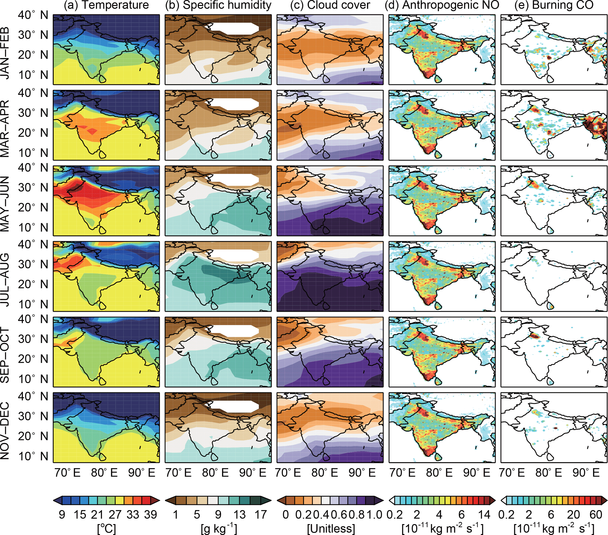
Figure 1Spatial distributions of bimonthly mean (a) surface temperature, (b) 850 hPa specific humidity, (c) cloud cover, (d) anthropogenic NO emissions, and (e) biomass burning CO emissions averaged for 2006–2010.
2.3 Ozone budgets diagnosed in GEOS-Chem
We analyze processes affecting lower tropospheric ozone budgets in each model grid including ozone chemical production and loss, horizontal and vertical transport, and dry deposition. These processes are diagnosed at every hour and averaged to monthly mean. Net productions are calculated as the differences between ozone chemical production and loss rates. Horizontal transport for each grid is calculated by horizontal fluxes from or to adjacent grids. Here we define transport from west to east or from south to north as positive values. Vertical transport is estimated as the flux at the top of the lower troposphere (600 hPa in this study) with positive values representing downward transport. The GEOS-Chem model also includes cloud chemistry (e.g., formation of sulfate aerosol via aqueous-phase reactions with ozone and H2O2) and wet deposition of soluble gases. The two processes have small effects on ozone directly due to its low solubility and thus are not diagnosed here.
3.1 Variations of meteorology and emissions
Variations in tropospheric ozone are subject to changes in precursor emissions and meteorology conditions such as local temperature and transport pattern. Displayed in Figs. 1 and 2 are the spatial and seasonal variations in MERRA meteorological variables (surface temperature, 850 hPa specific humidity (SPHU), and cloud cover), as well as anthropogenic NO emissions, and biomass burning CO emissions over India averaged for the 5-year period (2006–2010). Meteorological conditions in India have distinct seasonal variations associated with the monsoon onset and retreat. Temperature increases from winter (January) to late spring (May) with increasing solar radiation. The onset of the summer monsoon in late May brings moist air from oceans and drives strong air convergence and uplift over India, which lead to cloudy conditions, large decreases in surface temperature (about 8 ∘C from May to August), and enhancements in SPHU (5 g kg−1) (Figs. 1 and 2a). Surface temperature and SPHU become relatively stable with the retreat of the summer monsoon in September, and then both decrease in winter when the winter monsoon brings cold and dry air.
Table 2Configuration of the GEOS-Chem simulations. “V” indicates that specific inputs vary interannually in the simulation, and “1990” denotes that the inputs are fixed to 1990 conditions.
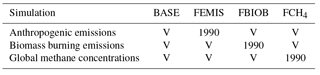
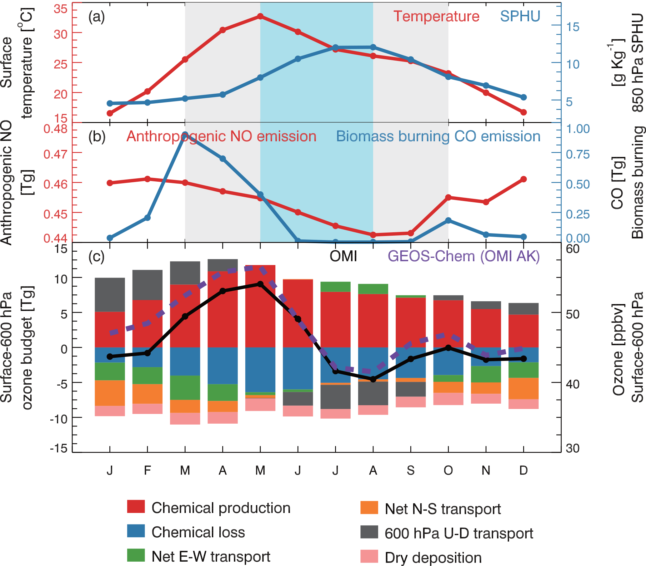
Figure 2Monthly mean (averaged for 2006–2010) (a) surface temperature (red) and 850 hPa averaged specific humidity (SPHU, blue); (b) anthropogenic NO emissions (red) and biomass burning CO emissions (blue); and (c) lower tropospheric ozone (averaged for surface to 600 hPa, in unit of ppbv) from OMI satellite observations (black) and GEOS-Chem model simulations with OMI averaging kernel matrices and a priori profiles applied (dashed purple). The shading in (a, b) represents pre-summer, summer, and post-summer South Asian monsoon periods. Colored bars in (c) show processes that affect lower tropospheric ozone budget over the Indian land diagnosed in GEOS-Chem simulations. Upward (U) and downward (D) vertical transport fluxes are calculated at 600 hPa. Horizontal transport from west (W) to east (E) and from south (S) to north (N), and downward vertical transport are defined as positive values.
Figures 1 and 2b also show anthropogenic NO emissions of 5.44 Tg a−1 (per annum) in India, with emissions in winter (December, January, and February) 3.7 % higher than summer (June, July, and August) due to more active residential heating. Anthropogenic CO and NMVOC emissions over India are 61.9 and 15.5 Tg a−1, respectively, with similar seasonal variations as anthropogenic NO emissions (Fig. S1 in the Supplement). Anthropogenic emissions are higher over northern India including the Indo-Gangetic Plain (IGP, extending from the plain of the Indus River to the plains of the Ganges River) and southern India, consistent with the distribution of population density (Beig and Brasseur, 2006; Kumar et al., 2012). Biomass burning emissions in Southeast Asia are active in March and April (Fig. 1e) and account for 62 % of the annual biomass burning CO emissions in India (Fig. 2b). These emissions are likely due to open burnings during post-harvesting seasons as agricultural field clearance (Venkataraman et al., 2006; Sinha et al., 2014). Hot and dry air conditions in March and April also likely enhance wildfire frequency and strength (Westerling et al., 2006; Jaffe et al., 2008; Lu et al., 2016).
Model calculated biogenic isoprene emissions in India are 39.8 Tg a−1, with a strong seasonality peaking in May and June (Fig. S1 in the Supplement). Previous studies have shown that the ratio of NOx emissions to CO and NMVOCs emissions over India is relatively small compared to other regions at northern mid-latitudes (Lelieveld et al., 2001; Li et al., 2017). Here we also examine the model simulated H2O2 ∕ HNO3 concentration ratios, which have been used as an indicator of ozone production chemical regime (Sillman et al., 1997; Zhang et al., 2016). We find that the H2O2 ∕ HNO3 ratios in the Indian lower troposphere range from 1.0 to 5.0 for all four seasons, higher than those in eastern China and the eastern US (Fig. S2 in the Supplement). This indicates strong NOx-limited conditions for ozone chemical production over India, consistent with previous studies (Kumar et al., 2012; Sharma et al., 2016).
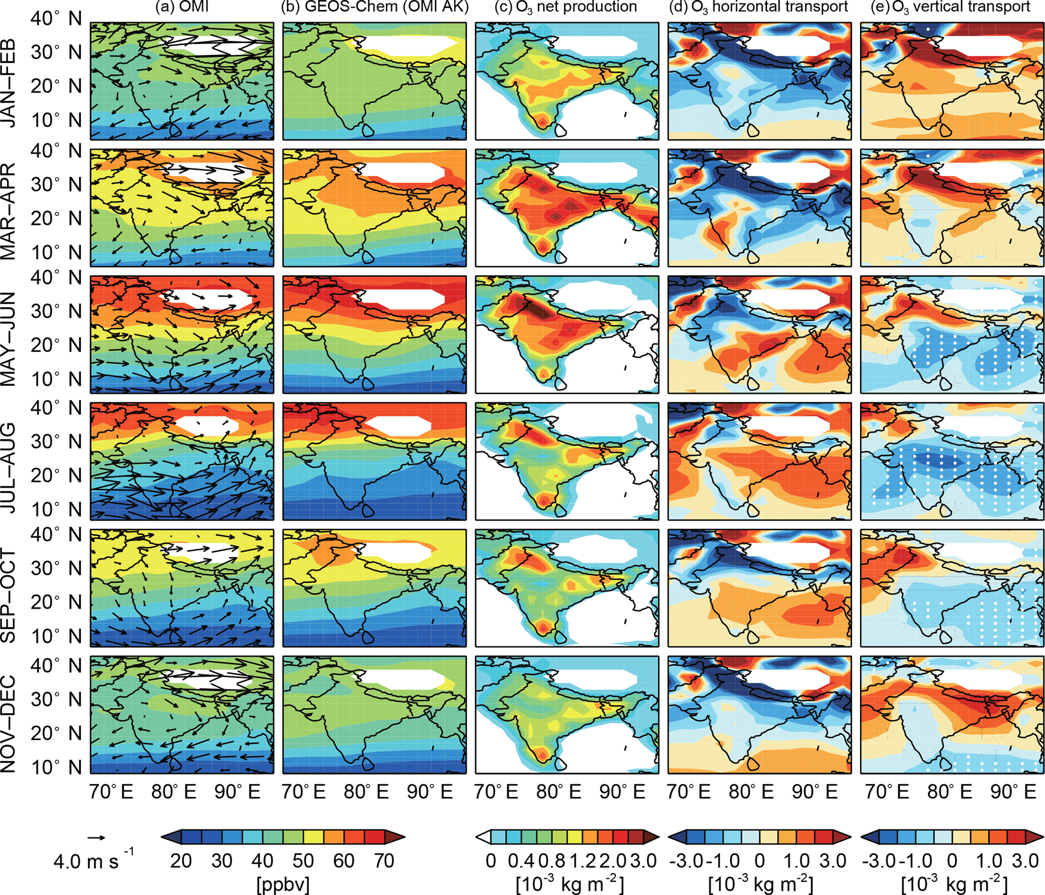
Figure 3Spatial distributions of bimonthly mean lower tropospheric ozone from (a) OMI satellite observations and (b) GEOS-Chem model results (with OMI averaging kernel matrices and a priori profiles applied). Also shown are changes in lower tropospheric ozone burden contributed by (c) net chemical production, (d) net horizontal transport, and (e) vertical transport flux at 600 hPa. All values are averaged for 2006–2010. Wind patterns are overlaid in (a). White dots in (e) denote model grid cells where mean absolute vertical velocities at 600 hPa exceed 5 mm s−1.
3.2 Variations in the pre-summer monsoon season
Figure 2c shows OMI observed and GEOS-Chem model simulated seasonal variations of lower tropospheric ozone concentrations averaged over India and over the 5-year (2006–2010) period. Figure 3 shows their spatial distributions. Model results are applied with OMI averaging kernel matrices and a priori profiles. OMI shows an annual mean lower tropospheric ozone concentration of 45.9 ppbv over India with a maximum (54.1 ppbv) in the pre-summer monsoon season and a minimum (40.5 ppbv) in July–August when the summer monsoon reaches its strongest stage for the year. A similar seasonal cycle of lower tropospheric ozone was found in the Tropospheric Emission Spectrometer (TES) observations (Kumar et al., 2012). Spatially, observed ozone concentrations are higher in northern India and IGP regions than southern regions, consistent with reported surface measurements (Lal et al., 2000; Naja and Lal, 2002; Beig et al., 2007; Reddy et al., 2008; Ojha et al., 2012; Kumar et al., 2012). While model results are about 2 ppbv (4.4 %) higher annually with the largest overestimate occurring in January–May, they generally capture the seasonal and spatial variations of OMI observed lower tropospheric ozone concentrations (r=0.81–0.97 for the spatial variations of OMI observations vs. model results). Comparison of GEOS-Chem surface ozone concentrations for the year 2010 with measurements at six Indian surface sites reported by Sharma et al. (2016) also shows consistent seasonal variations but with positive biases of about 8 ppbv (Fig. S3 in the Supplement; 43.5 ± 7.4 ppbv in the model vs. 35.0 ± 8.4 ppbv in measurements). Similar model overestimates over India are reported in Kumar et al. (2012) using the WRF-Chem and MOZART models, and are likely due to uncertainties in NOx emissions and the coarse model resolution.
Figures 2c and 3 also identify the processes affecting lower tropospheric ozone burden over India. Here we separate our analysis into to four time periods: pre-summer monsoon seasons (March–April), summer monsoon seasons (May–August), post-summer monsoon seasons (August–October), and wintertime (November–following March). In March and April, the mean lower tropospheric ozone concentration over India increases by 9.8 ppbv from the wintertime which can be explained by significant enhancements of ozone production (from 5.1 Tg in January to 10.9 Tg in April) and net production (from 2.9 to 5.0 Tg month−1). As anthropogenic emissions slightly decrease from winter, ozone production enhancements are more likely associated with ozone-favorable weather conditions such as stronger solar radiation and increasing temperature. These changes not only enhance ozone photochemistry efficiencies in the presence of NOx (Jacob and Winner, 2009; Doherty et al., 2013; Pusede et al., 2015), but also increase natural emissions such as biogenic NMVOCs and soil NOx emissions. Biogenic isoprene emissions over India increase from 1.8 Tg month−1 in winter to 5.2 Tg month−1 in the pre-summer monsoon season. The soil NO emissions also increase from 0.08 to 0.21 Tg month−1 (Fig. S1 in the Supplement). Additional ozone enhancements are due to intense biomass burning emissions. Strong ozone production is seen in central eastern India in the pre-summer monsoon season (Fig. 3c) associated with biomass burning regions (Fig. 1e).
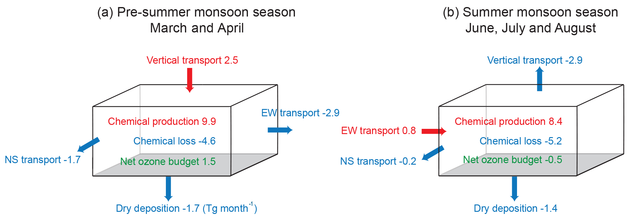
Figure 4Schematic diagram of the lower-tropospheric ozone budget integrated over the Indian terrestrial land in the pre-summer monsoon season (March and April) and in the summer monsoon season (June, July, and August). Values are in unit of Tg month−1.
Horizontal transport (both west–east and north–south transport) decreases Indian lower tropospheric ozone in March–April (Fig. 2c). As shown in Fig. 3a, an anticyclonic wind pattern that dominates the Indian subcontinent during January–April. Prevailing northeastern winds in northern India efficiently transport the ozone-rich air downwind, and circulate into southern India, resulting in a deficient budget in northern India but a positive one in southern India (Figs. 3d and S4 in the Supplement). This low tropospheric transport pattern implies that southern India would likely suffer ozone pollution transported from the ozone-rich northern India in winter and pre-monsoon seasons. Vertical transport at 600 hPa has a positive contribution (2.5 Tg month−1) to the lower tropospheric ozone budget over India in March–April, partly due to the offset from downward import over northern India and upward export over southern India (Fig. 3e). Northern India with higher elevation is likely subject to more stratospheric ozone influences in the period as evidenced by ozonesonde observations and modeling studies (Kumar et al., 2010; Ojha et al., 2014, 2017), while southern India is usually characterized by strong air uplift through convection.
3.3 Variations in the summer monsoon season
The monthly mean lower tropospheric ozone concentration over India decreases from 54 ppbv in May to the seasonal minimum of 40.5 ppbv in August. We find that ozone decrease starts earlier in southern India than in northern India. It can be seen from Fig. 3a that ozone concentrations in the south are higher in March–April than May–June, while ozone in the north reaches its annual maximum in May–June. These patterns can be explained by the temporal differences in the arrival of the summer monsoon (Kumar et al., 2012).
The onset of the South Asian summer monsoon in late May is usually signaled by the prevailing westerly winds from the Arabian Sea to the Bay of Bengal (Wang and Ho, 2002; Gadgil, 2003), leading to cloudy and rainy weather conditions over the Indian subcontinent. Rainfalls efficiently remove ozone precursors as shown from satellite observation of NO2 column (Kumar et al., 2012). Weak solar radiation and low temperature are not favorable for ozone photochemical formation. In addition, water vapor from marine air serves as a chemical loss of ozone at low NOx conditions (Jacob et al., 2000). The onset of the summer monsoon also brings strong air convergence and uplift as indicated by the large-scale air upward velocity in May–August (Fig. 3e). Biomass burning emissions are negligible in the summer monsoon season, and anthropogenic emissions also reach their annual minimum. These changes combined lead to declines in monthly ozone chemical production by 4.2 Tg (from 11.8 Tg in May to 7.6 Tg in August) as integrated over the Indian terrestrial land.
Comparable to chemical production, changes in vertical transport also show a large contribution to the decline of lower tropospheric ozone over India in the summer monsoon season. The monthly vertical transport flux at 600 hPa integrated over India is near zero in May, and reaches −3.3 Tg in August, offsetting the net ozone production in this month (2.9 Tg). Strong vertical convection with the 600 hPa uplift velocity greater than 5 mm s−1 in July–August effectively uplifts ozone pollution from the lower troposphere to the upper troposphere which means it can then be carried by the easterly jet to other parts of the world, such as the Mediterranean (Park et al., 2007; Lawrence and Lelieveld, 2010; Lal et al., 2013), affecting the global tropospheric ozone distribution. We find that horizontal transport from the ocean can lower ozone over northwestern India, especially in May and June when the summer monsoon arrives, consistent with previous observations (Srivastava et al., 2012b; Lal et al., 2014). Horizontal transport also enhances lower tropospheric ozone concentrations in eastern India and the Bay of Bengal (Fig. 3d). The overall contribution of horizontal transport to the Indian lower tropospheric ozone budget is thus relatively small in July–August (0.91 Tg month−1) relative to vertical export (Fig. 2c). Figure 4 summarizes changes in the lower tropospheric ozone budgets over India in the pre-summer monsoon season (March–April) and the summer monsoon season (June–July–August). One can see that decreases in the Indian lower tropospheric ozone in the summer monsoon season are mainly associated with the reduction in ozone net chemical production and strengthening upward transport. Dry deposition of ozone to India shows a weak seasonal variation (1.5 ± 0.15 Tg month−1; Figs. 2c and S1d in the Supplement).
3.4 Variations in the post-monsoon season and wintertime
Lower tropospheric ozone concentrations over India increase slightly in September and reach a second peak in October, associated with increases in precursor emissions and decreases in upward transport. With the southward movement of solar radiation and the summer monsoon retreat, both surface temperature and lower tropospheric specific humidity show decreasing patterns (Fig. 1), leading to reductions in ozone chemical loss. In addition, the retreat of the summer monsoon reduces air uplift over the Indian subcontinent (Fig. 3e), which allows 2.8 Tg more ozone to remain in the Indian lower troposphere in October compared to September (Fig. 2c).
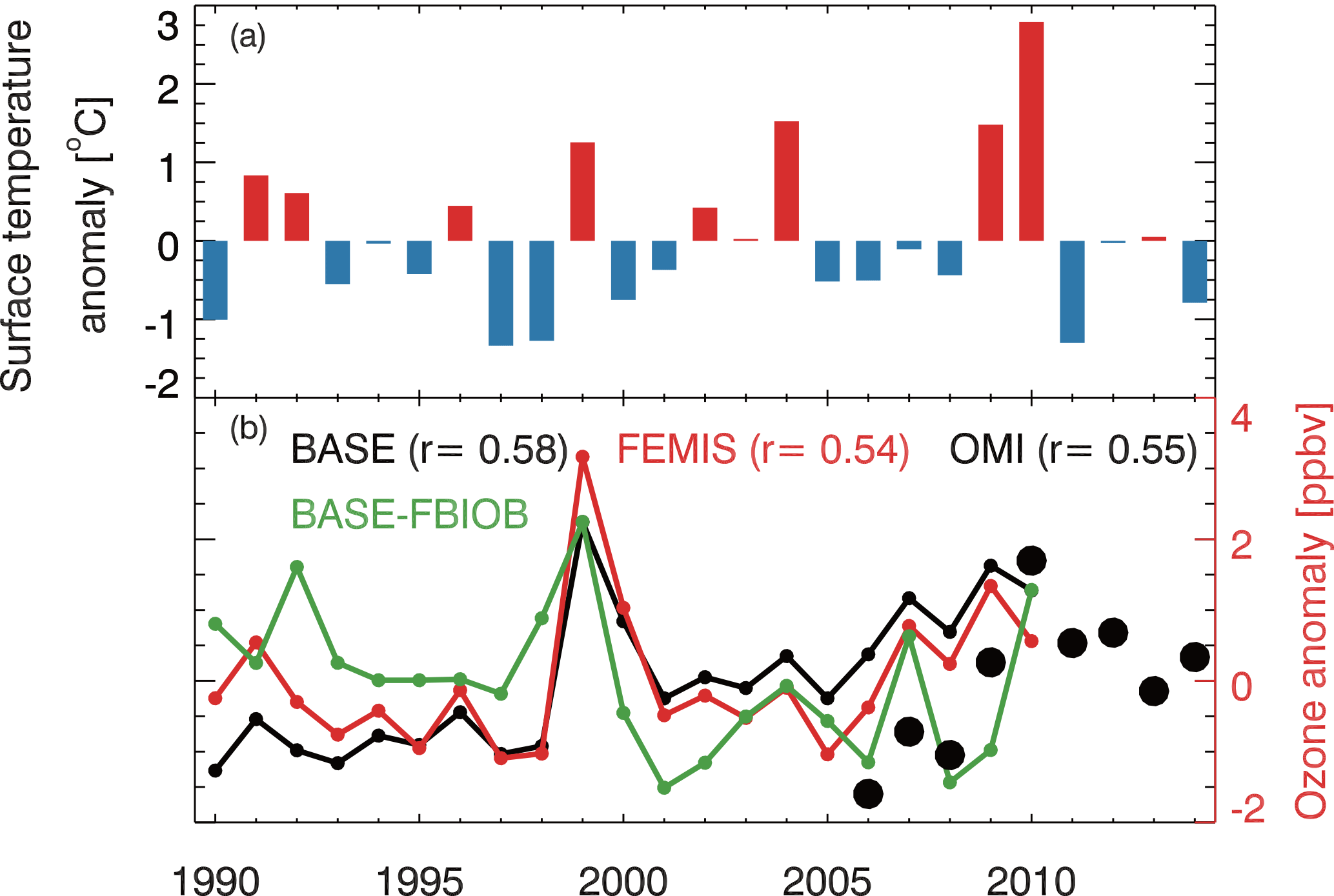
Figure 5Time series of mean (a) surface temperature and (b) lower tropospheric ozone anomaly averaged for pre-summer monsoon seasons over the Indian terrestrial land. OMI observed ozone anomalies are shown by black circles, and model results from the BASE and FEMIS simulations are shown by black and red lines, respectively. The green line shows the ozone anomaly contributed by biomass burning emissions. Interannual correlation coefficients (r) between surface temperature and ozone (number of regional averages n=9 for observations and 21 for model results) are shown in the inset.
From November to the following March, ozone production in the Indian lower troposphere reaches its annual minimum (4.7 Tg month−1 in December) due to low temperature conditions. Horizontal wind patterns are similar to those in the pre-summer monsoon season with a large negative contribution (−5.2 Tg month−1 in November–February) to the Indian lower tropospheric ozone budget. The emergence of the winter monsoon leads to large-scale air subsidence over northern India, with a total import flux of 2.9 Tg month−1 in November–February. The low ozone net production and strong horizontal export result in relatively low ozone levels in wintertime (43.6 ppbv in the lower troposphere). It should be noted that some observational studies reported the highest surface ozone concentrations at several urban or semi-urban sites in southern India (e.g., Ahmedabad, 23∘ N, 73∘ E; Pune, 18∘ N, 74∘ E; Trivandrum, 8∘ N, 77∘ E) in wintertime instead of the pre-summer monsoon season likely due to high local precursor emissions (Beig et al., 2007; David and Nair, 2011; Kumar et al., 2012; Lal et al., 2014; Sahu et al., 2014). Ozonesonde observations at the Ahmedabad and Hyderabad airports (Lal et al., 2014; Sahu et al., 2014) indicate that ozone concentrations in the free troposphere (near 5 km) are higher in the pre-summer monsoon season than winter, consistent with OMI observations in our study.
4.1 Correlation with surface temperature in pre-summer monsoon seasons
We now analyze interannual variability of lower tropospheric ozone in India with focus on pre-summer monsoon seasons when concentrations are highest and summer monsoon seasons when concentrations are subject to monsoon variability. As discussed in Sect. 3.2, tropospheric ozone concentrations in the pre-summer monsoon season are largely controlled by ozone production enhancements due to ozone-favorable weather conditions such as high temperature, and are likely amplified by biomass burning emissions. We also find strong interannual correlations between surface temperature and lower tropospheric ozone concentrations over India. Figure 5 shows that 9-year (2006–2014) time series of OMI observations have a positive interannual correlation (r=0.55) with MERRA surface temperature averaged over India in pre-summer monsoon seasons. GEOS-Chem model results (the BASE simulation) for the period of 1990–2010 captured this positive correlation (r=0.58), and the correlation persists when both variables are detrended (r=0.50).
Figure 6 shows the spatial distribution of correlation coefficients between the lower tropospheric ozone concentration (OMI vs. GEOS-Chem) and surface temperature in pre-summer monsoon seasons. Stronger correlations (r≈0.8) are found in northern India (e.g., the IGP regions) and southern India where NOx emissions are high. The dependence of the ozone–temperature relationship on NOx emission levels is consistent with previous studies reflecting higher ozone formation potential over high NOx regions (Jacob and Winner, 2009; Doherty et al., 2013; Pusede et al., 2015). We examine the overall sensitivity of the ozone–temperature correlation in India to emissions. As shown in Fig. 5, the sensitivity simulation with fixed anthropogenic emissions (FEMIS) shows a slightly lower correlation (r=0.54). It indicates that despite the dependence of ozone–temperature correlations on NOx emission levels regionally, as shown above, the mean correlation over India shows a positive effect of temperature on ozone chemical production, which can be driven by solar radiation affecting both temperature and ozone production rates, as well as the sensitivities of natural sources to temperature as discuss above.
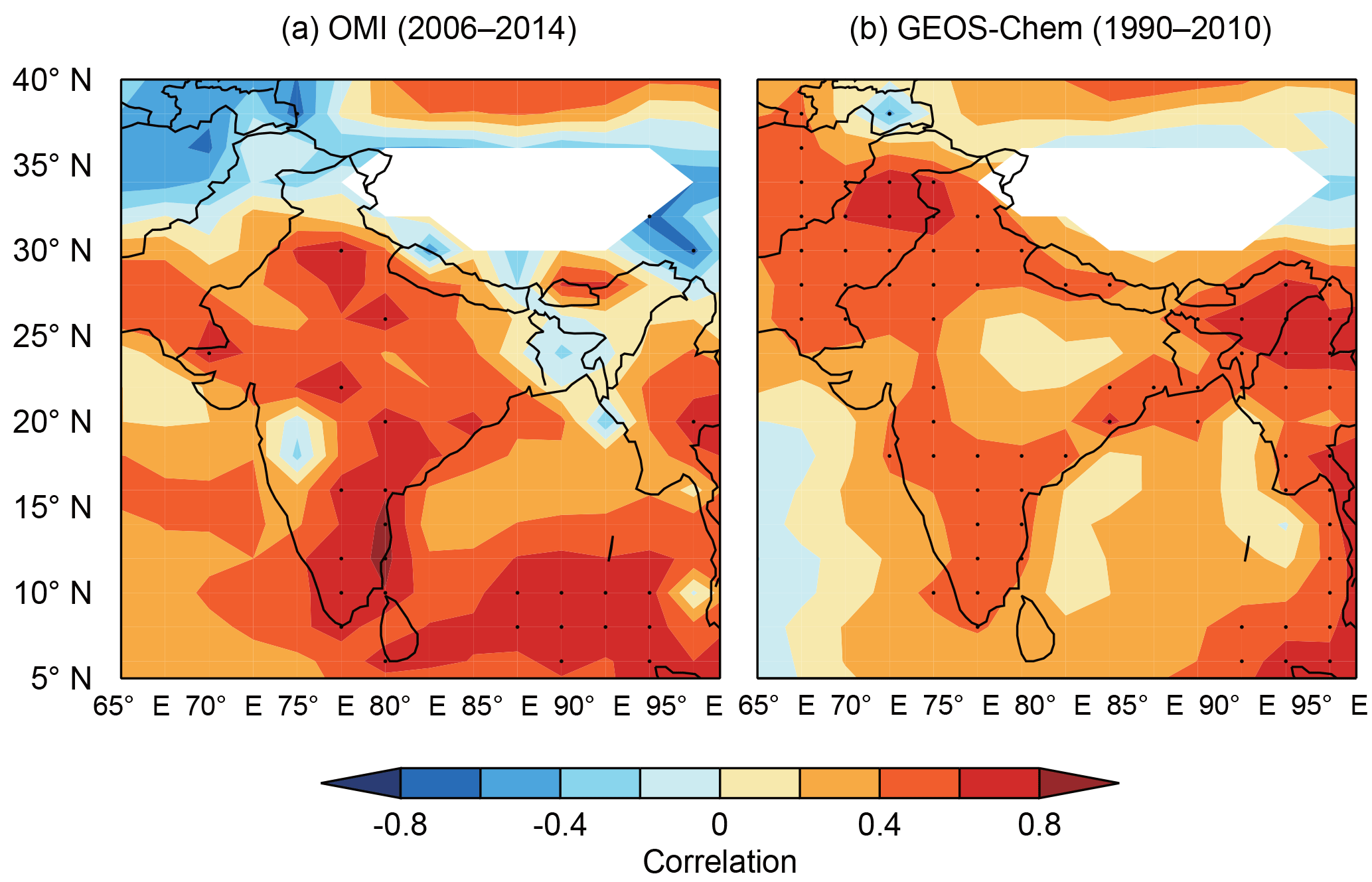
Figure 6Spatial distribution of correlation coefficients between seasonal mean surface temperature and lower tropospheric ozone in pre-summer monsoon seasons calculated for each model grid from (a) OMI satellite observations for 2006–2014 and (b) the GEOS-Chem BASE simulation for 1990–2010. Black dots denote statistical significance (p value < 0.05).
We also calculate the interannual variability contributed by biomass burning emissions as ozone differences between the BASE simulation and the FBIOB simulation. Biomass burning emissions have a large interannual variability with CO emissions ranging from 0.97 to 4.7 Tg over 1990–2010 (Fig. S5 in the Supplement). As can be seen from Fig. 5, the ozone interannual variability contributed by biomass burning emissions is weakly correlated with the BASE lower tropospheric ozone (r=0.29). However, they are important in high ozone and high temperature years. In years such as 1999 and 2010, biomass burning caused 1.5–2.2 ppbv higher ozone, enhancing the variability of lower tropospheric ozone. This eventuality has also been noted in the western US (Jaffe et al., 2008; Lu et al., 2016) as high temperature conditions favored both biomass burning emissions and ozone production, and thus amplified lower tropospheric ozone concentrations.
4.2 Impact of monsoon strength in summer monsoon seasons
We have also shown above that lower tropospheric ozone concentrations over India vary relative to the onset and retreat of the South Asian summer monsoon. The interannual variability of lower tropospheric ozone over India in the summer monsoon seasons (May–August) can then be affected by the strength of the South Asian summer monsoon. To quantify this relationship, we calculate the monsoon strength using the monsoon index proposed by Li and Zeng (2002) which has been applied to quantify impacts of the East Asian monsoon on air pollution over China (Zhu et al., 2012; Yang et al., 2014). The monsoon index is first calculated for each model grid (δ(i,j)) in the Northern Hemisphere in the month m and year y as
where represents monthly mean wind speed from the MERRA dataset, and and are climatological (1990–2010 in our study) monthly wind speed in January and July, respectively. The norm of a given variable A is defined as
where S represents the spatial area of a model grid cell. Details for the calculation of ∥A∥ are given in Li and Zeng (2002) and Zhu et al. (2012). In this study, we then average δ(i,j) over the region of 35–90∘ E, 5–35∘ N (Fig. S2 in the Supplement) at 850 hPa and over May–August to represent the South Asian summer monsoon index (SASMI).
Figure 7 shows the time series of SASMI anomalies relative to the 1990–2014 climatology, and their correlations with OMI observed and model simulated lower tropospheric ozone concentration anomalies over India for the summer monsoon seasons. Positive and negative SASMI values represent strong and weak summer monsoons, respectively. We find no significant trend in the South Asian summer monsoon strength over 1990–2014. Interannual variations of Indian regional mean lower tropospheric ozone concentrations are significantly negative correlated with the SASMI, as can be seen for both OMI observations (, 2006–2014, n=9) and GEOS-Chem BASE results (, 1990–2010, n=21). Removing interannual changes in anthropogenic emissions (FEMIS) results in a stronger correlation of −0.72, reflecting the dominant role of monsoon strength on the interannual variability of Indian lower tropospheric ozone in summer monsoon seasons. We find that the correlations between SASMI and simulated ozone are even stronger at the surface level ( for BASE and for FEMIS; figure not shown).
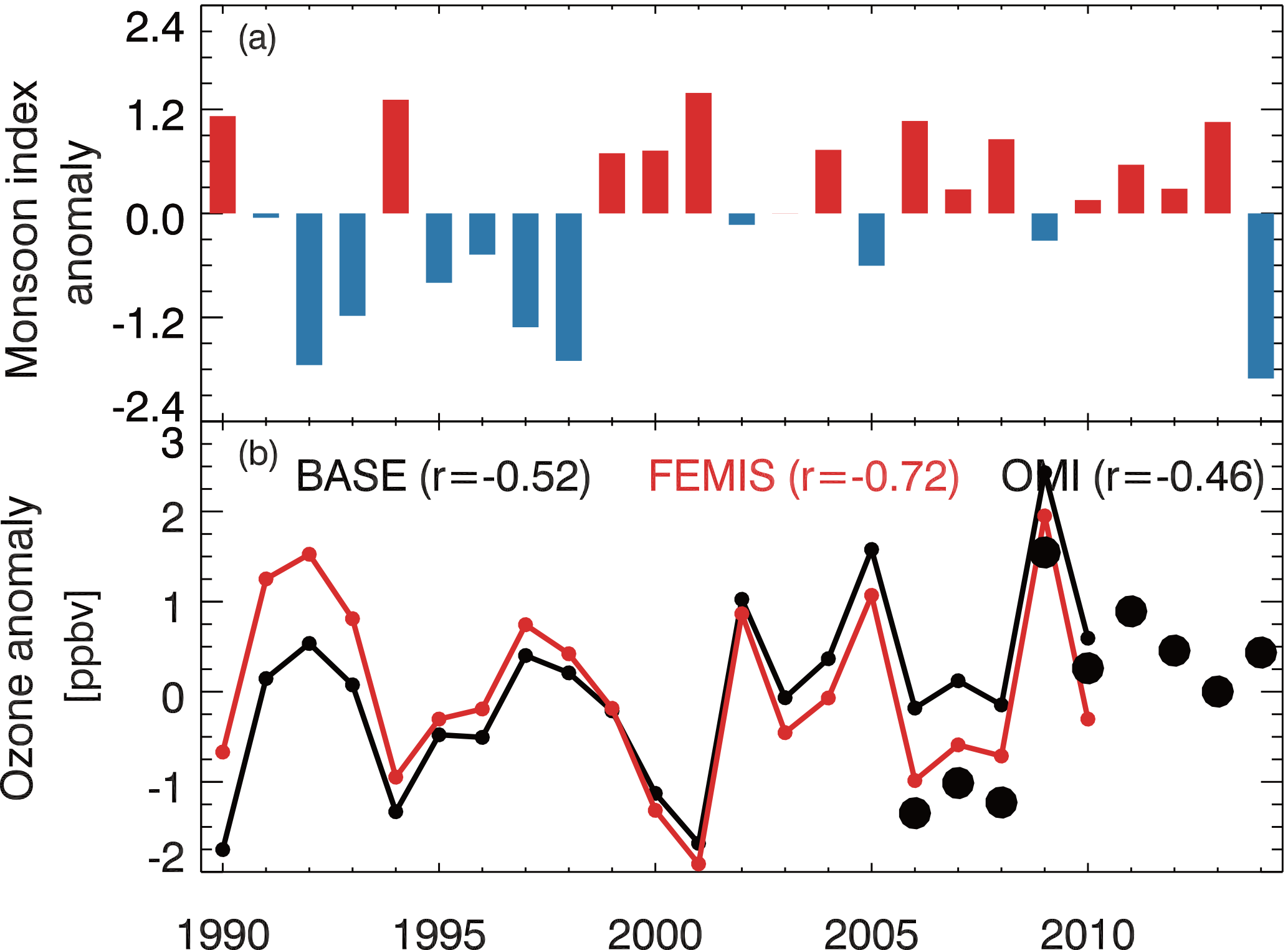
Figure 7Time series of (a) South Asian summer monsoon index and (b) lower tropospheric ozone averaged over India in summer monsoon seasons. Values are anomalies over 1990–2010. OMI observed ozone anomalies are shown by black circles, and model results from the BASE and the FEMIS simulation are shown by black and red lines, respectively. Interannual correlation coefficients with the monsoon index are shown inset.
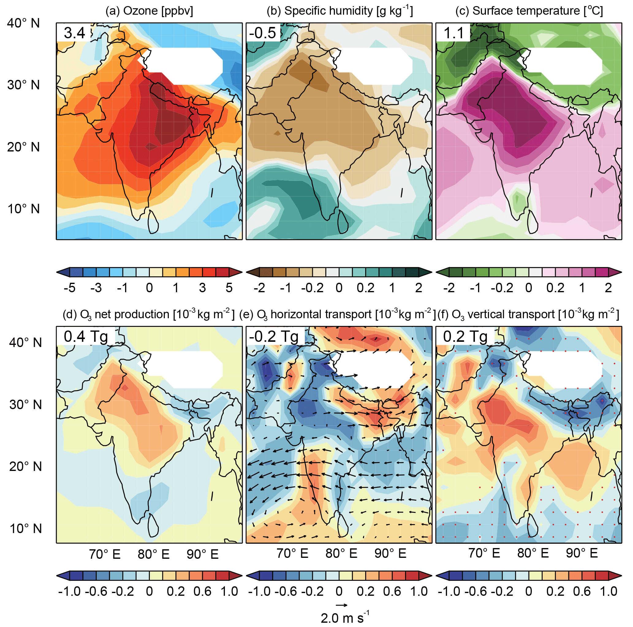
Figure 8Differences in May–August monthly mean (a) lower tropospheric ozone concentration, (b) surface temperature, (c) 850 hPa specific humidity, (d) lower tropospheric net ozone production, (e) lower tropospheric net horizontal transport with wind vectors overlaid, and (f) vertical transport at 600 hPa between the lowest and highest SASMI conditions. Values are calculated using averages of the five lowest SASMI years minus averages of the five highest SASMI years. Values inset are averages (a–c) or totals (d–f) over the Indian terrestrial land. Red dots in (f) denote regions with stronger air uplift in weak compared to strong summer monsoon years.
Yang et al. (2014) previously found positive correlations between the East Asian summer monsoon strengths and surface ozone concentrations over mainland China. They attributed higher surface ozone in stronger summer monsoon years to a smaller outflow of ozone to the East China Sea. Our results show the opposite response from lower tropospheric ozone to summer monsoon strengths over India. To understand the negative correlations, we illustrate in Fig. 8 the differences in meteorological variables, lower tropospheric ozone concentrations, and relevant processes between the weakest and strongest monsoon years (represented by averages over 5 years with the lowest and the highest SASMI over 1990–2010, respectively). We focus on model results from the FEMIS simulation to exclude the influence of interannual changes in anthropogenic emissions. We find that lower tropospheric ozone concentrations averaged over India are 3.4 ppbv higher in weak summer monsoon years than those in strong monsoon years. Weak summer monsoon conditions show higher surface temperature (1.1 ∘C), drier air (−0.5 g kg−1), and lower cloud cover over India, together accounting for a higher ozone net production of 0.4 Tg month−1 than the strong summer monsoon conditions (Fig. 8). In addition, weaker convergence and convection in weak summer monsoon years can cause the total upward ozone flux to be 0.2 Tg month−1 smaller, but this is closely offset by stronger horizontal outflows. Together, we find that the difference in ozone net production is the key factor explaining the difference in the lower tropospheric ozone burden over India between strong and weak summer monsoon years.
As for the long-term trend in the Indian lower tropospheric ozone, the 9-year OMI observations appear to be too short to provide a long-term trend estimate. As can be seen from Figs. 5 and 7, OMI observed mean Indian lower tropospheric ozone concentrations over 2006–2014 show large positive trends of 0.42 ± 0.38 ppbv yr−1 (mean ± 95 % confidence level, p value = 0.03) for the pre-summer monsoon seasons and 0.58 ± 0.71 ppbv yr−1 (p value = 0.09) for the summer monsoon seasons. However, these 9-year trends are mainly driven by the low values from the years 2006 to 2008. It should be acknowledged that the OMI dataset are likely influenced by the OMI row anomaly that potentially results in overestimates in ozone trends over the tropics (Huang et al., 2017).
Here we analyze the long-term trends over the period 1990–2010 simulated by the GEOS-Chem model. Figure 9 shows the spatial distribution of simulated lower tropospheric ozone trends for the annual average, as well as for averages in pre-summer monsoon seasons and summer monsoon seasons. Annually, the Indian lower tropospheric ozone is increasing at a statistically significant rate of 0.19 ± 0.07 (p value < 0.01) ppbv yr−1. Larger ozone trends (0.27 ± 0.12 ppbv yr−1, p value < 0.01) are shown in pre-summer monsoon seasons than those in summer monsoon seasons (0.16 ± 0.14 ppbv yr−1).
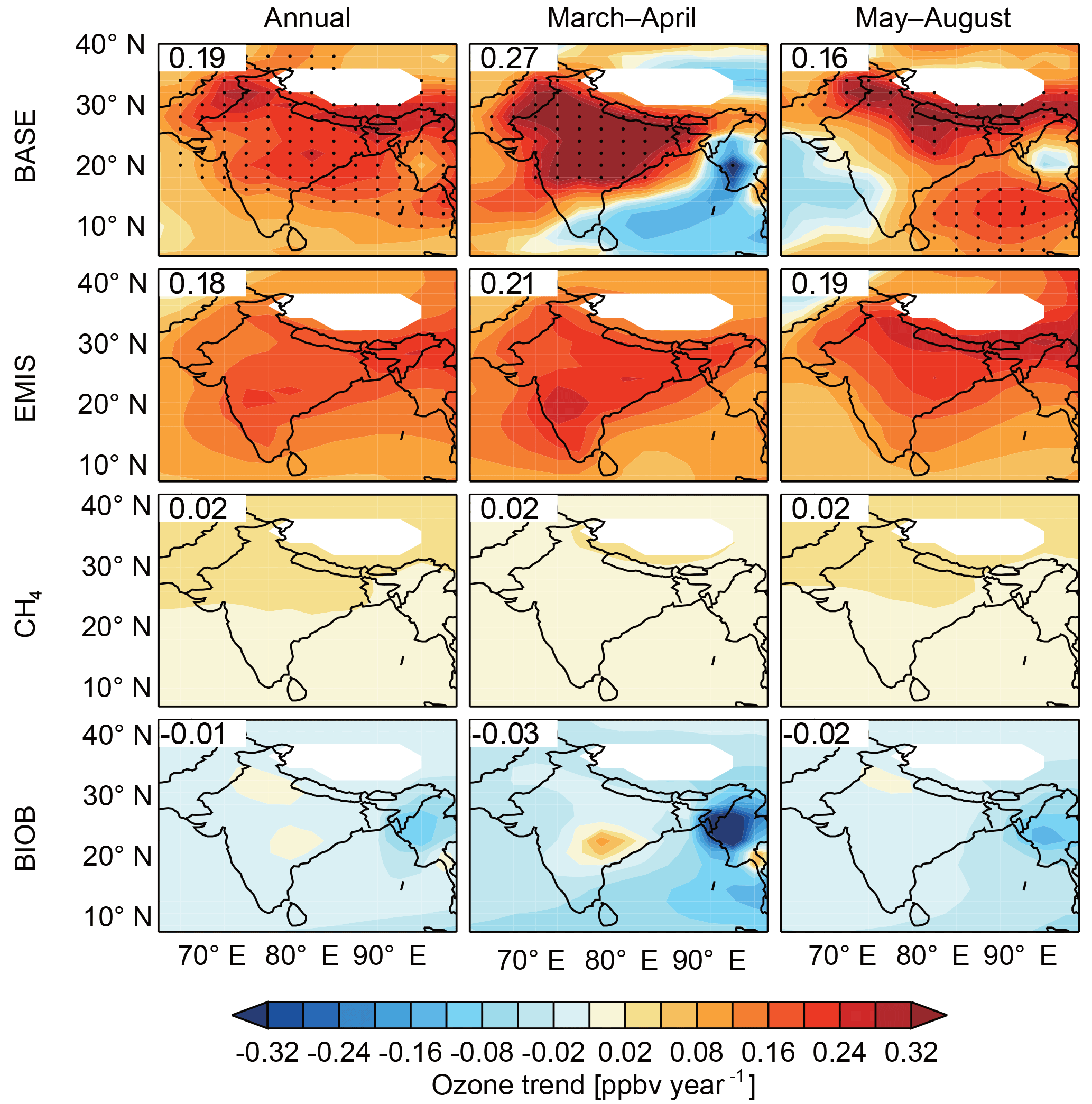
Figure 9Simulated (1990–2010) trends in lower tropospheric ozone and factors contributing to simulated trends. Trends are calculated for annual averages (left column), pre-summer monsoon seasons (central column), and summer monsoon seasons (right column). Values inset are mean trend in ppbv yr−1 averaged over the Indian land. Black dots in the first rows denote significant trends in BASE simulations. Trends contributed by interannual changes in anthropogenic emissions (EMIS), global methane concentrations (CH4), and biomass burning emissions (BIOB) are estimated.
The sensitivity simulations allow us to quantify potential ozone trend drivers, including changes in anthropogenic emissions, biomass burning emissions (Fig. S5 in the Supplement), and global methane concentrations. Figure 9 also shows the contributions from each factor calculated as differences in trends between the BASE simulation and the sensitivity simulations. Changes in anthropogenic emissions largely explain the increasing trends in lower tropospheric ozone over India, which account for 0.18, 0.21, and 0.19 ppbv yr−1 of the annual, pre-summer monsoon seasonal, and summer monsoon seasonal means, respectively. Increasing anthropogenic NO emissions (about 3 % yr−1, Fig. S5 in the Supplement) likely dominate ozone increases due to the NOx-limited ozone production condition over this region as discussed above. Global methane concentration increases also contribute to small increases of 0.02 ppbv yr−1 in the lower tropospheric ozone, and the contributions are larger in the middle and upper troposphere (figure not shown). Biomass burning emissions in East and South Asia showed a decreasing trend over 1990–2010 (Fig. S5 in the Supplement) that resulted in small negative trend contributions in the lower tropospheric ozone. As anthropogenic emissions in India are projected to rise in the future (Ghude et al., 2016), one may expect further increases in Indian tropospheric ozone. Continuous ozone monitoring measurements are required to better quantify long-term changes in tropospheric ozone over India.
In summary, we investigated the processes controlling seasonal and interannual variations in the lower tropospheric ozone concentrations over India and their linkages to the South Asian summer monsoon. We use OMI satellite observations of lower tropospheric ozone made over 2006–2014 and GEOS-Chem global model simulations over 1990–2010 driven by assimilated meteorological fields and best-known emissions to better quantify the controlling processes.
Both OMI satellite observations and GEOS-Chem simulations show that ozone in the Indian lower troposphere (surface to 600 hPa) peaks in the pre-summer monsoon season (March–April, 54.1 ppbv), and decreases dramatically to the annual minimum (40.5 ppbv) during the summer monsoon season (May–August). It then increases again in the post-summer monsoon season (September–October), and levels out in winter. GEOS-Chem process analyses on the Indian lower tropospheric ozone budget indicate that the pre-summer monsoon seasonal ozone maximum is mainly driven by enhanced ozone chemical production due to favorable meteorological conditions (strong solar radiation with low cloud cover, high temperature, and relatively dry air), as well as active biomass burning emissions in spring. We find that overall horizontal transport is important for ventilating lower tropospheric ozone, while vertical transport has a positive contribution on the lower tropospheric ozone budget over India in the pre-summer monsoon season.
The onset and evolution of the summer monsoon in May–August brings low temperatures, weak solar radiation conditions and moist air from the Arabian Sea, leading to a significant reduction in ozone production (−4.2 Tg month−1 from May to August) over India. We also highlight the contribution of upward transport on the Indian lower tropospheric ozone budget in June–August (−2.9 Tg month−1), which is comparable to the change in ozone production, and potentially transports Indian ozone to other parts of the world. In the post-summer monsoon season (September–November), lower tropospheric ozone over India increases again due to weakening ozone upward transport associated with the summer monsoon retreat. In winter, low temperature conditions limit ozone production, and strong horizontal outflows largely lower the ozone burden over India.
We show that interannual variability of lower tropospheric ozone over India in pre-summer monsoon and summer monsoon seasons are strongly linked to climate variability. Both OMI observed and model simulated lower tropospheric ozone in pre-summer monsoon seasons are significantly correlated with surface temperature (r=0.55–0.58). Higher ozone–temperature correlations (r>0.7) are found over high NOx emission regions. Lower tropospheric ozone in summer monsoon seasons is strongly influenced by the South Asian monsoon strength. Comparing the five weakest South Asian summer monsoon years with the five strongest monsoon years, we find that lower tropospheric ozone levels over India are 3.4 ppbv higher in the weakest monsoon years. This is mainly due to higher temperature, drier air, and lower cloud cover which enhances ozone production, as well as less ozone vertical export. These interannual variations indicate that lower tropospheric ozone concentrations in India are potentially affected by decadal climate variability such as the El Niño–Southern Oscillation (Kumar et al., 1999) and Atlantic Multidecadal Oscillation (Lu et al., 2006).
We also analyzed the long-term trends in lower tropospheric ozone over India and their drivers as suggested by the GEOS-Chem model. Model results over 1990–2010 show an annual mean trend of 0.19 ± 0.07 ppbv yr−1, which is mainly driven by rising anthropogenic emissions with small contributions (0.02 ppbv yr−1) from global methane concentration increases. Our study emphasizes the importance of understanding tropospheric ozone changes and drivers at multiple time scales in India. Ozone pollution in India may become more severe due to increasing anthropogenic emissions and population, and could potentially exert large impacts on the global tropospheric ozone distribution due to frequent deep convection over South Asia. Analyses of long-term ozone measurements in India are needed to better understand ozone variations and the associated environmental effects.
The datasets including measurements and model simulations used in this study can be accessed by contacting the corresponding author (Lin Zhang; zhanglg@pku.edu.cn).
The supplement related to this article is available online at: https://doi.org/10.5194/acp-18-3101-2018-supplement.
The authors declare that they have no conflict of interest.
This work is supported by the National Natural Science Foundation of China
(41475112) and China's National Basic Research Program (2014CB441303).
Xiao Lu is also supported by the Chinese Scholarship Council. The authors
thank Daniel Jacob at Harvard University for the useful comments. The authors
acknowledge the Harvard GEOS-Chem Support Team for the model maintenance and
development.
Edited by: Patrick
Jöckel
Reviewed by: two anonymous referees
Amos, H. M., Jacob, D. J., Holmes, C. D., Fisher, J. A., Wang, Q., Yantosca, R. M., Corbitt, E. S., Galarneau, E., Rutter, A. P., Gustin, M. S., Steffen, A., Schauer, J. J., Graydon, J. A., Louis, V. L. S., Talbot, R. W., Edgerton, E. S., Zhang, Y., and Sunderland, E. M.: Gas-particle partitioning of atmospheric Hg(II) and its effect on global mercury deposition, Atmos. Chem. Phys., 12, 591–603, 10.5194/acp-12-591-2012, 2012.
Beig, G. and Brasseur, G. P.: Influence of anthropogenic emissions on tropospheric ozone and its precursors over the Indian tropical region during a monsoon, Geophys. Res. Lett., 33, L07808, https://doi.org/10.1029/2005gl024949, 2006.
Beig, G., Gunthe, S., and Jadhav, D. B.: Simultaneous measurements of ozone and its precursors on a diurnal scale at a semi urban site in India, J. Atmos. Chem., 57, 239–253, https://doi.org/10.1007/s10874-007-9068-8, 2007.
Bey, I., Jacob, D. J., Yantosca, R. M., Logan, J. A., Field, B. D., Fiore, A. M., Li, Q., Liu, H. Y., Mickley, L. J., and Schultz, M. G.: Global modeling of tropospheric chemistry with assimilated meteorology: Model description and evaluation, J. Geophys. Res., 106, 23073–23095, https://doi.org/10.1029/2001jd000807, 2001.
Bhattacharjee, P. S., Singh, R. P., and Nédélec, P.: Vertical profiles of carbon monoxide and ozone from MOZAIC aircraft over Delhi, India during 2003–2005, Meteorol. Atmos. Phys., 127, 229–240, https://doi.org/10.1007/s00703-014-0349-x, 2015.
Bian, H. and Prather, M. J.: Fast-J2: Accurate Simulation of Stratospheric Photolysis in Global Chemical Models, J. Atmos. Chem., 41, 281–296, https://doi.org/10.1023/a:1014980619462, 2002.
Cooper, O. R., Gao, R.-S., Tarasick, D., Leblanc, T., and Sweeney, C.: Long-term ozone trends at rural ozone monitoring sites across the United States, 1990–2010, J. Geophys. Res., 117, D22307, https://doi.org/10.1029/2012jd018261, 2012.
Cooper, O. R., Parrish, D. D., Ziemke, J., Balashov, N. V., Cupeiro, M., Galbally, I. E., Gilge, S., Horowitz, L., Jensen, N. R., Lamarque, J. F., Naik, V., Oltmans, S. J., Schwab, J., Shindell, D. T., Thompson, A. M., Thouret, V., Wang, Y., and Zbinden, R. M.: Global distribution and trends of tropospheric ozone: An observation-based review, Elementa, 2, 000029, https://doi.org/10.12952/journal.elementa.000029, 2014.
David, L. M. and Nair, P. R.: Diurnal and seasonal variability of surface ozone and NOx at a tropical coastal site: Association with mesoscale and synoptic meteorological conditions, J. Geophys. Res., 116, D10303, https://doi.org/10.1029/2010jd015076, 2011.
Ding, A. J., Wang, T., Thouret, V., Cammas, J.-P., and Nédélec, P.: Tropospheric ozone climatology over Beijing: analysis of aircraft data from the MOZAIC program, Atmos. Chem. Phys., 8, 1–13, https://doi.org/10.5194/acp-8-1-2008, 2008.
Ding, A. J., Fu, C. B., Yang, X. Q., Sun, J. N., Zheng, L. F., Xie, Y. N., Herrmann, E., Nie, W., Petäjä, T., Kerminen, V.-M., and Kulmala, M.: Ozone and fine particle in the western Yangtze River Delta: an overview of 1 yr data at the SORPES station, Atmos. Chem. Phys., 13, 5813–5830, https://doi.org/10.5194/acp-13-5813-2013, 2013.
Ding, Y. and Chan, J. C. L.: The East Asian summer monsoon: an overview, Meteorol. Atmos. Phys., 89, 117–142, https://doi.org/10.1007/s00703-005-0125-z, 2005.
Doherty, R. M., Wild, O., Shindell, D. T., Zeng, G., MacKenzie, I. A., Collins, W. J., Fiore, A. M., Stevenson, D. S., Dentener, F. J., Schultz, M. G., Hess, P., Derwent, R. G., and Keating, T. J.: Impacts of climate change on surface ozone and intercontinental ozone pollution: A multi-model study, J. Geophys. Res., 118, 3744–3763, https://doi.org/10.1002/jgrd.50266, 2013.
Dufour, G., Eremenko, M., Orphal, J., and Flaud, J.-M.: IASI observations of seasonal and day-to-day variations of tropospheric ozone over three highly populated areas of China: Beijing, Shanghai, and Hong Kong, Atmos. Chem. Phys., 10, 3787–3801, https://doi.org/10.5194/acp-10-3787-2010, 2010.
Fiore, A. M., Oberman, J. T., Lin, M. Y., Zhang, L., Clifton, O. E., Jacob, D. J., Naik, V., Horowitz, L. W., Pinto, J. P., and Milly, G. P.: Estimating North American background ozone in U.S. surface air with two independent global models: Variability, uncertainties, and recommendations, Atmos. Environ., 96, 284–300, https://doi.org/10.1016/j.atmosenv.2014.07.045, 2014.
Gadgil, S.: The Indian monsoon and its variability, Annu. Rev. Earth Planet. Sc., 31, 429–467, https://doi.org/10.1146/annurev.earth.31.100901.141251, 2003.
Geddes, J. A., Martin, R. V., Boys, B. L., and van Donkelaar, A.: Long-Term Trends Worldwide in Ambient NO2 Concentrations Inferred from Satellite Observations, Environ. Health Persp., 124, 281–289, https://doi.org/10.1289/ehp.1409567, 2016.
Ghude, S. D., Chate, D. M., Jena, C., Beig, G., Kumar, R., Barth, M. C., Pfister, G. G., Fadnavis, S., and Pithani, P.: Premature mortality in India due to PM2.5 and ozone exposure, Geophys. Res. Lett., 43, 4650–4658, https://doi.org/10.1002/2016gl068949, 2016.
Guenther, A., Karl, T., Harley, P., Wiedinmyer, C., Palmer, P. I., and Geron, C.: Estimates of global terrestrial isoprene emissions using MEGAN (Model of Emissions of Gases and Aerosols from Nature), Atmos. Chem. Phys., 6, 3181–3210, https://doi.org/10.5194/acp-6-3181-2006, 2006.
Hou, X., Zhu, B., Fei, D., and Wang, D.: The impacts of summer monsoons on the ozone budget of the atmospheric boundary layer of the Asia-Pacific region, Sci. Total Environ., 502, 641–649, https://doi.org/10.1016/j.scitotenv.2014.09.075, 2015.
Hu, L., Jacob, D. J., Liu, X., Zhang, Y., Zhang, L., Kim, P. S., Sulprizio, M. P., and Yantosca, R. M.: Global budget of tropospheric ozone: Evaluating recent model advances with satellite (OMI), aircraft (IAGOS), and ozonesonde observations, Atmos. Environ., 167, 323–334, https://doi.org/10.1016/j.atmosenv.2017.08.036, 2017.
Huang, G., Liu, X., Chance, K., Yang, K., Bhartia, P. K., Cai, Z., Allaart, M., Ancellet, G., Calpini, B., Coetzee, G. J. R., Cuevas-Agulló, E., Cupeiro, M., De Backer, H., Dubey, M. K., Fuelberg, H. E., Fujiwara, M., Godin-Beekmann, S., Hall, T. J., Johnson, B., Joseph, E., Kivi, R., Kois, B., Komala, N., König-Langlo, G., Laneve, G., Leblanc, T., Marchand, M., Minschwaner, K. R., Morris, G., Newchurch, M. J., Ogino, S.-Y., Ohkawara, N., Piters, A. J. M., Posny, F., Querel, R., Scheele, R., Schmidlin, F. J., Schnell, R. C., Schrems, O., Selkirk, H., Shiotani, M., Skrivánková, P., Stübi, R., Taha, G., Tarasick, D. W., Thompson, A. M., Thouret, V., Tully, M. B., Van Malderen, R., Vömel, H., von der Gathen, P., Witte, J. C., and Yela, M.: Validation of 10-year SAO OMI Ozone Profile (PROFOZ) product using ozonesonde observations, Atmos. Meas. Tech., 10, 2455–2475, https://doi.org/10.5194/amt-10-2455-2017, 2017.
Huang, G., Liu, X., Chance, K., Yang, K., and Cai, Z.: Validation of 10-year SAO OMI ozone profile (PROFOZ) product using Aura MLS measurements, Atmos. Meas. Tech., 11, 17–32, https://doi.org/10.5194/amt-11-17-2018, 2018.
Hudman, R. C., Moore, N. E., Mebust, A. K., Martin, R. V., Russell, A. R., Valin, L. C., and Cohen, R. C.: Steps towards a mechanistic model of global soil nitric oxide emissions: implementation and space based-constraints, Atmos. Chem. Phys., 12, 7779–7795, https://doi.org/10.5194/acp-12-7779-2012, 2012.
IUPAC: Task group on atmospheric chemical kinetic data evaluation by International Union of Pure and Applied Chemistry (IUPAC), available at: http://iupac.pole-ether.fr/ (last access: 2 March 2018), 2013.
Jacob, D.: Heterogeneous chemistry and tropospheric ozone, Atmos. Environ., 34, 2131–2159, https://doi.org/10.1016/s1352-2310(99)00462-8, 2000.
Jacob, D. J. and Winner, D. A.: Effect of climate change on air quality, Atmos. Environ., 43, 51–63, https://doi.org/10.1016/j.atmosenv.2008.09.051, 2009.
Jaffe, D., Chand, D., Hafner, W., Westerling, A., and Spracklen, D.: Influence of fires on O3 concentrations in the Western U.S, Environ. Sci. Technol., 42, 5885–5891, https://doi.org/10.1021/es800084k, 2008.
Keller, C. A., Long, M. S., Yantosca, R. M., Da Silva, A. M., Pawson, S., and Jacob, D. J.: HEMCO v1.0: a versatile, ESMF-compliant component for calculating emissions in atmospheric models, Geosci. Model Dev., 7, 1409–1417, https://doi.org/10.5194/gmd-7-1409-2014, 2014.
Kim, P. S., Jacob, D. J., Liu, X., Warner, J. X., Yang, K., Chance, K., Thouret, V., and Nedelec, P.: Global ozone–CO correlations from OMI and AIRS: constraints on tropospheric ozone sources, Atmos. Chem. Phys., 13, 9321–9335, https://doi.org/10.5194/acp-13-9321-2013, 2013.
Krotkov, N. A., McLinden, C. A., Li, C., Lamsal, L. N., Celarier, E. A., Marchenko, S. V., Swartz, W. H., Bucsela, E. J., Joiner, J., Duncan, B. N., Boersma, K. F., Veefkind, J. P., Levelt, P. F., Fioletov, V. E., Dickerson, R. R., He, H., Lu, Z., and Streets, D. G.: Aura OMI observations of regional SO2 and NO2 pollution changes from 2005 to 2015, Atmos. Chem. Phys., 16, 4605–4629, https://doi.org/10.5194/acp-16-4605-2016, 2016.
Kuhns, H., Knipping, E. M., and Vukovich, J. M.: Development of a United States–Mexico Emissions Inventory for the Big Bend Regional Aerosol and Visibility Observational (BRAVO) Study, J. Air Waste Manage., 55, 677–692, https://doi.org/10.1080/10473289.2005.10464648, 2005.
Kumar, K. K., Rajagopalan, B., and Cane, K. A.: On the weakening relationship between the Indian Monsoon and ENSO, Science, 284, 2156–2159, https://doi.org/10.1126/science.284.5423.2156, 1999.
Kumar, R., Naja, M., Venkataramani, S., and Wild, O.: Variations in surface ozone at Nainital: A high-altitude site in the central Himalayas, J. Geophys. Res., 115, D16302, https://doi.org/10.1029/2009jd013715, 2010.
Kumar, R., Naja, M., Pfister, G. G., Barth, M. C., Wiedinmyer, C., and Brasseur, G. P.: Simulations over South Asia using the Weather Research and Forecasting model with Chemistry (WRF-Chem): chemistry evaluation and initial results, Geosci. Model Dev., 5, 619–648, https://doi.org/10.5194/gmd-5-619-2012, 2012.
Lal, S., Naja, M., and Subbaraya, B. H.: Seasonal variations in surface ozone and its precursors over an urban site in India, Atmos. Environ., 34, 2713–2724, https://doi.org/10.1016/S1352-2310(99)00510-5, 2000.
Lal, S., Venkataramani, S., Srivastava, S., Gupta, S., Mallik, C., Naja, M., Sarangi, T., Acharya, Y. B., and Liu, X.: Transport effects on the vertical distribution of tropospheric ozone over the tropical marine regions surrounding India, J. Geophys. Res., 118, 1513–1524, https://doi.org/10.1002/jgrd.50180, 2013.
Lal, S., Venkataramani, S., Chandra, N., Cooper, O. R., Brioude, J., and Naja, M.: Transport effects on the vertical distribution of tropospheric ozone over western India, J. Geophys. Res., 119, 10012–10026, https://doi.org/10.1002/2014jd021854, 2014.
Lamarque, J.-F., Bond, T. C., Eyring, V., Granier, C., Heil, A., Klimont, Z., Lee, D., Liousse, C., Mieville, A., Owen, B., Schultz, M. G., Shindell, D., Smith, S. J., Stehfest, E., Van Aardenne, J., Cooper, O. R., Kainuma, M., Mahowald, N., McConnell, J. R., Naik, V., Riahi, K., and van Vuuren, D. P.: Historical (1850–2000) gridded anthropogenic and biomass burning emissions of reactive gases and aerosols: methodology and application, Atmos. Chem. Phys., 10, 7017–7039, https://doi.org/10.5194/acp-10-7017-2010, 2010.
Lawrence, M. G. and Lelieveld, J.: Atmospheric pollutant outflow from southern Asia: a review, Atmos. Chem. Phys., 10, 11017–11096, https://doi.org/10.5194/acp-10-11017-2010, 2010.
Lelieveld, J., Crutzen, P. J., Ramanathan, V., Andreae, M. O., Brenninkmeijer, C. M., Campos, T., Cass, G. R., Dickerson, R. R., Fischer, H., de Gouw, J. A., Hansel, A., Jefferson, A., Kley, D., de Laat, A. T., Lal, S., Lawrence, M. G., Lobert, J. M., Mayol-Bracero, O. L., Mitra, A. P., Novakov, T., Oltmans, S. J., Prather, K. A., Reiner, T., Rodhe, H., Scheeren, H. A., Sikka, D., and Williams, J.: The Indian Ocean experiment: widespread air pollution from South and Southeast Asia, Science, 291, 1031–1036, https://doi.org/10.1126/science.1057103, 2001.
Levelt, P. F., van den Oord, G. H. J., Dobber, M. R., Malkki, A., Huib, V., Johan de, V., Stammes, P., Lundell, J. O. V., and Saari, H.: The ozone monitoring instrument, IEEE T. Geosci. Remote Sens., 44, 1093–1101, https://doi.org/10.1109/tgrs.2006.872333, 2006.
Li, J. and Zeng, Q.: A unified monsoon index, Geophys. Res. Lett., 29, 115-111–115-114, https://doi.org/10.1029/2001gl013874, 2002.
Li, M., Zhang, Q., Kurokawa, J.-I., Woo, J.-H., He, K., Lu, Z., Ohara, T., Song, Y., Streets, D. G., Carmichael, G. R., Cheng, Y., Hong, C., Huo, H., Jiang, X., Kang, S., Liu, F., Su, H., and Zheng, B.: MIX: a mosaic Asian anthropogenic emission inventory under the international collaboration framework of the MICS-Asia and HTAP, Atmos. Chem. Phys., 17, 935–963, https://doi.org/10.5194/acp-17-935-2017, 2017.
Lin, J.-T. and McElroy, M. B.: Impacts of boundary layer mixing on pollutant vertical profiles in the lower troposphere: Implications to satellite remote sensing, Atmos. Environ., 44, 1726–1739, 10.1016/j.atmosenv.2010.02.009, 2010.
Lin, M., Horowitz, L. W., Payton, R., Fiore, A. M., and Tonnesen, G.: US surface ozone trends and extremes from 1980 to 2014: quantifying the roles of rising Asian emissions, domestic controls, wildfires, and climate, Atmos. Chem. Phys., 17, 2943–2970, https://doi.org/10.5194/acp-17-2943-2017, 2017.
Liu, F., Beirle, S., Zhang, Q., van der A, R. J., Zheng, B., Tong, D., and He, K.: NOx emission trends over Chinese cities estimated from OMI observations during 2005 to 2015, Atmos. Chem. Phys., 17, 9261–9275, https://doi.org/10.5194/acp-17-9261-2017, 2017.
Liu, H., Jacob, D. J., Bey, I., and Yantosca, R. M.: Constraints from 210Pb and 7Be on wet deposition and transport in a global three-dimensional chemical tracer model driven by assimilated meteorological fields, J. Geophys. Res., 106, 12109-12128, 10.1029/2000jd900839, 2001.
Liu, X., Bhartia, P. K., Chance, K., Spurr, R. J. D., and Kurosu, T. P.: Ozone profile retrievals from the Ozone Monitoring Instrument, Atmos. Chem. Phys., 10, 2521–2537, https://doi.org/10.5194/acp-10-2521-2010, 2010.
Liu, Y., Wang, Y., Liu, X., Cai, Z., and Chance, K.: Tibetan middle tropospheric ozone minimum in June discovered from GOME observations, Geophys. Res. Lett., 36, L05814, https://doi.org/10.1029/2008gl037056, 2009.
Lou, S., Liao, H., Yang, Y., and Mu, Q.: Simulation of the interannual variations of tropospheric ozone over China: Roles of variations in meteorological parameters and anthropogenic emissions, Atmos. Environ., 122, 839–851, https://doi.org/10.1016/j.atmosenv.2015.08.081, 2015.
Lu, R., Dong, B., and Ding, H.: Impact of the Atlantic Multidecadal Oscillation on the Asian summer monsoon, Geophys. Res. Lett., 33, L24701, https://doi.org/10.1029/2006gl027655, 2006.
Lu, X., Zhang, L., Yue, X., Zhang, J., Jaffe, D. A., Stohl, A., Zhao, Y., and Shao, J.: Wildfire influences on the variability and trend of summer surface ozone in the mountainous western United States, Atmos. Chem. Phys., 16, 14687–14702, https://doi.org/10.5194/acp-16-14687-2016, 2016.
Mao, J., Jacob, D. J., Evans, M. J., Olson, J. R., Ren, X., Brune, W. H., Clair, J. M. St., Crounse, J. D., Spencer, K. M., Beaver, M. R., Wennberg, P. O., Cubison, M. J., Jimenez, J. L., Fried, A., Weibring, P., Walega, J. G., Hall, S. R., Weinheimer, A. J., Cohen, R. C., Chen, G., Crawford, J. H., McNaughton, C., Clarke, A. D., Jaeglé, L., Fisher, J. A., Yantosca, R. M., Le Sager, P., and Carouge, C.: Chemistry of hydrogen oxide radicals (HOx) in the Arctic troposphere in spring, Atmos. Chem. Phys., 10, 5823–5838, https://doi.org/10.5194/acp-10-5823-2010, 2010.
Mao, J., Paulot, F., Jacob, D. J., Cohen, R. C., Crounse, J. D., Wennberg, P. O., Keller, C. A., Hudman, R. C., Barkley, M. P., and Horowitz, L. W.: Ozone and organic nitrates over the eastern United States: Sensitivity to isoprene chemistry, J. Geophys. Res., 118, 11256–11268, https://doi.org/10.1002/jgrd.50817, 2013.
Mari, C., Jacob, D. J., and Bechtold, P.: Transport and scavenging of soluble gases in a deep convective cloud, J. Geophys. Res., 105, 22255–22267, 10.1029/2000jd900211, 2000.
McLinden, C. A., Olsen, S. C., Hannegan, B., Wild, O., Prather, M. J., and Sundet, J.: Stratospheric ozone in 3-D models: A simple chemistry and the cross-tropopause flux, J. Geophys. Res., 105, 14653–14665, 10.1029/2000jd900124, 2000.
McPeters, R. D., Labow, G. J., and Logan, J. A.: Ozone climatological profiles for satellite retrieval algorithms, J. Geophys. Res., 112, D05308, https://doi.org/10.1029/2005jd006823, 2007.
Monks, P. S., Archibald, A. T., Colette, A., Cooper, O., Coyle, M., Derwent, R., Fowler, D., Granier, C., Law, K. S., Mills, G. E., Stevenson, D. S., Tarasova, O., Thouret, V., von Schneidemesser, E., Sommariva, R., Wild, O., and Williams, M. L.: Tropospheric ozone and its precursors from the urban to the global scale from air quality to short-lived climate forcer, Atmos. Chem. Phys., 15, 8889–8973, https://doi.org/10.5194/acp-15-8889-2015, 2015.
Murray, L. T., Jacob, D. J., Logan, J. A., Hudman, R. C., and Koshak, W. J.: Optimized regional and interannual variability of lightning in a global chemical transport model constrained by LIS/OTD satellite data, J. Geophys. Res., 117, D20307, https://doi.org/10.1029/2012jd017934, 2012.
Murray, L. T., Logan, J. A., and Jacob, D. J.: Interannual variability in tropical tropospheric ozone and OH: The role of lightning, J. Geophys. Res., 118, 11468–11480, https://doi.org/10.1002/jgrd.50857, 2013.
Myhre, G., Shindell, D., Bréon, F.-M., Collins, W., Fuglestvedt, J., Huang, J., Koch, D., Lamarque, J.-F., Lee, D., Mendoza, B., Nakajima, T., Robock, A., Stephens, G., Takemura, T., and Zhang, H.: Anthropogenic and Natural Radiative Forcing, in: Climate Change, The Physical Science Base, Contribution of Working Group 1 to the Fifth Assessment report of the intergovernmental panel on climate change, Cambridge, UK, 2013.
Naja, M. and Lal, S.: Surface ozone and precursor gases at Gadanki (13.5∘ N, 79.2∘ E), a tropical rural site in India, J. Geophys. Res., 107, 4197, https://doi.org/10.1029/2001jd000357, 2002.
Naja, M., Lal, S., and Chand, D.: Diurnal and seasonal variabilities in surface ozone at a high altitude site Mt Abu (24.6∘ N, 72.7∘ E, 1680 m a.s.l.) in India, Atmos. Environ., 37, 4205–4215, https://doi.org/10.1016/s1352-2310(03)00565-x, 2003.
Ojha, N., Naja, M., Singh, K. P., Sarangi, T., Kumar, R., Lal, S., Lawrence, M. G., Butler, T. M., and Chandola, H. C.: Variabilities in ozone at a semi-urban site in the Indo-Gangetic Plain region: Association with the meteorology and regional processes, J. Geophys. Res., 117, D20301, https://doi.org/10.1029/2012jd017716, 2012.
Ojha, N., Naja, M., Sarangi, T., Kumar, R., Bhardwaj, P., Lal, S., Venkataramani, S., Sagar, R., Kumar, A., and Chandola, H. C.: On the processes influencing the vertical distribution of ozone over the central Himalayas: Analysis of yearlong ozonesonde observations, Atmos. Environ., 88, 201–211, https://doi.org/10.1016/j.atmosenv.2014.01.031, 2014.
Ojha, N., Pozzer, A., Rauthe-Schöch, A., Baker, A. K., Yoon, J., Brenninkmeijer, C. A. M., and Lelieveld, J.: Ozone and carbon monoxide over India during the summer monsoon: regional emissions and transport, Atmos. Chem. Phys., 16, 3013–3032, https://doi.org/10.5194/acp-16-3013-2016, 2016.
Ojha, N., Pozzer, A., Akritidis, D., and Lelieveld, J.: Secondary ozone peaks in the troposphere over the Himalayas, Atmos. Chem. Phys., 17, 6743–6757, https://doi.org/10.5194/acp-17-6743-2017, 2017.
Oltmans, S. J., Lefohn, A. S., Shadwick, D., Harris, J. M., Scheel, H. E., Galbally, I., Tarasick, D. W., Johnson, B. J., Brunke, E. G., Claude, H., Zeng, G., Nichol, S., Schmidlin, F., Davies, J., Cuevas, E., Redondas, A., Naoe, H., Nakano, T., and Kawasato, T.: Recent tropospheric ozone changes – A pattern dominated by slow or no growth, Atmos. Environ., 67, 331–351, https://doi.org/10.1016/j.atmosenv.2012.10.057, 2013.
Park, M., Randel, W. J., Gettelman, A., Massie, S. T., and Jiang, J. H.: Transport above the Asian summer monsoon anticyclone inferred from Aura Microwave Limb Sounder tracers, J. Geophys. Res., 112, D16309, https://doi.org/10.1029/2006jd008294, 2007.
Park, R. J., Jacob, D. J., Field, B. D., Yantosca, R. M., and Chin, M.: Natural and transboundary pollution influences on sulfate-nitrate-ammonium aerosols in the United States: Implications for policy, J. Geophys. Res.-Atmos., 109, D15204, https://doi.org/10.1029/2003jd004473, 2004.
Parrish, D. D., Law, K. S., Staehelin, J., Derwent, R., Cooper, O. R., Tanimoto, H., Volz-Thomas, A., Gilge, S., Scheel, H.-E., Steinbacher, M., and Chan, E.: Long-term changes in lower tropospheric baseline ozone concentrations at northern mid-latitudes, Atmos. Chem. Phys., 12, 11485–11504, https://doi.org/10.5194/acp-12-11485-2012, 2012.
Parrish, D. D., Law, K. S., Staehelin, J., Derwent, R., Cooper, O. R., Tanimoto, H., Volz-Thomas, A., Gilge, S., Scheel, H. E., Steinbacher, M., and Chan, E.: Lower tropospheric ozone at northern midlatitudes: Changing seasonal cycle, Geophys. Res. Lett., 40, 1631–1636, https://doi.org/10.1002/grl.50303, 2013.
Price, C. and Rind, D.: A simple lightning parameterization for calculating global lightning distributions, J. Geophys. Res., 97, 9919–9933, https://doi.org/10.1029/92jd00719, 1992.
Pusede, S. E., Steiner, A. L., and Cohen, R. C.: Temperature and recent trends in the chemistry of continental surface ozone, Chem. Rev., 115, 3898–3918, https://doi.org/10.1021/cr5006815, 2015.
Ramanathan, V. Sundar, S., Harnish, R., Sharma, S., Seddon, J., Croes, B., Lloyd, A., Tripathi, S. N., Aggarwal, A., Al Delaimy, W., Bahadur, R., Bandivadekar, A., Beig, G., Burney, J., Davis, S., Dutta, A., Gandhi, K. K., Guttikunda, S., Iyer, N., Joshi, T. K., Kirchstetter, T., Kubsh, J., Ramanathan, N., Rehman, I. H., Victor, D. G., Vijayan, A., Waugh, M., and Yeh, S.: India California Air Pollution Mitigation Program: Options to reduce road transport pollution in India, The Energy and Resources Institute in collaboration with the University of California at San Diego and the California Air Resources Board, 2014.
Reddy, R. R., Gopal, K. R., Reddy, L. S. S., Narasimhulu, K., Kumar, K. R., Ahammed, Y. N., and Reddy, C. V. K.: Measurements of surface ozone at semi-arid site Anantapur (14.62∘ N, 77.65∘ E, 331 m a.s.l.) in India, J. Atmos. Chem., 59, 47–59, https://doi.org/10.1007/s10874-008-9094-1, 2008.
Rienecker, M. M., Suarez, M. J., Gelaro, R., Todling, R., Bacmeister, J., Liu, E., Bosilovich, M. G., Schubert, S. D., Takacs, L., Kim, G.-K., Bloom, S., Chen, J., Collins, D., Conaty, A., da Silva, A., Gu, W., Joiner, J., Koster, R. D., Lucchesi, R., Molod, A., Owens, T., Pawson, S., Pegion, P., Redder, C. R., Reichle, R., Robertson, F. R., Ruddick, A. G., Sienkiewicz, M., and Woollen, J.: MERRA: NASA's Modern-Era Retrospective Analysis for Research and Applications, J. Climate, 24, 3624–3648, https://doi.org/10.1175/jcli-d-11-00015.1, 2011.
Rodgers, C. D.: Inverse Methods for Atmospheric Sounding: Theory and Practice, World Scientific, Singapore, 2000.
Roy, S., Beig, G., and Jacob, D.: Seasonal distribution of ozone and its precursors over the tropical Indian region using regional chemistry-transport model, J. Geophys. Res., 113, D21307, https://doi.org/10.1029/2007jd009712, 2008.
Safieddine, S., Boynard, A., Hao, N., Huang, F., Wang, L., Ji, D., Barret, B., Ghude, S. D., Coheur, P.-F., Hurtmans, D., and Clerbaux, C.: Tropospheric ozone variability during the East Asian summer monsoon as observed by satellite (IASI), aircraft (MOZAIC) and ground stations, Atmos. Chem. Phys., 16, 10489–10500, https://doi.org/10.5194/acp-16-10489-2016, 2016.
Sahu, L. K., Lal, S., and Venkataramani, S.: Distributions of O3, CO and hydrocarbons over the Bay of Bengal: A study to assess the role of transport from southern India and marine regions during September–October 2002, Atmos. Environ., 40, 4633–4645, https://doi.org/10.1016/j.atmosenv.2006.02.037, 2006.
Sahu, L. K., Sheel, V., Kajino, M., Deushi, M., Gunthe, S. S., Sinha, P. R., Sauvage, B., Thouret, V., and Smit, H. G.: Seasonal and interannual variability of tropospheric ozone over an urban site in India: A study based on MOZAIC and CCM vertical profiles over Hyderabad, J. Geophys. Res., 119, 3615–3641, https://doi.org/10.1002/2013jd021215, 2014.
Sander, S. P., Golden, D., Kurylo, M., Moortgat, G., Wine, P., Ravishankara, A., Kolb, C., Molina, M., Finlayson-Pitts, B., and Huie, R.: Chemical kinetics and photochemical data for use in atmospheric studies, JPL Publ., 06-2, 684, 2011.
Sauvage, B., Martin, R. V., van Donkelaar, A., Liu, X., Chance, K., Jaeglé, L., Palmer, P. I., Wu, S., and Fu, T.-M.: Remote sensed and in situ constraints on processes affecting tropical tropospheric ozone, Atmos. Chem. Phys., 7, 815–838, https://doi.org/10.5194/acp-7-815-2007, 2007.
Schoeberl, M. R., Douglass, A. R., Hilsenrath, E., Bhartia, P. K., Beer, R., Waters, J. W., Gunson, M. R., Froidevaux, L., Gille, J. C., Barnett, J. J., Levelt, P. F., and DeCola, P.: Overview of the EOS aura mission, IEEE T. Geosci. Remote Sens., 44, 1066–1074, https://doi.org/10.1109/tgrs.2005.861950, 2006.
Sharma, S., Chatani, S., Mahtta, R., Goel, A., and Kumar, A.: Sensitivity analysis of ground level ozone in India using WRF-CMAQ models, Atmos. Environ., 131, 29–40, https://doi.org/10.1016/j.atmosenv.2016.01.036, 2016.
Sillman, S., He, D., Cardelino, C., and Imhoff, R. E.: The Use of Photochemical Indicators to Evaluate Ozone-NOx-Hydrocarbon Sensitivity: Case Studies from Atlanta, New York, and Los Angeles, J. Air Waste Manage., 47, 1030–1040, https://doi.org/10.1080/10962247.1997.11877500, 1997.
Sinha, B., Singh Sangwan, K., Maurya, Y., Kumar, V., Sarkar, C., Chandra, B. P., and Sinha, V.: Assessment of crop yield losses in Punjab and Haryana using 2 years of continuous in situ ozone measurements, Atmos. Chem. Phys., 15, 9555–9576, https://doi.org/10.5194/acp-15-9555-2015, 2015.
Sinha, V., Kumar, V., and Sarkar, C.: Chemical composition of pre-monsoon air in the Indo-Gangetic Plain measured using a new air quality facility and PTR-MS: high surface ozone and strong influence of biomass burning, Atmos. Chem. Phys., 14, 5921–5941, https://doi.org/10.5194/acp-14-5921-2014, 2014.
Srivastava, S., Lal, S., Naja, M., Venkataramani, S., and Gupta, S.: Influence of regional pollution and long range transport over western India: Analysis of ozonesonde data, Atmos. Environ., 47, 174–182, https://doi.org/10.1016/j.atmosenv.2011.11.018, 2012a.
Srivastava, S., Lal, S., Venkataramani, S., Gupta, S., and Sheel, V.: Surface distributions of O3, CO and hydrocarbons over the Bay of Bengal and the Arabian Sea during pre-monsoon season, Atmos. Environ., 47, 459–467, https://doi.org/10.1016/j.atmosenv.2011.10.023, 2012b.
Srivastava, S., Naja, M., and Thouret, V.: Influences of regional pollution and long range transport over Hyderabad using ozone data from MOZAIC, Atmos. Environ., 117, 135–146, https://doi.org/10.1016/j.atmosenv.2015.06.037, 2015.
Stevenson, D. S., Dentener, F. J., Schultz, M. G., Ellingsen, K., van Noije, T. P. C., Wild, O., Zeng, G., Amann, M., Atherton, C. S., Bell, N., Bergmann, D. J., Bey, I., Butler, T., Cofala, J., Collins, W. J., Derwent, R. G., Doherty, R. M., Drevet, J., Eskes, H. J., Fiore, A. M., Gauss, M., Hauglustaine, D. A., Horowitz, L. W., Isaksen, I. S. A., Krol, M. C., Lamarque, J. F., Lawrence, M. G., Montanaro, V., Müller, J. F., Pitari, G., Prather, M. J., Pyle, J. A., Rast, S., Rodriguez, J. M., Sanderson, M. G., Savage, N. H., Shindell, D. T., Strahan, S. E., Sudo, K., and Szopa, S.: Multimodel ensemble simulations of present-day and near-future tropospheric ozone, J. Geophys. Res., 111, D08301, https://doi.org/10.1029/2005jd006338, 2006.
Stevenson, D. S., Young, P. J., Naik, V., Lamarque, J.-F., Shindell, D. T., Voulgarakis, A., Skeie, R. B., Dalsoren, S. B., Myhre, G., Berntsen, T. K., Folberth, G. A., Rumbold, S. T., Collins, W. J., MacKenzie, I. A., Doherty, R. M., Zeng, G., van Noije, T. P. C., Strunk, A., Bergmann, D., Cameron-Smith, P., Plummer, D. A., Strode, S. A., Horowitz, L., Lee, Y. H., Szopa, S., Sudo, K., Nagashima, T., Josse, B., Cionni, I., Righi, M., Eyring, V., Conley, A., Bowman, K. W., Wild, O., and Archibald, A.: Tropospheric ozone changes, radiative forcing and attribution to emissions in the Atmospheric Chemistry and Climate Model Intercomparison Project (ACCMIP), Atmos. Chem. Phys., 13, 3063–3085, https://doi.org/10.5194/acp-13-3063-2013, 2013.
Stohl, A., Bonasoni, P., Cristofanelli, P., Collins, W., Feichter, J., Frank, A., Forster, C., Gerasopoulos, E., Gaggeler, H., James, P., Kentarchos, T., Kromp-Kolb, H., Kruger, B., Land, C., Meloen, J., Papayannis, A., Priller, A., Seibert, P., Sprenger, M., Roelofs, G. J., Scheel, H. E., Schnabel, C., Siegmund, P., Tobler, L., Trickl, T., Wernli, H., Wirth, V., Zanis, P., and Zerefos, C.: Stratosphere-troposphere exchange: A review, and what we have learned from STACCATO, J. Geophys. Res.-Atmos., 108, 8516, https://doi.org/10.1029/2002jd002490, 2003.
Strode, S. A., Rodriguez, J. M., Logan, J. A., Cooper, O. R., Witte, J. C., Lamsal, L. N., Damon, M., Van Aartsen, B., Steenrod, S. D., and Strahan, S. E.: Trends and variability in surface ozone over the United States, J. Geophys. Res.-Atmos., 120, 9020–9042, https://doi.org/10.1002/2014jd022784, 2015.
Sun, L., Xue, L., Wang, T., Gao, J., Ding, A., Cooper, O. R., Lin, M., Xu, P., Wang, Z., Wang, X., Wen, L., Zhu, Y., Chen, T., Yang, L., Wang, Y., Chen, J., and Wang, W.: Significant increase of summertime ozone at Mount Tai in Central Eastern China, Atmos. Chem. Phys., 16, 10637–10650, https://doi.org/10.5194/acp-16-10637-2016, 2016.
van der Werf, G. R., Randerson, J. T., Giglio, L., Collatz, G. J., Mu, M., Kasibhatla, P. S., Morton, D. C., DeFries, R. S., Jin, Y., and van Leeuwen, T. T.: Global fire emissions and the contribution of deforestation, savanna, forest, agricultural, and peat fires (1997–2009), Atmos. Chem. Phys., 10, 11707–11735, https://doi.org/10.5194/acp-10-11707-2010, 2010.
Venkataraman, C., Habib, G., Kadamba, D., Shrivastava, M., Leon, J. F., Crouzille, B., Boucher, O., and Streets, D. G.: Emissions from open biomass burning in India: Integrating the inventory approach with high-resolution Moderate Resolution Imaging Spectroradiometer (MODIS) active-fire and land cover data, Global Biogeochem. Cy., 20, GB2013, https://doi.org/10.1029/2005gb002547, 2006.
Wang, B. and LinHo: Rainy Season of the Asian-Pacific Summer Monsoon, J. Climate, 15, 386–398, 2002.
Wang, T., Wei, X. L., Ding, A. J., Poon, C. N., Lam, K. S., Li, Y. S., Chan, L. Y., and Anson, M.: Increasing surface ozone concentrations in the background atmosphere of Southern China, 1994–2007, Atmos. Chem. Phys., 9, 6217–6227, https://doi.org/10.5194/acp-9-6217-2009, 2009.
Wang, T., Xue, L., Brimblecombe, P., Lam, Y. F., Li, L., and Zhang, L.: Ozone pollution in China: A review of concentrations, meteorological influences, chemical precursors, and effects, Sci. Total Environ., 575, 1582–1596, https://doi.org/10.1016/j.scitotenv.2016.10.081, 2017.
Wang, Y., Shen, L., Wu, S., Mickley, L., He, J., and Hao, J.: Sensitivity of surface ozone over China to 2000–2050 global changes of climate and emissions, Atmos. Environ., 75, 374–382, https://doi.org/10.1016/j.atmosenv.2013.04.045, 2013.
Wesely, M. L.: Parameterization of Surface Resistances to Gaseous Dry Deposition in Regional-Scale Numerical-Models, Atmos. Environ., 23, 1293–1304, https://doi.org/10.1016/0004-6981(89)90153-4, 1989.
Westerling, A. L., Hidalgo, H. G., Cayan, D. R., and Swetnam, T. W.: Warming and earlier spring increase western U.S. forest wildfire activity, Science, 313, 940–943, https://doi.org/10.1126/science.1128834, 2006.
Xu, X., Lin, W., Wang, T., Yan, P., Tang, J., Meng, Z., and Wang, Y.: Long-term trend of surface ozone at a regional background station in eastern China 1991–2006: enhanced variability, Atmos. Chem. Phys., 8, 2595-2607, 10.5194/acp-8-2595-2008, 2008.
Yan, Y., Lin, J., Chen, J., and Hu, L.: Improved simulation of tropospheric ozone by a global-multi-regional two-way coupling model system, Atmos. Chem. Phys., 16, 2381–2400, https://doi.org/10.5194/acp-16-2381-2016, 2016.
Yang, Y., Liao, H., and Li, J.: Impacts of the East Asian summer monsoon on interannual variations of summertime surface-layer ozone concentrations over China, Atmos. Chem. Phys., 14, 6867–6879, https://doi.org/10.5194/acp-14-6867-2014, 2014.
Young, P. J., Archibald, A. T., Bowman, K. W., Lamarque, J.-F., Naik, V., Stevenson, D. S., Tilmes, S., Voulgarakis, A., Wild, O., Bergmann, D., Cameron-Smith, P., Cionni, I., Collins, W. J., Dalsøren, S. B., Doherty, R. M., Eyring, V., Faluvegi, G., Horowitz, L. W., Josse, B., Lee, Y. H., MacKenzie, I. A., Nagashima, T., Plummer, D. A., Righi, M., Rumbold, S. T., Skeie, R. B., Shindell, D. T., Strode, S. A., Sudo, K., Szopa, S., and Zeng, G.: Pre-industrial to end 21st century projections of tropospheric ozone from the Atmospheric Chemistry and Climate Model Intercomparison Project (ACCMIP), Atmos. Chem. Phys., 13, 2063–2090, https://doi.org/10.5194/acp-13-2063-2013, 2013.
Zhang, L., Jacob, D. J., Liu, X., Logan, J. A., Chance, K., Eldering, A., and Bojkov, B. R.: Intercomparison methods for satellite measurements of atmospheric composition: application to tropospheric ozone from TES and OMI, Atmos. Chem. Phys., 10, 4725–4739, https://doi.org/10.5194/acp-10-4725-2010, 2010.
Zhang, L., Jacob, D. J., Yue, X., Downey, N. V., Wood, D. A., and Blewitt, D.: Sources contributing to background surface ozone in the US Intermountain West, Atmos. Chem. Phys., 14, 5295–5309, https://doi.org/10.5194/acp-14-5295-2014, 2014.
Zhang, L. M., Gong, S. L., Padro, J., and Barrie, L.: A size-segregated particle dry deposition scheme for an atmospheric aerosol module, Atmos. Environ., 35, 549–560, https://doi.org/10.1016/S1352-2310(00)00326-5, 2001.
Zhang, Y., Cooper, O. R., Gaudel, A., Thompson, A. M., Nédélec, P., Ogino, S.-Y., and West, J. J.: Tropospheric ozone change from 1980 to 2010 dominated by equatorward redistribution of emissions, Nat. Geosci., 9, 875–879, https://doi.org/10.1038/ngeo2827, 2016.
Zhao, Y., Zhang, L., Tai, A. P. K., Chen, Y., and Pan, Y.: Responses of surface ozone air quality to anthropogenic nitrogen deposition in the Northern Hemisphere, Atmos. Chem. Phys., 17, 9781–9796, https://doi.org/10.5194/acp-17-9781-2017, 2017.
Zhou, D., Ding, A., Mao, H., Fu, C., Wang, T., Chan, L. Y., Ding, K., Zhang, Y., Liu, J., Lu, A., and Hao, N.: Impacts of the East Asian monsoon on lower tropospheric ozone over coastal South China, Environ. Res. Lett., 8, 044011, https://doi.org/10.1088/1748-9326/8/4/044011, 2013.
Zhu, J., Liao, H., and Li, J.: Increases in aerosol concentrations over eastern China due to the decadal-scale weakening of the East Asian summer monsoon, Geophys. Res. Lett., 39, L09809, https://doi.org/10.1029/2012gl051428, 2012.
- Abstract
- Introduction
- Observations and model description
- Seasonal variation of lower tropospheric ozone over India
- Interannual variability of lower tropospheric ozone over India
- Long-term trend and contributing drivers
- Conclusions
- Data availability
- Competing interests
- Acknowledgements
- References
- Supplement