the Creative Commons Attribution 4.0 License.
the Creative Commons Attribution 4.0 License.
 | 11 Sep 2018
The importance of comprehensive parameter sampling and multiple observations for robust constraint of aerosol radiative forcing
Leighton A. Regayre
Masaru Yoshioka
Kirsty J. Pringle
Lindsay A. Lee
David M. H. Sexton
John W. Rostron
Ben B. B. Booth
Kenneth S. Carslaw
Observational constraint of simulated aerosol and cloud properties is an essential part of building trustworthy climate models for calculating aerosol radiative forcing. Models are usually tuned to achieve good agreement with observations, but tuning produces just one of many potential variants of a model, so the model uncertainty cannot be determined. Here we estimate the uncertainty in aerosol effective radiative forcing (ERF) in a tuned climate model by constraining 4 million variants of the HadGEM3-UKCA aerosol–climate model to match nine common observations (top-of-atmosphere shortwave flux, aerosol optical depth, PM2.5, cloud condensation nuclei at 0.2 % supersaturation (CCN0.2), and concentrations of sulfate, black carbon and organic carbon, as well as decadal trends in aerosol optical depth and surface shortwave radiation.) The model uncertainty is calculated by using a perturbed parameter ensemble that samples 27 uncertainties in both the aerosol model and the physical climate model, and we use synthetic observations generated from the model itself to determine the potential of each observational type to constrain this uncertainty. Focusing over Europe in July, we show that the aerosol ERF uncertainty can be reduced by about 30 % by constraining it to the nine observations, demonstrating that producing climate models with an observationally plausible “base state” can contribute to narrowing the uncertainty in aerosol ERF. However, the uncertainty in the aerosol ERF after observational constraint is large compared to the typical spread of a multi-model ensemble. Our results therefore raise questions about whether the underlying multi-model uncertainty would be larger if similar approaches as adopted here were applied more widely. The approach presented in this study could be used to identify the most effective observations for model constraint. It is hoped that aerosol ERF uncertainty can be further reduced by introducing process-related constraints; however, any such results will be robust only if the enormous number of potential model variants is explored.
- Article
(6433 KB) - Full-text XML
- BibTeX
- EndNote


It has proven extremely challenging to reduce the large uncertainty in aerosol model simulations and the calculated aerosol radiative forcing since pre-industrial times. Although extensive improvements in the physical realism of aerosol–climate models have been made in recent years (Ghan and Schwartz, 2007), resulting in a set of quite sophisticated models (Mann et al., 2014), aerosol model simulations are still surprisingly uncertain – up to a factor of 10 or more spread in key aerosol properties among models (Mann et al., 2014). Calculated aerosol radiative forcing also remains stubbornly uncertain among multiple models (Boucher et al., 2013; Myhre et al., 2013), making it difficult to establish the causes of forcing uncertainty. Until the uncertainty is reduced, climate models will not be robust in their predictions of decadal-scale climate change and its global and regional impacts (Andreae et al., 2005; Myhre et al., 2013; Seinfeld et al., 2016).
The uncertainty in aerosol radiative forcing has persisted through multiple generations of climate models because it results from the combined effects of dozens of complex and uncertain climate model processes related to aerosols, clouds, radiation and dynamics. Changes in aerosols cause the entire aerosol–cloud–radiation dynamics system to respond, resulting in an effective radiative forcing, or ERF (Boucher et al., 2013). The complexity of the processes causing the aerosol ERF (and the fact that it cannot be measured directly) means that it may essentially be treated as a tuneable model quantity (Hourdin et al., 2016; Mauritsen et al., 2012) rather than being properly constrained by extensive measurements that define the state and behaviour of aerosols and clouds. This is not a firm basis for climate projections.
There are three ways in which observations help to constrain the uncertainty in aerosol ERF. The first, which applies to the aerosol–cloud-related forcing, is based on the recognition that the forcing depends on the interlinked sensitivities of aerosols, clouds and their radiative properties to changes in aerosol emissions. For example, the magnitude of the aerosol–cloud interaction component of radiative forcing (R) can be broken down into a product of sensitivities relating the forcing to aerosol emissions (E), cloud condensation nuclei concentrations (NCCN) and droplet concentrations (Nd) (Ghan et al., 2016):
Relationships between various aerosol, cloud and radiation variables are widely used or proposed as a way of constraining the uncertainty in aerosol–cloud forcing in climate models (Ban-weiss et al., 2014; Grandey et al., 2013; Gryspeerdt et al., 2016, 2017; Gryspeerdt and Stier, 2012; Lebo and Feingold, 2014; McCoy et al., 2016; Quaas et al., 2009, 2010; Terai et al., 2015; Yi et al., 2012; Zhang et al., 2016).
The second aspect of model constraint is to test the model's ability to reproduce observed trends in aerosols, clouds and radiation (Allen et al., 2013; Cherian et al., 2014; Leibensperger et al., 2012; Li et al., 2013; Liepert and Tegen, 2002; Shindell et al., 2013; Turnock et al., 2015; Zhang et al., 2017). For example, Cherian et al. (2014) showed that among several climate models there is a relationship between the simulated trend in European surface solar radiation (SSR) over recent decades and the pre-industrial to present-day aerosol ERF (models with large SSR trends tend to simulate larger ERFs). Cherian et al. (2014) used this relationship to define the observationally constrained ERF based on the models that simulate SSR trends closest to observations (a so-called emergent constraint).
The third aspect of model constraint is to observationally constrain the model “base state” – i.e. properties like aerosol optical depth (AOD) or aerosol concentrations in a particular period. Considerable effort is put into constraining the model base state because observations are readily available and models that cannot simulate aerosol and cloud properties close to observations would not be trusted to predict changes in these properties over time (which determines the forcing). Models can also be constrained under a range of cloud regimes as well as under pristine and polluted conditions, which will have a bearing on a model's ability to simulate the change from the pre-industrial period to the present-day (Carslaw et al., 2013, 2017). Model skill in simulating AOD was used in the Atmospheric Chemistry-Climate Model Intercomparison Project to screen the models (Shindell et al., 2013) and global AOD reanalysis products have been used to help constrain the aerosol forcing (Bellouin et al., 2013). It is also argued that the wealth of available measurements will help to constrain direct radiative forcing (Kahn, 2012).
There are limitations with all three methods outlined above in terms of constraining the uncertainty in aerosol forcing over periods outside the observational record. The main limitation with the first method (aerosol–cloud–radiation relations) is that there is no guarantee that present-day (or “instantaneous”) relationships can be extrapolated to pristine pre-industrial conditions (Penner et al., 2011). Even the most sophisticated approaches still rely on model estimates of how aerosols changed over the industrial period (Gryspeerdt et al., 2017). The same main limitation applies to the second method (aerosol and radiation trends): most data records are quite short so typically do not include pristine pre-industrial-like conditions (Carslaw et al., 2017; Hamilton et al., 2014). With the third method (constraining the state of aerosols, clouds and their radiative properties) it is not obvious how the model accuracy can be related to the uncertainty in simulated radiative forcing (i.e. there is no equivalent to Eq. 1 defining how a bias in simulated aerosol properties affects the forcing). One aim of our study is to make that link, and we show in Sect. 3.5.1 that observational constraint of many state variables only weakly constrains the direct and indirect radiative forcings.
In this paper we focus on observationally constraining uncertainty in the base state of an aerosol–climate model as well as trends in radiative properties. Our approach is shown schematically in Fig. 1. We begin with a large set of model variants produced by adjusting multiple uncertain model input parameters (a tiny fraction of which would be explored in model tuning). These model variants (parameter combinations) define the prior model uncertainty (which can be defined by a probability density function, PDF), which we then constrain by identifying variants that produce plausible outputs compared to aerosol and cloud observations. Model variants that produce implausible results (i.e. output outside of an observation's estimated uncertainty range) are rejected and, likewise, the forcings that they calculate are also rejected. A similar constraint methodology has been applied to environmental models (Salter and Williamson, 2016), hydrological models (Liu and Gupta, 2007), galaxy formation (Rodrigues et al., 2017), disease transmission (Andrianakis et al., 2017), climate models (Murphy et al., 2004; Regayre et al., 2018; Sexton et al., 2011; Williamson et al., 2013) and aerosol models (Lee et al., 2011, 2013; Reddington et al., 2017; Regayre et al., 2018, 2014, 2015). In this paper the observations comprise aerosol and cloud state variables and trends, but the approach could readily be extended to include any observations, such as of aerosol–cloud–radiation relationships. We constrain using each aerosol–cloud observation individually and the combination of all observations.
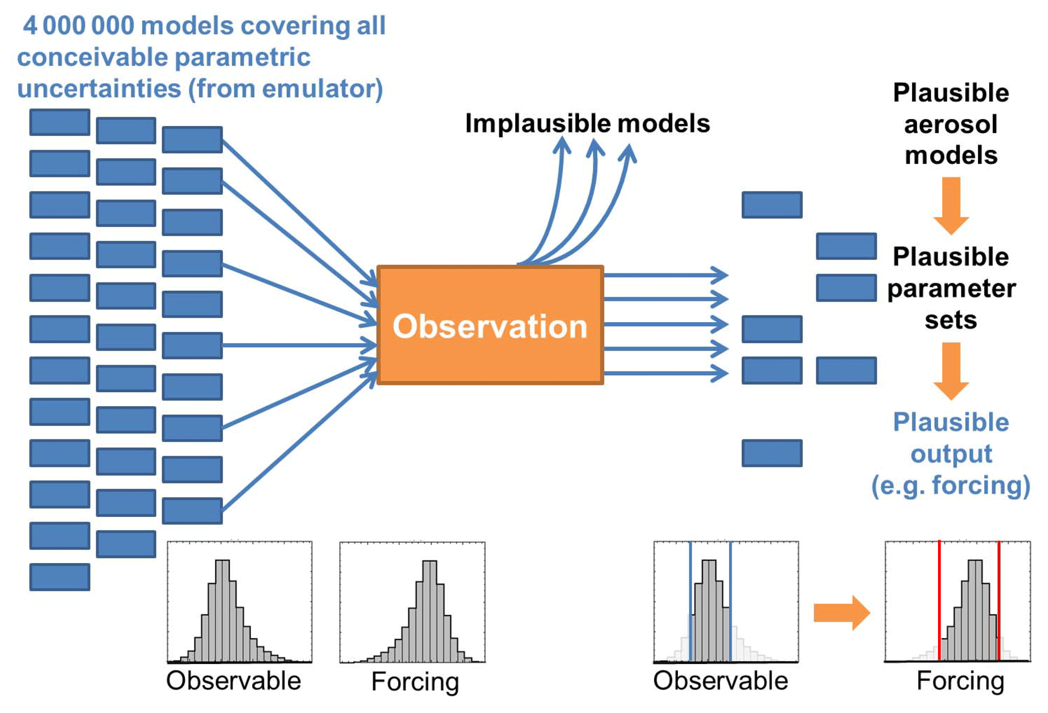
Figure 1Schematic of the methodology for observational constraint of parametric model uncertainty.
We define observational constraint as finding the full set of model variants that can be considered plausible against observations, and from which we can estimate the prior (unconstrained) and remaining (observationally constrained) uncertainty. This approach is different to traditional model tuning, which produces only one result on the right side of Fig. 1 with no information about uncertainty. We note, however, that such model adjustments towards observations are often misleadingly called constraint.
The vast majority of observational constraint efforts are severely limited by the very small number of models used, which makes it impossible to reach robust statistical conclusions about model uncertainty. In a multi-model ensemble the number of models is often about 10 or so, and in model tuning perhaps only a few dozen parts of parameter space are explored. To get around this problem we build emulators that enable model outputs to be generated for millions of model parameter combinations (Lee et al., 2011, 2013), which enables us to relate the uncertainty on the left side of Fig. 1 (in the form of a PDF) to the observationally constrained uncertainty on the right side.
The main aims of this paper are first to determine how much uncertainty could potentially remain in an aerosol–chemistry–climate model that is tuned to match various sets of observations, and second, how this uncertainty might affect conclusions drawn from multi-model ensemble studies which do not explicitly account for this source of uncertainty. Although large observational datasets of aerosol in situ microphysical and chemical properties are available (Reddington et al., 2017), we use synthetic observations here – i.e. observations that are generated from a model simulation – to postpone addressing some of the challenges faced when comparing model output and in situ observations (Schutgens et al., 2016a, b).
The analysis is restricted to the region of Europe (defined in this study by the longitude range 12∘ W to 41∘ E and latitude range 37.5 to 71.5∘ N) for the month of July. We take a regional approach primarily because regional observations provide a better constraint on model uncertainty than global mean observations (Regayre et al., 2018). The sources of uncertainty in aerosols and forcing vary regionally (Lee et al., 2016; Reddington et al., 2017; Regayre et al., 2015). Therefore, a global analysis would essentially be a scaled-up version of what we present here – i.e. a set of regional evaluations. We choose Europe in July as this is a region and month for which a distinct set of parameter uncertainties affect the aerosol properties and the ERF, providing a good test case for our methodology. Europe is also a region for which a diverse set of long-term measurements of different aerosol and radiative properties are available, that we can use to inform our assessments of observational uncertainty.
The following section describes the aerosol–climate model, the set-up of the simulations and the statistical methodology we use to sample the model uncertainty. Section 3 describes our results, starting with an analysis of the magnitude and causes of model uncertainty. We then examine the effects of observational constraint on the simulated aerosol properties, the multi-century (1850–2008) and multi-decade (1978–2008) aerosol ERF uncertainty and the plausible parameter ranges. In Sect. 4 we estimate the potential implications of our results for multi-model emergent constraint studies and other studies that use observations to screen out models.
2.1 Summary of the constraint methodology
The steps involved are as follows (Fig. 1):
-
A perturbed parameter ensemble (PPE) of the HadGEM3-UKCA aerosol–chemistry–climate model (Sect. 2.2) is created to efficiently sample combinations of 27 uncertainties related to the aerosol model and physical processes in the host climate model (mostly related to clouds). The PPE (Sect. 2.3) consists of three sets of 191 single-year simulations which differ only in the anthropogenic aerosol emissions prescribed (1850, 1978 and 2008). The use of HadGEM enables us to diagnose the aerosol ERF rather than just the cloud albedo forcing as in our previous studies (Carslaw et al., 2013; Regayre et al., 2014, 2015).
-
Emulators are built based on the PPE training data (step 1), which define (within quantifiable uncertainty) how aerosol properties and aerosol radiative forcing vary over the 27-dimensional parameter space (Sect. 2.4). We validate each emulator's ability to reproduce model output, then use them to sample the 4 million Monte Carlo points from the parameter space to produce the set of model variants on the left side of Fig. 1. This step is essential because, with 27 dimensions of model uncertainty, the 191 PPE simulations are sparsely distributed. A denser sample of the multi-dimensional parameter space from the emulator enables us to conduct robust statistical analyses.
-
The causes of uncertainty in the aerosol and forcing variables are determined using variance-based sensitivity analysis (Sect. 2.5). This step is not essential for constraining the model, but is useful for understanding which processes in the model account for the uncertainties in the outputs (Carslaw et al., 2013; Lee et al., 2013; Regayre et al., 2018, 2014, 2015).
-
A set of “synthetic” observations (Sect. 2.6) is created with realistic uncertainty ranges. We use one PPE member to define these synthetic observations.
-
We identify which of the 4 million model variants are consistent with the observations within their individual uncertainty ranges (Sect. 2.7). This reduced set of variants defines the ways in which parameter values can be combined to reproduce multiple observations and is equivalent to identifying several thousand equally plausible tuned HadGEM3-UKCA models. This procedure is often called “history matching” or “pre-calibration” (Craig et al., 1997; Edwards et al., 2011; Williamson et al., 2013; Lee et al., 2016; Andrianakis et al., 2017).
-
The reduction in aerosol ERF uncertainty is quantified using the observationally constrained parameter space (Sect. 2.8).
The observational constraint approach we apply here is quite different to aerosol data assimilation (Bellouin et al., 2013), which cannot directly estimate aerosol ERFs or the uncertainty. In principle, both approaches should generate similar distributions of AOD (the usual assimilated observation variable) if similar observations are used. However, we can directly determine aerosol ERF and its uncertainty by running the plausible model variants in both the present day (where the model uncertainty was constrained) and the pre-industrial period. In contrast, estimation of the ERF using the assimilation approach relies on assumptions about how present-day natural AOD represents pre-industrial aerosols because the approach generates only a present-day aerosol state and not a model that can be used to simulate pre-industrial conditions.
2.2 The HadGEM3-UKCA climate model
We use the UK Hadley Centre Unified Model HadGEM3 (HadGEM3, 2017), incorporating version 8.4 of the UK Chemistry and Aerosol (UKCA) model. UKCA simulates trace gas chemistry and the evolution of the aerosol particle size distribution and chemical composition using the GLObal Model of Aerosol Processes (GLOMAP-mode; Mann et al., 2010) and a whole-atmosphere chemistry scheme (O'Connor et al., 2014). The model has a horizontal resolution of 1.25×1.875∘ and 85 vertical hybrid pressure levels.
The aerosol size distribution is defined by seven log-normal modes: one soluble nucleation mode as well as soluble and insoluble Aitken, accumulation and coarse modes. The aerosol chemical components are sulfate, sea salt, black carbon (BC), organic carbon (OC) and dust. Secondary organic aerosol (SOA) material is produced from the first-stage oxidation products of biogenic monoterpenes under the assumption of zero vapour pressure. SOA is combined with primary particulate organic matter after kinetic condensation.
GLOMAP simulates new particle formation, coagulation, gas-to-particle transfer, cloud processing, and deposition of gases and aerosols. The activation of aerosols into cloud droplets is calculated using globally prescribed distributions of sub-grid vertical velocities (West et al., 2014), and the removal of cloud droplets by autoconversion to rain is calculated by the host model. Aerosols are also removed by impaction scavenging of falling raindrops according to the parametrization of clouds and precipitation collocation (Boutle et al., 2014; Lebsock et al., 2013). Aerosol water uptake efficiency is determined by kappa-Kohler theory (Petters and Kreidenweis, 2007) using composition-dependent hygroscopicity factors.
Anthropogenic emission scenarios prepared for the Atmospheric Chemistry and Climate Model Inter-comparison Project (ACCMIP) and prescribed in some of the CMIP Phase 5 experiments are used here. Carbonaceous biomass burning aerosol emissions for recent decades were prescribed using a 10-year average of 2002 to 2011 monthly mean data from the Global Fire and Emissions Database (GFED3; van der Werf et al., 2010) and according to Lamarque et al. (2010) for 1850. The prescribed volcanic SO2 emissions combine emissions from the Andres and Kasgnoc (1998) dataset for continuously erupting and sporadically erupting volcanoes and the Halmer et al. (2002) dataset for explosive volcanoes.
Horizontal winds in the simulations are nudged towards European Centre for Medium-Range Weather Forecasts (ECMWF) ERA-Interim reanalyses for 2006 between approximately 2.15 and 80 km using a 6 h relaxation timescale. Nudging means that pairs of simulations have near-identical synoptic-scale features, which enables the effects of perturbations to aerosol and chemical processes within the boundary layer to be quantified using single-year simulations. Without nudging, the model fields would need to be averaged over several decades in order to produce signals stronger than the noise caused by internal variability (Kooperman et al., 2012). By nudging horizontal winds but not temperature, liquid water path and atmospheric humidity can respond to aerosol-induced changes in temperature, allowing more of the rapid responses of clouds and radiation to aerosol perturbations to be captured.
Each simulation was subject to a 4-month spin-up period with parameters set to their median values. Parameter perturbations were then applied distinctly to individual ensemble members and spun up for a further 3 months. We analyse the data from July for each simulation following the spin-up period. The calculation of the aerosol ERF and its components is described in Sect. 2.8.
2.3 Perturbed parameter ensemble
A perturbed parameter ensemble (PPE) is a set of simulations with excellent space-filling properties that provides information about model output across the multi-dimensional space of uncertain model input parameters. The PPE, described in detail in Yoshioka et al. (2018), was specifically designed to sample aerosol as well as host physical climate model parameters of importance to the aerosol ERF. Regayre et al. (2018) show that host model parameters cause most of the uncertainty in the radiative state of the atmosphere but aerosol parameters contribute more to the uncertainty in the change of state (aerosol ERF).
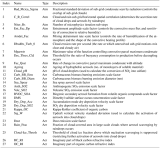
The 27 perturbed parameters are listed in Table 1. They are categorized as either aerosol (aer) or atmospheric (atm) according to their role in the model. To define the set of parameters we used expert elicitation and carried out one-at-a-time parameter perturbation screening experiments to quantify the effect of individual parameter perturbations away from the default setting. The selected parameters are described in more detail in related papers (Regayre et al., 2018; Yoshioka et al., 2018).
A total of 18 parameters related to aerosol and precursor gas emissions, deposition, and aerosol processes were perturbed based on their importance (Lee et al., 2013; Carslaw et al., 2013; Regayre et al., 2014, 2015). Several parameters available in the HadGEM3-UKCA model but not in the chemistry transport model were included after analysing the one-at-a-time perturbation screening experiments. These are the updraft velocity in shallow clouds, the fraction of large-scale cloud in which rain-scavenging of aerosols can occur, and the refractive indices of BC and OC. In some cases we perturbed similar parameters as in Regayre et al. (2014) but these parameters are handled differently within the HadGEM model. These are the dry deposition velocity of SO2, dust emissions and the fraction of ice in mixed-phase clouds above which aerosol scavenging is suppressed.
Nine physical model parameters were perturbed. These were selected from a much larger set tested by the UK Met Office in developing their ensemble prediction system (Sexton et al., 2017) based on their potential to contribute to uncertainty in a broad range of aerosol, cloud and radiation properties; in particular particle number concentrations, cloud condensation nuclei, PM2.5, aerosol optical depth, sulfate and SOA concentrations, cloud reflectivity, liquid water path, precipitation, and aerosol ERF. These nine atmospheric model parameters are considered the most likely causes of uncertainty in low-altitude clouds and aerosol–cloud interactions because they influence boundary layer clouds by altering cloud radiative properties, cloud drop concentrations and microphysical processes, atmospheric humidity, convection processes, and boundary layer stability.
A probability density function was defined for each parameter to represent shared expert beliefs about parameter uncertainty. These distributions have no effect on the model simulations (although the ranges define the span of the parameter space), but are used at the stage of generating PDFs of model output based on Monte Carlo sampling from the emulators. We used mainly trapezoidal distributions that avoid overly centralized Monte Carlo sampling of the multi-dimensional parameter space (Yoshioka et al., 2018).
Maximin Latin hypercube sampling was used to create an initial set of 162 simulations that sample model output across the 27-dimensional parameter space. A further set of 54 simulations was used to validate the emulators. In total 217 perturbed parameter simulations of the global model were run for a full year for each anthropogenic emission period (1850, 1978 and 2008 emissions). Each simulation had a spin-up period of 7 months from a consistent starting simulation, where the parameters were set to their median values for the first 4 months and the perturbations then applied in the final 3 months. A total of 25 simulations did not complete the full annual cycle and so were not used in our analysis. Consequently, the ensemble of simulations used for analysis for each period was made up of the remaining 191 simulations, all of which were used to build the final emulators. Radiative forcings were calculated as the difference in top-of-atmosphere (ToA) radiative flux for pairs of simulations with identical parameter settings but different anthropogenic emissions (1850, 1978 and 2008).
Table 1The 27 host model and aerosol parameters included in the PPE. Further details are provided in a separate publication (Regayre et al., 2018).
2.4 Model emulation and Monte Carlo sampling
For each model output (such as the regional mean ToA flux, CCN0.2 concentration, etc. for Europe in July) we construct a statistical emulator model over the 27-dimensional parameter uncertainty using the 137 training simulations and validate it using the 54 validation simulations (as described in Lee et al., 2011). Once validated, a further new emulator is then created using both the training and the validation simulations of the PPE, to obtain a final emulator based on all of the information that our simulations contain. A “leave-one-out” validation procedure (where each simulation in turn is removed from the merged set, and a new emulator is constructed and used to predict that removed simulation) is applied to additionally verify the quality of our final emulator. We then use this emulator to predict the model output for a large sample (here 4 million) of parameter input combinations that span the 27-dimensional parameter space of the PPE. From this sample we obtain a PDF of the uncertainty in this output variable caused by the defined uncertainty in the model parameters (left-hand side of Fig. 1). In each case, the output PDF can be sampled according to the elicited parameter probability distributions (Yoshioka et al., 2018), in which case the PDF accounts for prior beliefs about the likelihood of different parameter values. Alternatively uniform sampling can be applied, in which case the output PDF assumes that all parameters have equal likelihood of lying between their elicited upper and lower limits. Our approach is to use the prior probability distributions, informed by expert knowledge, to sample the parameter combinations of the 4 million model variants over the 27-dimensional parameter uncertainty space.
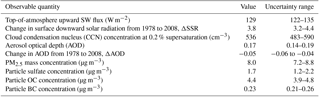
Table 2Observed quantities and corresponding uncertainty ranges used for the constraints applied over Europe. Values are a European July mean, synthetically generated from the model output of a selected PPE member.
2.5 Sensitivity analysis
Sensitivity analysis (Lee et al., 2011; Saltelli et al., 1999) is used to decompose the uncertainty in European regional mean aerosol properties, trends and forcing variables for July into contributions from each individual model parameter. Here, we use the extended-FAST method (Saltelli et al., 1999) in the R package “sensitivity” (Pujol et al., 2017) to sample from the emulators (as described in Sect. 2.4) and decompose the variance into its individual sources. We then calculate the percentage by which the total variance (for a specific model output) would be reduced if the value of the parameter in question was known precisely. These percentage reductions are used in the analysis of the main causes of model uncertainty in Sect. 3.3.
2.6 Synthetic observations
The “observations” are taken from the output of the PPE member with each model parameter set to the median value from its corresponding elicited prior distribution. This PPE member was chosen as it lies reasonably centrally within the 27-dimensional parameter uncertainty space. We also tested a marginal set of observations (from a PPE member that had many parameter values located towards the edges of their uncertainty range) but the conclusions of our study did not change, so we focus on the results from the more centralized choice of observations.
We use synthetic observations (Table 2) of European July-mean cloud condensation nuclei concentration at 0.2 % supersaturation (CCN0.2) at approximately cloud-base height, surface concentrations of PM2.5, mass concentrations of sulfate, OC and BC at the surface, the outgoing shortwave radiative flux at the top of the atmosphere (ToA flux), AOD at a wavelength of 550 nm, and the change in AOD (ΔAOD) and surface solar radiation (ΔSSR) between 1978 and 2008. The period 1978 to 2008 was originally chosen because it is an interesting period for global and regional forcing changes. Although AOD measurements are not available back to 1978, this is not vital to the present study, which aims to assess potential constraint over a period with substantial aerosol changes.
The observation uncertainties are based on our judgement about the combined effect of instrument uncertainties and the uncertainty associated with measurement representativeness (collocation of high-frequency point measurements within low-spatial-resolution, monthly-mean model output subject to meteorological variability; Reddington et al., 2017; Schutgens et al., 2016a, b). Where available, we have used sets of real observations to inform these judgements and estimates. For example, we selected our uncertainty range on the ToA flux such that it is in line with information from the Clouds and the Earth's Radiant Energy System (CERES) and IPCC uncertainty estimates (Hartmann et al., 2013). In the constraint process we also account for the emulator error (i.e. the estimated uncertainty in each of the 4 million points associated with using the emulator instead of the model itself).
There are other constraints that could be applied to the model such as the aerosol spatial distribution (Myhre et al., 2009), aerosol vertical profile, absorption AOD and single-scatter albedo. It would also be possible to screen the model variants according to skill in capturing high temporal resolution variability (Myhre et al., 2009) or skill in different regions dominated by different aerosols (Shindell et al., 2013). Here, in this idealized constraint exercise, we restrict the analysis to July monthly mean aerosol properties over Europe.
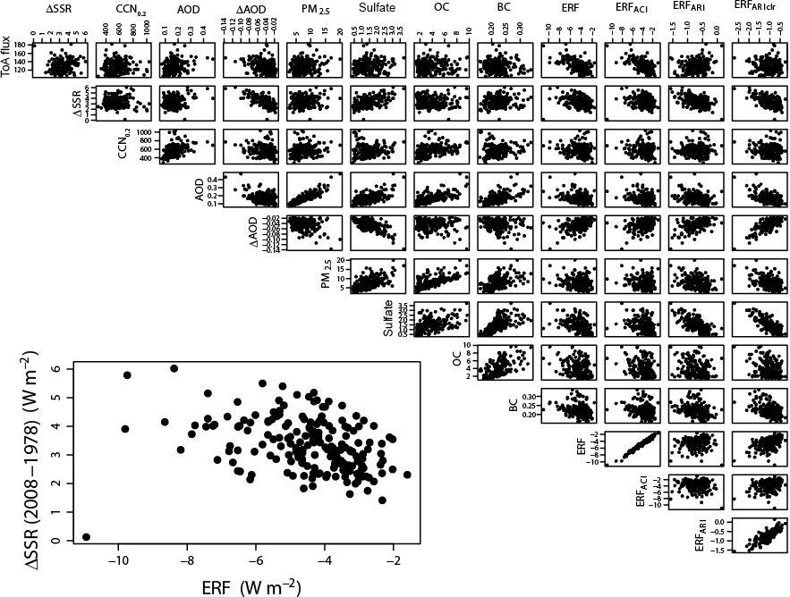
Figure 2Pairwise scatter plots of the PPE member regional mean model output for Europe in July, for the aerosol properties used as constraints: ToA flux (W m−2); change in SSR (ΔSSR, W m−2) between 1978 and 2008; CCN0.2 concentration (cm−3); AOD; surface mass concentrations of PM2.5, sulfate, OC and BC (µg m−3); the change in AOD (ΔAOD, W m−2) between 1978 and 2008; and the 1850–2008 forcing variables: aerosol ERF, ERFACI, ERFARI and ERFARIclr (W m−2).
2.7 Identification of plausible model variants
Observationally plausible model variants are defined to be those that simulate aerosol and radiation properties within the uncertainty ranges of the observations, defined in Table 2. As we use statistical emulators to generate the simulated output values for each model variant, rather than using the climate model directly, an emulator prediction error φ (valued at 1 standard deviation on the emulator prediction from the Gaussian process uncertainty) is also taken into account. Hence for a given observed variable, a model variant is rejected as implausible if the range defined by its emulator prediction ±φ lies outside the corresponding observation's uncertainty range in Table 2. Furthermore, for a joint observational constraint we retain only the model variants that are classed as plausible for all individual observation types that make up the joint constraint. Such a criterion is possible with synthetic observations because we know that the idealized truth is within the model uncertainty space, but the methodology would be more complex if we were using real observations. It is likely that some of the real observations will deviate from the model significantly because of model structural errors and issues related to the representativeness of the observations. Therefore, the use of real observations would necessitate the definition of a measure of plausibility that accounts for known structural and representativeness errors (McNeall et al., 2016; Williamson et al., 2013).
2.8 Aerosol effective radiative forcing (ERF)
We test the effect of observational constraint on the pre-industrial (PI, here 1850) to present-day (PD, 2008) July-mean European aerosol ERF and its components ERFACI (aerosol–cloud interaction) and ERFARI (aerosol–radiation interaction) as well as on the clear-sky component of the ERFARI (ERFARIclr). The ERFs (except the ERFARIclr term) account for above-cloud aerosol scattering and absorption (Ghan, 2013) and are calculated using a fixed sea-surface temperature from 2008.
Table 3Pearson linear correlations (r) between the PPE member regional mean model outputs for Europe in July, for the aerosol properties used as constraints and the 1850–2008 forcing variables, corresponding to the pairwise scatter plots in Fig. 2.
3.1 Relationships among the observed quantities and forcing variables
Figure 2 shows pairwise scatter plots of the PPE member output (European July mean), which provides an overview of the spread of the model outputs as well as the relationships between the variables. We further quantify any linear relationships between the variables using the Pearson correlation coefficient (r) in Table 3.
The aerosol variables show clear inter-relationships. In particular, AOD and PM2.5 concentration show the strongest relationship (Pearson correlation, r=0.88), which is expected given that satellite AOD measurements are frequently used as a proxy for ground-level PM2.5 (Chu et al., 2016). This suggests that AOD and PM2.5 observations will constrain the model uncertainty to a similar extent and therefore only one of these observable quantities is required. AOD and PM2.5 are also clearly correlated with sulfate, OC and BC, which are major components of PM2.5 in polluted regions. CCN0.2 has a relatively weak positive relationship to both AOD (r=0.46) and PM2.5 (r=0.21). A positive correlation is expected because, in general, greater aerosol loading will produce greater CCN0.2 concentrations, but the correlations are weak because the model aerosol size distribution (which determines CCN0.2) can be configured in many different ways to produce the same AOD. The weak AOD–CCN0.2 relation has implications for model constraint: for example, AOD values in the range 0.15–0.2 encompass CCN0.2 concentrations of around 400 to around 1000 cm−3. These results are similar to those of Stier (2016) who showed similarly weak CCN–AOD correlations.
There are clear relationships between industrial-period forcing variables and some of the observable aerosol properties. For ERFARI and ERFARIclr the strongest relationships are with the sulfate concentration ( for ERFARIclr and −0.67 for ERFARI) and multi-decadal ΔAOD (r=0.76 for ERFARIclr and 0.55 for ERFARI). As expected, a present-day higher sulfate concentration corresponds to a stronger (more negative) ERFARI. ΔAOD is negative over Europe due to the reductions in anthropogenic aerosol emissions. Parameter settings that produce a strong multi-decadal ΔAOD also tend to produce a strong pre-industrial to present-day ERFARIclr and therefore a stronger ERFARI. Based on these relationships, uncertainty in ERFARIclr would be easier to constrain than uncertainty in ERFARI and the most useful aerosol observation for this purpose would be European-mean atmospheric sulfate concentration.
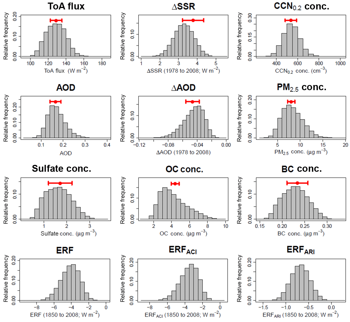
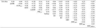
Figure 3Calculated uncertainty in the aerosol quantities and aerosol ERF terms from the 4 million member sample. Results are for the July mean over Europe. The red bar shows the assumed range of each synthetic observation used to constrain the uncertain parameter space and the aerosol forcing uncertainty from Table 2.
For the ERFACI there is a relationship with the reflected shortwave ToA flux (), with a larger flux corresponding to a stronger (more negative) forcing. This relationship means that the parameter settings that produce more reflective aerosols and clouds in the present-day atmosphere also enhance ERFACI forcing. There is also a relationship between the aerosol ERF (pre-industrial to present-day) and the 1978–2008 change in surface shortwave radiation (ΔSSR; ). However, there is a lot of scatter in the relationship because the model parameters that cause uncertainty in decadal radiative changes are similar but not identical to those that cause uncertainty in forcing over the full industrial period (Regayre et al., 2018, 2014). The relationship between ΔSSR and aerosol ERF among seven models was used by Cherian et al. (2014) as an emergent constraint on aerosol ERF over Europe. In Sect. 4 we explore the implications of our uncertainty analysis for such emergent constraint studies.
In summary, the identified relationships in Fig. 2 suggest that for Europe, constraints on sulfate concentration and ΔAOD could lead to some constraint on uncertainty in ERFARI and ERFARIclr. Constraint on ToA flux could lead to some constraint on uncertainty in aerosol ERF and ERFACI over Europe and observed multi-decadal changes in SSR could provide additional constraint. Observational constraints of ERFs are explored in Sect. 3.5.
3.2 Uncertainty in aerosols and radiative forcings
Figure 3 shows probability density functions of the observable aerosol quantities and the ERFs from the Monte Carlo sample of 4 million model variants (Sect. 2.4). These PDFs sample the complete multi-dimensional parameter space of the model, weighted according the prior probability distributions on the input parameters (Yoshioka et al., 2018). The ranges are similar to those in Fig. 2, but the PPE members themselves do not sample the parameter space densely enough to enable a statistically robust PDF to be generated.
The most uncertain observable aerosol properties, with the largest relative standard deviation (ratio of standard deviation to mean value) in our sample are the sulfate and OC concentrations and the multi-decadal ΔAOD (Table 4). This suggests that constraining these properties will substantially reduce the sample size and constrain the parameter space. Some of the PDFs have long tails (e.g. OC concentration and ΔAOD), which suggests that a subset of parameters may be combining in a specific manner to obtain these extreme values. The tails of the forcing PDFs contain the values most likely to be considered implausible against observations (Regayre et al., 2018).
3.3 Sensitivity analysis
We can decompose the overall variance in a model output into percentage contributions from the individual input parameters (Lee et al., 2011; Saltelli et al., 1999). The results of this analysis are shown in Fig. 4.
For many of the output variables there is little correspondence with the forcing variables in terms of the main parameters that cause uncertainty. In particular, only about 10 % of the CCN0.2 concentration uncertainty comes from the main causes of uncertainty in any of the corresponding forcing variables, which is consistent with the weak correlations in Fig. 2 and the conclusions of Lee et al. (2016).
Table 4Mean, standard deviation (σ) and absolute relative standard deviation () of the calculated uncertainty in the aerosol quantities and aerosol ERF terms from the 4 million member sample. Results are for the July mean over Europe.
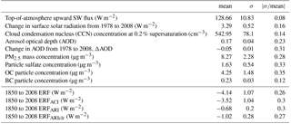
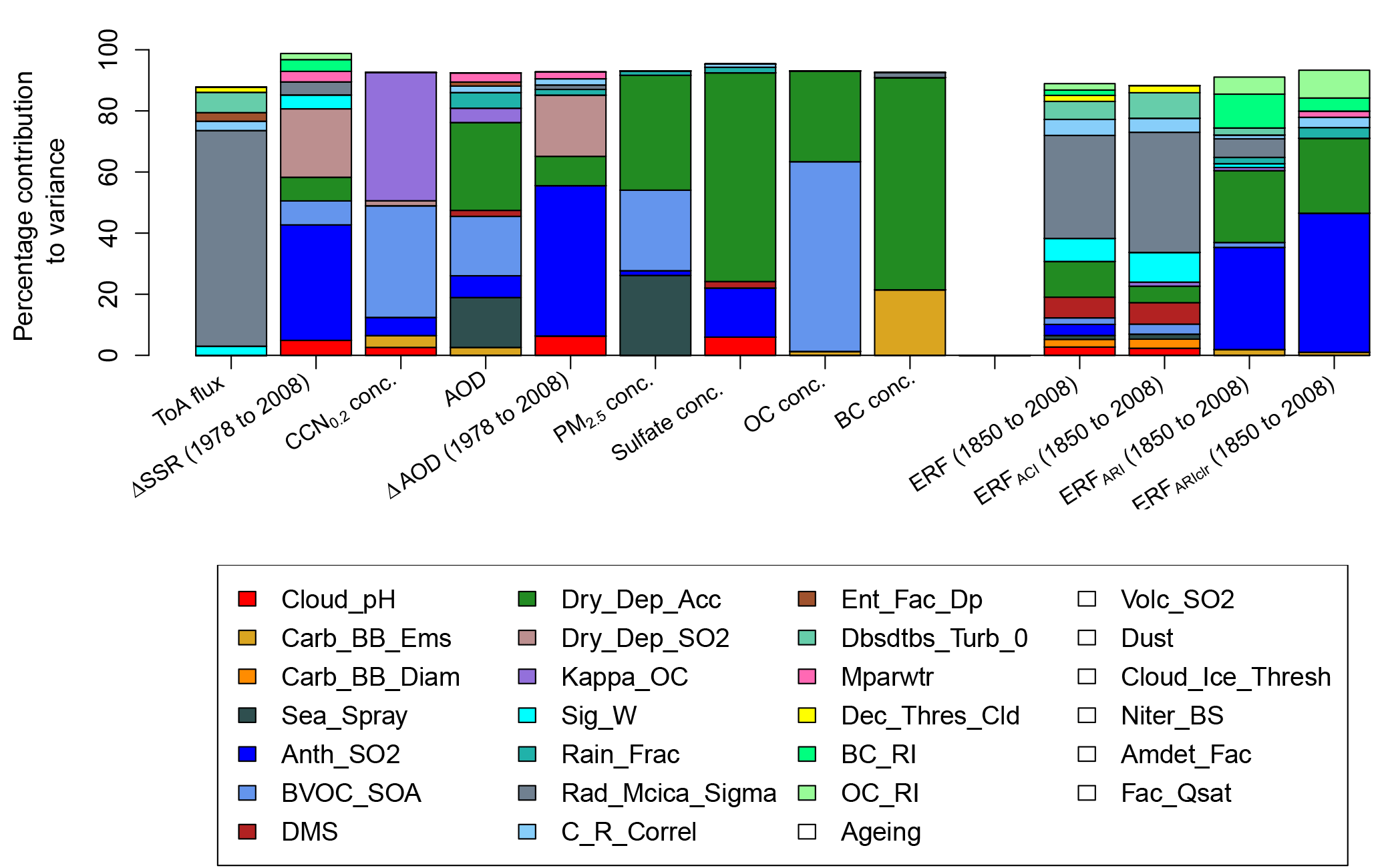
Figure 4Variance-based sensitivity analysis results, showing the percentage parameter contributions to model output uncertainty in the observable aerosol quantities and the forcing variables for Europe in July. Only those parameters which cause at least 1 % of the variance are shown in colour.
There is reasonable correspondence between the sources of uncertainty in sulfate concentration, ΔAOD, ERFARI and ERFARIclr, which is again consistent with Fig. 2. Around 60–70 % of the output variance in these variables is accounted for by anthropogenic SO2 emissions (Anth_SO2) and the accumulation mode dry deposition velocity (Dry_Dep_Acc). This degree of similarity in the parametric uncertainty sources implies that an individual observational constraint on ΔAOD should lead to some constraint of the ERFARI and ERFARIclr forcing uncertainty. Dry_Dep_Acc is also a significant cause of uncertainty in AOD, PM2.5 and concentrations of sulfate, OC and BC (between ∼25 and ∼70 % for each). Hence, it is possible that constraint of these observable aerosol quantities may lead to some constraint on ERFARI and ERFARIclr uncertainty. We also see that the uncertainty in the ToA flux is dominated by the cloud radiation parameter Rad_Mcica_Sigma (which affects the spatial homogeneity of the clouds), which also accounts for about 35 % of the variance in ERF and ERFACI. This parameter also causes most of the uncertainty in global mean ERF and ToA flux (Regayre et al., 2018). However, over Europe in July there are multiple other parameters causing a small amount of the aerosol ERF uncertainty, which suggests an effective constraint will require the use of multiple complementary observations.
3.4 Constraint of aerosol properties
We first explore how constraining an individual aerosol property helps to constrain the range of other observable properties and multi-decadal trends. AOD is the aerosol property most frequently observed and used to evaluate and constrain models (e.g. Shindell et al., 2013) and is used as the control variable in data assimilation used to evaluate the aerosol forcing (Bellouin et al., 2013). Figure 5 shows the reduction in uncertainty of the modelled atmospheric properties and trends by constraining the model to match observed AOD. Credible intervals (95 %) corresponding to the individual constraints are provided in Table 5.
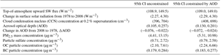
Constraint of July European monthly-mean AOD to lie in the range 0.14–0.19 (23 % of the full ensemble range) leads to a fairly strong constraint of PM2.5 uncertainty: the standard deviation of PM2.5 (σPM2.5) is reduced by 34 % when the range of AOD is reduced by about 77 %. The standard deviation of the PM components and the multi-decadal trend ΔAOD are also reduced, but by a smaller amount: around 20 % for OC and only around 10 % for BC, sulfate and ΔAOD. Constraint of individual chemical components is weaker because there are many combinations of sulfate, BC and OC that can account for high or low AOD. Uncertainty in the other observable quantities (CCN0.2 and ToA flux and the multi-decadal trend ΔSSR) are essentially unaffected by the constraint of AOD. The reason for the weak constraint is that there are many model variants within the observed range of AOD (or PM2.5) that produce very different CCN0.2, ToA flux and ΔSSR.
These results provide some indication of the possible remaining uncertainty in a model that has been tuned to agree with AOD observations. A tuned model that agrees with AOD observations within the observational uncertainty is just one of many potential variants of the model that have equally good agreement with the observations. For example, our model suggests that the remaining uncertainty (absolute range) in July European-mean CCN0.2 concentration could be 755 cm−3 in a model constrained by AOD observations, which is only slightly less than the unconstrained range of 782 cm−3. Most surprisingly, constraint of AOD leaves open a wide range of potential values of the change in AOD over decadal periods. The range of the July ΔAOD from 1978 to 2008 after constraint of 2008 AOD is 0.105 (from −0.109 to −0.004), which is only slightly lower than the unconstrained range of 0.115. Screening model variants based on their ability to reproduce a single aerosol-related observation is not a sufficient constraint on aerosol-related model uncertainty. Therefore tuning a model to AOD observations is completely inadequate for producing a robust aerosol model.
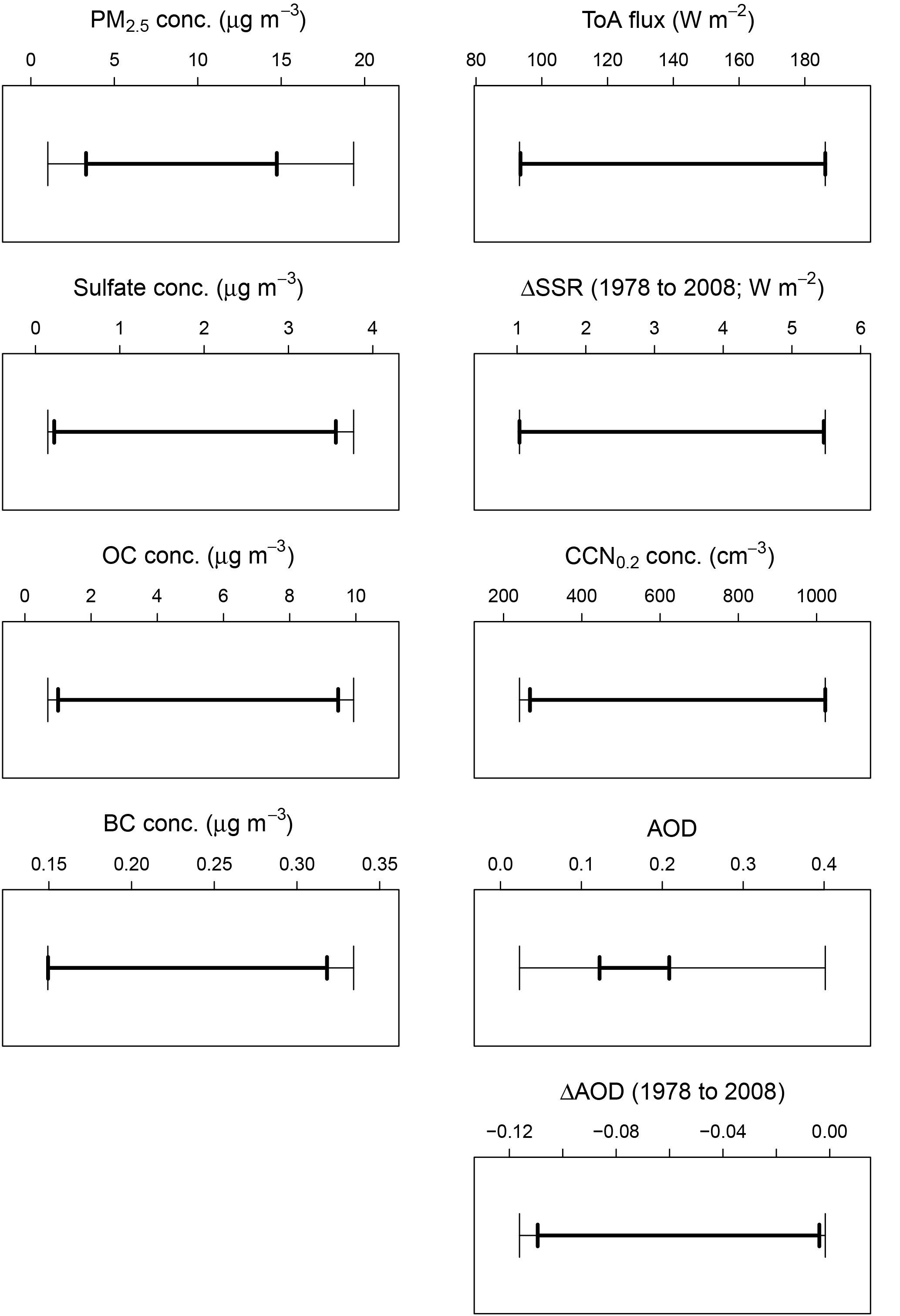
Figure 5Effect of observational constraint of AOD on other aerosol properties in the model over Europe. The bars show the absolute range of the PDF before (thin line) and after (thick line) constraint. Results are for mean properties over Europe in July.
Table 5Effect on the uncertainty in aerosol properties over Europe in July when the model is constrained by AOD (assumed measurement uncertainty range 0.14–0.19). The aerosol uncertainties are given as the 2.5th and 97.5th empirical percentiles of the PDF to form a 95 % credible interval.
3.5 Constraint of 1850–2008 aerosol ERF uncertainty
3.5.1 Effects of individual aerosol and radiation observational constraints
Figure 6a–d show the potential constraint achievable on uncertainty in the July 1850–2008 aerosol ERF, ERFACI, ERFARI and ERFARIclr when we constrain July-mean AOD over Europe. Each box and whisker plot shows the uncertainty distribution from the original sample of 4 million model variants (grey, left) and the sample of constrained models (pink, right). Table 6 shows means and standard deviations for the original and constrained distributions from AOD and all other individual observational constraints.
Observational constraint of simulated AOD has essentially no effect on the range of aerosol ERF and the ERFACI component of forcing over Europe. There is some reduction in uncertainty in the ERFARIclr component of forcing (standard deviation reduced by around 12 %) but not in ERFARI, despite both sharing common causes of uncertainty with AOD (Sect. 3.3).
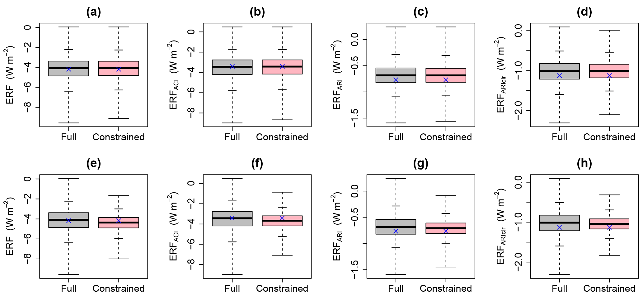
Figure 6The effect of the AOD constraint (a–d) and all observational constraints together (e–h) on the uncertainty in the 1850–2008 forcing variables over Europe in July. Columns left to right show constraint of aerosol ERF, ERFACI, ERFARI and ERFARIclr (W m−2). The boxes show the interquartile range (with the median value shown by the black line that cuts it) and the whiskers show the full range of the distribution. The short horizontal bars on the whiskers correspond to 95 % credible interval bounds. The grey boxes show the distribution for the variable predicted over the original sample (4 million model variants that span the underlying parameter uncertainty) and the pink boxes show the corresponding distribution of the remaining samples after the constraint has been applied. The predicted forcing using the input combination of the model run used as the idealized observation is shown by the blue cross.
Table 6Mean and standard deviation (in brackets) of the forcing distributions over Europe in July for the original unconstrained sample, the multiple-constraint sample and the individually constrained samples where each observational constraint is applied independently.
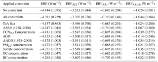
Figure 7 summarizes the effect of the other individual constraints. For ERFACI (and therefore aerosol ERF, which is dominated by ERFACI) the only observation that has any meaningful effect on the range is the ToA flux. When the flux is constrained to be within the range 122–135 W m−2 (from the prior range of 90–175 W m−2), the standard deviation of ERFACI over Europe in July falls by 24 % (Table 6). The ΔSSR observation reduces the aerosol ERF and ERFACI standard deviations by less than 3 %. The only other constraints on uncertainty in aerosol ERF and ERFACI come from constraining AOD or ΔAOD, which reduce the forcing uncertainties by around 3 % each. The effect of applying all observations in combination is discussed in Sect. 3.5.2.
ERFARI and ERFARIclr are constrained by several individually applied observations. ΔAOD and sulfate concentrations provide the strongest constraints. ΔAOD reduces the standard deviation of ERFARI and ERFARIclr by 14 % and 24 % respectively. Constraining sulfate concentrations reduces the uncertainty in ERFARI by 18 % and in ERFARIclr by 21 %. The strong constraint of ERFARI and ERFARIclr uncertainty is consistent with Fig. 4, where we saw that around 60–70 % of the uncertainty in ΔAOD, ERFARI and ERFARIclr could be attributed to the same two parameters. Again, the relatively weak constraint is caused by interacting combinations of parameter effects (Lee et al., 2016; Regayre et al., 2018; Sect. 3.7), so there is potential for significant error compensation (or equifinality, Beven and Freer, 2001). In all other cases the individual observational constraints reduce the uncertainty in ERFARI and ERFARIclr by less than 10 %.

Figure 7The relative constraint achieved for aerosol ERF, ERFACI, ERFARI and ERFARIclr over Europe in July given the individual synthetic constraints applied (colours) and the simultaneous constraint (ALL). The relative constraint is evaluated as (a) the ratio of the standard deviation of the forcing in the constrained sample (σconstrained) to the standard deviation of the forcing in the original, unconstrained sample (σfull); (b) the ratio of the constrained forcing range (rangeconstrained) to the unconstrained forcing range (rangefull).
3.5.2 Effect of all observational constraints
Figure 6e–h and the right-most bars in Fig. 7 show the reduction in July European-mean 1850–2008 aerosol ERF, ERFACI, ERFARI and ERFARIclr uncertainty when we simultaneously apply all nine observational constraints. The standard deviations are reduced by 29.4 % for the aerosol ERF, 29.5 % for ERFACI, 27.8 % for ERFARI and 34.3 % for ERFARIclr (Table 6) and Fig. 6 shows a reduction in the interquartile range (box width) and 95 % credible interval in each case.
Our results show that multiple observational constraints are very effective at reducing the plausible parameter space (ruling out 96.4 % of model variants). However, these reductions in parameter space have only a modest impact on aerosol ERF uncertainty. This occurs because the 27 parameter values in the constrained space can be combined to produce a wide range of ERFs (Lee et al., 2016). These results highlight the value of exploring the wider underlying modelling uncertainties (achieved here using a well-designed PPE to inform statistical emulation). The more comprehensive exploration of the parameter space using several million model variants from the emulators enabled us to explore the wider uncertainties that would not have been captured even by the 191 PPE members. Furthermore, a 96.4 % reduction in parameter space would have reduced the number of PPE members to one or two, which would not have revealed that a large fraction of the ERF uncertainty (70.6 %) remained unconstrained. Likewise, a single model variant arrived at through tuning cannot represent model behaviour over the remaining plausible parameter space. Similar concerns about non-robust samples apply also to the small number of members in multi-model ensembles.
3.5.3 Effect of combinations of observational constraints
An important question in model constraint is how quickly the model uncertainty falls as additional observational constraints are applied. Figure 8 shows the average reduction in forcing uncertainty versus the number of observational constraints applied. With 9 possible observational constraints there are 9 possible single constraints, 36 possible combinations of 2 constraints, 252 combinations of 3 constraints, etc. We therefore show a mean over all possible combinations of each number of constraints.
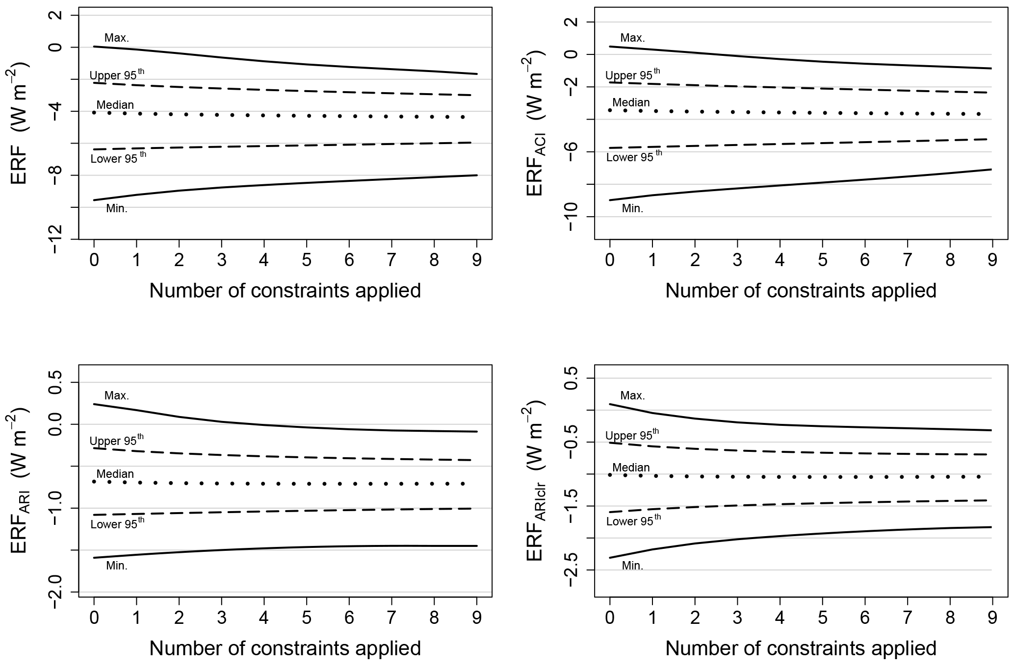
Figure 8The dependence of July aerosol ERF uncertainty on the number of observational constraints applied. The lines show the mean effect of different numbers of constraints.
Averaged across the many combinations of constraints, uncertainty in aerosol ERF and its components initially falls approximately linearly with the number of constraints applied, but then flattens out. This dependence implies that some observations are constraining the same sources of uncertainty as other observations (as shown in Sect. 3.3). So while a large number of observations are needed to constrain forcing, it is also important to identify observations that provide unique constraints on parameter uncertainties. The effectiveness of each observational constraint depends on which other constraints are applied with it. For example, two positively correlated observations like PM2.5 and AOD (Fig. 2) will reduce the allowable parameter space in broadly the same dimensions because the same parameters cause their uncertainty (Fig. 4). Therefore the constraint on forcing uncertainty achieved by AOD and PM2.5 is not additive.
3.6 Constraint of 1978–2008 forcing uncertainty
Previous research has shown that the causes of uncertainty in recent decadal forcing are quite different to the causes of uncertainty in pre-industrial to present-day forcing (Regayre et al., 2018, 2014). Much of the uncertainty in PI to PD aerosol–cloud interaction forcing is caused by natural aerosols (Carslaw et al., 2013, 2017), which are much less important over recent decades. We therefore expect recent aerosol and radiation observations to provide a greater constraint on recent decadal forcings than on forcing referenced to PI conditions. Our results show that this hypothesis is correct: simultaneous application of the nine observational constraints reduces the standard deviation of the July 1978–2008 aerosol forcing distributions by 33.7 % for ERF, 32.3 % for ERFACI, 35.0 % for ERFARI and 43.9 % for ERFARIclr, which are all greater reductions than for the 1850 to 2008 forcing (Fig. 7, Table 6). The main contributor to the reduction in uncertainty in the aerosol ERF from 1978 to 2008 is the change in AOD, followed by present-day AOD. These results suggest that forcing uncertainty in recent decades may be more readily constrained by observations than multi-century forcing.
3.7 Constraint of plausible parameter ranges
The overall objective of our approach is to identify all the observationally plausible variants of the model so that they can be used to calculate an observationally constrained spread of aerosol ERFs. Each variant is associated with a particular part of parameter space. We can therefore use the emulators to compute the constrained magnitude and range of any other aerosol property (or the changes between 1850, 1978 and 2008). Alternatively a sample of these variants (parameter settings) could be used in the model itself to simulate aerosol effects for any situation (for example, with very different meteorological conditions, or anthropogenic aerosol emissions).
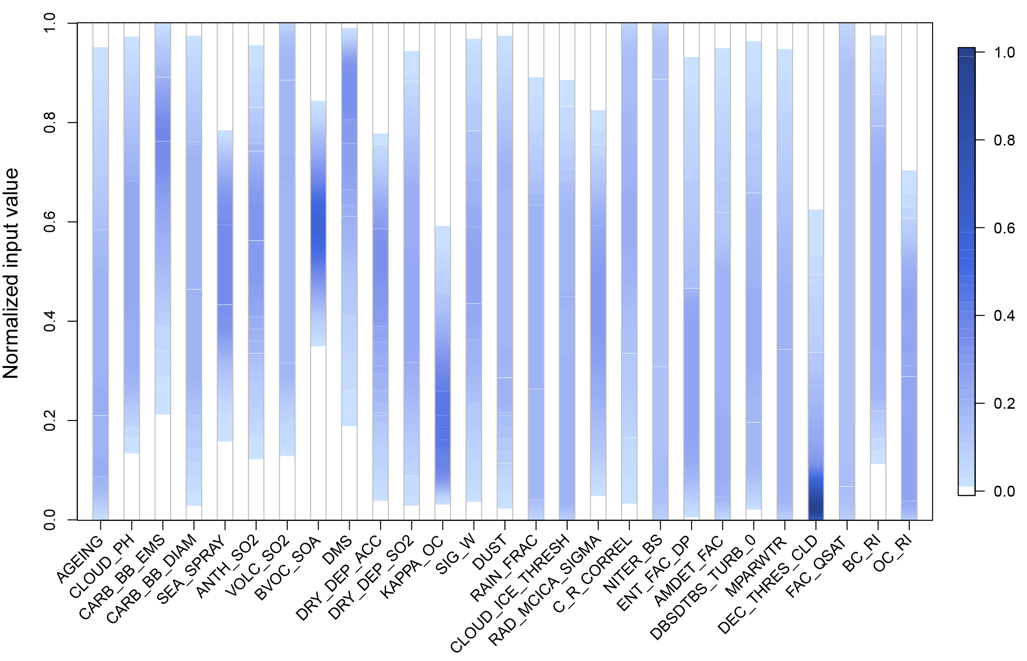
Figure 9One-dimensional projection of the remaining parameter space after simultaneous constraint of all atmospheric quantities and decadal trends. The colour-scale shows the marginal normalized sampling density (normalized across parameters) of each input parameter over its range. Parts of the marginal parameter space that are effectively ruled out are shown in white (normalized sampling density <0.02).
Figure 9 shows a one-dimensional projection of the remaining parameter space after constraining to the nine observations. There are some substantial reductions in the plausible marginal range of several individual parameters. It needs to be borne in mind that, with 27 parameter dimensions, the parameter relationships which have been constrained by multiple observations cannot be seen in the one-dimensional projection. That is, the remaining plausible individual parameter values can be combined in many ways with the remaining space of the other parameters and still reproduce all of the observations (Lee et al., 2016; Regayre et al., 2018). Figure 9 identifies parts of the marginal parameter space that are effectively ruled out in white. For example, a very low setting of the BVOC_SOA parameter cannot produce observationally plausible results when combined with any of the possible combinations of the other 26 parameters.
The constraint of the parameter ranges will be different when using real observations, but it is interesting to see how nine observations can marginally constrain 27 parameters when there is a high degree of potentially compensating effects. The strongest marginal constraint is on the following: the sea spray aerosol emissions (Sea_Spray; the highest 25 % and lowest 15 % of values are implausible), biogenic secondary aerosol formation (BVOC_SOA; the lowest 40 % and top 20 % of the range are implausible), the hygroscopicity of organic carbon (Kappa_OC; the top 40 % of values are implausible) and the imaginary part of organic carbon refractive index (OC_RI; top 30 % is implausible). Furthermore, the lowest 10 %–20 % of the range of several aerosol emission parameters are also deemed implausible – biomass burning (Carb_BB_Ems), degassing volcanic (Volc_SO2), DMS, anthropogenic sulfur dioxide (Anth_SO2).
The atmospheric (host model) marginal parameter ranges are much less constrained because the observable variables that we used are not strongly dependent on them, except for ToA flux observations, which are known to be affected by the Dec_Thresh_Cld and Rad_Mcica_Sigma parameters (Regayre et al., 2018). Values of the threshold for cloudy boundary layer decoupling parameter (Dec_Thresh_Cld) are concentrated towards the lower end of the range (the upper 40 % are implausible). We also show that the top 20 % of values are implausible for the parameter controlling the amount of overlap between sub-grid clouds as seen by the model's radiation code (Rad_Mcica_Sigma). However, the lowest 40 % of this parameter range can be entirely ruled out by constraining the ToA flux in the North Pacific (Regayre et al., 2018). These results highlight the important benefits which will come from constraining the model uncertainty using multiple observations in multiple environments.
This analysis highlights the complexity of the multi-dimensional parameter uncertainty space that remains after observational constraint: there are clearly a large number of ways of tuning a model to be observationally plausible.
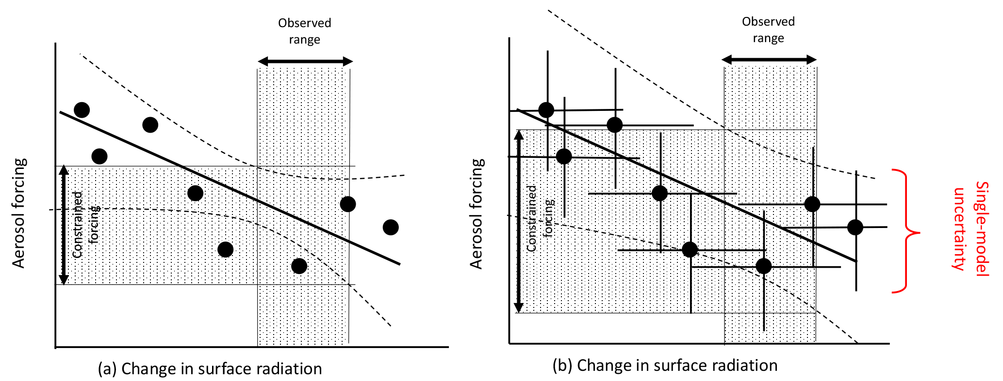
Figure 10An example of an emergent constraint of the aerosol forcing using results from multiple models. (a) A relatively tight apparent constraint when the uncertainty in the individual models is neglected; (b) a much weaker constraint when the uncertainty in the individual models is accounted for.
In multi-model ensembles it is usually the case that each modelling group submits a single well-tuned version (variant) of a model. The uncertainty in the ensemble is determined by the structural differences between the models, but the uncertainty in the individual models (caused by multiple uncertain parameter settings) is not quantified. Here we use the uncertainty in HadGEM3-UKCA to estimate the effect it might have on the results of multi-model emergent constraint studies. Clearly the uncertainties in each model will differ, so we use our model uncertainty only as a rough estimate of the potential effect.
In the ACCMIP study (Shindell et al., 2013), model skill at simulating AOD was used to screen nine models. We have described in Sect. 3.4 and 3.5 why constraint of AOD can only be considered the first step in model screening; AOD does not effectively reduce model uncertainty when used in isolation. The standard deviation of the modelled global annual mean ERFARI in the ACCMIP study was about 50 % of the multi-model mean. In our results, after we have screened out model variants that are inconsistent with synthetic AOD observations (i.e. effectively tuning to AOD), the standard deviation of the HadGEM-UKCA ERFARI over Europe in July is about 30 % of our mean. Therefore the standard deviation in HadGEM3-UKCA caused by uncertain input parameters is a significant fraction of the multi-model standard deviation, and would affect the constrained range of ERFARI. Shindell et al. (2013) acknowledged that uncertainties in the emissions could alter the relative agreement of the models with observations and thereby affect the spread of plausible model predictions. However, uncertainty in emissions is just one of many possible sources of uncertainty that could affect the conclusions (Fig. 4).
In emergent constraint studies a linear relationship between aerosol forcing and an observable variable simulated by multiple models is used to define an observationally constrained value of the variable of interest. In the Cherian et al. (2014) study European-mean aerosol ERF was estimated by regressing modelled ERF against the 1990–2005 modelled trend in SSR over Europe from seven aerosol–climate models. An observed SSR trend of W m−2 decade−1 enabled the European-mean aerosol ERF to be constrained to W m−2 (corresponding to the range of −4.97 to −2.15 W m−2). Their analysis accounted for the uncertainty in SSR caused by meteorological variability but did not account for the influence of parametric uncertainties.
In our HadGEM3-UKCA simulations the July European-mean aerosol ERF 95 % credible interval is −6.0 to −2.7 W m−2 after constraining the model using nine observations (i.e. a tight tuning of the model). This range provides some measure of the range of alternative ERFs that could be obtained by the individual models had they been tuned differently (but equally well) to observations (although we do not know what actual tuning was undertaken). Our single-model uncertainty range is comparable to the multi-model ensemble range, but was not accounted for by Cherian et al. (2014) in deriving the emergent constraint. The effect of including this previously neglected source of single-model uncertainty is to substantially increase the uncertainty on the emergent constraint (Fig. 10). Furthermore, the likely magnitude of forcing derived from emergent constraints is sensitive to the uncertainties accounted for in the process (Samset et al., 2014).
In many emergent constraint studies, the constrained ERF (or other quantity) is essentially based on the very small number of models that lie within the uncertainty range of one observation (Fig. 10). With our approach, model variants that are plausible against this one observation type are then examined to determine their plausibility against many other observation types – in this study, nine observations in total. Ultimately, multivariate constraint is essential to reach robust conclusions because of the many compensating sources of model uncertainty.
The use of observations to produce a well-configured model variant is a fundamental aspect of ensuring that models can make trustworthy predictions. For example, in a review of progress on reducing uncertainty in direct radiative forcing, Kahn (2012) argues that models can be “constrained by the aggregate of observational data, to calculate the regional and global radiation fields and material fluxes with adequate space–time resolution to produce the best result we can achieve”. The primary objective of our study was to determine how much uncertainty could remain in an aerosol–climate model when it is constrained to match combinations of observations that define the base state of the model: top-of-atmosphere upward shortwave flux, aerosol optical depth, PM2.5, cloud condensation nuclei at 0.2 % supersaturation, concentrations of sulfate, black carbon and organic material as well as multi-decadal change in surface shortwave radiation and aerosol optical depth. Our results refer to July-mean conditions over Europe.
To estimate the uncertainty that might typically exist in a climate model before and after tuning, we used a perturbed parameter ensemble that sampled uncertainties in 27 parameters related to aerosol emissions, aerosol and cloud processes, and parameters in the host physical climate model that influence clouds, humidity, convection and radiation in the base state of the model. We performed 191 model simulations that spanned the 27-dimensional space of the model uncertainty and then built surrogate model emulators from which we created a Monte Carlo sample of 4 million “model variants”. Using synthetic observations (taken from the output of one of our simulations) we determine the extent of the potential constraint that the nine aerosol and cloud-related properties can generate. Constraining the model outputs using all nine observations rules out over 96 % of the model variants and the associated implausible parts of parameter space. The remaining 153 000 model variants have been used to estimate the observationally constrained aerosol ERF and the uncertainty associated with one tuned version of HadGEM3-UKCA.
Tuning HadGEM3-UKCA to AOD alone has almost no effect on the reliability of the tuned model to simulate CCN0.2 (and hence cloud drop number concentrations) (Fig. 5). Constraining European-mean AOD in July to lie within a realistic range of 0.14–0.19 (23 % of the full model uncertainty range) results in a reduction of less than 5 % in the uncertainty in CCN0.2 generated by the full set of 4 million variants of the model. The CCN0.2 concentration range is then 268–1022 cm−3 compared to 241–1022 cm−3. This provides a measure of the parametric uncertainty when AOD measurements are used to infer CCN, although the range would potentially be larger had we perturbed more parameters (Yoshioka et al., 2018). Tuning a model to AOD alone also has very little effect on the modelled range of the trend in AOD over a multi-decadal period. The complete set of model variants produces a range of changes in AOD over Europe in July of 0.115 for the years 1978 to 2008, and this range is only reduced to 0.105 (from −0.109 to 0.004) when the model is constrained to match July European-mean 2008 AOD within observational uncertainty.
Constraint of AOD alone has a negligible effect on the uncertainty in the aerosol ERF over Europe in July. Although the aerosol ERF simulated by a model will change as parameters are tuned to achieve agreement with AOD measurements, any resulting ERF will have large uncertainty (i.e. there are many other equally well-tuned model variants that produce different ERFs). This uncertainty cannot easily be estimated without a full uncertainty analysis of the model as we have done here. The weak constraint calls into question the robustness of estimates of aerosol forcing based on AOD reanalyses (Bellouin et al., 2013).
It is often argued that AOD is a poor variable to use for understanding aerosol–cloud interactions. However, our results show that even the most strongly related measurement (CCN0.2) does not provide a strong individual constraint on ERFACI either (Fig. 7). It is doubtful that other derived variables like aerosol index will be any better. The key to model constraint is to find combinations of observations that help to constrain ERF: Individual constraints are unlikely to be effective, although they may appear to be effective if the model uncertainty is not fully sampled.
Observational constraint using nine observations has the potential to reduce the uncertainty in aerosol ERF slightly more over a multi-decadal period than over the full industrial period: the standard deviation falls by 29.4 % for the July 1850–2008 aerosol ERF, 29.5 % for ERFACI, 27.8 % for ERFARI and 34.3 % for ERFARIclr. The standard deviation of 1978–2008 aerosol ERF in July could be reduced by around 34 %, which is greater than for the 1850–2008 ERF because there is greater correspondence between the causes of uncertainty in near-term aerosol forcing and the 2008 aerosol–cloud–radiation state than there is between the 1850–2008 ERF and the 2008 state (Regayre et al., 2018, 2014). Because near-term future changes in aerosols and clouds are likely to resemble recent changes more than centennial-scale changes, we are optimistic that the uncertainty in near-term aerosol ERFs could be constrained and used to provide policy-relevant information on near-term temperature changes (Hawkins et al., 2017). A shift of emphasis of the research community towards trying to constrain decadal forcing uncertainty, instead of industrial era forcing, is likely to accelerate progress.
The most effective observational constraint on the uncertainty in aerosol ERF and ERFACI is the top-of-atmosphere upward shortwave flux. When the flux for July is constrained to be within the range 122–135 W m−2 (from the prior range of 90–175 W m−2) the standard deviation of ERFACI over Europe in July falls by 24 %. Other observational constraints reduce the ERFACI uncertainty by a few percent at most, including the change in surface SW radiation. Effectively, this result means that routine tuning of radiative fluxes in climate models will have a bearing on the magnitude of the aerosol ERF that the models calculate. The reason for the constraint on forcing uncertainty is that model parameters that control cloud and atmosphere brightness also control how that brightness responds to changes in aerosols over Europe. However, it is only likely to be an effective constraint where the brightness is controlled by tuning the parameters we have identified here. In regions dominated by quite different processes, like mixed-phase clouds, tuning the flux will have a much weaker effect on the aerosol ERF.
The most effective observational constraints on the uncertainty in July ERFARI and ERFARIclr over Europe are the sulfate concentration and the change in AOD over a multi-decadal period (we used 1978–2008). When applied individually, sulfate concentrations constrain ERFARI standard deviation in our ensemble by 18 % over Europe in July. The 1978–2008 change in AOD constrains the ERFARI standard deviation by 14 % when applied individually. Constraint of AOD itself (in 2008) reduces the ERFARI uncertainty by only 5 %, and would not provide a realistic way of screening models. The other constraints were much less effective.
The plausible ranges of some natural aerosol emissions are reduced after constraining to the nine observations, particularly sea spray emissions and biogenic volatile organic aerosol formation. We were also able to constrain some aerosol process parameters such as the CCN hygroscopicity (kappa), the imaginary refractive indices of BC and OC, and parameters controlling boundary layer stability and the radiative properties of overlapping sub-grid clouds which control cloud brightness. Observational constraint generates a set of constrained parameter settings that can be taken forward and used to make model predictions under any other conditions (e.g. for future projections).
The range and combinations of observationally plausible parameter values remain very large even after constraint using nine observations, which explains why the aerosol ERF uncertainty remains large after constraint. This result is not a failure of our approach, but rather an indication of the multiple ways in which uncertain model parameters can combine to predict a wide range of outputs with equal skill when compared to observations. These multiple model variants are neglected when a single model variant is produced through tuning.
Widely used procedures of aerosol–climate model evaluation and observational “validation” lack statistical robustness because they do not adequately sample the model uncertainty space. We showed that observational constraint against nine observations identified less than 4 % of the 4 million sampled points in multi-dimensional parameter space as plausible (i.e. the model value is within the observational uncertainty). A 96 % reduction in parameter space would have reduced our original set of 191 ensemble members to one or two, which would not have revealed that a large fraction of the ERF uncertainty (about 71 %) remained unconstrained. This creates a fundamental problem for multi-model ensembles (which have far fewer members) and model tuning (which may explore only a few dozen model variants and mostly with single parameter perturbations). From such small samples of models it is not possible to determine how observations help to reduce model uncertainty, so estimates of radiative forcing should not be considered robust.
Our results have implications for studies that seek emergent constraints on a small set of models based on one observational metric. An emergent constraint can be informative, but cannot be expected to reduce the uncertainty in a complex model when used in isolation. The example closest to our study is Cherian et al. (2014), in which the relationship between aerosol ERF and the trend in surface solar radiation (SSR) over Europe for seven climate models was used to estimate the observationally constrained uncertainty in aerosol ERF. Our results for the HadGEM3-UKCA model show that the uncertainty in aerosol ERF and SSR trends in any one tuned version of the model is likely to be of the same order of magnitude as the multi-model range. If the uncertainties in individual models in an ensemble are not accounted for, then we risk being over-confident in the emergent constraints. Efforts to quantify and observationally constrain individual models are therefore not an alternative to multi-model studies, but individual model uncertainty needs to be quantified and incorporated as an essential component of such efforts to understand and then reduce aerosol ERF uncertainty.
There is considerable scope to extend our approach to incorporate more observation types and more regions. These should include the following: (1) aerosol and radiation trends (Allen et al., 2013; Cherian et al., 2014; Leibensperger et al., 2012; Li et al., 2013; Liepert and Tegen, 2002; Shindell et al., 2013; Turnock et al., 2015; Zhang et al., 2017) – so far we used changes in AOD and SSR, but changes in ToA SW flux as well as aerosol components like OC (Ridley et al., 2018) and sulfate could provide useful constraints; (2) observations from pristine regions that might provide a constraint on pre-industrial-like aerosol and cloud properties (Carslaw et al., 2017; Hamilton et al., 2014); (3) information on the vertical profile of aerosols; and (4) observed relationships between changes in aerosol and cloud variables (Ghan et al., 2016; Gryspeerdt et al., 2017; Quaas et al., 2009) such as defined in Eq. (1). Such relationships are a favoured way to constrain forcing. Although it is conceivable that relationships between change-of-state variables can be predicted more reliably than state variables themselves (because of cancellation of correlated model errors), the model uncertainty in these relationships has not been determined in studies that have applied them.
Whichever approach is used to reduce uncertainty in aerosol forcing, it is essential to acknowledge that aerosol–chemistry–climate models are highly complex with dozens of sources of uncertainty that can be combined in many ways. Such a system cannot be constrained by one or two observations at a time, and emergent constraints are no different in this respect. Robust constraint of a high-dimensional system requires large numbers of combined constraints so that the multiple compensating dimensions of uncertainty can be reduced (Reddington et al., 2017). We are reasonably confident that extension of our approach to more and varied observations will enable the uncertainty in aerosol radiative forcing to be reduced significantly.
Data can be made available upon request from the corresponding author. The authors welcome use of the perturbed parameter ensemble for advancing climate research.
JSJ applied the statistical methodology and generated and analysed the results. JSJ, LAR and KSC wrote the article. All authors contributed to the analysis and interpretation of results. KJP, MY, LAR, KSC and JSJ helped prepare the model configuration that served as the template for the PPE. LAR and JSJ designed the experiments. All PPE simulations were created by LAR. MY advised on computational aspects of the ensemble creation. The screening of atmospheric parameters was conducted by LAR, DMHS and KSC. LAR and JSJ elicited probability density functions of all aerosol parameters, and KSC, KJP, MY and LAL participated (alongside many other experts) in the formal elicitation process.
The authors declare that they have no conflict of interest.
This research was funded by the Natural Environment Research Council (NERC)
under grants NE/J024252/1 (GASSP), NE/I020059/1 (ACID-PRUF) and NE/P013406/1
(A-CURE); the European Union ACTRIS-2 project under grant 262254; the
National Centre for Atmospheric Science (Yoshioka, Carslaw); and the
UK–China Research and Innovation Partnership Fund through the Met Office
Climate Science for Service Partnership (CSSP) China as part of the Newton
Fund. We made use of the N8 HPC facility funded from the N8 consortium and an
Engineering and Physical Sciences Research Council Grant to use ARCHER
(EP/K000225/1) and the JASMIN facility (http://www.jasmin.ac.uk/, last
access: 4 September 2018) via the Centre for Environmental Data Analysis,
funded by NERC and the UK Space Agency and delivered by the Science and
Technology Facilities Council. We acknowledge the following additional
funding: the Royal Society Wolfson Merit Award (Kenneth S. Carslaw), a
doctoral training grant from the Natural Environment Research Council and a
CASE studentship with the Met Office Hadley Centre
(Leighton A. Regayre).
Edited by: Patrick
Chuang
Reviewed by: Johannes Mülmenstädt and two
anonymous referees
Allen, R. J., Norris, J. R., and Wild, M.: Evaluation of multidecadal variability in CMIP5 surface solar radiation and inferred underestimation of aerosol direct effects over Europe, China, Japan, and India, J. Geophys. Res.-Atmos., 118, 6311–6336, https://doi.org/10.1002/jgrd.50426, 2013.
Andreae, M. O., Jones, C. D., and Cox, P. M.: Strong present-day aerosol cooling implies a hot future, Nature, 435, 1187–1190, https://doi.org/10.1038/nature03671, 2005.
Andres, R. J. and Kasgnoc, A. D.: A time-averaged inventory of subaerial volcanic sulfur emissions, J. Geophys. Res.-Atmos., 103, 25251–25261, https://doi.org/10.1029/98JD02091, 1998.
Andrianakis, I., Vernon, I., McCreesh, N., McKinley, T. J., Oakley, J. E., Nsubuga, R. N., Goldstein, M., and White, R. G.: History matching of a complex epidemiological model of human immunodeficiency virus transmission by using variance emulation, J. R. Stat. Soc. C-Appl., 66, 717–740, https://doi.org/10.1111/rssc.12198, 2017.
Ban-weiss, G. A., Jin, L., Bauer, S. E., Bennartz, R., Liu, X., Zhang, K., Ming, Y., Guo, H., and Jiang, J. H.: Evaluating clouds, aerosols, and their interactions in three global climate models using satellite simulators and observations, J. Geophys. Res., 119, 10876–10901, https://doi.org/10.1002/2014JD021722, 2014.
Bellouin, N., Quaas, J., Morcrette, J.-J., and Boucher, O.: Estimates of aerosol radiative forcing from the MACC re-analysis, Atmos. Chem. Phys., 13, 2045–2062, https://doi.org/10.5194/acp-13-2045-2013, 2013.
Beven, K. and Freer, J.: Equifinality, data assimilation, and uncertainty estimation in mechanistic modelling of complex environmental systems using the GLUE methodology, J. Hydrol., 249, 11–29, https://doi.org/10.1016/S0022-1694(01)00421-8, 2001.
Boucher, O., Randall, D., Artaxo, P., Bretherton, C., Feingold, G., Forster, P., Kerminen, V.-M., Kondo, Y., Liao, H., Lohmann, U., Rasch, P., Satheesh, S. K., Sherwood, S., Stevens, B., and Zhang, X. Y.: Clouds and Aerosols, in: Climate Change 2013: The Physical Science Basis. Contribution of Working Group I to the Fifth Assessment Report of the Intergovernmental Panel on Climate Change, edited by: Stocker, T. F., Qin, D., Plattner, G.-K., Tignor, M., Allen, S. K., Boschung, J., Nauels, A., Xia, Y., Bex, V., and Midgley, P. M., Cambridge University Press, Cambridge, UK and New York, NY, USA, 571 pp., 2013.
Boutle, I. A., Abel, S. J., Hill, P. G., and Morcrette, C. J.: Spatial variability of liquid cloud and rain: observations and microphysical effects, Q. J. Roy. Meteor. Soc., 140, 583–594, https://doi.org/10.1002/qj.2140, 2014.
Carslaw, K. S., Lee, L. A., Reddington, C. L., Pringle, K. J., Rap, A., Forster, P. M., Mann, G. W., Spracklen, D. V, Woodhouse, M. T., Regayre, L. A., and Pierce, J. R.: Large contribution of natural aerosols to uncertainty in indirect forcing, Nature, 503, 67–71, https://doi.org/10.1038/nature12674, 2013.
Carslaw, K. S., Gordon, H., Hamilton, D. S., Johnson, J. S., Regayre, L. A., Yoshioka, M., and Pringle, K. J.: Aerosols in the Pre-industrial Atmosphere, Curr. Clim. Chang. Reports, 3, 1–15, https://doi.org/10.1007/s40641-017-0061-2, 2017.
Cherian, R., Quaas, J., Salzmann, M., and Wild, M.: Pollution trends over Europe constrain global aerosol forcing as simulated by climate models, Geophys. Res. Lett., 41, 2176–2181, https://doi.org/10.1002/2013GL058715, 2014.
Chu, Y., Liu, Y., Li, X., Liu, Z., Lu, H., Lu, Y., Mao, Z., Chen, X., Li, N., Ren, M., Liu, F., Tian, L., Zhu, Z., and Xiang, H.: A Review on Predicting Ground PM2.5 Concentration Using Satellite Aerosol Optical Depth, Atmosphere, 7, 129, https://doi.org/10.3390/atmos7100129, 2016.
Craig, P. S., Goldstein, M., Seheult, A. H., and Smith, J. A.: Pressure Matching for Hydrocarbon Reservoirs: A Case Study in the Use of Bayes Linear Strategies for Large Computer Experiments, in: Case Studies in Bayesian Statistics, Lecture Notes in Statistics, Vol. 121, edited by: Gatsonis, C., Hodges, J. S., Kass, R. E., McCulloch, R., Rossi, P., and Singpurwalla N. D., Springer, New York, NY, 1997.
Edwards, N. R., Cameron, D., and Rougier, J.: Precalibrating an intermediate complexity climate model, Clim. Dynam., 37, 1469–1482, https://doi.org/10.1007/s00382-010-0921-0, 2011.
Ghan, S., Wang, M., Zhang, S., Ferrachat, S., Gettelman, A., Griesfeller, J., Kipling, Z., Lohmann, U., Morrison, H., Neubauer, D., Partridge, D. G., Stier, P., Takemura, T., Wang, H., and Zhang, K.: Challenges in constraining anthropogenic aerosol effects on cloud radiative forcing using present-day spatiotemporal variability, P. Natl. Acad. Sci. USA, 113, 5804–5811, https://doi.org/10.1073/pnas.1514036113, 2016.
Ghan, S. J.: Technical Note: Estimating aerosol effects on cloud radiative forcing, Atmos. Chem. Phys., 13, 9971–9974, https://doi.org/10.5194/acp-13-9971-2013, 2013.
Ghan, S. J. and Schwartz, S. E.: Aerosol Properties and Processes: A Path from Field and Laboratory Measurements to Global Climate Models, B. Am. Meteorol. Soc., 88, 1059–1083, https://doi.org/10.1175/BAMS-88-7-1059, 2007.
Grandey, B. S., Stier, P., and Wagner, T. M.: Investigating relationships between aerosol optical depth and cloud fraction using satellite, aerosol reanalysis and general circulation model data, Atmos. Chem. Phys., 13, 3177–3184, https://doi.org/10.5194/acp-13-3177-2013, 2013.
Gryspeerdt, E. and Stier, P.: Regime-based analysis of aerosol-cloud interactions, Geophys. Res. Lett., 39, 1–5, https://doi.org/10.1029/2012GL053221, 2012.
Gryspeerdt, E., Quaas, J., and Bellouin, N.: Constraining the aerosol influence on cloud fraction, J. Geophys. Res., 121, 3566–3583, https://doi.org/10.1002/2015JD023744, 2016.
Gryspeerdt, E., Quaas, J., Ferrachat, S., Gettelman, A., Ghan, S., Lohmann, U., Morrison, H., Neubauer, D., Partridge, D. G., Stier, P., Takemura, T., Wang, H., Wang, M., and Zhang, K.: Constraining the instantaneous aerosol influence on cloud albedo, P. Natl. Acad. Sci. USA, 114, 4899–4904, https://doi.org/10.1073/pnas.1617765114, 2017.
HadGEM3: HadGEM3: Met Office climate prediction model: HadGEM3 family, available at: https://www.metoffice.gov.uk/research/modelling-systems/unified-model/climate-models/hadgem3 (last access: 4 September 2018), 2017.
Halmer, M. M., Schmincke, H.-U., and Graf, H.-F.: The annual volcanic gas input into the atmosphere, in particular into the stratosphere: a global data set for the past 100 years, J. Volcanol. Geoth. Res., 115, 511–528, https://doi.org/10.1016/S0377-0273(01)00318-3, 2002.
Hamilton, D. S., Lee, L. A., Pringle, K. J., Reddington, C. L., Spracklen, D. V., and Carslaw, K. S.: Occurrence of pristine aerosol environments on a polluted planet, P. Natl. Acad. Sci. USA, 111, 18466–18471, https://doi.org/10.1073/pnas.1415440111, 2014.
Hartmann, D. L., Klein Tank, A. M. G., Rusticucci, M., Alexander, L. V., Brönnimann, S., Charabi, Y. A. R., Dentener, F. J., Dlugokencky, E. J., Easterling, D. R., Kaplan, A., Soden, B. J., Thorne, P. W., Wild, M., and Zhai, P.: Observations: Atmosphere and surface, Clim. Chang. 2013 Phys. Sci. Basis Work. Gr. I Contrib. to Fifth Assess. Rep. Intergov. Panel Clim. Chang., 9781107057, 159–254, https://doi.org/10.1017/CBO9781107415324.008, 2013.
Hawkins, E., Ortega, P., Suckling, E., Schurer, A., Hegerl, G., Jones, P., Joshi, M., Osborn, T. J., Masson-Delmotte, V., Mignot, J., Thorne, P., and van Oldenborgh, G. J.: Estimating Changes in Global Temperature since the Preindustrial Period, B. Am. Meteorol. Soc., 98, 1841–1856, https://doi.org/10.1175/BAMS-D-16-0007.1, 2017.
Hourdin, F., Mauritsen, T., Gettelman, A., Golaz, J.-C., Balaji, V., Duan, Q., Folini, D., Ji, D., Klocke, D., Qian, Y., Rauser, F., Rio, C., Tomassini, L., Watanabe, M., and Williamson, D.: The art and science of climate model tuning, B. Am. Meteorol. Soc., 98, 589–602, https://doi.org/10.1175/BAMS-D-15-00135.1, 2016.
Kahn, R. A.: Reducing the Uncertainties in Direct Aerosol Radiative Forcing, Surv. Geophys., 33, 701–721, https://doi.org/10.1007/s10712-011-9153-z, 2012.
Kooperman, G. J., Pritchard, M. S., Ghan, S. J., Wang, M., Somerville, R. C. J., and Russell, L. M.: Constraining the influence of natural variability to improve estimates of global aerosol indirect effects in a nudged version of the Community Atmosphere Model 5, J. Geophys. Res.-Atmos., 117, D23204, https://doi.org/10.1029/2012JD018588, 2012.
Lamarque, J.-F., Bond, T. C., Eyring, V., Granier, C., Heil, A., Klimont, Z., Lee, D., Liousse, C., Mieville, A., Owen, B., Schultz, M. G., Shindell, D., Smith, S. J., Stehfest, E., Van Aardenne, J., Cooper, O. R., Kainuma, M., Mahowald, N., McConnell, J. R., Naik, V., Riahi, K., and van Vuuren, D. P.: Historical (1850–2000) gridded anthropogenic and biomass burning emissions of reactive gases and aerosols: methodology and application, Atmos. Chem. Phys., 10, 7017–7039, https://doi.org/10.5194/acp-10-7017-2010, 2010.
Lebo, Z. J. and Feingold, G.: On the relationship between responses in cloud water and precipitation to changes in aerosol, Atmos. Chem. Phys., 14, 11817–11831, https://doi.org/10.5194/acp-14-11817-2014, 2014.
Lebsock, M., Morrison, H., and Gettelman, A.: Microphysical implications of cloud-precipitation covariance derived from satellite remote sensing, J. Geophys. Res.-Atmos., 118, 6521–6533, https://doi.org/10.1002/jgrd.50347, 2013.
Lee, L. A., Carslaw, K. S., Pringle, K. J., Mann, G. W., and Spracklen, D. V.: Emulation of a complex global aerosol model to quantify sensitivity to uncertain parameters, Atmos. Chem. Phys., 11, 12253–12273, https://doi.org/10.5194/acp-11-12253-2011, 2011.
Lee, L. A., Pringle, K. J., Reddington, C. L., Mann, G. W., Stier, P., Spracklen, D. V., Pierce, J. R., and Carslaw, K. S.: The magnitude and causes of uncertainty in global model simulations of cloud condensation nuclei, Atmos. Chem. Phys., 13, 8879–8914, https://doi.org/10.5194/acp-13-8879-2013, 2013.
Lee, L. A., Reddington, C. L., and Carslaw, K. S.: On the relationship between aerosol model uncertainty and radiative forcing uncertainty, P. Natl. Acad. Sci. USA, 113, 5820–5827, https://doi.org/10.1073/pnas.1507050113, 2016.
Leibensperger, E. M., Mickley, L. J., Jacob, D. J., Chen, W.-T., Seinfeld, J. H., Nenes, A., Adams, P. J., Streets, D. G., Kumar, N., and Rind, D.: Climatic effects of 1950–2050 changes in US anthropogenic aerosols – Part 1: Aerosol trends and radiative forcing, Atmos. Chem. Phys., 12, 3333–3348, https://doi.org/10.5194/acp-12-3333-2012, 2012.
Li, J., Han, Z., and Xie, Z.: Model analysis of long-term trends of aerosol concentrations and direct radiative forcings over East Asia, Tellus B, 65, 20410, https://doi.org/10.3402/tellusb.v65i0.20410, 2013.
Liepert, B. and Tegen, I.: Multidecadal solar radiation trends in the United States and Germany and direct tropospheric aerosol forcing, J. Geophys. Res., 107, 4153, https://doi.org/10.1029/2001JD000760, 2002.
Liu, Y. and Gupta, H. V.: Uncertainty in hydrologic modeling: Toward an integrated data assimilation framework, Water Resour. Res., 43, 1–18, https://doi.org/10.1029/2006WR005756, 2007.
Mann, G. W., Carslaw, K. S., Spracklen, D. V., Ridley, D. A., Manktelow, P. T., Chipperfield, M. P., Pickering, S. J., and Johnson, C. E.: Description and evaluation of GLOMAP-mode: a modal global aerosol microphysics model for the UKCA composition-climate model, Geosci. Model Dev., 3, 519–551, https://doi.org/10.5194/gmd-3-519-2010, 2010.
Mann, G. W., Carslaw, K. S., Reddington, C. L., Pringle, K. J., Schulz, M., Asmi, A., Spracklen, D. V., Ridley, D. A., Woodhouse, M. T., Lee, L. A., Zhang, K., Ghan, S. J., Easter, R. C., Liu, X., Stier, P., Lee, Y. H., Adams, P. J., Tost, H., Lelieveld, J., Bauer, S. E., Tsigaridis, K., van Noije, T. P. C., Strunk, A., Vignati, E., Bellouin, N., Dalvi, M., Johnson, C. E., Bergman, T., Kokkola, H., von Salzen, K., Yu, F., Luo, G., Petzold, A., Heintzenberg, J., Clarke, A., Ogren, J. A., Gras, J., Baltensperger, U., Kaminski, U., Jennings, S. G., O'Dowd, C. D., Harrison, R. M., Beddows, D. C. S., Kulmala, M., Viisanen, Y., Ulevicius, V., Mihalopoulos, N., Zdimal, V., Fiebig, M., Hansson, H.-C., Swietlicki, E., and Henzing, J. S.: Intercomparison and evaluation of global aerosol microphysical properties among AeroCom models of a range of complexity, Atmos. Chem. Phys., 14, 4679–4713, https://doi.org/10.5194/acp-14-4679-2014, 2014.
Mauritsen, T., Stevens, B., Roeckner, E., Crueger, T., Esch, M., Giorgetta, M., Haak, H., Jungclaus, J., Klocke, D., Matei, D., Mikolajewicz, U., Notz, D., Pincus, R., Schmidt, H., and Tomassini, L.: Tuning the climate of a global model, J. Adv. Model. Earth Sy., 4, 1–18, https://doi.org/10.1029/2012MS000154, 2012.
McCoy, D. T., Tan, I., Hartmann, D. L., Zelinka, M. D., and Storelvmo, T.: On the relationships among cloud cover, mixed-phase partitioning, and planetary albedo in GCMs, J. Adv. Model. Earth Sy., 8, 650–668, https://doi.org/10.1002/2015MS000589, 2016.
McNeall, D., Williams, J., Booth, B., Betts, R., Challenor, P., Wiltshire, A., and Sexton, D.: The impact of structural error on parameter constraint in a climate model, Earth Syst. Dynam., 7, 917–935, https://doi.org/10.5194/esd-7-917-2016, 2016.
Murphy, J. M., Sexton, D. M. H., Barnett, D. N., Jones, G. S., Webb, M. J., Collins, M., and Stainforth, D. A.: Quantification of modelling uncertainties in a large ensemble of climate change simulations, Nature, 430, 768–772, https://doi.org/10.1038/nature02771, 2004.
Myhre, G., Berglen, T. F., Johnsrud, M., Hoyle, C. R., Berntsen, T. K., Christopher, S. A., Fahey, D. W., Isaksen, I. S. A., Jones, T. A., Kahn, R. A., Loeb, N., Quinn, P., Remer, L., Schwarz, J. P., and Yttri, K. E.: Modelled radiative forcing of the direct aerosol effect with multi-observation evaluation, Atmos. Chem. Phys., 9, 1365–1392, https://doi.org/10.5194/acp-9-1365-2009, 2009.
Myhre, G., Shindell, D., Bréon, F., Collins, W., Fuglestvedt, J., Huang, J., Koch, D., Lamarque, J.-F., Lee, D., Mendoza, B, Nakajima, T., Robock, A., and Stephens, G.: Anthropogenic and natural radiative forcing, in: Climate Change 2013: The Physical Science Basis. Contribution of Working Group I to the Fifth Assessment Report of the Intergovernmental Panel on Climate Change edited by: Stocker, T. F., Qin, D., Plattner, G.-K., Tignor, M., Allen, S. K., Boschung, J., Nauels, A., and Xia, Y., Cambridge University Press, Cambridge, UK and New York, NY, USA, 659 pp., 2013.
O'Connor, F. M., Johnson, C. E., Morgenstern, O., Abraham, N. L., Braesicke, P., Dalvi, M., Folberth, G. A., Sanderson, M. G., Telford, P. J., Voulgarakis, A., Young, P. J., Zeng, G., Collins, W. J., and Pyle, J. A.: Evaluation of the new UKCA climate-composition model – Part 2: The Troposphere, Geosci. Model Dev., 7, 41–91, https://doi.org/10.5194/gmd-7-41-2014, 2014.
Penner, J. E., Xu, L., and Wang, M.: Satellite methods underestimate indirect climate forcing by aerosols, P. Natl. Acad. Sci. USA, 108, 13404–13408, https://doi.org/10.1073/pnas.1018526108, 2011.
Petters, M. D. and Kreidenweis, S. M.: A single parameter representation of hygroscopic growth and cloud condensation nucleus activity, Atmos. Chem. Phys., 7, 1961–1971, https://doi.org/10.5194/acp-7-1961-2007, 2007.
Pujol, G., Iooss, B., and Janon, A. (with contributions from: Boumhaout, K., Da Veiga, S., Delage, T., Fruth, J., Gilquin, L., Guillaume, J., Le Gratiet, L., Lemaitre, P., Nelson, B. L., Monari, F., Oomen, R., Ramos, B., Roustant, O., Song, E., Staum, J., Touati, T., and Weber, F.): Sensitivity: Global Sensitivity Analysis of Model Outputs, R package version 1.14.0, available at: https://CRAN.R-project.org/package=sensitivity (last access: 4 September 2018), 2017.
Quaas, J., Ming, Y., Menon, S., Takemura, T., Wang, M., Penner, J. E., Gettelman, A., Lohmann, U., Bellouin, N., Boucher, O., Sayer, A. M., Thomas, G. E., McComiskey, A., Feingold, G., Hoose, C., Kristjánsson, J. E., Liu, X., Balkanski, Y., Donner, L. J., Ginoux, P. A., Stier, P., Grandey, B., Feichter, J., Sednev, I., Bauer, S. E., Koch, D., Grainger, R. G., Kirkevåg, A., Iversen, T., Seland, Ø., Easter, R., Ghan, S. J., Rasch, P. J., Morrison, H., Lamarque, J.-F., Iacono, M. J., Kinne, S., and Schulz, M.: Aerosol indirect effects – general circulation model intercomparison and evaluation with satellite data, Atmos. Chem. Phys., 9, 8697–8717, https://doi.org/10.5194/acp-9-8697-2009, 2009.
Quaas, J., Stevens, B., Stier, P., and Lohmann, U.: Interpreting the cloud cover – aerosol optical depth relationship found in satellite data using a general circulation model, Atmos. Chem. Phys., 10, 6129–6135, https://doi.org/10.5194/acp-10-6129-2010, 2010.
Reddington, C. L., Carslaw, K. S., Stier, P., Schutgens, N., Coe, H., Liu, D., Allan, J., Browse, J., Pringle, K. J., Lee, L. A., Yoshioka, M., Johnson, J. S., Regayre, L. A., Spracklen, D. V., Mann, G. W., Clarke, A., Hermann, M., Henning, S., Wex, H., Kristensen, T. B., Leaitch, W. R., Pöschl, U., Rose, D., Andreae, M. O., Schmale, J., Kondo, Y., Oshima, N., Schwarz, J. P., Nenes, A., Anderson, B., Roberts, G. C., Snider, J. R., Leck, C., Quinn, P. K., Chi, X., Ding, A., Jimenez, J. L., Zhang, Q., Reddington, C. L., Carslaw, K. S., Stier, P., Schutgens, N., Coe, H., Liu, D., Allan, J., Browse, J., Pringle, K. J., Lee, L. A., Yoshioka, M., Johnson, J. S., Regayre, L. A., Spracklen, D. V., Mann, G. W., Clarke, A., Hermann, M., Henning, S., Wex, H., Kristensen, T. B., Leaitch, W. R., Pöschl, U., Rose, D., Andreae, M. O., Schmale, J., Kondo, Y., Oshima, N., Schwarz, J. P., Nenes, A., Anderson, B., Roberts, G. C., Snider, J. R., Leck, C., Quinn, P. K., Chi, X., Ding, A., Jimenez, J. L., and Zhang, Q.: The Global Aerosol Synthesis and Science Project (GASSP): Measurements and Modeling to Reduce Uncertainty, B. Am. Meteorol. Soc., 98, 1857–1877, https://doi.org/10.1175/BAMS-D-15-00317.1, 2017.
Regayre, L. A., Pringle, K. J., Booth, B. B. B., Lee, L. A., Mann, G. W., Browse, J., Woodhouse, M. T., Rap, A., Reddington, C. L., and Carslaw, K. S.: Uncertainty in the magnitude of aerosol-cloud radiative forcing over recent decades, Geophys. Res. Lett., 41, 9040–9049, https://doi.org/10.1002/2014GL062029, 2014.
Regayre, L. A., Pringle, K. J., Lee, L. A., Rap, A., Browse, J., Mann, G. W., Reddington, C. L., Carslaw, K. S., Booth, B. B. B., and Woodhouse, M. T.: The Climatic Importance of Uncertainties in Regional Aerosol–Cloud Radiative Forcings over Recent Decades, J. Climate, 28, 6589–6607, https://doi.org/10.1175/JCLI-D-15-0127.1, 2015.
Regayre, L. A., Johnson, J. S., Yoshioka, M., Pringle, K. J., Sexton, D. M. H., Booth, B. B. B., Lee, L. A., Bellouin, N., and Carslaw, K. S.: Aerosol and physical atmosphere model parameters are both important sources of uncertainty in aerosol ERF, Atmos. Chem. Phys., 18, 9975–10006, https://doi.org/10.5194/acp-18-9975-2018, 2018.
Ridley, D. A., Heald, C. L., Ridley, K. J., and Kroll, J. H.: Causes and consequences of decreasing atmospheric organic aerosol in the United States, P. Natl. Acad. Sci. USA, 115, 290–295, https://doi.org/10.1073/pnas.1700387115, 2018.
Rodrigues, L. F. S., Vernon, I., and Bower, R.: Constraints on galaxy formation models from the galaxy stellar mass function and its evolution, Mon. Not. R. Astron. Soc., 466, 2418–2435, https://doi.org/10.1093/mnras/stw3269, 2017.
Saltelli, A., Tarantola, S., and Chan, K. P.-S.: A Quantitative Model-Independent Method for Global Sensitivity Analysis of Model Output, Technometrics, 41, 39–56, https://doi.org/10.1080/00401706.1999.10485594, 1999.
Salter, J. M. and Williamson, D.: A comparison of statistical emulation methodologies for multi-wave calibration of environmental models, Environmetrics, 27, 507–523, https://doi.org/10.1002/env.2405, 2016.
Samset, B., Myhre, G., and Schulz, M.: Upward adjustment needed for aerosol radiative forcing uncertainty, Nat. Clim. Change, 4, 13–15, https://doi.org/10.1038/nclimate2170, 2014.
Schutgens, N. A. J., Partridge, D. G., and Stier, P.: The importance of temporal collocation for the evaluation of aerosol models with observations, Atmos. Chem. Phys., 16, 1065–1079, https://doi.org/10.5194/acp-16-1065-2016, 2016a.
Schutgens, N. A. J., Gryspeerdt, E., Weigum, N., Tsyro, S., Goto, D., Schulz, M., and Stier, P.: Will a perfect model agree with perfect observations? The impact of spatial sampling, Atmos. Chem. Phys., 16, 6335–6353, https://doi.org/10.5194/acp-16-6335-2016, 2016b.
Seinfeld, J. H., Bretherton, C., Carslaw, K. S., Coe, H., DeMott, P. J., Dunlea, E. J., Feingold, G., Ghan, S., Guenther, A. B., Kahn, R., Kraucunas, I., Kreidenweis, S. M., Molina, M. J., Nenes, A., Penner, J. E., Prather, K. A., Ramanathan, V., Ramaswamy, V., Rasch, P. J., Ravishankara, A. R., Rosenfeld, D., Stephens, G., and Wood, R.: Improving our fundamental understanding of the role of aerosol-cloud interactions in the climate system, P. Natl. Acad. Sci. USA, 113, 5781–5790, https://doi.org/10.1073/pnas.1514043113, 2016.
Sexton, D. M. H., Murphy, J. M., Collins, M., and Webb, M. J.: Multivariate probabilistic projections using imperfect climate models part I: outline of methodology, Clim. Dynam., 38, 2513–2542, https://doi.org/10.1007/s00382-011-1208-9, 2011.
Sexton, D. M. H., Karmalkar, A., Murphy, J., and Booth, B. B. B.: The elicitation of distributions of parameters in HadGEM3 versions GA4 and GA7 for use in perturbed parameter ensembles, Hadley Cent. Tech. note, Met Off. UK, 2017.
Shindell, D. T., Lamarque, J.-F., Schulz, M., Flanner, M., Jiao, C., Chin, M., Young, P. J., Lee, Y. H., Rotstayn, L., Mahowald, N., Milly, G., Faluvegi, G., Balkanski, Y., Collins, W. J., Conley, A. J., Dalsoren, S., Easter, R., Ghan, S., Horowitz, L., Liu, X., Myhre, G., Nagashima, T., Naik, V., Rumbold, S. T., Skeie, R., Sudo, K., Szopa, S., Takemura, T., Voulgarakis, A., Yoon, J.-H., and Lo, F.: Radiative forcing in the ACCMIP historical and future climate simulations, Atmos. Chem. Phys., 13, 2939–2974, https://doi.org/10.5194/acp-13-2939-2013, 2013.
Stier, P.: Limitations of passive remote sensing to constrain global cloud condensation nuclei, Atmos. Chem. Phys., 16, 6595–6607, https://doi.org/10.5194/acp-16-6595-2016, 2016.
Terai, C. R., Wood, R., and Kubar, T. L.: Satellite estimates of precipitation susceptibility in low-level marine stratiform clouds, J. Geophys. Res., 120, 8878–8889, https://doi.org/10.1002/2015JD023319, 2015.
Turnock, S. T., Spracklen, D. V., Carslaw, K. S., Mann, G. W., Woodhouse, M. T., Forster, P. M., Haywood, J., Johnson, C. E., Dalvi, M., Bellouin, N., and Sanchez-Lorenzo, A.: Modelled and observed changes in aerosols and surface solar radiation over Europe between 1960 and 2009, Atmos. Chem. Phys., 15, 9477–9500, https://doi.org/10.5194/acp-15-9477-2015, 2015.
van der Werf, G. R., Randerson, J. T., Giglio, L., Collatz, G. J., Mu, M., Kasibhatla, P. S., Morton, D. C., DeFries, R. S., Jin, Y., and van Leeuwen, T. T.: Global fire emissions and the contribution of deforestation, savanna, forest, agricultural, and peat fires (1997–2009), Atmos. Chem. Phys., 10, 11707–11735, https://doi.org/10.5194/acp-10-11707-2010, 2010.
West, R. E. L., Stier, P., Jones, A., Johnson, C. E., Mann, G. W., Bellouin, N., Partridge, D. G., and Kipling, Z.: The importance of vertical velocity variability for estimates of the indirect aerosol effects, Atmos. Chem. Phys., 14, 6369–6393, https://doi.org/10.5194/acp-14-6369-2014, 2014.
Williamson, D., Goldstein, M., Allison, L., Blaker, A., Challenor, P., Jackson, L., and Yamazaki, K.: History matching for exploring and reducing climate model parameter space using observations and a large perturbed physics ensemble, Clim. Dynsm., 41, 1703–1729, https://doi.org/10.1007/s00382-013-1896-4, 2013.
Yi, B., Yang, P., Bowman, K. P., and Liu, X.: Aerosol-cloud-precipitation relationships from satellite observations and global climate model simulations, J. Appl. Remote Sens., 6, 63503, https://doi.org/10.1117/1.JRS.6.063503, 2012.
Yoshioka, M., Regayre, L., Pringle, K. J., Mann, G. W., Sexton, D. M. H., Johnson, C. E., and Carslaw, K. S.: Perturbed parameter ensembles of the HadGEM-UKCA composition-climate model to explore aerosol and radiative forcing uncertainty, J. Adv. Earth Syst., in preparation, 2018.
Zhang, S., Wang, M., Ghan, S. J., Ding, A., Wang, H., Zhang, K., Neubauer, D., Lohmann, U., Ferrachat, S., Takeamura, T., Gettelman, A., Morrison, H., Lee, Y., Shindell, D. T., Partridge, D. G., Stier, P., Kipling, Z., and Fu, C.: On the characteristics of aerosol indirect effect based on dynamic regimes in global climate models, Atmos. Chem. Phys., 16, 2765–2783, https://doi.org/10.5194/acp-16-2765-2016, 2016.
Zhang, Y., Wang, K., and He, J.: Multi-year application of WRF-CAM5 over East Asia-Part II: Interannual variability, trend analysis, and aerosol indirect effects, Atmos. Environ., 165, 222–239, https://doi.org/10.1016/j.atmosenv.2017.06.029, 2017.