A multi-model approach to constrain the atmospheric hydrogen budget

Understanding the global hydrogen (H₂) budget is critical as H₂ is expected to play an important role in future energy systems. Tropospheric H₂ sources include direct emissions and atmospheric production via chemical reactions, while sinks are soil uptake and removal by hydroxyl radical (OH). Large uncertainties remain in quantifying the atmospheric production and loss of H₂ due to large uncertainties in H₂ uptake in the soil and the lack of global-scale knowledge of the abundance of OH.

We use a suite of global three-dimensional Atmospheric Chemistry Models (ACM) to evaluate key reactive species involved in atmospheric production and loss – formaldehyde (HCHO), nitrogen dioxide (NO₂), and carbon monoxide (CO). A box model is then used to simulate the evolution of global mean tropospheric H₂ from pre-industrial to present day; to test different relative contributions in atmospheric production from methane and Volatile Organic Compounds (VOC); and to assess atmospheric loss with different OH concentrations. Isotopic compositions of the different sources and sinks are further used to constrain these terms and assess the potential importance of geological sources to the H₂ budget.

Models generally match each other for HCHO, though model diversity exists for NO₂ and CO. From model evaluations and box model constraints, we estimate atmospheric H₂ production of 37–60 Tg yr⁻¹, and atmospheric losses of 15–30 Tg yr⁻¹, suggesting that some top-down literature estimates may overestimate production. Box model results suggest an upper bound of 9 Tg yr⁻¹ for geological sources, considerably lower than the 23 Tg yr⁻¹ proposed previously. We recommend more isotopic observations and targeted measurement campaigns to further refine the budget.

1 Introduction

A recently recalibrated H₂ observational dataset published by the NOAA Global Monitoring Laboratory showed that the globally averaged tropospheric mole fraction (nmol mol⁻¹ of dry air) for the marine boundary layer was 552.8 ppb in 2021, with an increase of 20.2±0.2 ppb compared to 2010 (Paulot et al., 2024; Pétron et al., 2024). This concentration varies spatially and seasonally because of changing sources and sinks for H₂. Estimates of the Global Warming Potential (GWP) of hydrogen depend on its atmospheric perturbation lifetime, highlighting the need to constrain its sources and sinks. The major H₂ source categories include atmospheric production from the oxidation of methane (CH₄, a Volatile Organic Carbon, VOC) and Non-Methane VOCs (NMVOCs), as well as surface emissions from incomplete fossil fuel combustion, biomass burning, and nitrogen fixation from soils and oceans. Atmospheric production is estimated to account for up to 55 % of the total sources, combustion for 25 %–40 % and nitrogen fixation for 10 %–15 % (Ehhalt and Rohrer, 2009; Ouyang et al., 2025).

In the atmosphere, H₂ is produced by photolysis of formaldehyde (HCHO), which is formed during the photochemical oxidation of methane with an estimated production range of 15–27 Tg yr⁻¹ (Novelli et al., 1999; Paulot et al., 2024; Price et al., 2007; Sanderson et al., 2003). The oxidation of other VOCs, including biogenic VOCs also produces HCHO, contributing an additional 9–20 Tg yr⁻¹ (Derwent and Jenkin, 2024; Novelli et al., 1999; Price et al., 2007). Estimates for atmospheric production using “top-down approaches” such as inverse modeling and seasonal isotopic compositions of H₂ generate much larger estimates for the total atmospheric production of 64–77 Tg yr⁻¹ (Rhee et al., 2006; Xiao et al., 2007) compared to “bottom-up approaches” where local measurements are upscaled to estimate global values (Hauglustaine and Ehhalt, 2002; Novelli et al., 1999; Pieterse et al., 2013; Price et al., 2007). Fossil fuel combustion sources represent hydrogen emissions from technological or man-made sources – 80 % of which come from automobile traffic – and release about 11–20 Tg yr⁻¹ (Duncan et al., 2007; Ehhalt and Rohrer, 2009). H₂ emissions from biomass burning vary based on biomass type and burn conditions, with global estimates ranging from 8–20 Tg yr⁻¹ (Andreae and Merlet, 2001; Ehhalt and Rohrer, 2009; Paulot et al., 2024). During nitrogen fixation, H₂ is produced as a by-product during the reduction of nitrogen (N₂) to ammonia (NH₃) by bacteria. While some of this H₂ is recycled, much of it escapes into the atmosphere (Conrad and Seiler, 1980). Global estimates for the H₂ released during N₂ fixation range from 6–12 Tg yr⁻¹ (Price et al., 2007; Rhee et al., 2006; Ehhalt and Rohrer, 2009). Other sources of hydrogen include fermentation, reaction of excited O atoms produced during O₃ photolysis with water molecules, aldehyde photochemistry, photolysis of glyoxal (and other aldehydes), and increased use of hydrogen in the energy sector which all contribute individually ∼1 Tg yr⁻¹ of H₂ (Conrad and Babbel, 1989; Ehhalt and Rohrer, 2009; Pérez-Peña et al., 2022; Zimmerman et al., 1982). Leakages of hydrogen from industries or the energy sector are very uncertain but recent estimates suggest 1–2 Tg yr⁻¹ (Esquivel-Elizondo et al., 2023; Trapani et al., 2025). Additionally, a recent study also suggests potential geological sources that can contribute as much as ∼23 Tg yr⁻¹ (Zgonnik, 2020).

The two large sinks of hydrogen are the oxidation of H₂ by OH (15–23 Tg yr⁻¹) (Ehhalt and Rohrer, 2009; Hauglustaine and Ehhalt, 2002; Paulot et al., 2021; Pieterse et al., 2013; Price et al., 2007) and soil uptake (53–88 Tg yr⁻¹) (Ehhalt and Rohrer, 2009; Pieterse et al., 2011, 2013; Price et al., 2007; Rhee et al., 2006; Sanderson et al., 2003; Xiao et al., 2007; Yver et al., 2011). During soil uptake, the removal of H₂ by soil bacteria is temperature- and moisture-dependent and is mediated through the enzyme activity of soil hydrogenase (Buzzard et al., 2022; Conrad, 1996). The large range in the soil sink reflects the bottom-up and the top-down approaches used to estimate the sink strength.

Isotopic studies complement H₂ budget evaluations as each of the sources and sinks have distinct isotopic values, and substantially different kinetic isotopic effects, respectively (Gerst and Quay, 2001; Pieterse et al., 2009; Rhee et al., 2006). The Deuterium/Hydrogen (D/H) isotopic ratios are expressed as δD = ($R_{\text{SAMPLE}}/R_{\text{SMOW}}-\mathrm{1}$) ×1000 (‰), where R_SAMPLE is the D$/$H ratio of sample and R_SMOW is that of Standard Mean Ocean Water (SMOW) ($=\mathrm{0.015576}\pm \mathrm{0.000006}$; Hagemann et al., 1970). Isotopic fractionation usually occurs during chemical or physical transformations leading to an isotopic enrichment (more positive δD) or depletion (more negative δD) of the product, depending on the process. Global mean δD of atmospheric H₂ has been observed to be 130 ‰ with several measurement campaigns being undertaken to measure isotopic values of the sources and fractionation during soil uptake (Batenburg et al., 2011; Gerst and Quay, 2001; Price et al., 2007). These include anthropogenic sources (Vollmer et al., 2010), biomass burning (Röckmann et al., 2010), N₂ fixation (Walter et al., 2012), enrichment during the photochemical oxidation of HCHO during H₂ production (Rhee et al., 2008; Rice and Quay, 2009), and soil sinks (Rhee et al., 2006). A recent compilation of hydrogen isotopic values produced through different techniques (production means) confirm that the isotopic values of resulting H₂ carry the fingerprint of the origin (Gibson et al., 2024). Pieterse et al. (2011, 2013) incorporated hydrogen isotopic calculations into the chemical mechanisms in TM5 (a 3-D Atmospheric Chemistry Models, ACM) and refined the H₂ budget. Isotopic values provide independent constraints on the H₂ sources and sinks, and, when combined with hydrogen concentrations can help constrain the atmospheric H₂ budget.

Atmospheric production and loss of H₂ depend on the availability and reactivity of the constituent species and their interactions with each other. Photochemical oxidation of CH₄ begins with the reaction with OH (rate-limiting Reaction R1) and is followed by a chain of reactions that lead to formaldehyde (HCHO), a fraction of which then photolyzes to generate tropospheric H₂ (R2). Oxidation of NMVOCs also leads to HCHO, although with a more complex chain of reactions (not shown).

$$\begin{array}{}\text{(R1)}& {\displaystyle }{\mathrm{CH}}_{\mathrm{4}}+\mathrm{OH}\to {\mathrm{CH}}_{\mathrm{3}}+{\mathrm{H}}_{\mathrm{2}}\mathrm{O}\text{(R2)}& {\displaystyle }\mathrm{HCHO}+h\mathit{\vartheta }\to {\mathrm{H}}_{\mathrm{2}}+\mathrm{CO}\end{array}$$

The production of tropospheric H₂ from CH₄ or VOCs can be estimated as a function of CH₄ burden, VOC emissions, tropospheric OH concentrations, HCHO yield from oxidation reactions, and the fraction of HCHO that is converted to H₂ (Ouyang et al., 2025). Testing the accuracy of estimates from H₂ production from OH reactions is difficult because of the lack of direct measurements of the OH concentrations (Prinn et al., 1995), especially on a global scale (Yang et al., 2025). HCHO yields are also uncertain because of many factors such as the complex chemistry involved and the short lifetime of some VOCs (Ehhalt and Rohrer, 2009). ACMs that can simulate some of these chemical reactions provide a tool to test our understanding of these reactions.

For the H₂ budget, atmospheric production and loss terms can be assessed by comparing intermediate species in the reaction pathways and chemical species that affect OH. Formaldehyde (HCHO) is a key intermediate pathway during the oxidation of CH₄ and VOCs and a relatively long record of satellite retrievals of tropospheric column HCHO is available (Chance et al., 2000; De Smedt et al., 2008). Tropospheric OH concentration is important for atmospheric loss but cannot be directly measured; instead, nitrogen oxides (NO_x) and carbon monoxide (CO) concentrations, which influence OH (Dalsøren et al., 2016) and have global satellite retrievals can be used to evaluate it.

One significant drawback of ACMs is the substantial computing time and resources required for simulations. Here, we have developed a box model based on results from the 3-D models in Sand et al. (2023) to calculate changes in H₂ concentrations with different budget terms. We have also integrated an isotopic module into the box model to calculate the isotopic composition of tropospheric H₂ (δD) in addition to concentration. This provides a way to evaluate ACMs that do not include isotopic coupling.

This study is structured as follows: we first investigate atmospheric production and loss terms in the budget by comparing HCHO, NO₂ and CO in the ACMs used in Sand et al. (2023). Then, we use a box model to evaluate the temporal evolution of H₂ from pre-industrial to today. Additional simulations with the box model are conducted to evaluate the impact of varying the split between CH₄ and VOCs for atmospheric production, as well as the impact of different OH concentrations on atmospheric loss. Finally, we combine isotopic values and H₂ concentrations to constrain the contributions of atmospheric production and loss processes to tropospheric H₂ and explore the feasibility of having additional geological sources. Collectively, these approaches help refine the ranges for atmospheric terms and improve our understanding of the budget.

2 Methods

2.1 Multi-model chemistry evaluation

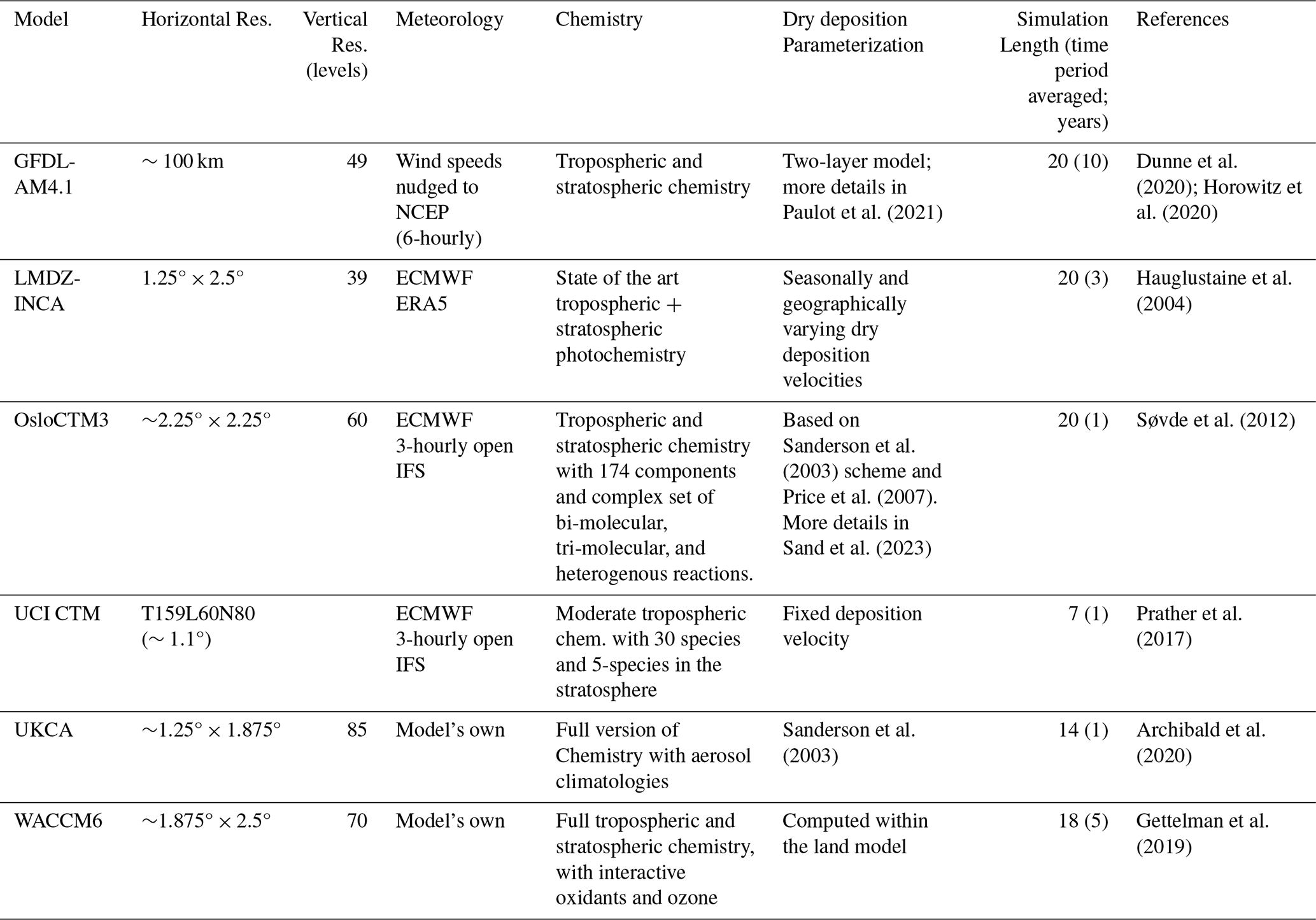
Here, we use the control simulations presented in Sand et al. (2023) for five models – OsloCTM3, UCI CTM, UKCA, LMDZ-INCA and GFDL-AM4.1. For WACCM6, we use a more recent simulation that is set up as the CTRL simulation described in Sand et al. (2023), except that it is run using CESM v. 2.1.2 and with 70 vertical levels (instead of 88 in Sand et al., 2023). All simulations use present-day (2010) atmospheric compositions and fixed hydrogen and methane surface concentrations. Further details on the models are provided in Table 1 and Sand et al. (2023).

Table 1 Details of the six models used here and Sand et al. (2023).

To evaluate model chemistry, we compare selected species that are critical to atmospheric production and loss of H₂, namely monthly model output for HCHO, OH, CO, NO₂ and NO. A qualitative comparison for these species is also made between the model results and satellite retrievals. Monthly-averaged satellite data for 2010 are downloaded for TROPOMI (Veefkind et al., 2012) for the time period between July 2018–June 2019 – to compare against the model simulations for the year 2010. The TROPOMI satellite has global daily coverage and retrieves multiple atmospheric trace gas components O₃, NO₂, and HCHO with a spatial resolution of 5.5 km × 3.5 km and an equator crossing time at about 13:30 local time. Column-averaged tropospheric values are post-processed to calculate annual averaged values for HCHO, NO₂, and CO (no averaging kernels are applied to the retrievals; vertical profiles are shown in Figs. A6, A7). Similarly, MOPITT data for CO (Deeter et al., 2003) for 2018 are compared to model results. This analysis is limited by the mismatch that arises due to the comparison of the monthly mean model outputs with satellite retrievals taken at a specific overpass time. To test how much this discrepancy can affect our comparison, we run an additional OsloCTM3 simulation for a year where the three hourly outputs are used.

2.2 Description of the isotope-coupled box model

Running the 3-D ACM takes substantial computing resources, limiting its applicability in evaluating the relationship between the different budget terms and the atmospheric concentration of hydrogen. We use a box model that calculates the change in global atmospheric H₂ based on production and loss at every timestep (one month; Eq. 1)

$$\begin{array}{}\text{(1)}& {\displaystyle \frac{\mathrm{d}C}{\mathrm{d}t}}=\mathrm{Production}-\mathrm{Loss}={\displaystyle \frac{E+P_{\mathrm{atm}}}{\mathit{\beta }}}-C{\displaystyle \frac{\mathrm{1}}{\mathit{\tau }}}\end{array}$$

where C is concentration in ppb; $\frac{\mathrm{d}C}{\mathrm{d}t}$ is change in concentration at every timestep; E corresponds to Emissions; P_atm is the atmospheric production of H₂; β is a factor used to convert from Tg to ppb; and $\frac{\mathrm{1}}{\mathit{\tau }}$ represents the loss terms as a lifetime calculated by $\frac{\mathrm{1}}{\mathit{\tau }}=\frac{\mathrm{1}}{{\mathit{\tau }}_{\mathrm{OH}}}+\frac{\mathrm{1}}{{\mathit{\tau }}_{\mathrm{Soil}}}$ where τ_OH and τ_Soil represent the lifetimes due to the OH radical and the soil-sink, respectively.

Emissions include time-varying emissions of H₂ from anthropogenic sources and biomass burning, and a constant natural source. Atmospheric production is calculated using time-varying methane concentrations and emissions of anthropogenic VOCs (including constant natural emissions). The two loss terms for atmospheric H₂ are represented by the soil-sink lifetime and the atmospheric lifetime.

A key aspect of this simple model is its flexibility, i.e. the model can be adapted to each atmospheric chemistry model. Atmospheric production, β-value (used to convert mass-values to concentration), and the loss terms vary between the 3-D models and are tied to one another. The anthropogenic and biomass burning emissions for H₂ are adapted for each model. The sinks are determined by setting the atmospheric and soil uptake lifetimes.

We include a function in the box model to calculate the isotopic composition of atmospheric H₂. The different sources and sinks of hydrogen have distinct isotopic signatures. Combining the burden and the isotopic values, we use a mass-balance approach to calculate the isotopic values of tropospheric H₂ at every time step. This is compared with modern-day observation and acts as a two-pronged check on the total budget. Unless otherwise stated, we use isotopic compositions for sources and sinks from Price et al. (2007) which are as follows: Anthropogenic emissions: −196 ‰; biomass burning: −290 ‰; atmospheric production (from CH₄ and NMVOCs): 162 ‰; Nitrogen fixation: −628 ‰ (Table 2). Fractionation factors of 0.943 and 0.58 are used for the soil-sink and OH loss, respectively. The box model does not account for the tropospheric-stratospheric H₂-cycling and the resulting tropospheric H₂-enrichment (Price et al., 2007; Pieterse et al., 2011). The stratospheric-tropospheric H₂ flux is not diagnostic output in the models considered in this study and this omission can result in a 29 ‰–37 ‰ offset in δD (Price et al., 2007; Pieterse et al., 2011, 2013).

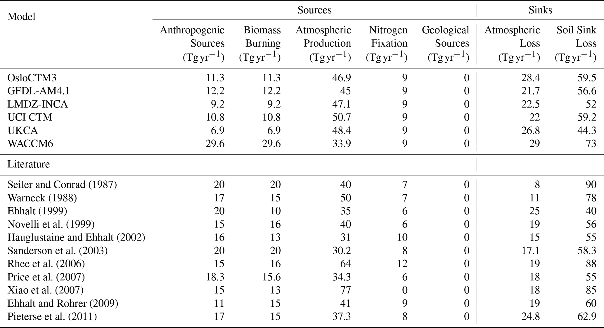
Table 2 Budget terms from the different ACMs in Sand et al. (2023) and published literature used in the box model study.

3 Results

The results section is organized as follows: first, atmospheric production and loss of H₂ are assessed in the six models by comparing key species involved in these reactions and evaluating them against satellite retrievals. Next, the temporal evolution of H₂ concentrations from the pre-industrial to today is evaluated using the box model. Two specific cases related to atmospheric production and loss are analyzed. Isotopic compositions are calculated in the box model to evaluate the overall tropospheric H₂ budget. Five scenarios are explored to demonstrate how a dual constraint based on concentration and isotopic composition can help constrain the various sources and sinks. An uncertainty analysis is also conducted by running the box model with 100 000 different combinations of sources and sinks picked using the Monte-Carlo approach to constrain their plausible ranges.

3.1 Atmospheric Production

Table 2 shows the different budget terms from the ACMs and previous literature studies. Atmospheric production values for the ACMs range from 34 Tg yr⁻¹ (WACCM6) to 56 Tg yr⁻¹ (OsloCTM3) for the models. The lower model values overlap the lower limit of the 38.4 ± 6.1 Tg yr⁻¹ estimate from Ouyang et al. (2025), with the higher model values exceeding it. The model spread is smaller than the range reported in published studies. Since the photolysis of HCHO is an important source of H₂, correctly capturing the background HCHO concentration is essential for constraining atmospheric H₂ production.

All models show broadly similar annual mean HCHO spatial patterns, with some regional differences (Fig. 1). GFDL-AM4.1, LMDZ-INCA, and UCI have higher HCHO concentrations over South America, Africa, and parts of East Asia. OsloCTM3 and UKCA exhibit lower concentrations over land, but higher over the oceans (Fig. A1). WACCM6 produces lower HCHO concentrations over land compared to the other models.

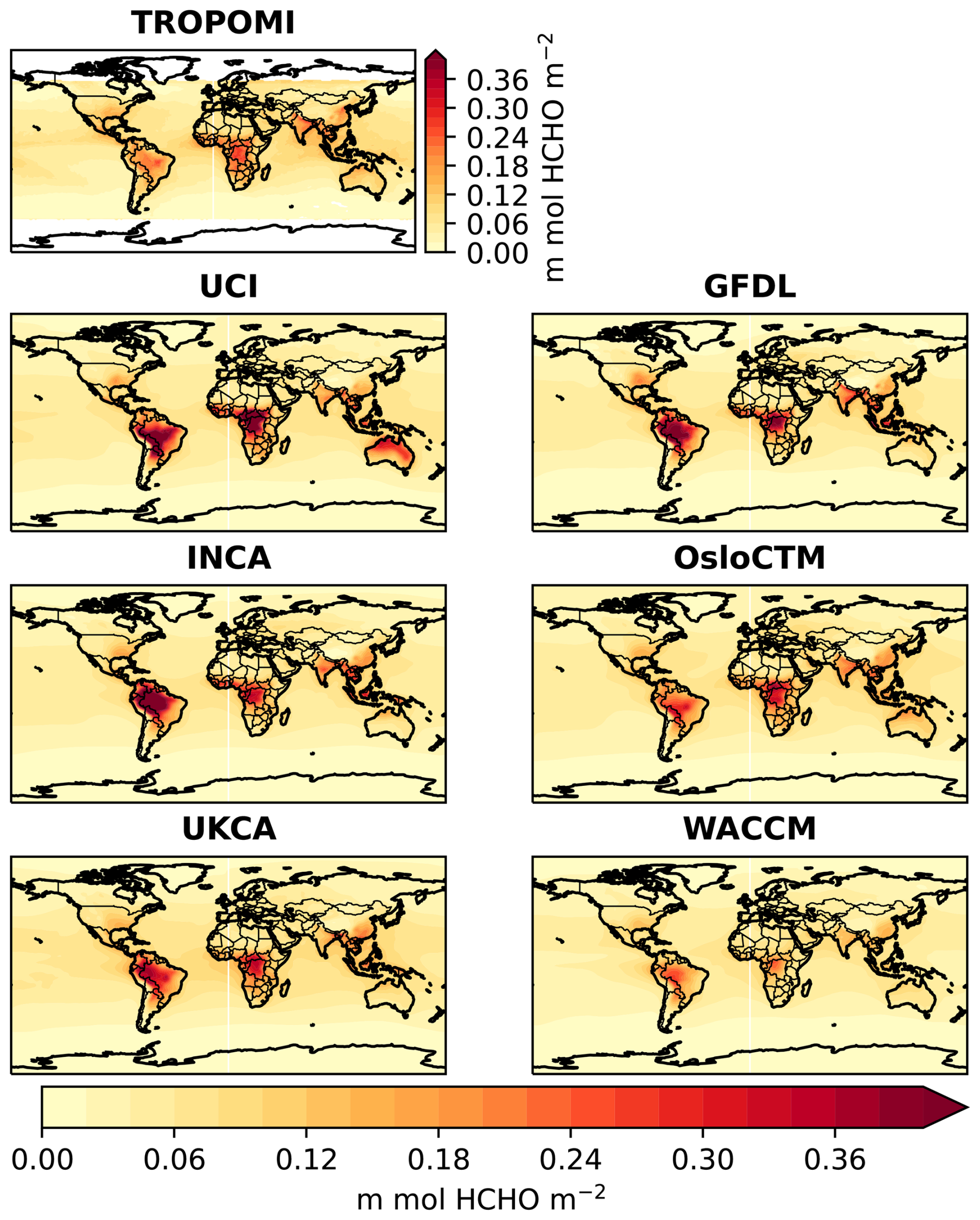
Figure 1 Spatial comparison of formaldehyde between TROPOMI satellite retrievals for July 2018–June 2019 and the different Atmospheric Chemistry Models listed in Table 1.

When compared with TROPOMI satellite retrievals, all models except WACCM6 produce reasonable HCHO concentrations, within 6.5 % of the TROPOMI retrieval; Figs. 1, A1). The multi-model mean for HCHO matches well with the TROPOMI global mean, albeit affected by the lower values from WACCM6. Broadly similar values between HCHO in the models and TROPOMI retrievals suggest that the 3-D models represent the production of atmospheric H₂ fairly well, however there are several uncertainties that can affect model simulations that have not been explored in this study, such as the uncertainty in the photodissociation of HCHO, and biogenic NMVOC emissions. Furthermore, all models show a large bias in the Southern Ocean compared to the TROPOMI retrieval (Fig. A4). Reasons for these differences between the models and the satellite retrievals will be explored in future work.

Additionally, we also compared model results against ATom measurement campaigns for nine different regions and four seasons (Figs. A6–A7). All models have comparably similar vertical profiles. They generally also match the ATom measurements other than in the West Atlantic (A3) in the summer and autumn; and North Pacific (P1) in the summer, and winter.

3.2 Atmospheric Loss

Atmospheric loss in the ACMs ranges from 21 Tg yr⁻¹ (GFDL-AM4.1) to 28 Tg yr⁻¹ (OsloCTM3). This spread is larger than 18.4±2.2 Tg yr⁻¹ for 2010–2020 estimated in Ouyang et al. (2025) and other published studies (Table 2). The atmospheric loss of H₂ is primarily driven by its reaction with OH, a key oxidant in the atmosphere. Due to the short lifetime of OH (<1 s), direct retrievals of OH concentrations are not possible, therefore limiting a model-data comparison for OH. Indirect approaches, such as the use of a combination of CO and NO_x concentrations have been used to estimate OH levels for urban plumes and specific emission sources (Dalsøren et al., 2016; Lama et al., 2022). Although OH chemistry is influenced by several factors – such as photolysis reactions, temperature, tropospheric ozone, humidity, methane and NMVOCs – NO_x generally acts to increase OH concentrations and CO reduce the OH concentrations.

In Fig. A2, we show model outputs for CO, OH, and NO₂ along with satellite retrievals for CO from TROPOMI and MOPITT, and NO₂ from TROPOMI. All models show broadly similar spatial patterns albeit with some regional differences in magnitude. Compared with satellite retrieval, all models simulate larger values for NO₂, with the global means at least twice that of retrievals (Fig. A4). These differences are seen both over land and oceans (Figs. A2a and A4). This overestimation may result from comparing monthly mean outputs with satellite retrievals, which are restricted to specific overpass times and air mass factors. As the simulation and the satellite reanalysis datasets are for two different time-periods, we cannot replicate the specific air mass factors in OsloCTM3, limiting this comparison. But if we restricted mean calculations to specific satellite overpass times with the 3-hourly OsloCTM3 simulation, OsloCTM3 results show much lower values, bringing the model means closer to TROPOMI values, with an underestimation (Fig. A4a). The effect of using the ratio of NO₂ during overpass to the monthly mean for OsloCTM3 for the other models is shown in Fig. A8 where there is a decrease in model NO₂ for all models, more in line with the satellite retrieval. Thus, comparing the monthly mean model output with satellite-overpass times only allows for a broad qualitative analysis. Future simulations should save the 3-hourly output so that such comparisons can be made.

For CO, the models are broadly consistent with one other, with a multi-model standard deviation of 0.002 mol CO m⁻². The inter-model spread is larger over land (0.003 mol CO m⁻²) than over oceans (0.001 mol CO m⁻²). These results can be compared against TROPOMI and MOPPITT, which are broadly consistent with each other (Fig. A2b), with a global mean difference of 0.002 mol CO m⁻². Over the oceans, the difference between the two satellite retrievals is 0.003 mol CO m⁻², while over land it is 0.001 mol CO m⁻². All models underestimate CO relative to the satellite retrievals, with large differences (10 %–20 %) over the Northern Hemisphere mid- and high latitudes. WACCM6 and OsloCTM3 have lower CO values compared to GFDL-AM4.1 and LMDZ-INCA models. Although the global mean differences between MOPITT and TROPOMI are similar to the multi-model standard deviation, the models have lower CO over land, compared to the satellite retrievals. All models also do a reasonable job of matching the vertical profiles of CO observed during the ATom campaign (Figs. A1 and A2). GFDL-AM4.1 and INCA have lower ${\mathrm{NO}}_{\mathrm{2}}/\mathrm{CO}$ ratio values compared to OsloCTM3, consistent with the elevated OH concentration in OsloCTM3 (Fig. A2c, d). Our results suggest that OH differences between models could be related to the local chemical environment (${\mathrm{NO}}_{\mathit{\text{x}}}/\mathrm{CO}$ differences) with models showing a larger ${\mathrm{NO}}_{\mathrm{2}}/\mathrm{CO}$ ratio having larger OH values or vice versa. This could explain some of the diversity in atmospheric loss of H₂ in the models.

3.3 Box Model

Here, we use the box model for two applications: (1) to model the sensitivity of modelled H₂ concentrations from pre-industrial to 2015, to two input parameters that impact atmospheric production and loss, and (2) evaluate the feasibility of the different sources and sinks using isotopic values.

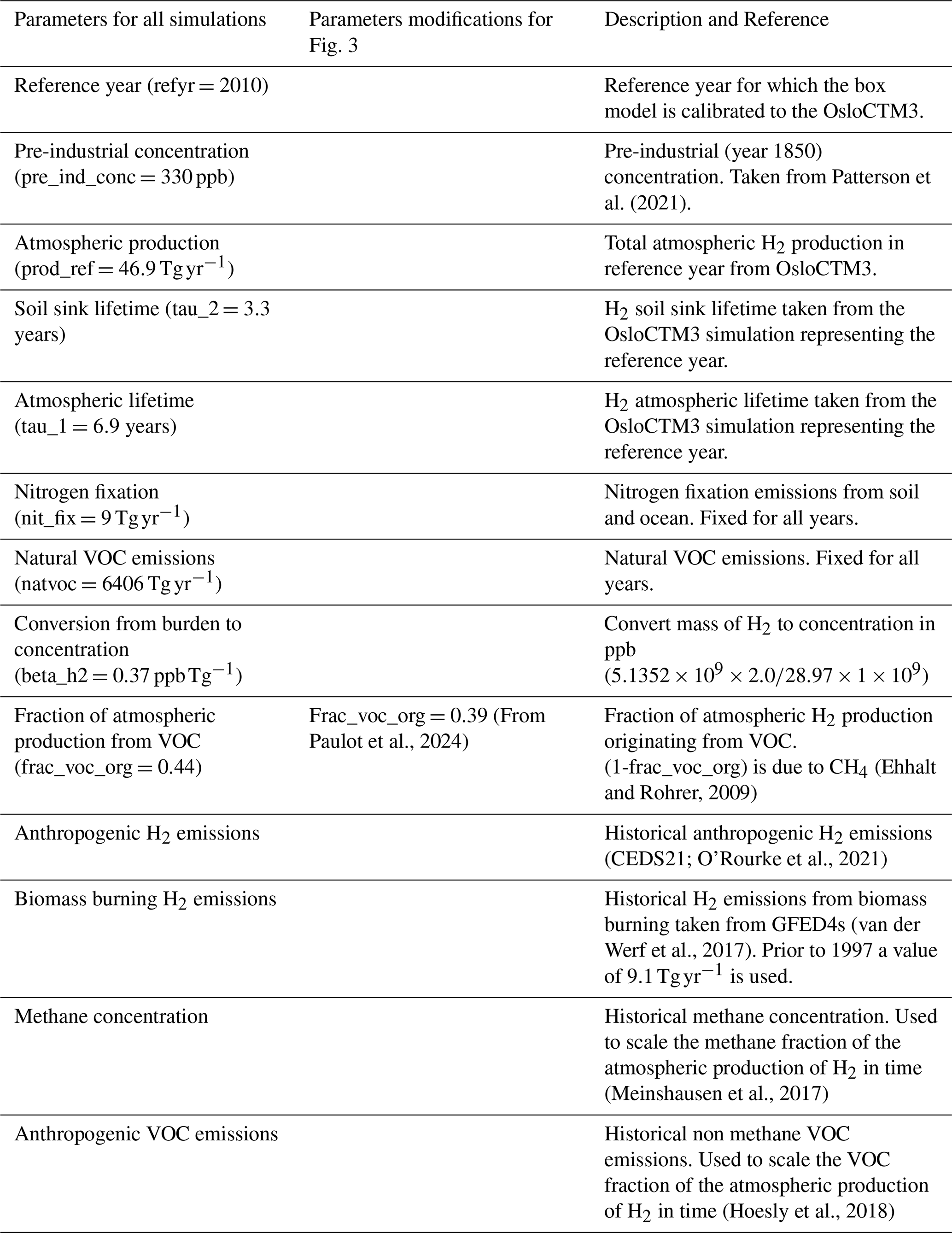
Although 3-D model simulations have been conducted for the modern-day time slices, simulating the temporal evolution of tropospheric H₂ from the pre-industrial period to 2015 using 3-D models is computationally very intensive and often prohibitive, making box models an attractive alternative (Fig. 2). The box model is initialized using an inferred pre-industrial H₂ concentration of 330 ppb (Patterson et al., 2020, 2021) and model parameters are chosen based on existing datasets (Table A1). While these choices are not unique, the goal here is to present the model sensitivity to two specific parameter choices – split of atmospheric H₂ production between CH₄ and VOCs, and the atmospheric H₂ loss mediated by the lifetime of OH. All parameters are adjusted so that they match the model results for the present-day OsloCTM3 simulations panel (a) shows the evolution of the different emission and production terms of the budget in the box model, with anthropogenic emissions of H₂ scaled to CO emissions and atmospheric production following CH₄ concentrations showing a rise after the 1970s. Atmospheric H₂ production from NMVOCs also increases slowly post-1970s from ∼20 to ∼25 Tg yr⁻¹. Nitrogen fixation is set constant at 8 Tg yr⁻¹ through the simulation and biomass burning emissions are set at 8 Tg yr⁻¹ till the 1990s, following which emissions are allowed to vary. Figure 2b shows the split between total emissions and atmospheric production and Fig. 2c shows the resulting evolution of global mean tropospheric concentration of H₂. Crosses in Fig. 2b and c indicate H₂ concentrations from pre-industrial and present-day OsloCTM3 simulations.

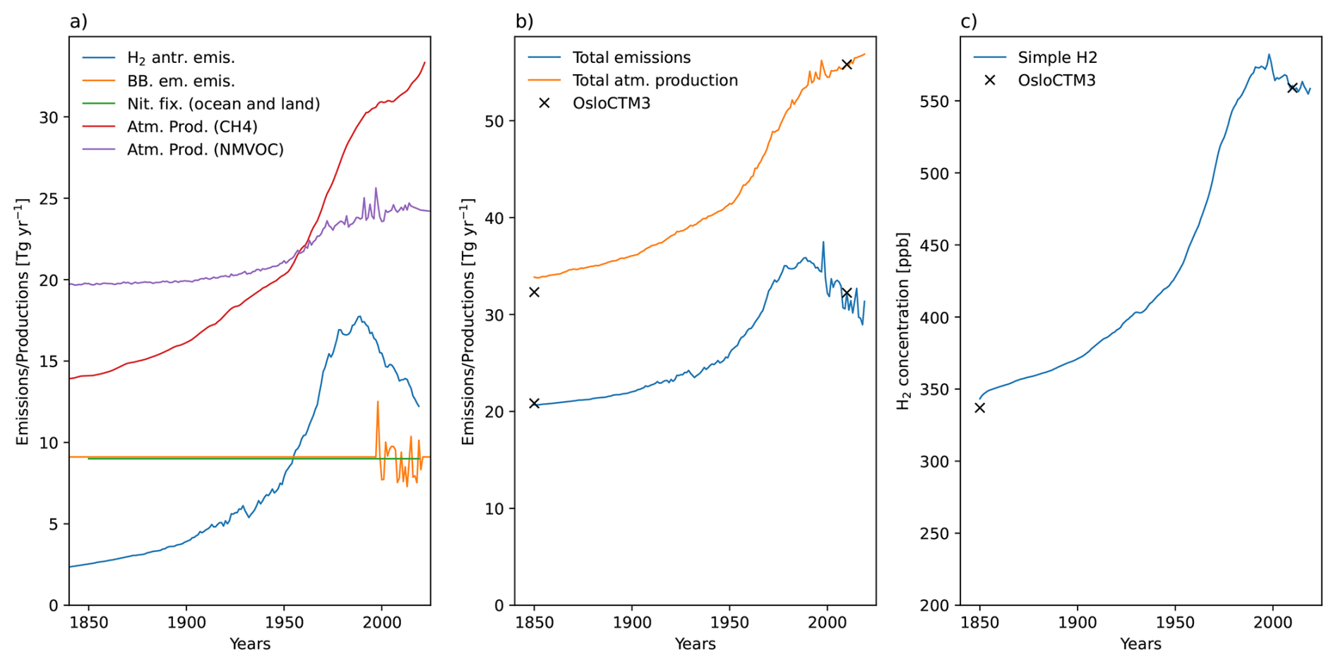
Figure 2 Temporal evolution from 1850 to 2015 of (a) emissions and atmospheric production; (b) total atmospheric production and total emissions; and (c) atmospheric concentration of H₂ from pre-industrial to today from the box model fitted to the OsloCTM3 model. The crosses indicate the pre-industrial (1850) and the modern day (2010) results from the OsloCTM3.

While the box model allows exploration of various uncertainties in H₂ evolution, such as the impacts of natural vs. anthropogenic emissions, different emission inventories, and the use of variable versus fixed soil-sinks - this study focuses on two specific issues related to atmospheric production and losses. A key question regarding atmospheric production is the significance of the relative contributions of H₂ production from CH₄ or NMVOCs. Total production is the sum of production from CH₄ and NMVOCs (not diagnosed in the ACMs), with the increase in production from CH₄ showing a larger increase over time. The box model can be used to test the impacts of modifying this split (Fig. 3). We run two cases – in the first case (solid lines in Fig. 3), production from NMVOCs accounts for 44 % of the total production consistent with the estimate of Ehhalt and Rohrer (2009), while in the second case (dashed lines in Fig. 3), this production from NMVOCs is reduced to 39 % following Paulot et al. (2024). For the first case, the crossover when production from CH₄ surpasses production by NMVOCs occurs in the 1950s (solid pink and blue lines in Fig. 3a), while in the second case, this crossover occurs in the 1910s (dashed pink and blue lines in Fig. 3a). In the first case, the pre-industrial H₂ production from NMVOCs decreases from ∼20 to ∼13 Tg yr⁻¹, while production from CH₄ increases from ∼14 to ∼18 Tg yr⁻¹ (Fig. 3a). Total production in 1850 is reduced by ∼4 Tg yr⁻¹ with the gap narrowing over time until the 1980s, when both cases converge. The maximum difference in H₂ concentration between the two cases does not exceed ∼15 ppb.

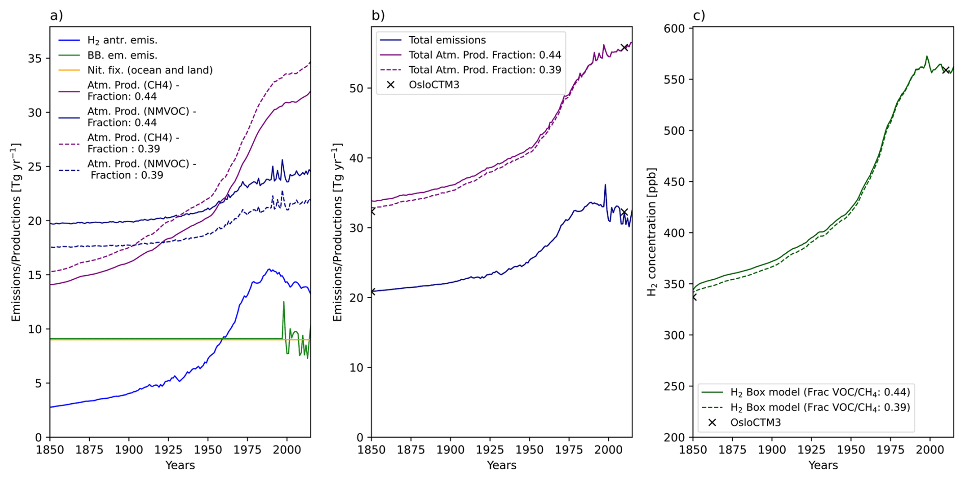
Figure 3 Similar to Fig. 2, but with different relative contributions of atmospheric production via CH₄ and VOCs. Solid lines represent values from a box model simulation with a $\mathrm{VOC}/{\mathrm{CH}}_{\mathrm{4}}$ production ratio of 0.44 from Ehhalt and Rohrer (2009), while stippled lines indicate results from a box model simulations with the ratio of 0.39 from Paulot et al. (2024).

In the box model, atmospheric losses are defined by their lifetime, which depend on OH concentrations. We assess the effect of different temporal evolution of lifetimes due to OH concentrations on tropospheric H₂, by running the model with three different atmospheric lifetimes that correspond to: (1) constant OH concentrations from pre-industrial to today; (2) pre-calculated OH concentrations by combining historical trends from Stevenson et al. (2020) and Skeie et al. (2023a); and (3) using a scheme from the Third Assessment Report (TAR) where the OH-sink lifetime is adjusted following Ehhalt et al. (2001; Table 4.11, footnote b) based on CH₄ concentrations, and emissions of CO, NO_x, and VOCs (Fig. 4). The impact of the different OH concentrations on the OH-sink lifetime is shown in Fig. A11. Note that the OH concentrations here only affect the losses/sink term and not atmospheric production. These results indicate that using constant versus pre-determined OH-sink lifetimes produce similar H₂ concentrations (within 10 ppb) through time. In contrast, applying the TAR scheme leads to higher H₂ concentrations, ∼40 ppb greater than the other cases until the early 1970s – a couple of decades after the increase in anthropogenic emissions and a few years after the crossover point when atmospheric production from CH₄ dominates over production from NMVOCs. This indicates a higher atmospheric lifetime early in the box model simulation (pre-1940s) as calculated by CH₄ concentrations, and emissions of CO, NO_x, and VOCs. Notably, all these terms have a large uncertainties. After the 1970s, the H₂ concentration from the three atmospheric lifetime cases broadly match each other.

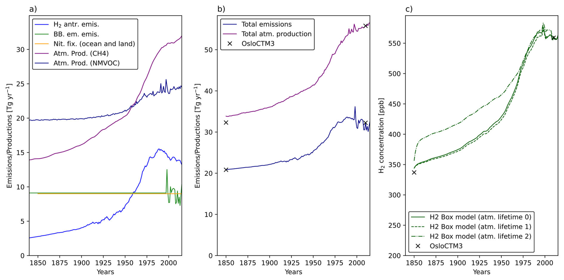
Figure 4 Similar to Fig. 3, but (c) shows the impact of having different atmospheric lifetimes due to different OH concentrations. The three OH-based lifetimes are calculated as Atm. Lifetime 0: Time-variant OH based on trends in Stevenson et al. (2020) and Skeie et al. (2023a); Atm. Lifetime 1: Constant OH leading to constant atmospheric lifetime; Atm. Lifetime 2: time-variant OH using equations from the Third Assessment Report (Ehhalt et al., 2001).

Results indicate that the various assumptions in the box model for the split between H₂ production from NMVOCs and CH₄ and for the time evolution of the atmospheric lifetime, which are not provided by the ACMs, have only a small effect on the H₂ concentration over recent decades.

3.4 Isotopic evaluations using the Box Model

In addition to H₂ concentrations, isotopic values of atmospheric H₂ are calculated in the box model at every time step, depending on the relative contributions from the different sources and sinks. Figure 5 shows the hydrogen atmospheric concentration vs. isotopic composition for the different box model simulations fit to match the ACMs (using model parameters as inputs for steady-state 2010 conditions) and from published literature. All the models' box model simulation results show a narrow range of atmospheric H₂ concentrations (520–540 ppb; by design) and a wider range for isotopic values (20 ‰–210 ‰), with WACCM6 at the lower-end and UKCA at the higher-end. The enriched isotopic value in WACCM6 is due to the combination of high emissions (anthropogenic and biomass burning sources), low atmospheric H₂ production and high soil sink. The more negative value for isotopic composition in UKCA is due to low emissions and low soil sink in UKCA. OsloCTM3 has higher atmospheric production, but this is isotopically balanced out by higher soil sink. Published studies have ranges for both predicted H₂ and isotopic values of 365–550 ppb and 0 ‰–150 ‰ respectively. That the isotopic range is large is not surprising as most of these studies look at the concentration budget and not the isotopic budget. For example, Fig. A9 shows the resulting budgets if isotopic values and fractionation factors for the different sources and sinks are taken from Pieterse et al. (2011) rather than Price et al. (2007) without and with stratospheric enrichment of 29 ‰. The mean changes for the models and literature values are 7.8 ‰ and 24.56 ‰ without stratospheric enrichment and 20.61 ‰ and 49.61 ‰ with the stratospheric enrichment respectively. This difference is driven by the Pieterse et al. (2011) having isotopic compositions of −260 ‰ and 116 ‰ for biomass burning and atmospheric production of CH₄ instead of −290 ‰ and 162 ‰ in Price et al. (2007). We present this spread here, not to evaluate them against models, but to reiterate the benefit of combining H₂ concentrations with δD to constrain the different budget terms.

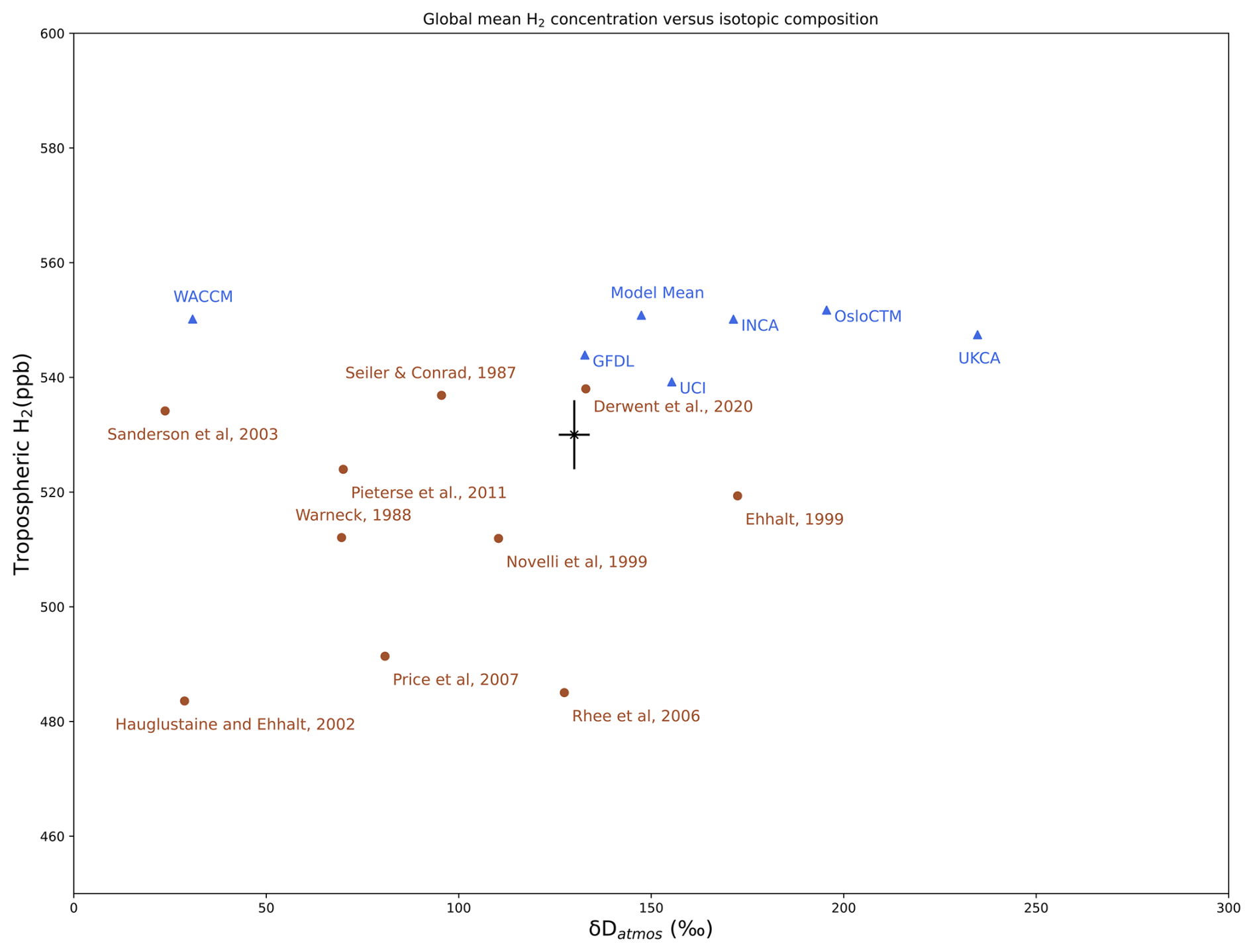
Figure 5 Relationship between atmospheric hydrogen mole fraction and isotopic composition (δD) from different models (triangles) and published literature (circles). The cross indicates the observed range of lower tropospheric H₂ concentrations between 1991–1996 of 531±6 ppb (Novelli et al., 1999) and δD values (Price et al., 2007; the sensitivity to using values from Pieterse et al. (2011), is shown in Fig. A9). The model concentrations are higher than observed because they are calibrated for more recent observations.

We present five cases where the sources and sinks are modified to demonstrate this approach (Fig. 6): (1) a base case using modern-day values; (2) high atmospheric production where atmospheric production values from a top-down estimate (Rhee et al., 2006) are used; (3) low atmospheric production; (4) additional geological source of 23 Tg yr⁻¹ as suggested by Zgonnik (2020) and (5) the additional geological source of 23 Tg yr⁻¹ along with a high OH sink. To balance the budget for H₂-concentrations, we adjusted the soil sink (Table 3). These cases are chosen to constrain the range of atmospheric production estimates and potential geological inputs by evaluating the feasibility to fall within observed concentration and isotopic ranges. It should be noted that geological sources can span a wide range of isotopic values from 0 ‰ to −1000 ‰. We choose a value of −385 ‰ which is the mean of the white hydrogen values suggested in Gibson et al. (2024). The effect of using a different isotopic value for a geological source is shown in Fig. A10.

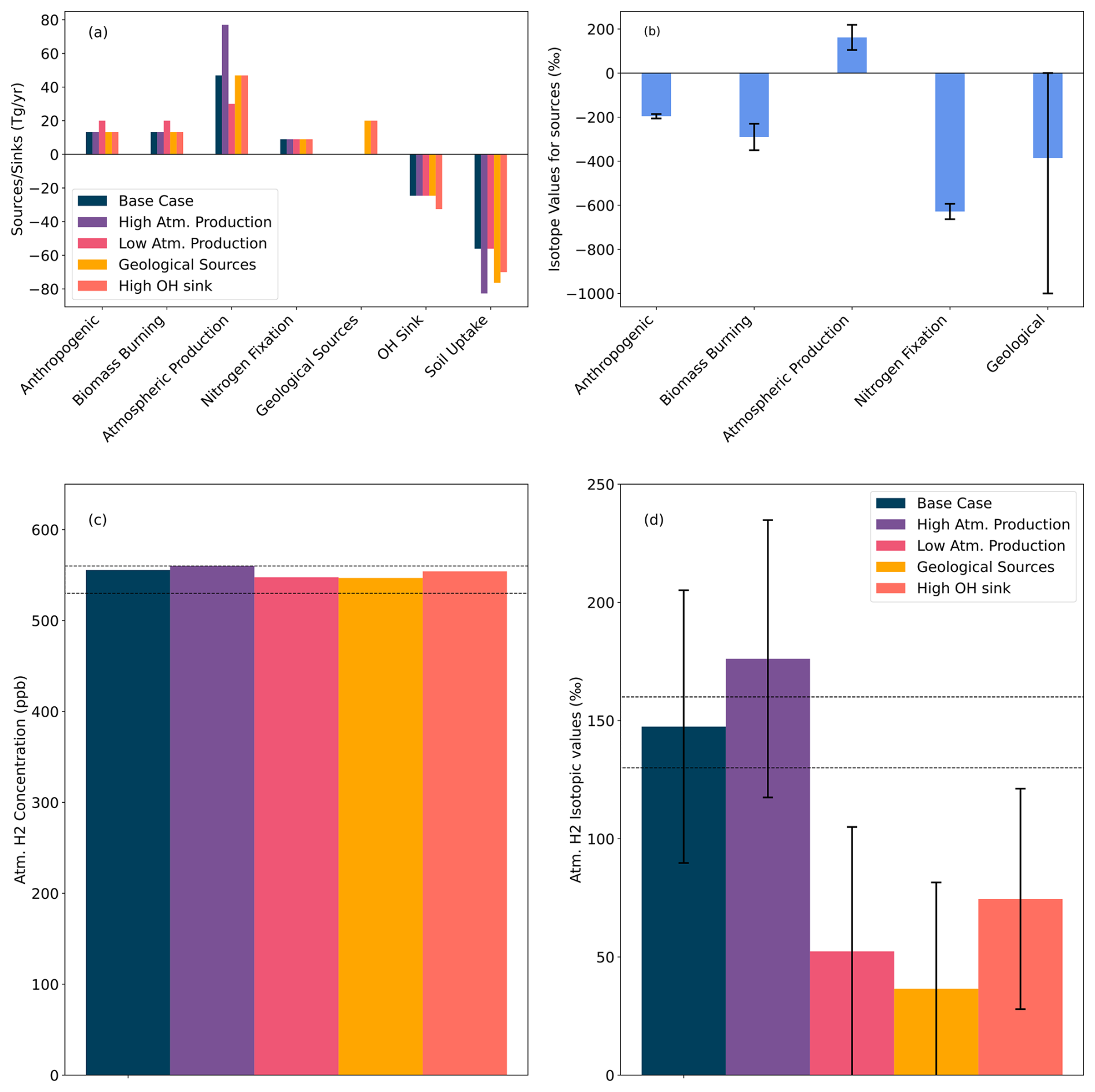
Figure 6 Box model results with isotopic calculations for the Base case (dark blue bars), high atmospheric production (purple), low atmo-spheric production (pink) and geological sources (yellow) (a) showing the different sources and sinks used in the box model; (b) isotopic values for the sources used in box model; (c) calculated H₂ concentration; and (d) calculated isotopic values for tropospheric H₂ for the different cases. The dashed black lines show the observed ranges with H₂ concentration taken here as 530–560 ppb and H₂ isotopic compositions as 130 ‰ to 160 ‰.

Table 3 Values used for the emissions, isotopic values for the sources and lifetime and fractionation factors used for the four different cases in the box model with steady-state 2010 conditions.

Figure 6a shows the magnitude of the different sources and sinks for hydrogen in the five cases and Fig. 6b shows the isotopic values for the sources used in the box model. The resulting hydrogen concentrations for the four cases are shown in Fig. 6c. By design all five cases produce atmospheric concentrations that are broadly near the observed concentration range (530–560 ppb, dashed lines). However, the corresponding isotopic compositions are much more sensitive compared to H₂ concentration and fall far outside the observed ranges (130 ‰–160 ‰) for the three perturbed cases. This clearly indicates that low and high atmospheric production values do not agree with the observed H₂-isotopic values. Further, a geological source (with a corresponding increase in soil uptake) shows an even bigger shift in δD – not observed today.

Uncertainty ranges for the isotopic signatures of each source were used to calculate the maximum possible uncertainty. The most depleted and enriched source combinations were applied to calculate the minimum and maximum ranges shown in Fig. 6d. These results indicate that while high atmospheric production can be accommodated within the budget if extremely depleted isotopic values are used for the other sources, scenarios with lower atmospheric production and high geological sources do not fit the budget.

We also performed an uncertainty analysis to evaluate the joint uncertainties using the distributions of all the sources and sinks and their isotopic values (ranging from the most negative and most positive values in literature; Fig. 7). Additionally, we also check the impact of the stratospheric contribution to the analysis, by assuming the enrichment of the final atmospheric δD composition by randomly picking a value between 29 ‰–37 ‰. We use a Monte-Carlo approach by randomly picking 100 000 different combinations of sources and sinks to run the box model and check whether the resulting atmospheric concentration and the isotopic composition of atmospheric H₂ is within the ranges of 530–560 ppb (to account for the increasing trend till 2021) and 130 ‰–160 ‰, respectively. Applying the joint certainly analysis, the 97.5th percentile upper bound on the geological sources decreases from 9.4 Tg yr⁻¹ in the initial distribution to 6.3 and 7.7 Tg yr⁻¹ without and with a stratospheric contribution, respectively. Relative to the initial distribution, only 88 % and 91 % of the geological flux distribution overlap with the 95 % constrained intervals without and with a stratospheric contribution, ruling out 12 % and 9 % of the distribution, respectively.

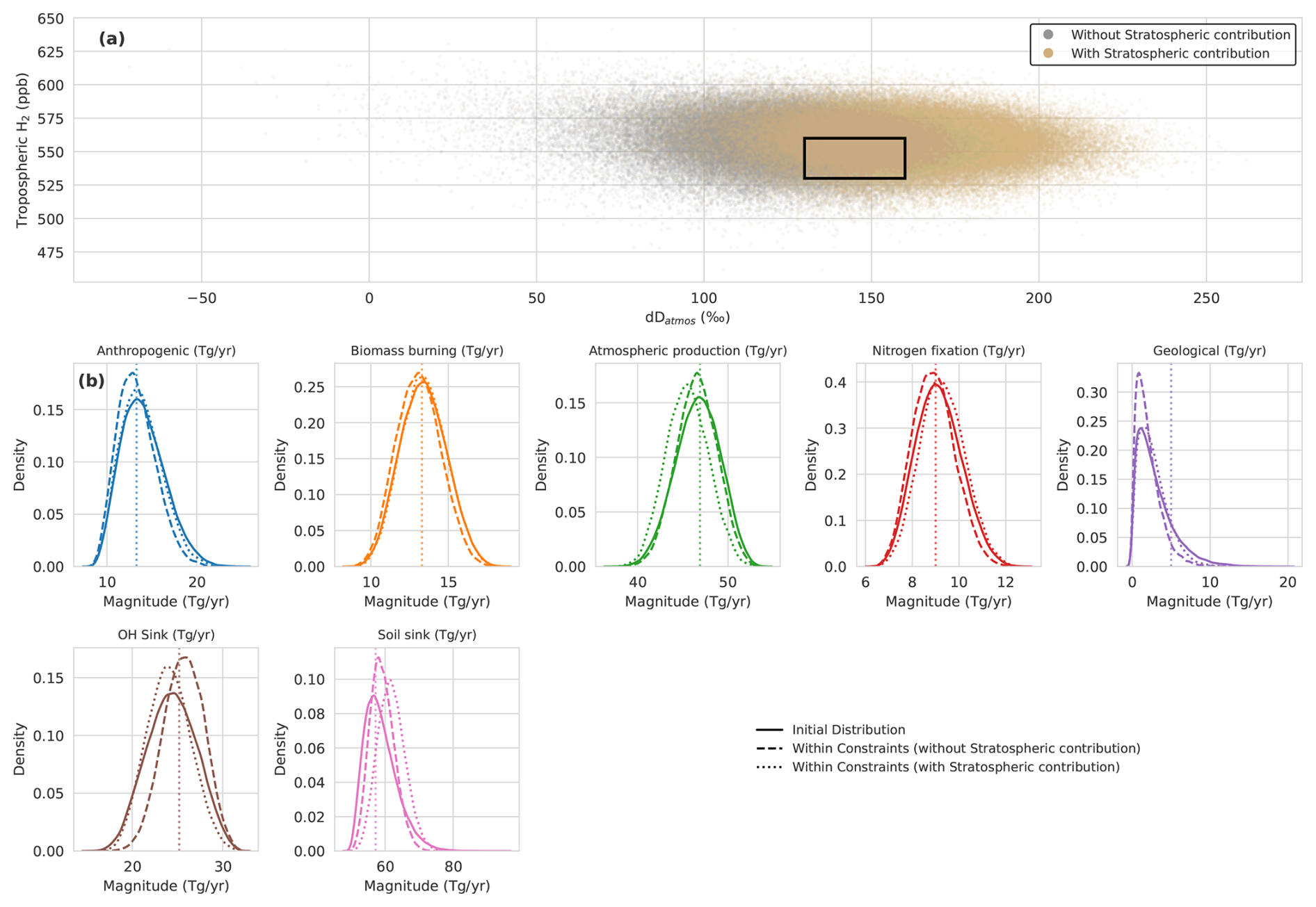
Figure 7 Joint analysis of the different sources and sinks and isotopic compositions and the resulting probably density function changes with and without stratospheric contribution. The distributions for the different sources and sinks are all beta-distributions within the ranges found in published literature and models, while for geological sources we used a log-normal distribution for the source term. The isotopic ranges are the minimum and maximum values found in literature. The box model is run 100 000 times with samples being randomly picked from the distributions. For the stratospheric contributions, a value between 29 ‰–37 ‰ is also randomly picked and added to calculate the final isotopic composition of the atmospheric H₂.

The influence of the individual sources and sinks on the final tropospheric mole fraction and isotopic composition of tropospheric H₂ is shown in Fig. 8 as the effect of a 2 % change in the source or sink strength. Among the sources, atmospheric production has the largest effect on both the tropospheric H₂ and isotopic compositions, with each of the other sources having less than 1/3rd of the impact. The two sinks also play a huge role with the soil sink making the isotopic values more negative, while the OH sink shifting them to more positive values.

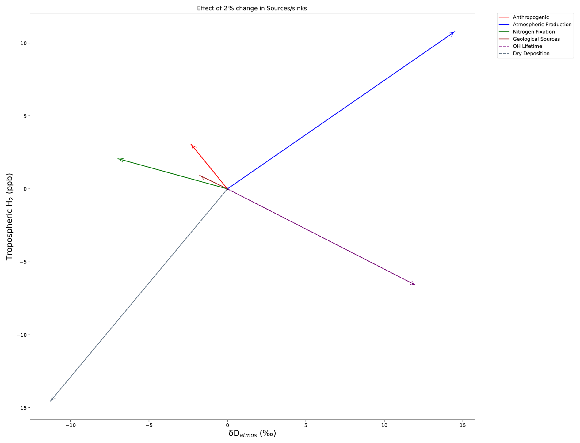
Figure 8 Impact of a 2 % change in individual sources and sinks on the tropospheric mole fraction and the isotopic composition of H₂.

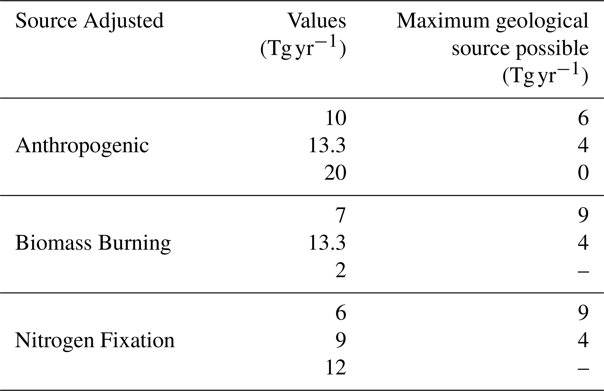
We extend this analysis by evaluating what adjustments to individual sources would be required to accommodate geological sources. While multiple source-sink combinations exist that fit within the concentration and isotopic constraints, we restrict this sensitivity analysis to emissions from anthropogenic sources, biomass burning, and nitrogen fixation. Based on model evaluations and box model constraints the atmospheric production and soil sink are allowed to vary between 37–60 and 49–77 Tg yr⁻¹ respectively. The range for soil sink is derived by running the box model across the specified range of atmospheric production values to identify feasible soil sink estimates that satisfy the observed concentration and isotopic constraints for tropospheric H₂.

Table 4 shows the maximum geological source consistent with low, mid, and high estimates of the three sources. The results indicate that the maximum plausible geological source given the constraints is 9 Tg yr⁻¹. Thus an estimate of 23 Tg yr⁻¹ as suggested by Zgonnik (2020) is not possible with our assumed isotopic composition of the geological input. However, greater contributions from isotopically enriched volcanic sources can affect this upper bound.

Table 4 Maximum allowable geological source input, constrained by adjusting emissions from anthropogenic, biomass burning, and nitrogen fixation within their respective observed low, mid, and high ranges.

4 Implications and conclusions

Chemical comparisons for atmospheric production and loss show that the models broadly match each other spatially for HCHO, NO₂, and CO. Ranges for the different sources and sinks for the models and from published literature are shown in Fig. 9. The ranges for atmospheric production and atmospheric loss budget terms from published literature range from 37–80 and 15–20 Tg yr⁻¹. A recently published global hydrogen budget for 2010–2020 suggests values of 38.4±6.1 and 18.4±2.2 Tg yr⁻¹ for photochemical production and sink, respectively. All model values are below the two highest estimates of atmospheric production using the top-down estimates. Isotopic evaluations using the box model also show that these high values of atmospheric production lie outside the range of observed isotopic ranges (Fig. 6). These suggest that atmospheric production values lie within the range of 37–60 Tg yr⁻¹ as shown in Fig. 9. Atmospheric loss in the models is higher than that documented in literature – possibly related to the range in OH concentrations in the models (Yang et al., 2025). However, lacking OH observations and to balance the budget, we suggest a larger range for atmospheric loss of 15–30 Tg yr⁻¹. Soil sink estimates are constrained to 49–77 Tg yr⁻¹, given the new constrained range in atmospheric production.

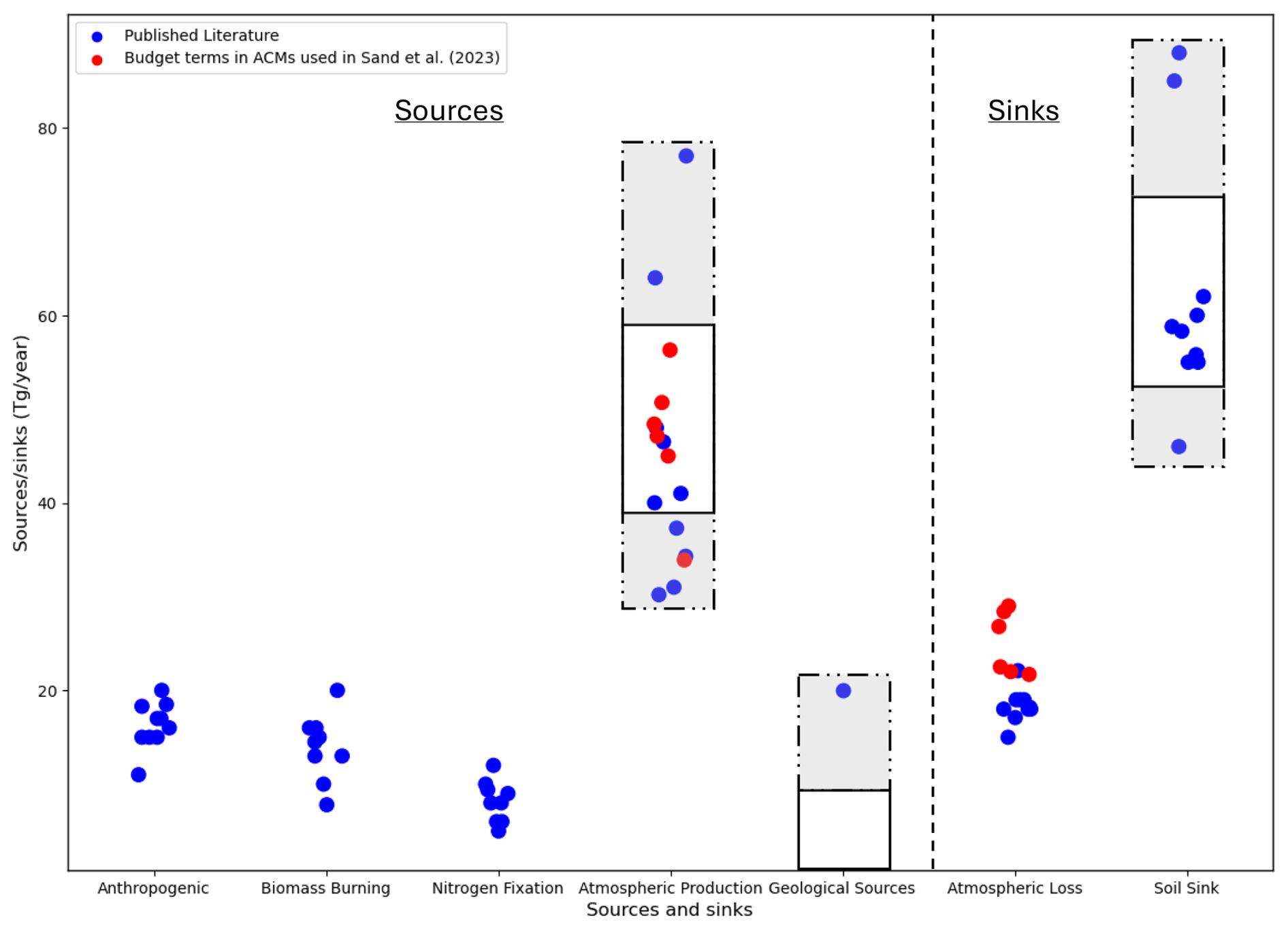
Figure 9 Sources and sinks in the tropospheric hydrogen budget, showing updated ranges for atmospheric production, atmospheric loss based on this study. The grey shaded area with dashed outlines represents previously reported ranges, while the solid white boxes indicate the updated ranges. Model values are shown for the atmospheric production and loss terms that are analyzed in this study.

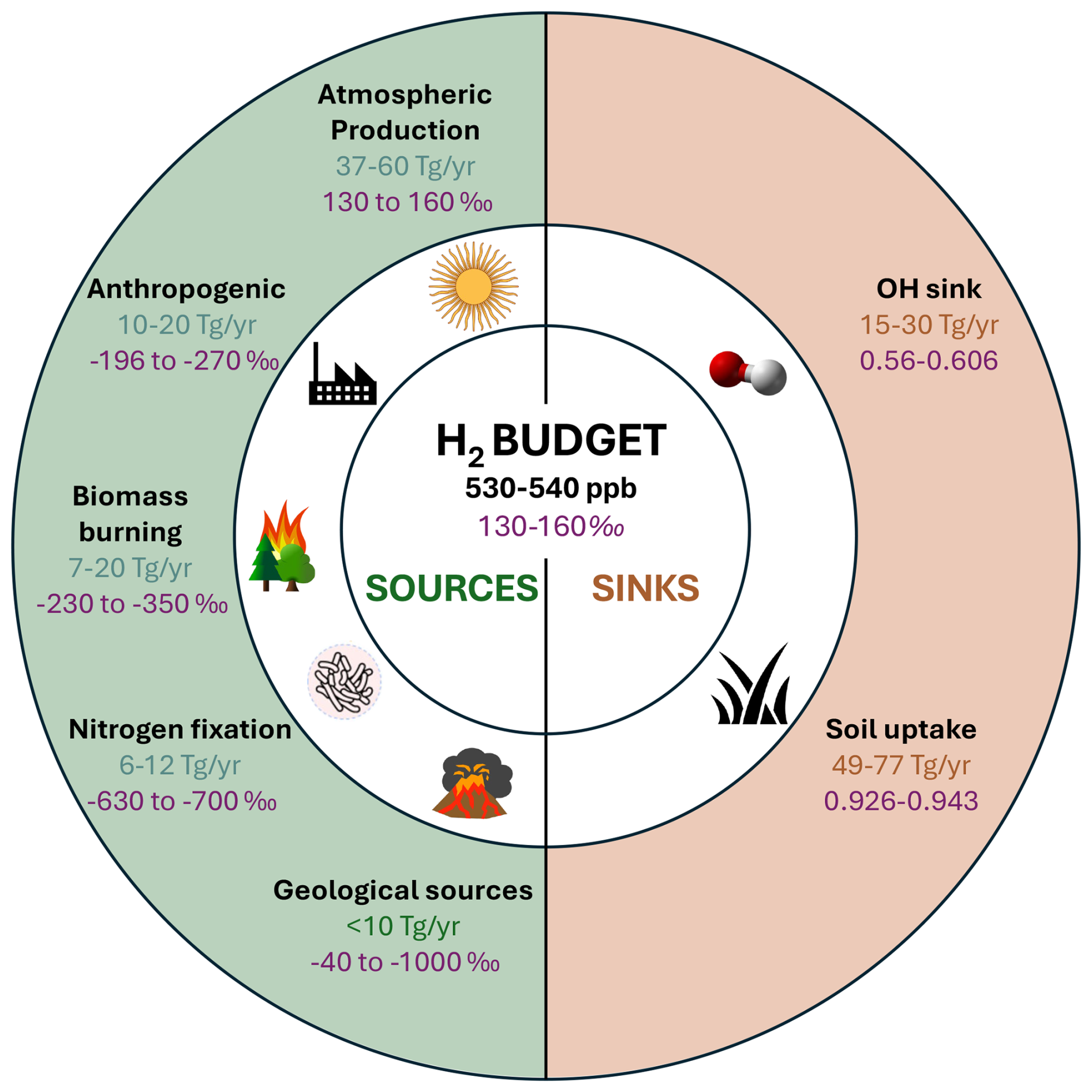
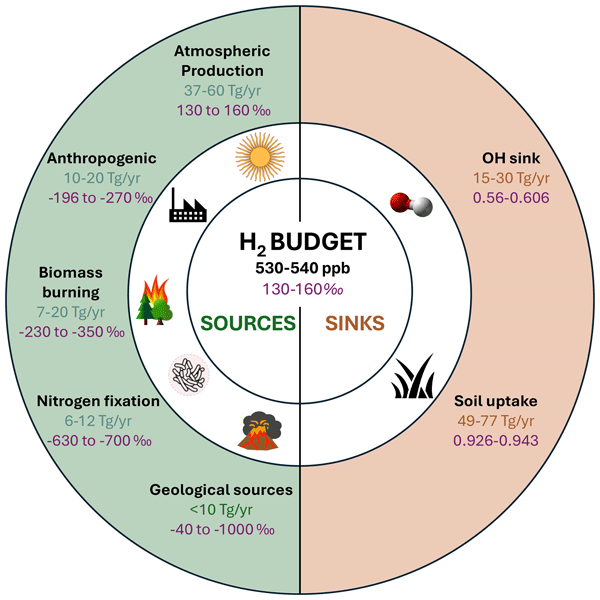
Figure 10 An updated estimate of source and sink ranges based on existing literature and this study. Numbers include the range of sources (green) and sinks (brown) in Tg yr⁻¹ and isotopic values of sources and fractionation factors for the sinks (in purple).

This study is limited by the uncertainties associated with each budget term (both concentrations and isotopic values), whether from observational estimates or models. Using geological sources with enriched isotopic values of −100 ‰ to 0 ‰, rather than −385 ‰ that we use, would allow for a larger geological input but it would still require a rearrangement of the other budget terms. Other potential validations of the budget, such as seasonal variations, recent trends and a more detailed analysis of the latitudinal variations of hydrogen are also beyond the scope of the current setup of the box model.

Our results show that six different ACMs with different chemistry schemes show similar HCHO tropospheric mole fraction – a proxy used here to evaluate atmospheric production and broadly match TROPOMI satellite retrievals. There is a larger diversity in OH indicating more uncertainty and a bigger spread for atmospheric losses. These could be related to different chemistry and different ${\mathrm{NO}}_{\mathit{\text{x}}}/\mathrm{CO}$ chemical environments in the models. We employ a box model to simulate the evolution of atmospheric H₂ from pre-industrial to today, exploring the impacts of having different ${\mathrm{CH}}_{\mathrm{4}}/\mathrm{VOC}$ relative contributions for atmospheric production and OH lifetimes for atmospheric losses. The ability of the box model to reproduce the broad trends in H₂-concentrations over time suggests that the budget terms reasonably represent the global H₂ cycle. Using combined constraints from atmospheric concentrations and isotopic values, the box model suggests atmospheric production to be in the range of 37–60 Tg yr⁻¹. Photochemical losses are constrained to 15–30 Tg yr⁻¹ and soil sink is constrained to 49–77 Tg yr⁻¹ (Fig. 10). These values are more consistent with the “bottom-up” estimates and reflect our current understanding based on a combination of model analysis, and expert judgment. Our study highlights the critical need for more isotopic observations of atmospheric H₂ to refine our understanding of the hydrogen budget.

Appendix A

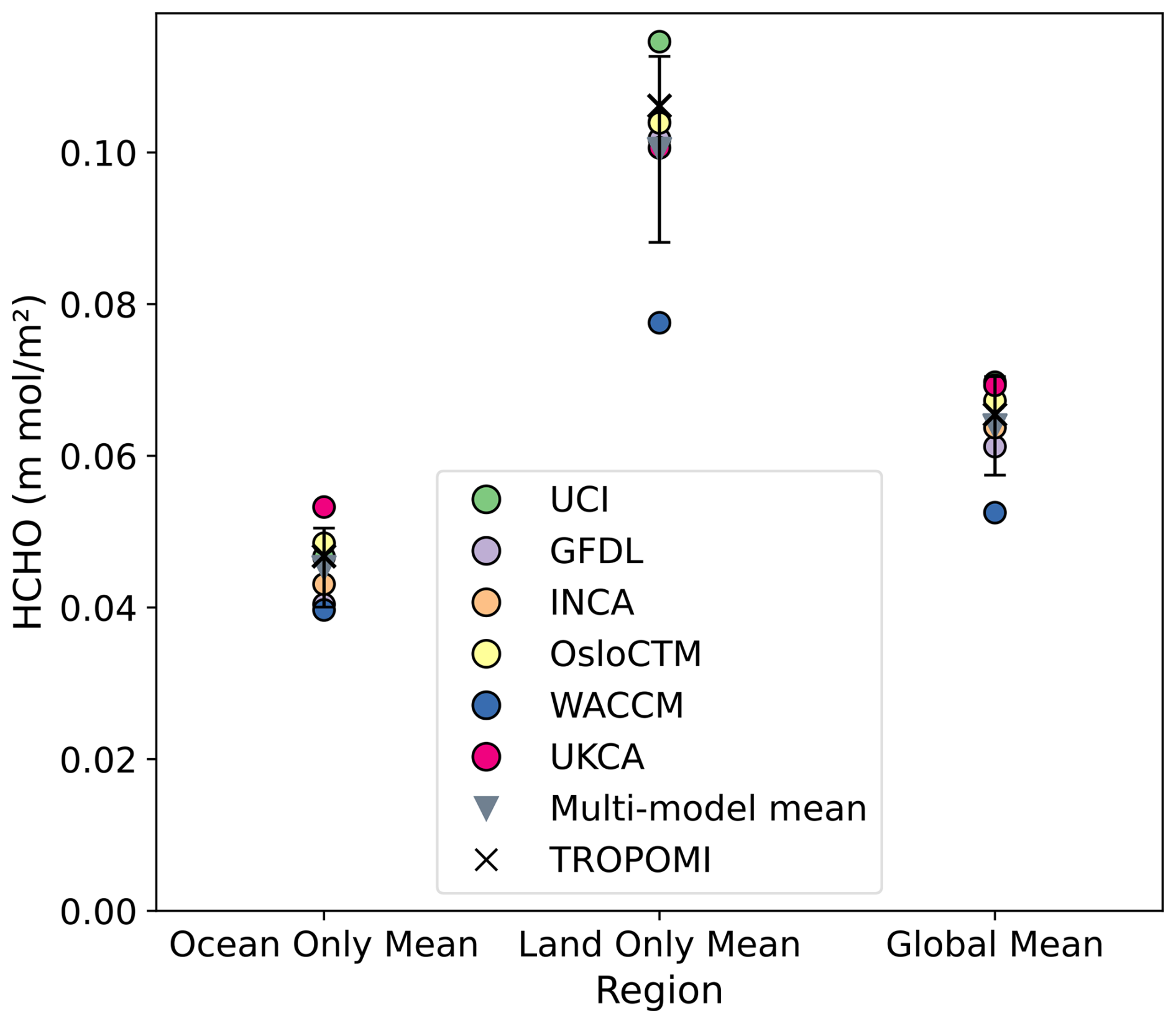
Figure A1 Comparison of annual mean formaldehyde over ocean, land, and global from TROPOMI satellite retrievals for July 2018–June 2019 (black crosses), six different ACMs (colored circles) and the multi-model mean (inverted triangle). The error bars correspond to the standard deviation from the model mean.

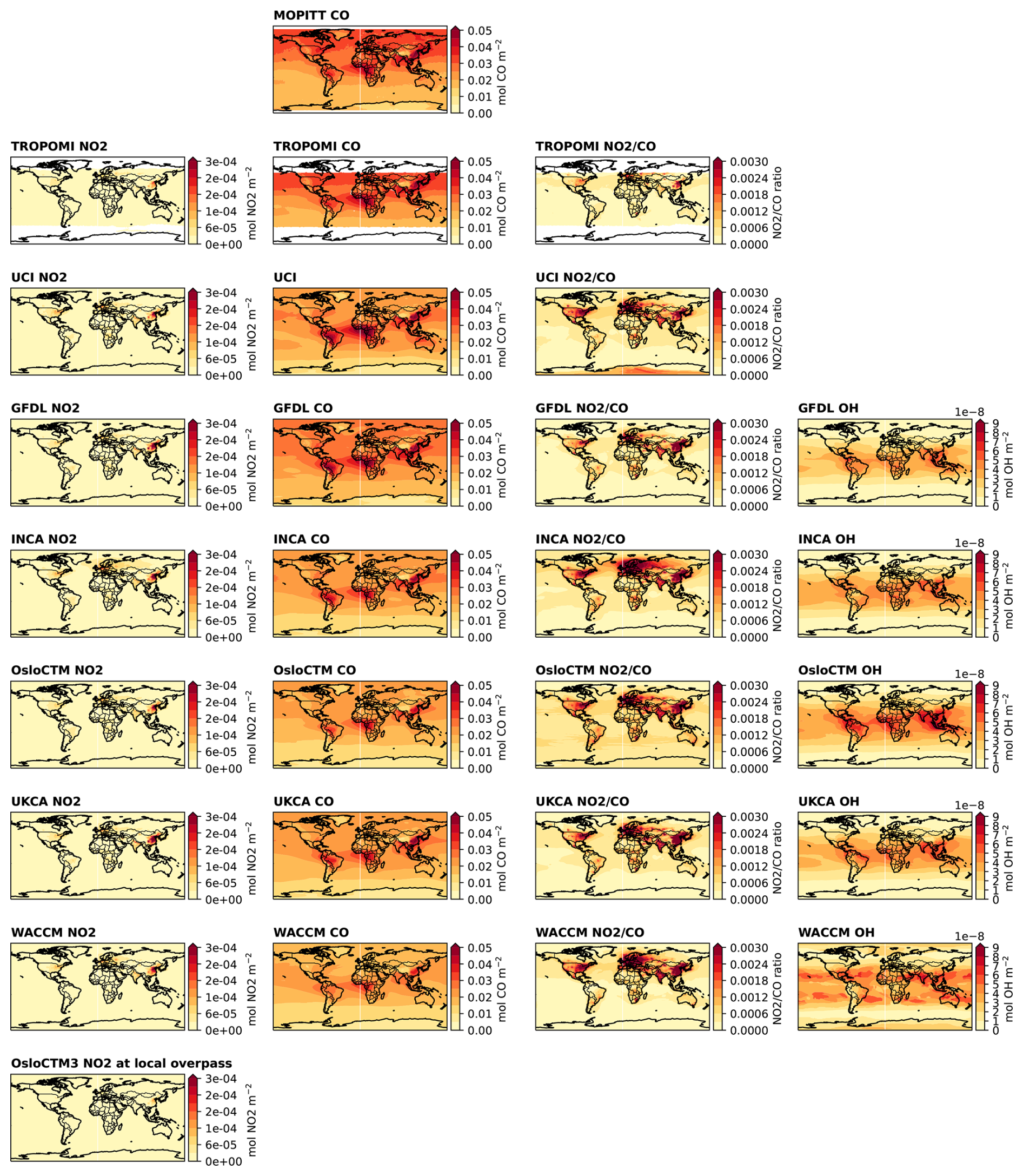
Figure A2 Global maps of annual mean satellite retrievals for (a) NO₂ for TROPOMI and models; (b) CO for MOPITT, TROPOMI and models; (c) ${\mathrm{NO}}_{\mathrm{2}}/\mathrm{CO}$ values in the models, and (d) OH in the models other than UCI.

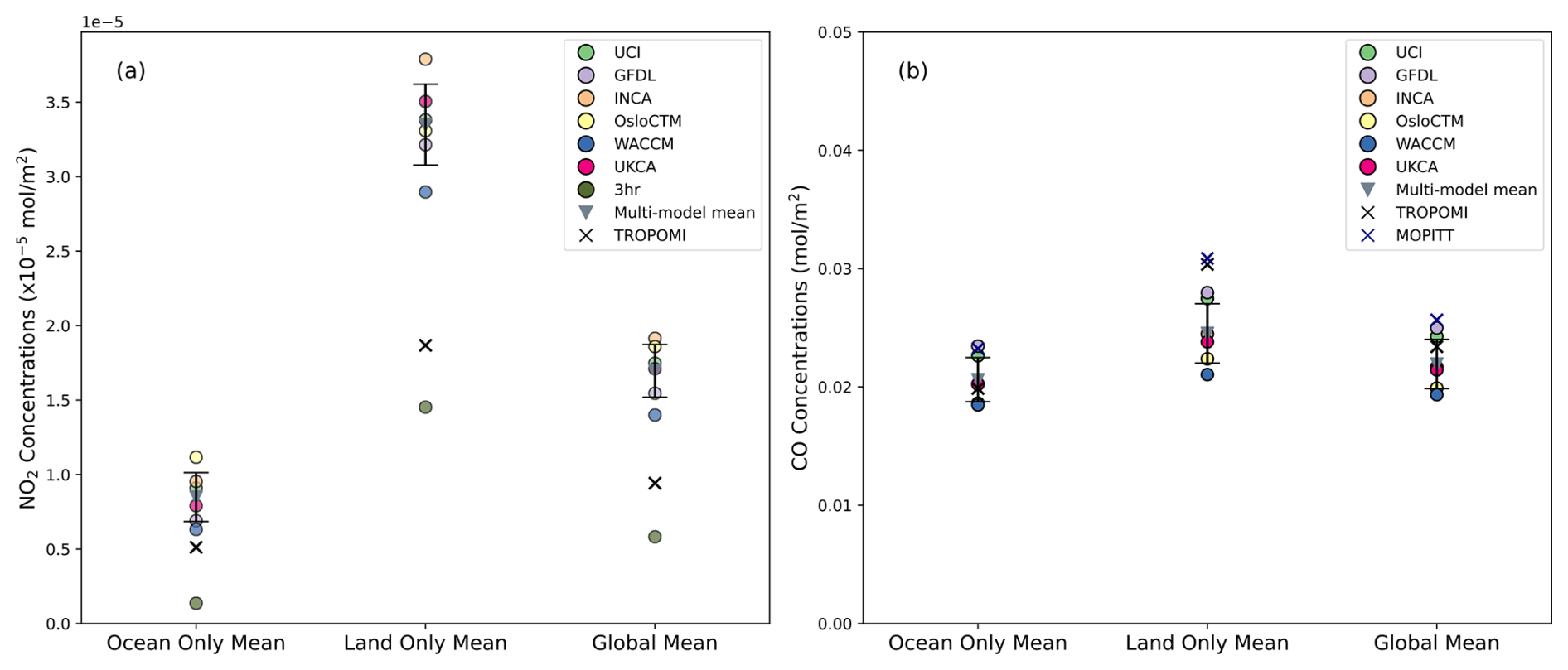
Figure A3 Comparison of annual mean (a) NO₂ and (b) CO concentrations over oceans, land, and global domains. Satellite retrievals from TROPOMI are shown as black crosses while MOPITT retrievals are represented by blue crosses. Colored circles denote results from the different ACMs, with the OsloCTM3 (3-hourly output) shown in dark olive green. The inverted triangle indicates the multi-model means calculated for model output with monthly means. The bars show the standard deviation for the multi-model means.

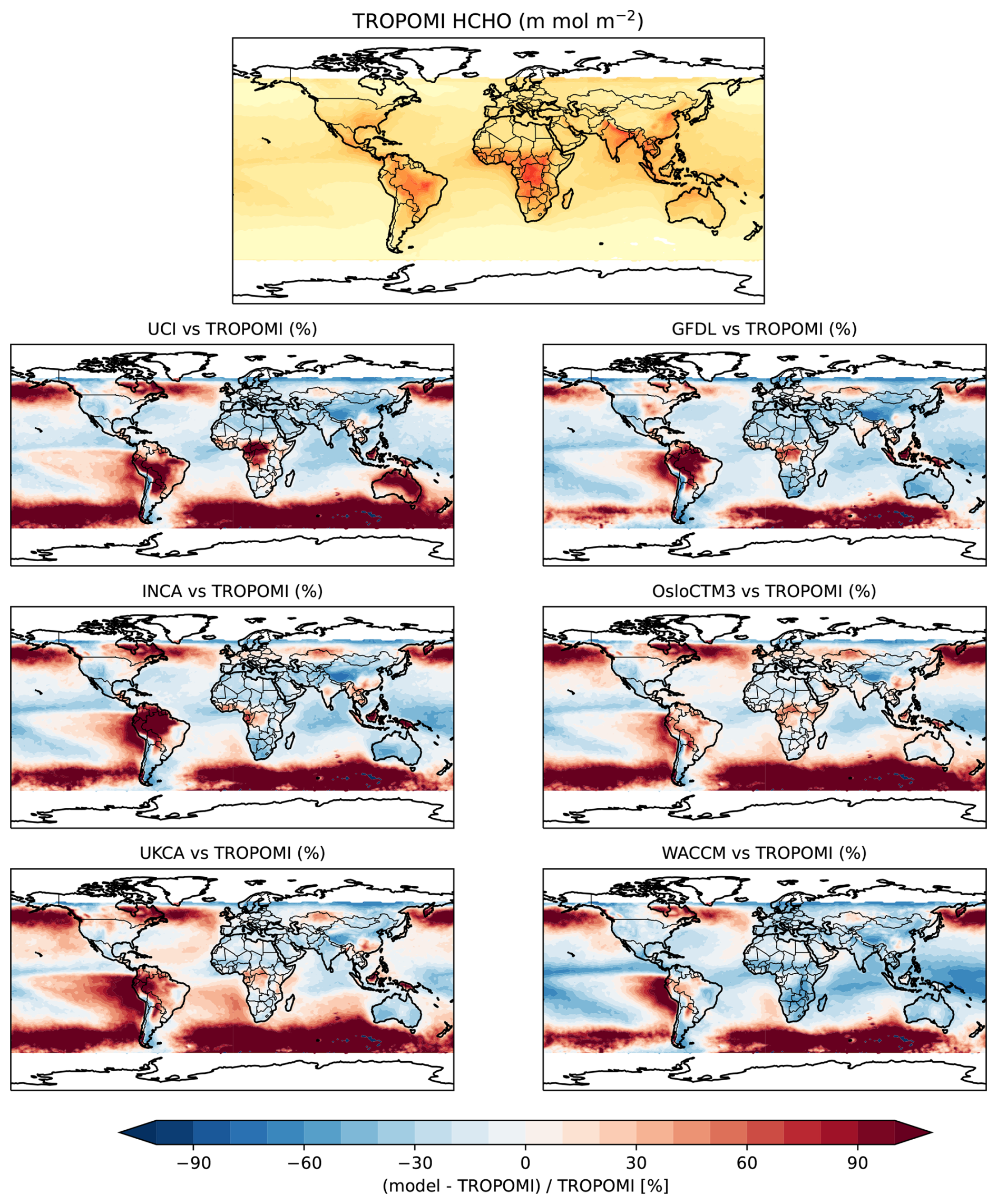
Figure A4 Percentage differences in HCHO between TROPOMI satellite data for July 2018–June 2019 vs. model simulations for 2010.

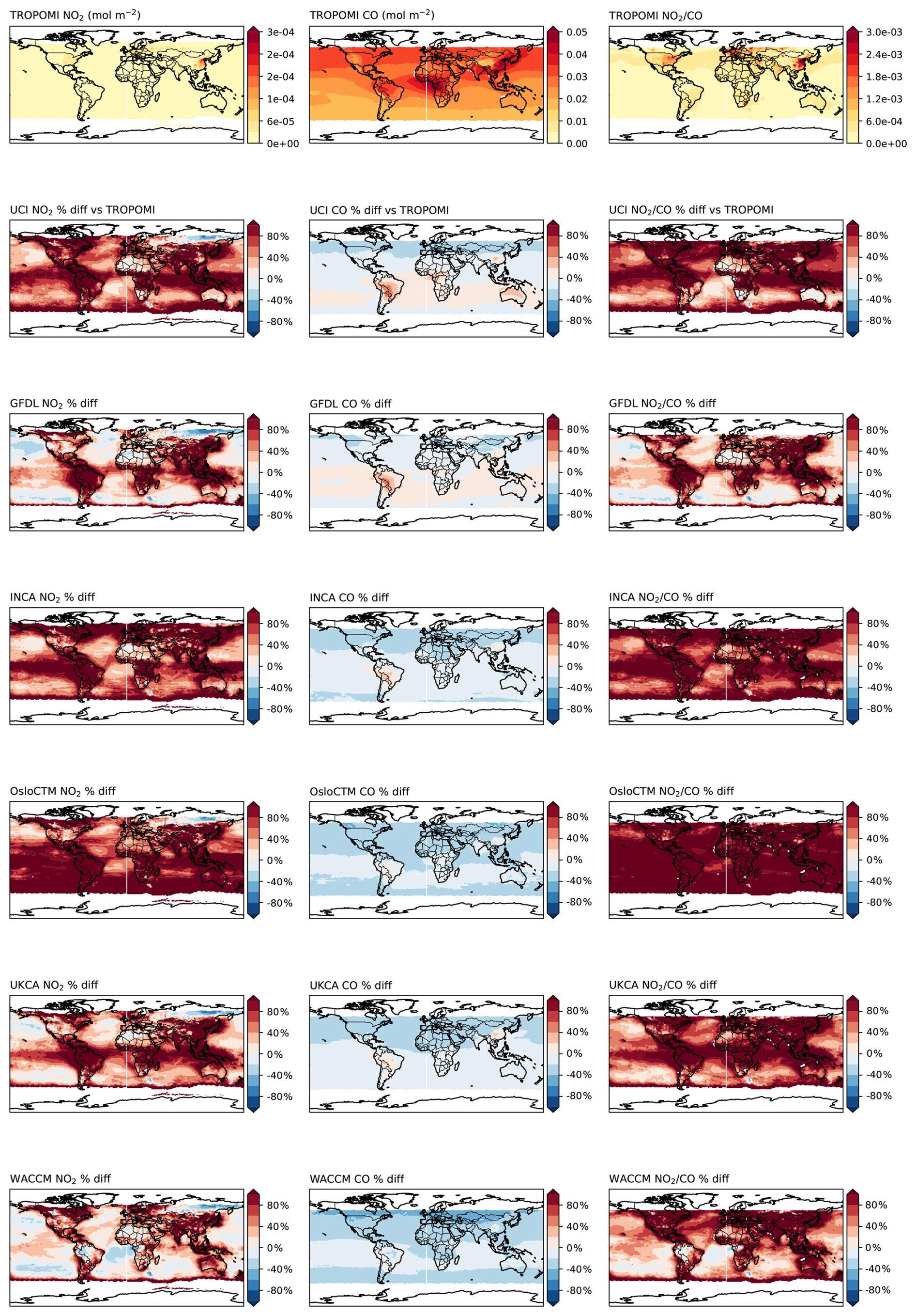
Figure A5 Percentage differences ((model − TROPOMI) $/$ TROPOMI) in NO₂, CO, ${\mathrm{NO}}_{\mathrm{2}}/\mathrm{CO}$ between TROPOMI satellite data for July 2018–June 2019 vs. model simulations for 2010.

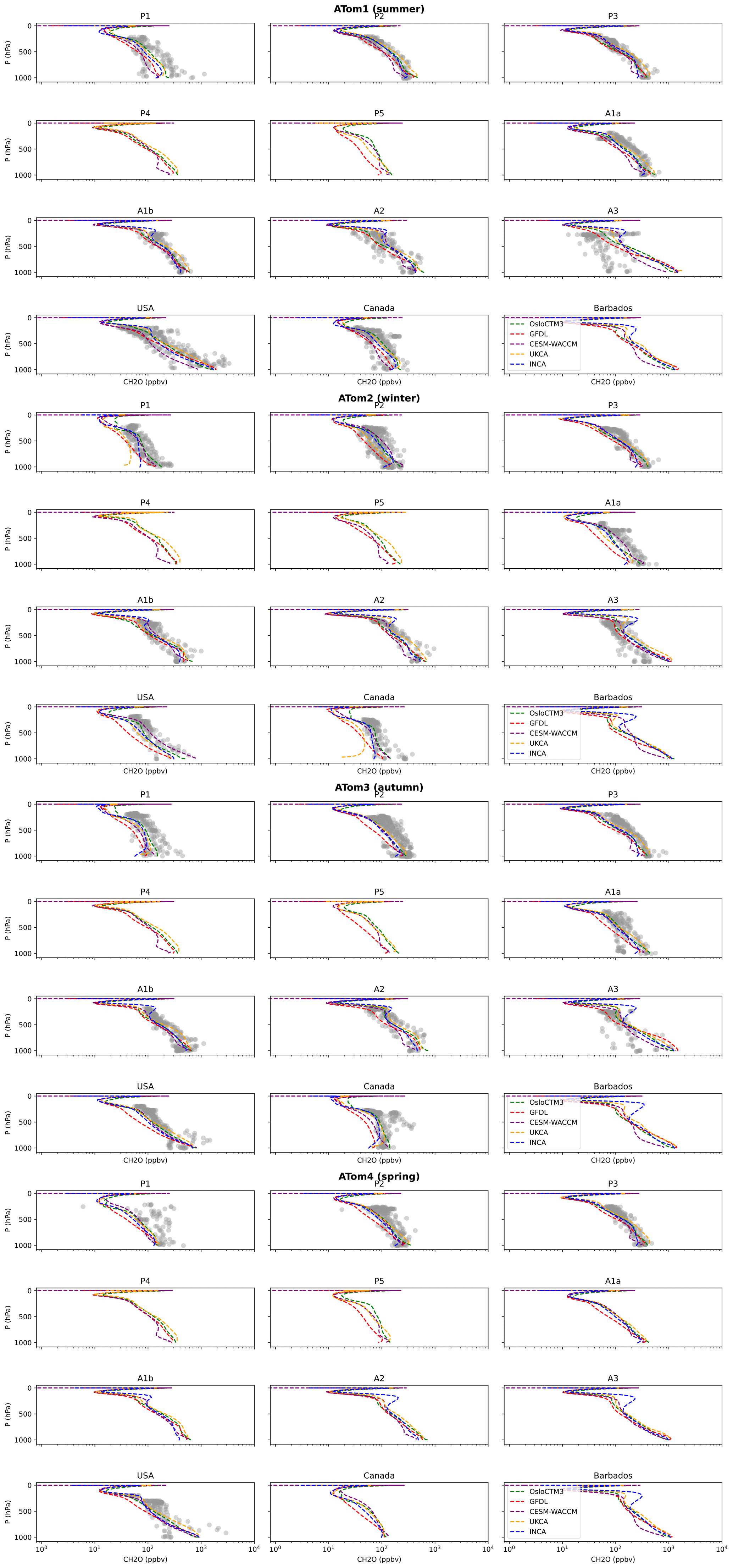
Figure A6 Vertical profiles of formaldehyde (HCHO) compared against observations from four different ATom campaigns. Each panel corresponds to a specific geographical box, defined by latitude and longitude bounds: P1 (180° W to 135° W, 60° N to 90° N): Polar North Pacific; P2 (180° W to 135° W, 30° N to 60° N): Mid-latitude North Pacific; P3 (180° W to 135° W, 0° N to 30° N): Equatorial North Pacific; P4 (160° E to 135° W, 30° S to 0° S): Equatorial South Pacific; P5 (160° E to 135° W, 60° S to 30° S): Mid-latitude South Pacific; A1a (45° W to 10° W, 30° N to 60° N): Mid-latitude North Atlantic; A1b (45° W to 10° W, 0° N to 30° N): Equatorial North Atlantic; A2 (45° W to 10° W, 30° S to 0° S): Equatorial South Atlantic; A3 (65° W to 30° W, 60° S to 30° N): Western Atlantic; USA (135° W to 80° W, 30° N to 60° N); Canada (135° W to 45° W, 60° N to 90° N); Barbados (80° W to 45° W, 0° N to 30° N).

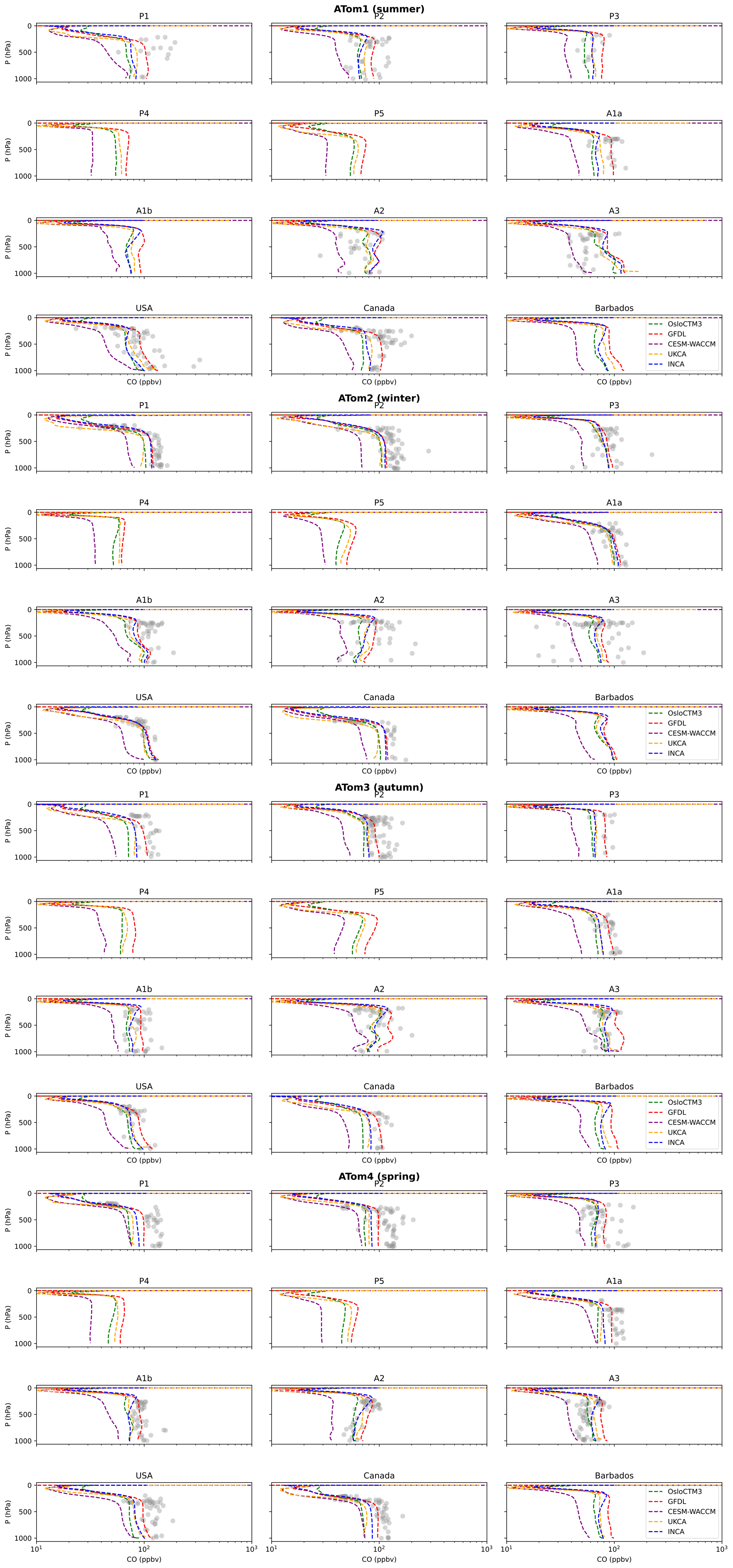
Figure A7 Similar to Fig. A6 but for vertical profiles of carbon monoxide against observations from the ATom campaigns.

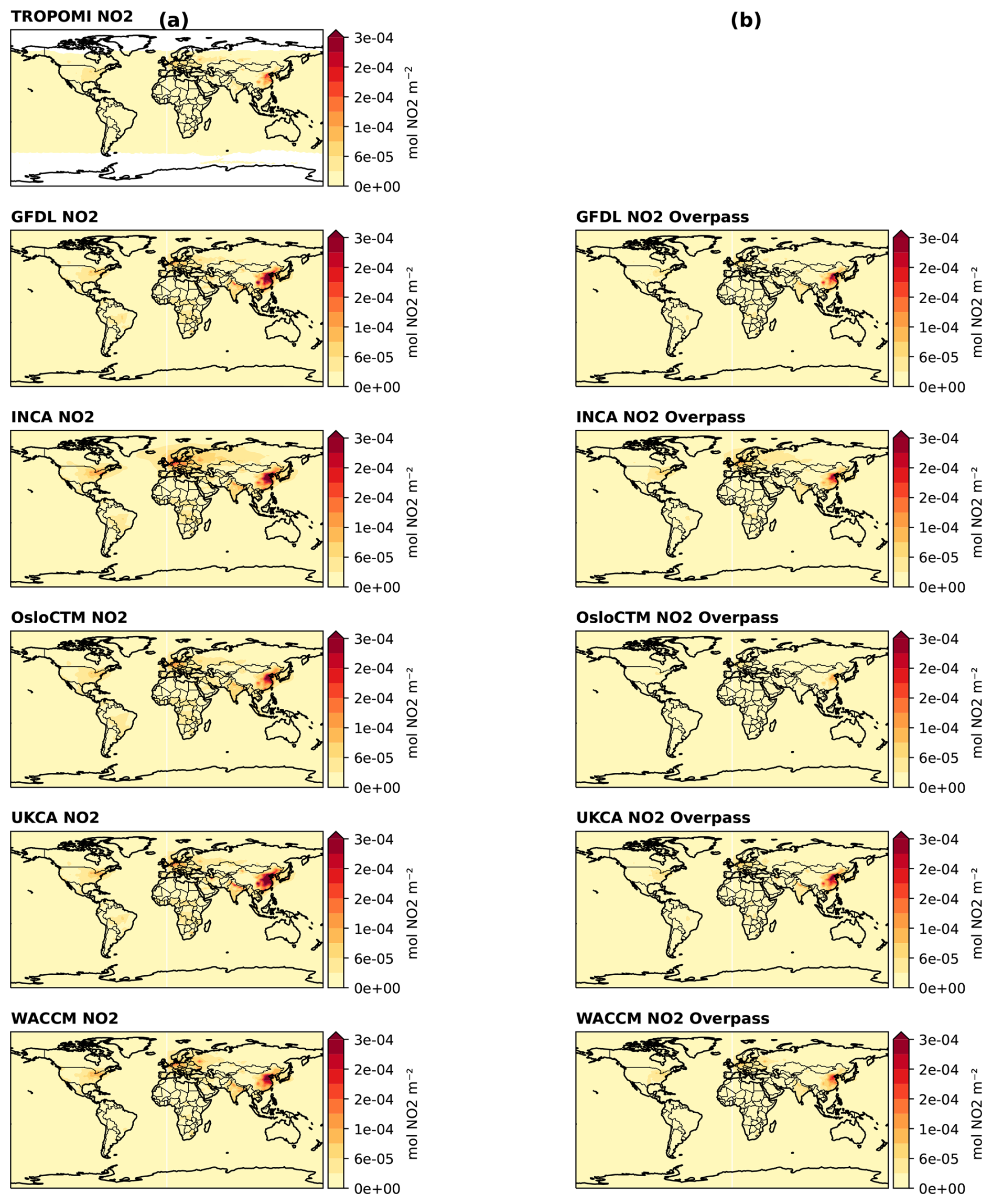
Figure A8 Global maps of annual mean satellite retrievals for (a) TROPOMI satellite retrievals for June 2009–June 2010 and annual mean model NO₂; and (b) model NO₂ during overpass for the models calculated as the product of monthly mean values with the ratio of monthly mean:3-hourly values during overpass for OsloCTM3.

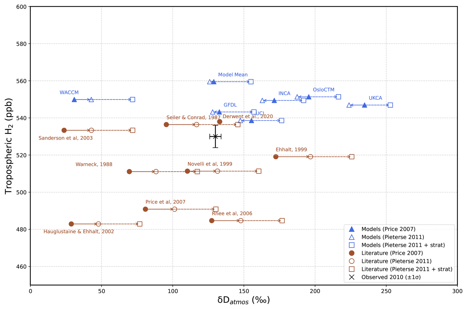
Figure A9 Similar to Fig. 8, but using isotopic compositions for sources and sinks from Pieterse et al. (2011) and 29 ‰ as stratospheric contribution.

Figure A10 Effect of different isotopic compositions for a geological source of 9 Tg yr⁻¹.

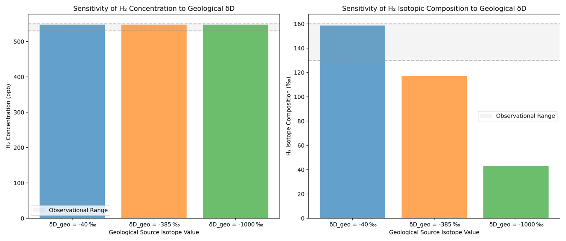
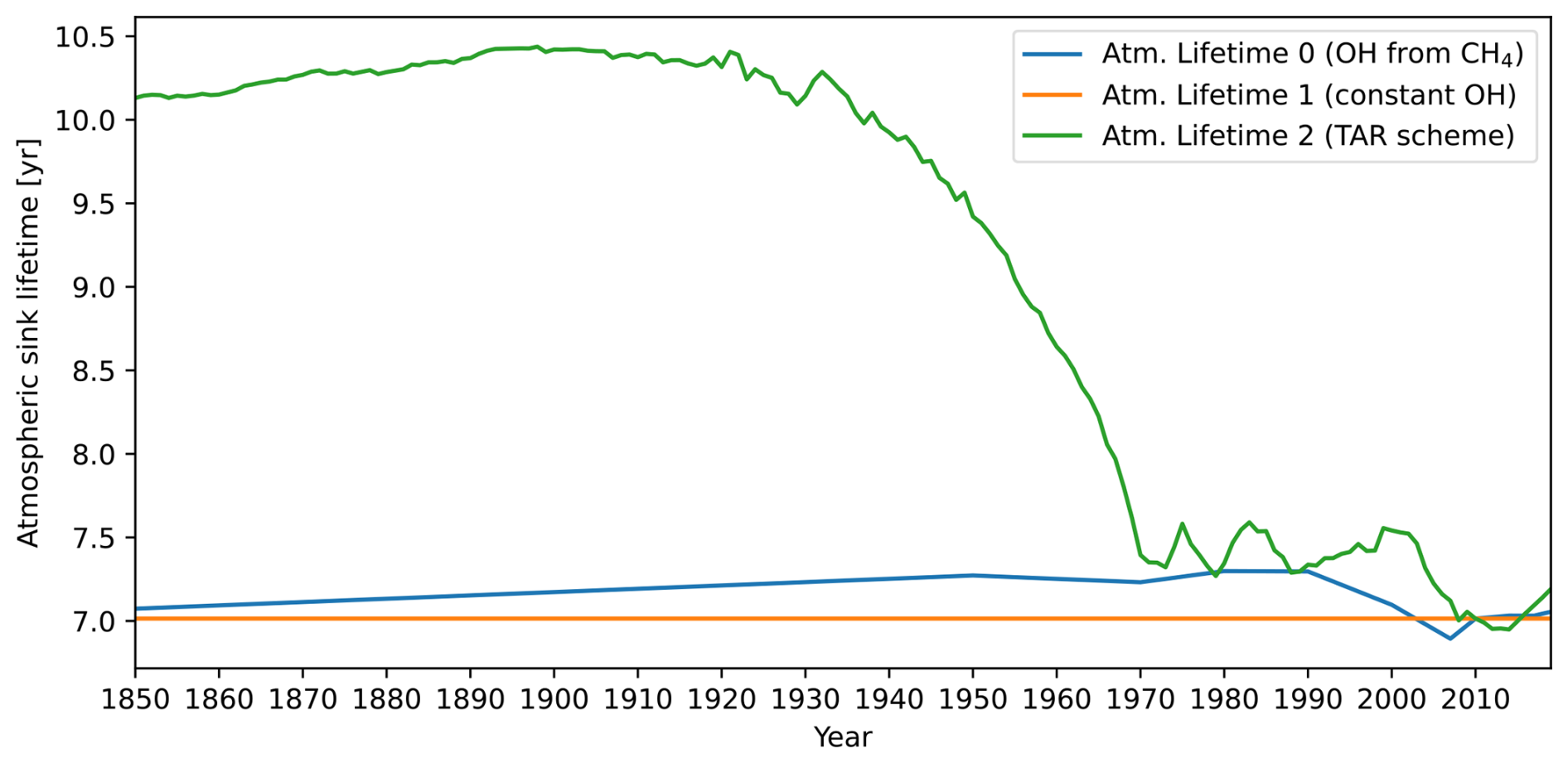
Figure A11 Different OH-sink lifetimes used in the box model simulations to test the effect of time varying OH-concentrations on the atmospheric loss. The three OH-based lifetimes are calculated as Atm. Lifetime 0: Time-variant OH based on trends in Stevenson et al. (2020) and Skeie et al. (2023a); Atm. Lifetime 1: Constant OH leading to constant atmospheric lifetime; Atm. Lifetime 2: time-variant OH using the following equation from the Third Assessment Report (Ehhalt et al., 2001): $\mathit{\delta }\ln \left(\text{tropospheric OH}\right)=\mathrm{-}\mathrm{0.32}\times \mathit{\delta }\ln \left({\mathrm{CH}}_{\mathrm{4}}\right)+\mathrm{0.0042}\times \mathit{\delta }\left(e\mathrm{-}{\mathrm{NO}}_x\right)\mathrm{-}\mathrm{1.05}\times {\mathrm{10}}^{\mathrm{-}\mathrm{4}}\times \mathit{\delta }\left(e\mathrm{-}\mathrm{CO}\right)\mathrm{-}\mathrm{3.15}\times {\mathrm{10}}^{\mathrm{-}\mathrm{4}}\times \mathit{\delta }\left(e\mathrm{-}\text{VOC}\right)$, where CH₄ is in ppb and the (e−X) is in Tg of species X per year.

Table A1 Parameter and input data for the box model. Values in this table is for the setup where the box model is adjusted to OsloCTM3 results from Sand et al. (2023). The model can be adjusted to other ACMs replacing OsloCTM3 values with values from Table 2.