Assessing raindrop evaporation over northern Western Ghats from stable isotope signature of rain and vapour

Stable isotopes of hydrogen and oxygen were analysed in rain and vapour samples collected simultaneously from Pune, India, during the 2019 summer monsoon. The δ¹⁸O and δD were significantly depleted in four events when the Outgoing Longwave Radiation showed a strong negative anomaly suggesting large-scale convection. The δ¹⁸O values of the rain samples are negatively correlated with their d-excess indicating effect of drop evaporation. Isotope exchange between rain and ambient vapour and associated raindrop evaporation in the sub-cloud layer, tracked by Δδ–Δd plot, suggest an equal share of equilibrium exchange and drop evaporation.

We used a one-dimensional Below Cloud Interaction Model (BCIM) to quantify sub-cloud processes affecting raindrop evolution. A Rayleigh ascent assumption in the BCIM simulations yields higher rain isotope values. Using radiosonde-based temperature and humidity profiles and constructing vapour isotope profiles from a combination of Tropospheric Emission Spectrometer data and a global circulation model (LMDZ) output, a better agreement is reached between the model and observed values. Sensitivity studies reveal that model values are strongly influenced by vapour isotope profiles, and moderately by drop size, temperature and relative humidity. Raindrop evaporation fraction estimated from the model yields daily-scale values varying from 4 % to 61 % (on average 23 %). This evaporation influences the heat budget and affects the monsoon convection. In addition, our study shows that drop evaporation reduces the rainfall amount considerably, especially in the lower range of precipitation. A precise quantification of raindrop evaporation is required for validation of the models used routinely for monsoon rainfall predictions.

1 Introduction

The Intergovernmental Panel on Climate Change (IPCC) has emphasized the importance of recycled moisture in the atmosphere (IPCC, 2014). Moisture recycling includes processes by which a fraction of the precipitated water returns to the atmosphere and causes further precipitation over the same area (Gray, 2012). These processes are soil evaporation, transpiration from plants, intercepted or condensed water on leaves, and evaporation from falling raindrops (Brubaker et al., 1993; Trenberth, 1999). This recycling increases with ambient temperature but decreases with humidity (Pranindita et al., 2022; Zaitchik et al., 2006; Zhang et al., 2021). It has been observed (Kumar et al., 2021; Pathak et al., 2014) that a high precipitation recycling ratio (∼ 15 %) pertains over India during the Indian Summer Monsoon (ISM; June–September). Among the contributing factors, raindrop evaporation is difficult to estimate because the parameters needed for estimating rain evaporation are not directly available from satellite sources.

Stable isotopologues (¹H${}_{\mathrm{2}}^{\mathrm{18}}$O, ¹H²H¹⁶O, ¹H${}_{\mathrm{2}}^{\mathrm{16}}$O) of rain waters can be used to assess the magnitude of raindrop evaporation (Crawford et al., 2017; Rahul et al., 2016; Salamalikis et al., 2016; Wang et al., 2021; Xiao et al., 2021). Falling raindrops exchange isotopes with the ambient vapour; this happens throughout the fall but occurs mostly in the unsaturated sub-cloud layer. The magnitude of this exchange, which alters the rain isotope ratios, can be used to quantify the extent of raindrop evaporation. Using satellite-based observations of vapour isotopologues (¹H²H¹⁶O and ¹H${}_{\mathrm{2}}^{\mathrm{16}}$O) and an isotope mass balance model, Worden et al. (2007) estimated that in the tropics, nearly 20 % of the mass of raindrops evaporates. However, they noted that the satellite data has limited temporal and spatial resolution. Therefore, estimating drop evaporation on a daily to monthly scale over a particular location is difficult using the satellite datasets. Raindrop evaporation has also been estimated from ground-based rain isotope observations and a set of empirical equations (Froehlich et al., 2008; Li et al., 2021; Wang et al., 2016; Zhu et al., 2021). However, it is a challenge to account for all cloud microphysical processes and their associated isotopic fractionations in a small set of empirical equations. Normally, these processes are considered for simulating rain isotope values in various General Circulation Models (GCM; Risi et al., 2019; Yoshimura et al., 2008; Stewart, 1975). But recent studies have shown that most of these GCMs fail to estimate raindrop evaporation correctly in tropical India (Nimya et al., 2022; Sengupta et al., 2023). This is possibly due to the coarseness of grid sizes used in these GCMs, which are inadequate to capture the region-specific complexities of processes controlling the evaporation. This necessitates controlled isotope observations and region-specific models for proper estimation of this parameter (Aemisegger et al., 2015).

Various approaches have been followed to estimate raindrop evaporation using paired observations of rain and vapour isotopes. For example, a bin resolved microphysical model was used to quantify drop evaporation during the Atlantic Tradewind Ocean–Atmosphere Mesoscale Interaction Campaign (ATOMIC; Sarkar et al., 2023). Graf et al. (2019), based on surface rain and vapour isotope observations in Zurich, Switzerland, developed a simple one-dimensional model (Below Cloud Interaction Model, BCIM) which considers various cloud microphysical processes during raindrop formation (condensation, vapour deposition, riming, etc.) as well as evaporative exchange processes within and below the cloud. This model simulates the isotopic evolution of an ice/liquid drop as it undergoes exchange processes while falling to the ground. However, being a one-dimensional vertical model, it does not consider any moisture advection and downdraft.

In the tropical Western Ghats (WG) region of India, shallow convective clouds are the dominant types (80 % of clouds occur below 4 km and 45 % below 2.5 km altitude) during the ISM (Konwar et al., 2014). Faster evaporation of smaller raindrops associated with intense rainfalls from these clouds provides significant positive energy feedback to form mesoscale convection (Konwar et al., 2014; Tao et al., 2012). A study of drop size distributions showed that raindrop evaporation prevails in the warm rain process occurring in this region (Murali Krishna et al., 2021). The current study investigates the applicability of the BCIM to predict rain isotopes and estimate raindrop evaporation in Pune, situated on the lee side of the WG, using paired observations of rain and vapour isotopes during ISM.

2 Experimental Methodology

2.1 Study area

Rainwater and vapour samples were collected from the ground level at the Indian Institute of Tropical Meteorology (18.53° N, 73.85° E), Pune during the summer monsoon of 2019. This region receives > 90 % rainfall during the ISM and is situated at the lee side of the WGs (Fig. 1). Rainfall in Western India occurs from mid-tropospheric low-pressure systems in several episodes, each of which usually lasts for 2–3 d. These systems are locked in place during these periods and fed by moisture derived from the Arabian Sea (Ding and Sikka, 2006; Rao, 1976). The geographic location of the region, its altitude, rainfall variation across the WG mountains, and the topographic profile across Pune are shown in Fig. 1. There is a sharp variation of rainfall across the mountains from the coastal zone (30 mm d⁻¹) to the lee side (12 mm d⁻¹) which is a characteristic of orography-induced rainfall (Fig. 1). The surface air temperature in Pune varies from 20 to 30 °C during the ISM (Pattanaik et al., 2019).

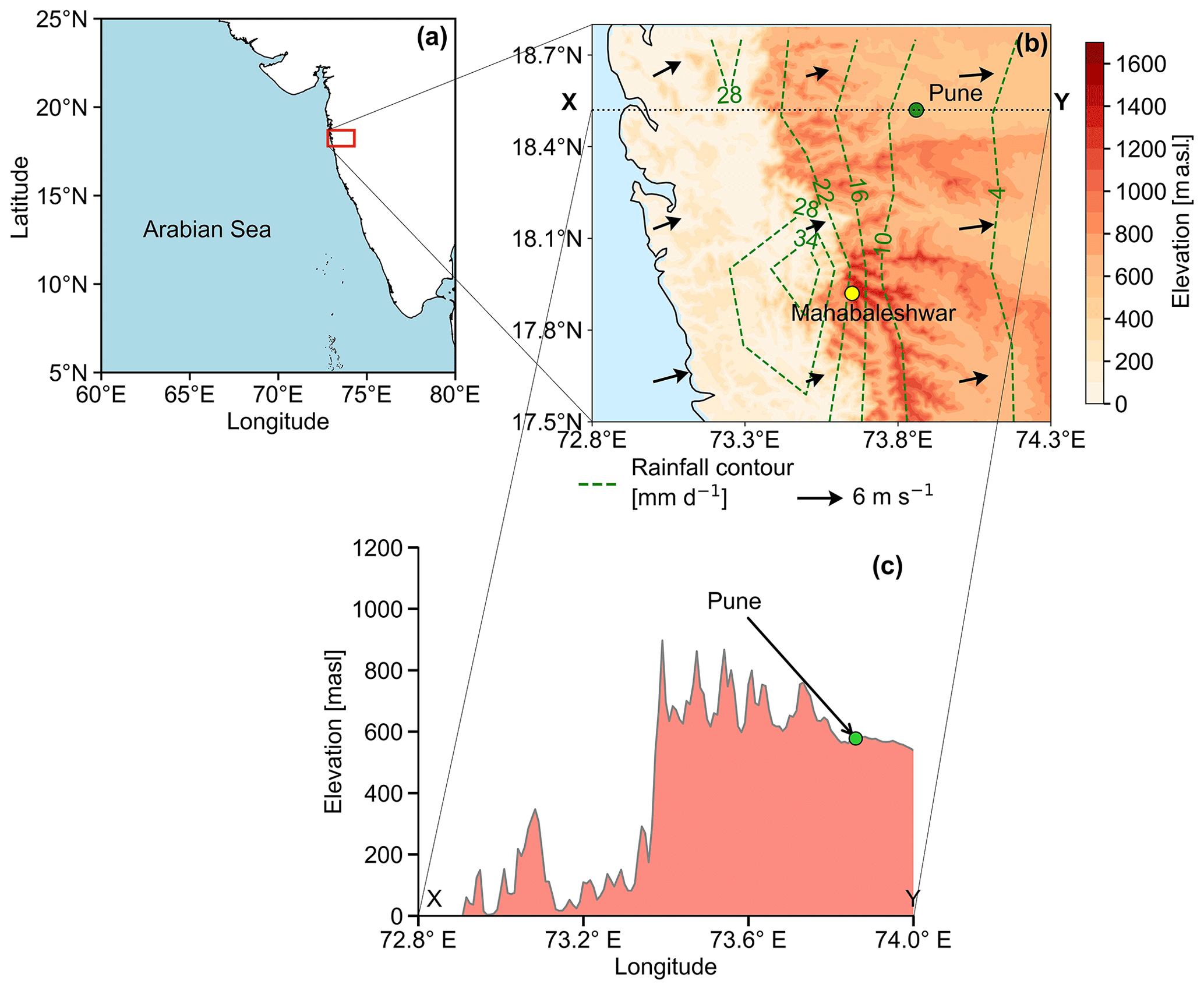
Figure 1 (a) The location of the study area in India. (b) Topographic map of the northern Western Ghats, India (prepared based on the GTOPO30 digital elevation model). The rainfall contours (long-term mean June–September rainfall in mm d⁻¹) were constructed using gridded (0.25° × 0.25°) rainfall data (1901–2020) from the India Meteorological Department (IMD). (c) A topographic profile along the latitude 18.53° N through Pune (Green circle at an altitude of 560 m) shows its position.

2.2 Sample Collection and Isotope Measurements

The onset and withdrawal dates of ISM (based on wind direction, specific humidity, and Outgoing Longwave Radiation, OLR; IMD, 2019) at Pune in 2019 were 22 June and 4 October 2019, respectively. Rainwater samples were collected during this period following the guidelines of the International Atomic Energy Agency (see Sect. S1 and Fig. S1 in the Supplement). For vapour samples, an in-house fabricated glass condenser was used (see Sect. S2 and Fig. S2). Twenty-nine vapour samples were collected during the rainy days, along with the rain samples; additional 14 vapour samples were collected during non-rainy days. The vapour collection efficiency was estimated from the amount collected against the amount expected (see Table S1 in the Supplement). Due to logistical problems, vapour samples could not be collected before mid-July.

The samples (rain water and condensed vapour) were measured using a Liquid Water Isotope Analyser (Model Number TIWA-45-EP, Los Gatos Research). This instrument measures liquid samples using Off-Axis integrated cavity output spectroscopy (OA-ICOS) with a routine precision of 0.1 ‰ and 1 ‰ for δ¹⁸O and δD, respectively, relative to VSMOW (Rajaveni et al., 2024; see also Sect. S3). The d-excess values defined as: d-excess = δD − 8⋅δ¹⁸O (Dansgaard, 2012) have a precision of 1 ‰. The rain isotope value of a particular day is reported after being weighted by the rainfall amount on that day.

2.3 Ground-based meteorological, Radiosonde and Satellite data

Daily average temperature, relative humidity and cumulative rainfall data were obtained from the Pune observatories of the IMD, available at the National Data Centre (https://dsp.imdpune.gov.in/, last access: 20 May 2025). The daily gridded data of zonal and meridional wind, specific humidity, air temperature, and cloud liquid water content were obtained from the European Centre for Medium-Range Weather Forecasts Reanalysis (ERA5) dataset with a resolution of 0.25° × 0.25° (Hersbach et al., 2020) and the Interpolated Outgoing Longwave Radiation (OLR) data (2.5° × 2.5°) were taken from NOAA (https://psl.noaa.gov/data/gridded/data.olrcdr.interp.html, last access: 3 December 2025).

The upper-air radiosonde data (relative humidity, RH; temperature, T) over Pune were obtained from the University of Wyoming repository (http://weather.uwyo.edu/upperair/sounding.html, last access: 29 January 2026). The values at every 50 mb interval (∼ 470 m in height) were available for two time periods: at 00:00 and 12 UTC, yielding two profiles for each day. The two profiles for each parameter (RH and T) were averaged to make representative daily profiles. Since the input for BCIM is required at every 1 m interval, a linear interpolation between two consecutive pressure levels in logarithmic scale (Ingleby et al., 2016) was carried out. However, the zone between the cloud base (Lifting Condensation Level, LCL) and the drop introduction height (taken as the height of Cloud Liquid Water Content, CLWC peak) poses a problem. As the BCIM requires 100 % RH for the formation of water droplets, the RH values above the LCL and up to the CLWC peak were considered as 100 %, disregarding the radiosonde data above the LCL (see Sect. 2.4.2). The typical uncertainties of T and RH are 0.3 °C (Sapucci et al., 2005; Jensen et al., 2016) and 8 % (Xu et al., 2023) respectively.

Tropospheric Emission Spectrometer (TES) Level 2 (Nadir-Lite-Version 6) retrievals of HDO and H₂O data for the available period (2005–2007) are used to construct mean vapour δD (δD_v) profiles (discussed later). The details of quality control criteria and biases associated with TES observations are discussed by Herman et al. (2014) and Worden et al. (2011). Grid point observations of δD_v have a precision of ∼ 10 ‰–15 ‰, which reduces to 1 ‰–2 ‰ when the data are averaged over a larger region (Lee et al., 2011; Pradhan et al., 2019).

To identify the moisture sources for vapour/rain at and around our study area, 48 h air mass back trajectory analysis was carried out at 850 mb pressure level using the NOAA Hybrid Single-Particle Lagrangian Integrated Trajectory (HYSPLIT) model (Draxler and Hess, 1997). The model tracks the movement of air parcels backward from a given location for a desired period (see Sect. S4 and Fig. S3).

2.4 The input parameters for BCIM

As mentioned earlier, to quantify the sub-cloud processes altering the rain isotope values, we used the BCIM (Graf et al., 2019). A brief description of this model, for application to the shallow cloud processes over Pune, is provided here. The model comprises a single vertical column that extends from the ground level to the point at which a single hydrometeor is introduced. Within this column, the hydrometeor descends under the influence of gravity, undergoes growth or evaporation (depending upon the ambient humidity and temperature), changes its isotopic composition through equilibrium and kinetic isotope exchange with surrounding vapour, and finally reaches the surface as a raindrop. The final isotopic composition of the drop is estimated by the following procedure: (1) setting up the initial condition involving the drop introduction height and its size, (2) estimation of the initial isotopic composition of the hydrometeor, (3) tracking the microphysical evolution of a falling hydrometeor, and (4) tracking the changes in isotopic composition of the hydrometeor along the descent. For these calculations, the model requires altitude profiles of T, RH and vapour isotopes for a given day as input parameters. The drop is assumed to form in equilibrium (at RH = 100 %) at a level which changes from day to day. The input parameters for the vapour can be introduced into the BCIM in two different ways: (1) the profiles can be calculated based on assumption of idealized (moist) adiabatic ascent of an air parcel from the surface to the top of the column; RH, T and vapour isotope values at various pressure levels are then estimated from the Rayleigh distillation equations starting from the measured surface values or (2) the height specific values of RH and T from radiosondes and vapour isotope values from satellite data and/or any model.

Since our aim is to understand the isotopic change and mass loss suffered by the drops due to rain vapour exchange, we introduce two parameters indicating the deviation of the final rain composition at the ground from the ambient surface vapour (Graf et al., 2019). This is most clearly expressed by the difference between the isotopic composition of vapour in equilibrium with the rain samples (rain eq. vapour) and the ambient surface vapour defined as: Δδ = δD (rain eq. vapour) − δD (surface vapour) and similarly for d-excess, Δd = d-excess (rain eq. vapour) − d-excess (surface vapour).

2.4.1 Drop size assignment

For calculating the dropsize change, the model requires the input diameter of the initial hydrometeor. Unfortunately, no disdrometer or micro rain radar observations were available for Pune during 2019. We, therefore, adopted the well-known Marshall–Palmer distribution (Marshall and Palmer, 1948), to estimate the mean drop size at the ground. First, we calculate the hourly mean drop size from the hourly rain rate, available from the IMD observatory at Shivaji Nagar, Pune, located about 4 km away from the sampling location. Next, we estimate the 24 h mean drop size by taking a weighted average of the size using rainfall amounts as the weights. The calculated drop sizes at the ground vary from 0.61 to 1.80 mm for the 29 sampling days. The drop diameter at the ground is next provided as an input, and the drop size at the drop introduction height (about 2.0 km above ground) is estimated iteratively in BCIM using the microphysics part of the model. This procedure was adopted for each day. The accuracy of the drop size based on the Marshall-Palmer distribution and the rain rate is limited, but this was the only option available to us. Our choice was guided by earlier modelling and observational studies where the Marshall-Palmer distribution has been used (Graf et al., 2019; Sarkar et al., 2023; Morrison et al., 2020; Ryu et al., 2025; Jiang et al., 2024).

2.4.2 Drop formation height assignment

In a simplified picture, the drop formation height corresponds to the most probable altitude range where the majority of the drops exist on any given day. However, this is not known a priori and was inferred from the analysis of CLWC data (see Sect. S5 and Fig. S4). The CLWC is defined as the total mass of liquid water droplets suspended in a unit volume of air within a cloud, typically expressed in grams per cubic meter or per kilogram of dry air. An earlier study by Kumar et al. (2014) showed that a peak of CLWC is often present at about 850 mb during the monsoon season over western India. In the present case, the CLWC profiles for 29 d of the study period, obtained from the ERA5 dataset, show peak values lying within 830 ± 70 mb, i.e., about 1650 m above mean sea level (see Table S2 and Fig. S4). Here, we consider the altitude of the CLWC peak of a given day as the drop introduction height for that day.

Clouds comprising small-sized water droplets form by condensation above a certain height where the vapour pressure equals the saturation vapour pressure. We can consider the cloud base height to be the Lifting Condensation Level (LCL) where RH attains 100 %. The RH and T profiles from the radiosonde data at various heights (see Sect. S5 and Fig. S5) can be used to estimate the LCL using the Skew-T–Log P diagram for all 29 sampling days. The LCL varies from 820 to 900 mb, and the average height is 890 ± 20 mb (about 1050 m; see Table S2). We notice that the LCL is always below the corresponding day's CLWC peak (by about 600 m on average) and therefore, the drop falls through a zone of 100 % RH till it emerges below the cloud base at LCL (see Sect. S5) where it falls through a zone of RH less than 100 %.

2.4.3 Isotopic composition of the ambient vapour and hydrometeor

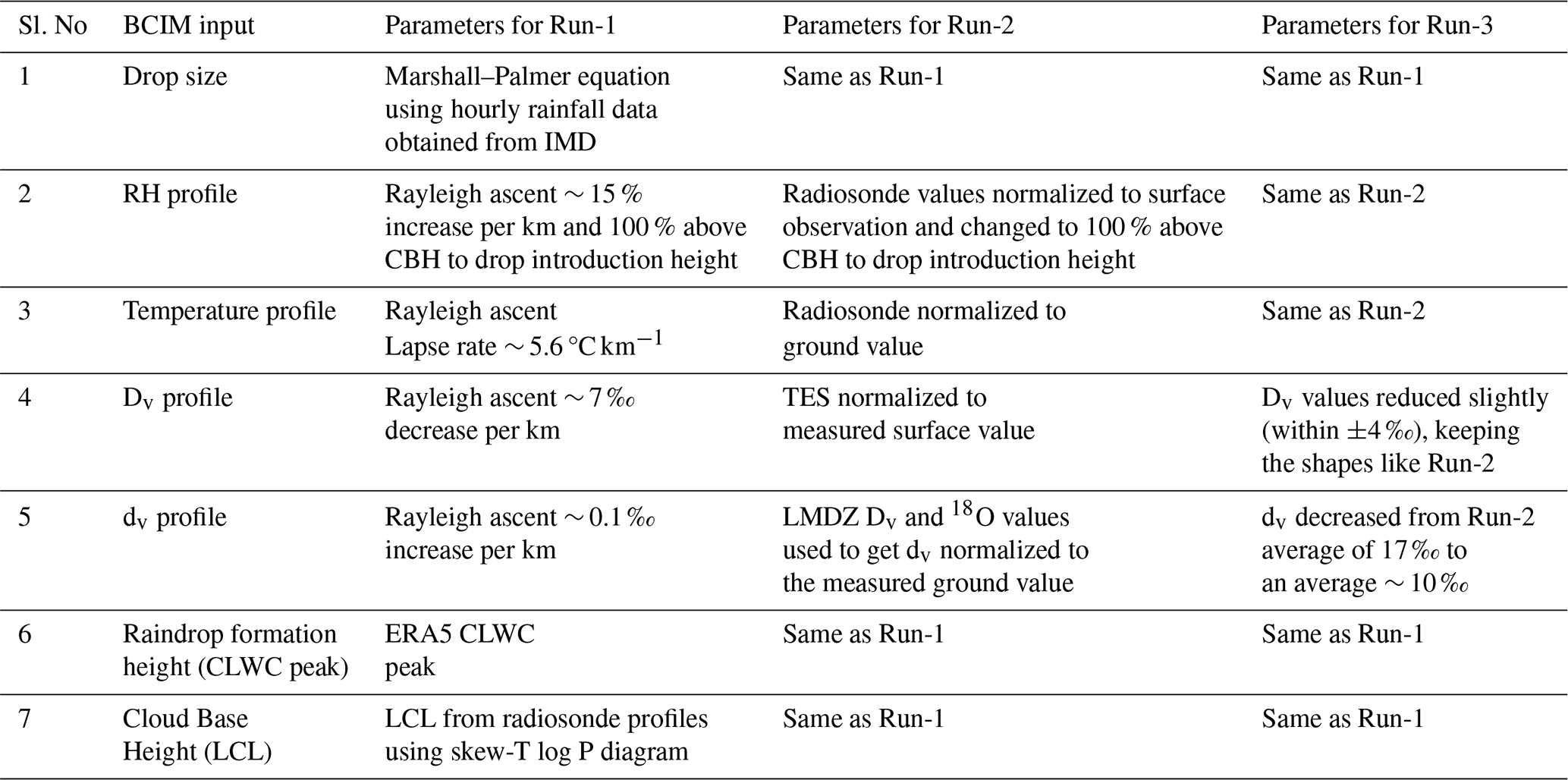
The isotopic composition of the ambient vapour at various heights is not known a priori. They are estimated from one of several possible sources and vary depending on the inherent assumptions. Three types of profiles were considered in this work, one after another, to improve BCIM predictions. To clearly present how this was done, we discuss the vapour isotope profiles along with the results for each choice in the Results section (Sect. 3.2.1 to 3.2.4; Table 1; See also Sect. S6).

Table 1 Input parameters for the three BCIM runs.

The initial composition of the introduced hydrometeor is calculated by assuming its formation in equilibrium with the vapour at this altitude and the ambient temperature. Subsequently, the composition of the falling hydrometeor at lower altitudes is calculated by using isotope mass balance and diffusive transport associated with isotopic exchange with the surrounding vapour (Graf et al., 2019).

The mass and temperature of the hydrometeor along its fall trajectory are calculated using the equations governing the microphysics of the falling hydrometeor (Foote and du Toit, 1969; Pruppacher and Klett, 2010). The temperature, pressure, and RH values are interpolated from the adopted profiles in various runs. It is important to mention here that many processes considered in the BCIM (e.g., ice formation, vapour deposition, rimming) do not occur for the shallow convective clouds in Pune (Utsav et al., 2017). Therefore, only relevant processes like condensation, isotope exchange, evaporation are considered in the present study (see Table 1). The BCIM also does not consider downdraft or advection of air masses. We obtain the inputs for various simulations from several sources listed in Table 1 and discussed in Sect. 3.2.

3 Results

We present the results of the current study in two main sections: (1) results of isotope analysis and (2) results of BCIM simulations. The first section presents the measured isotope ratios in the context of meteorological parameters, whereas the BCIM simulations are compared with the measured values in the second section.

3.1 Results of isotope analysis

Measured rain and vapour isotope ratios (δ¹⁸O and d-excess) on a daily scale are plotted in Fig. 2a and b. The general pattern of variations in vapour δ¹⁸O (δ¹⁸O_v) and rain δ¹⁸O (δ¹⁸O_r) values is similar; both decrease significantly and consistently after mid-August. The vapour δ values are lower than the rain. In contrast, the d-excess values of vapour (d_v) are always much higher. The δ¹⁸O_r and d-excess (d_r) values of rainwater range from −10.8 ‰ to 1.5 ‰ and −2 ‰ to 12 ‰, respectively, while those of the vapour range from −19 ‰ to −9 ‰ and 10 ‰ to 30 ‰, respectively. The mean and 1σ standard deviation of δ¹⁸O_r and d_r values are −1.3 ± 2.6 ‰ and 4 ± 3 ‰, while those of the vapour are −12.5 ± 2.5 ‰ and 18 ± 5 ‰, respectively. The δ¹⁸O (Fig. 2a) and d-excess (Fig. 2b) time series show four interesting features: (1) for the four date ranges: 27–29 June, 24–27 July, 4–8 September and 19–27 September, significant and consistent decrease in isotope values are observed in both rain and vapour phases (marked 1, 2, 3 and 4 in Fig. 2a; no vapour data available for date range 1), (2) On 19 September, the vapour shows a sudden decrease (marked A in Fig. 2a), (3) there is a gradual decrease in vapour δ¹⁸O_v values and an increase in d-excess values with the progress of the monsoon, which is especially prominent in the later part, and (4) rain d-excess (d_r) values remain constant with time but δ¹⁸O of both rain and vapour start decreasing beginning from early September.

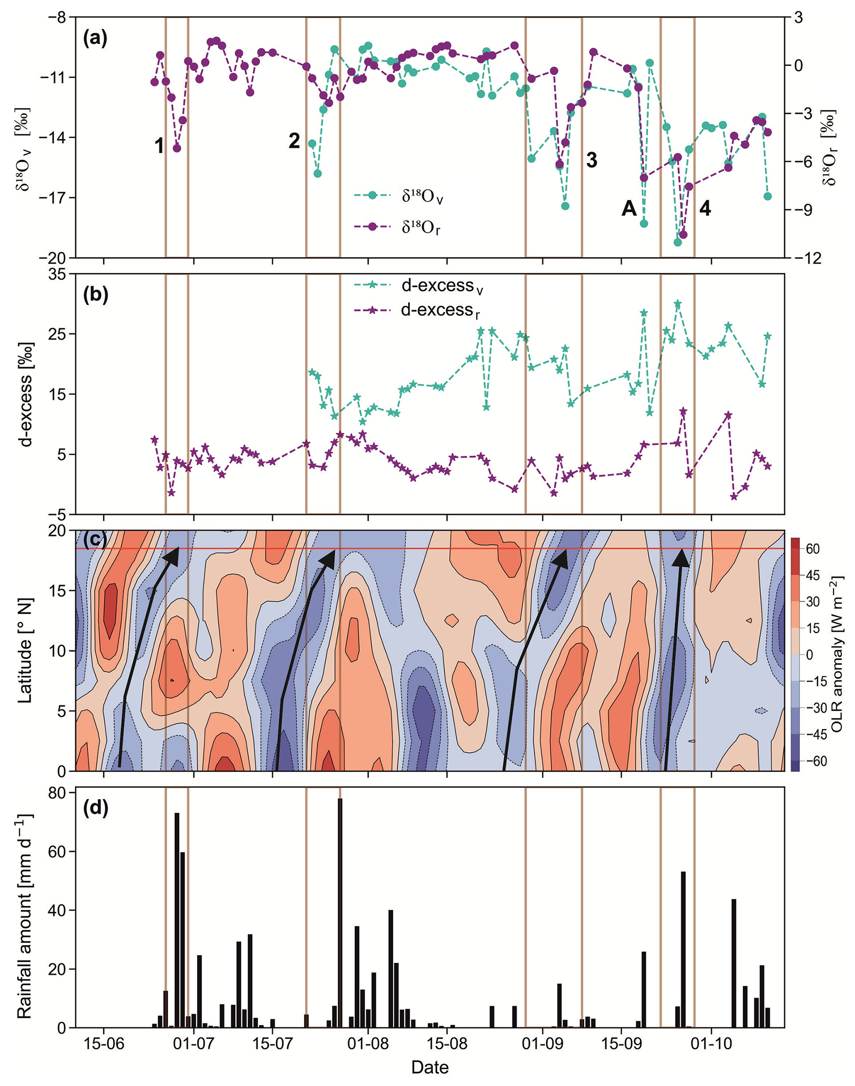
Figure 2 The time series of (a) δ¹⁸O and (b) d-excess values of the rainwater and water vapour, denoted by subscripts r and v, respectively. (c) OLR anomaly (W m⁻²) and (d) daily rainfall (mm over 24 h) in Pune. The four vertical boxes (numbered 1, 2, 3 and 4) denote synchronous periods of negative OLR anomaly values and low isotope values (i.e., less than their respective μ − 0.5σ values). These periods are defined as low-isotope events. Label A indicates one isolated low isotope value without associated negative OLR anomaly. Thick arrows show how convective cloud bands (indicated by low OLR anomaly) move to the sampling region in Pune from the southwest. Note highly depleted values on 19, 25 and 27 September. The red line in (c) indicates latitude of Pune.

Isotopic depletions in rain and vapour samples in the tropics are often associated with deep convection (Lekshmy et al., 2014; Risi et al., 2008; Sengupta et al., 2020). Signature of such a phenomenon is possibly present here in the form of depleted-isotope events when isotope ratios of a group of samples fall below the overall mean (μ) minus half the standard deviation (σ) (Sengupta et al., 2020). To find the relation of these events to large convective episodes, a latitude-time Hovmoller plot of daily OLR anomaly (averaged over the longitude 70–75° E) is examined in Fig. 2c. OLR values are often used as a proxy for convection because OLR is determined by cloud top temperatures which indicate cloud height. Consequently, a negative OLR anomaly corresponds to colder cloud top temperatures and greater cloud thickness which are characteristics of mesoscale convection. A time synchronous association of low OLR and depleted-isotope events thus indicate mesoscale convection affecting isotope values. Figure 2c indicates four such isotope-depleting mesoscale events (marked as 1, 2, 3 and 4 in Fig. 2a). In addition, we also see one depleted-isotope event without such association (marked as A in Fig. 2a). Interestingly, prominent second CLWC peaks occurred on 3 d, 19, 25 and 27 September, at much higher levels (about 550 mbar or about 5.5 km altitude; see Fig. 3) corresponding to the event number 4 mentioned above.

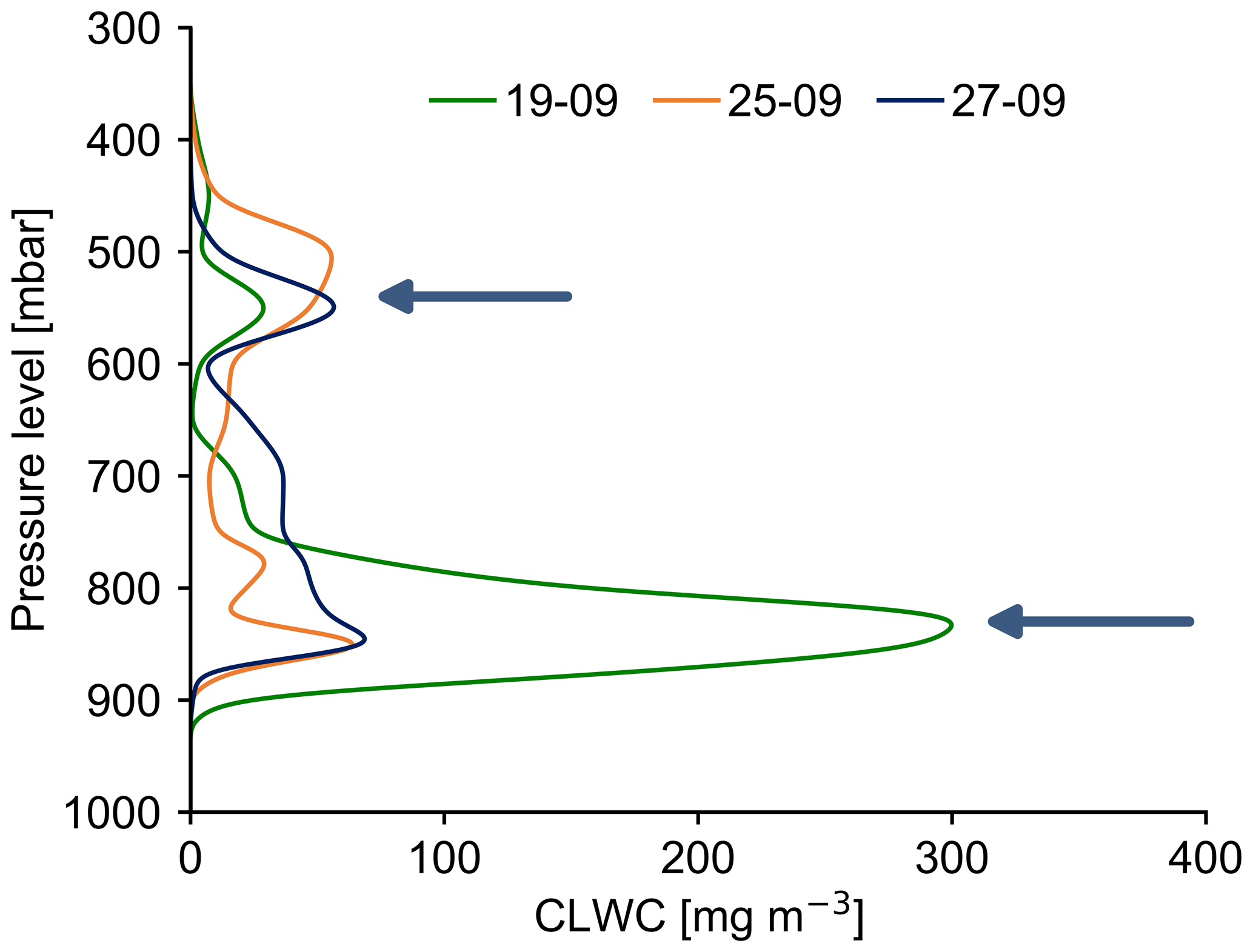
Figure 3 Presence of second CLWC peaks at higher altitudes (about 550 mb) on 19, 25 and 27 September 2019 (beside the first major peaks at lower altitudes) when highly depleted δ¹⁸O_r values were observed in association with negative OLR anomaly (see Fig. 2). The altitudes of the two sets of peaks are shown by two arrows. The data for the plot is obtained from ERA5.

Figure 2d shows that major rainfall occurred during the months of July and August. The relative humidity at the surface during the whole monsoon season varied from 71 % to 97 %, and the surface temperature varied from 25 to 30 °C (see Fig. S7). It is evident from Fig. 2d that deep convection is associated with high rainfall for the three events 1, 2, and 4. A recent study, based on a year-long continuous measurement of atmospheric vapour in Sri Lanka (a nearby tropical country with a similar monsoon system), also found such isotopic depletion during high rainfall events (Wu et al., 2025).

Figure 4a shows the Local Meteoric Water Line (LMWL) using rainwater samples and the Local Water Vapour Line (LWVL) using vapour samples from this study. The LMWL equation is δD_r = (7.3 ± 0.1) δ¹⁸O + (3.0 ± 0.3) and the LWVL, δD_v = (6.4 ± 0.2) δ¹⁸O − (1.9 ± 3.0), subscripts r and v denote rain and vapour. The slope and intercept of the LMWL values are lower than those of the Global Meteoric Water Line (GMWL), which are 8.0 and 10.0, respectively (Dansgaard, 2012; Gat, 1996). This difference, though small, suggests some amount of below-cloud evaporation of the rain. At Roorkee, a high-latitude Indian station, Saranya et al. (2018) found a LMWL with a lower slope (5.4) but a higher intercept (27). They attributed these changes to the contribution of evaporation from water bodies nearby and moisture recycling during the monsoon. Rahul et al. (2016) got a similar slope (7.4) but a lower intercept (1.5) in Bangalore (southern central India, at a high altitude of ∼ 1000 m). The lower slopes of meteoric water lines provide evidence of evaporation processes associated with kinetic fractionations occurring during rain evaporation.

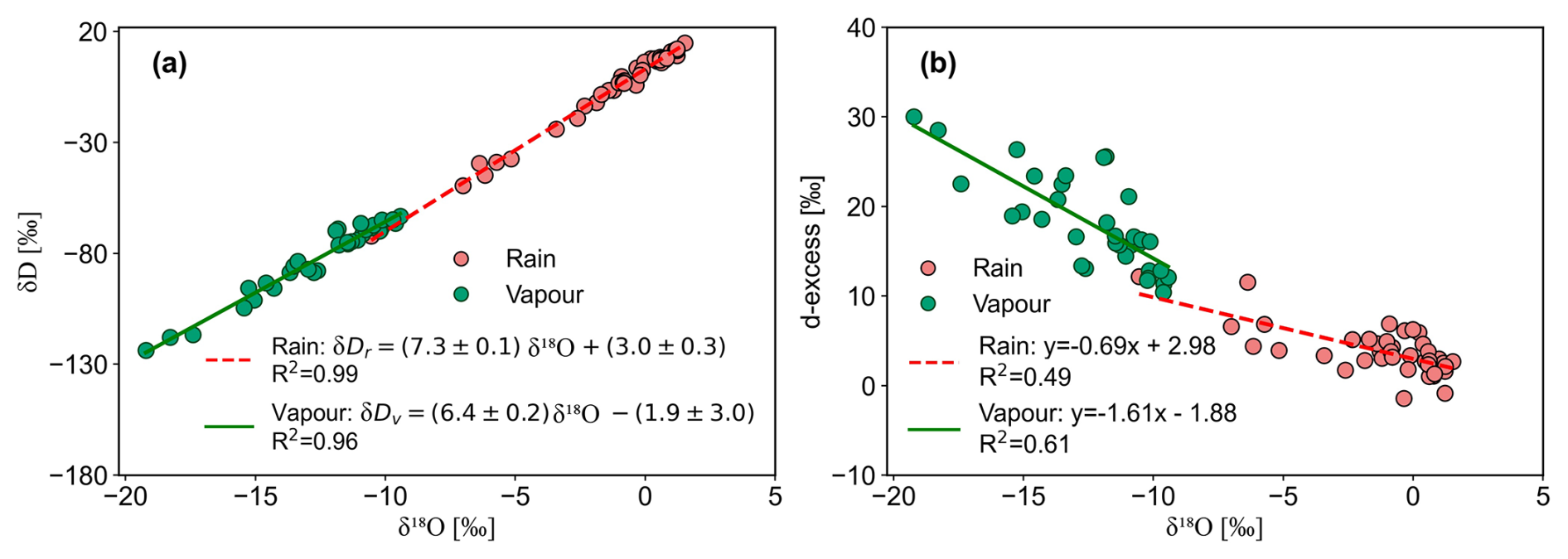
Figure 4 A cross plot of (a) δD and δ¹⁸O of rain and vapour. (b) A cross plot of d-excess and δ¹⁸O of rain and vapour showing anti-correlation. The regression equations and correlation coefficients are shown inside the plots.

The d-excess values of rain samples suffering evaporation generally bear a negative relationship with δ¹⁸O values (Bonne et al., 2014; Munksgaard et al., 2020). Such correlation is clearly seen in our data (Fig. 4b). In addition, the vapour d-excess values also show a statistically significant negative correlation with δ¹⁸O values (Fig. 4b; R² = 0.61; p = 0.001), probably indicating contribution of vapour derived from rain evaporation (Kurita, 2013; Risi et al., 2021). Correlation studies can be indicative, but the causative factors behind the above variations can be explored only with the help of a process-based model like BCIM.

3.2 Results of BCIM simulations

As discussed in Sect. 2.4, simulations of BCIM were carried out under three sets of initial conditions of RH, T and vapour isotope profiles designated as Run-1, Run-2 and Run-3. The aim was to achieve improvement in reproducing the measured rain isotope values by altering the input parameters step by step. The sources of input profiles of ambient temperature (T), relative humidity (RH), vapour δD (δD_v), and vapour d-excess (d_v) used for the three BCIM runs are given in Table 1.

3.2.1 Run-1: Rayleigh ascent results

In Rayleigh simulations (Run-1), the profiles were calculated using the equations for moist-adiabatic ascent of air parcels (following Appendix A1 of Graf et al., 2019), starting at the surface values of T, RH, δD_v and d_v of each sampling day as inputs. The values of δD_v and d_v were taken from our own surface vapour measurements, whereas the daily average T and RH values were obtained from the surface observations of IMD (Sect. 2.3). A dry adiabatic ascent formula is used up to the cloud base (LCL). Above the cloud base, a moist-adiabatic lapse rate is used. These input profiles for the 29 sampling days are given in Sect. S6.2 (Figs. S7 and S8).

Results of Run-1 (Rayleigh ascent) simulations are compared with the observed values of δD_r (Fig. 5a), δ¹⁸O_r (Fig. 5b), and d_r (Fig. 5c). We also construct Δδ − Δd cross plots for both observed and model values in Fig. 5d. Although observed and model isotope data (Fig. 5a and b) show strong correlation (R² = 0.86 and 0.79, respectively), the model values are significantly different (the plotted points deviate from the 1:1 line). The mismatched estimation of rain isotopes (δ¹⁸O_r and δD_r) affects the d-excess values considerably more; the points lie far to the right, and no correlation exists between the observed and model values (Fig. 5c). This is because the d-excess parameter is highly sensitive; even a small departure in δ values magnifies the discrepancy in d-excess. Most of the model values in the Δδ − Δd cross plot do not agree with the observed data points and lie closer to the origin. Many of the model points fall in the lower right quadrant, indicating prediction of strong raindrop evaporation. We also note that the model Δδ and Δd values (Fig. 5d) show smaller variations compared to the observations. The Δδ of the model simulations varies from 0 ‰ to 5 ‰ and Δd from 0 ‰ to −5 ‰, while the observed values have variations of about 25 ‰ (higher by a factor of 5). These comparisons show that the Rayleigh ascent model with the given inputs fails to reproduce the evolution of the rain isotopes in our region. It is evident that the vertical profiles of RH, T and vapour isotopes need to be modified to improve the simulations. The reason is not far to seek. Rayleigh ascent assumes that the source of vapour aloft is an unaltered rising air parcel with constant specific humidity. But we see from Fig. S9a and S9b that this condition results in unusually low cloud base over Pune (i.e., the level where RH attains the value of 100 %), inconsistent with observations (Naik et al., 2003). In fact, the radiosonde data show that specific humidity decreases with height (see Sect. S7; Fig. S9b). It is well known that a decrease in specific humidity is associated with a decrease in vapour isotope ratios (Noone, 2012; Worden et al., 2007; Fig. S9a). Moreover, in Run-1, the decrease of vapour isotopes with height is calculated using lapse rates starting from the measured surface δD_v and d_v. But these vapours are influenced by downdrafts associated with rain events. The downdrafted air brings down vapour with lower isotope ratios contributed by rain evaporation. Therefore, the post-rain vapour values are not representative of the atmospheric column before droplets form, precipitation falls, and rain evaporation occurs. To improve the model predictions, we need to change the profiles (see Run-2 results below).

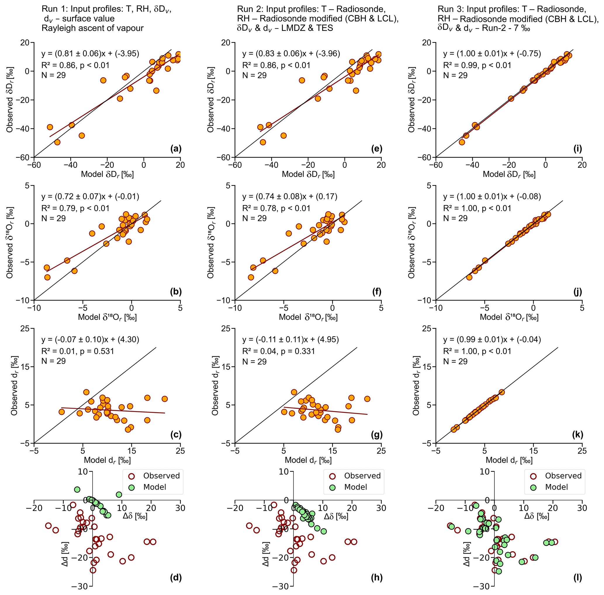
Figure 5 Scatter plots showing observed versus model values for rain δD_r, δ¹⁸O_r, and d_r for various runs (Run-1, Run-2 and Run-3) of BCIM in the upper nine panels. The bottom three panels show the Δδ − Δd cross plots for the runs. The sources of input profiles of T, RH, vapour δD_v and d_v used in the model for the three runs are given in the descriptions above. The best agreement between the observed and model values is achieved in Run-3. Run-3 uses the same RH and T as Run-2, but δD_v and d_v values are adjusted by tuning. The average d_v reduces to 10.7 ‰ from the value of 17.3 ‰ used in Run-2.

3.2.2 Run-2 results

The failure of the Rayleigh ascent method (Run-1) prompted us to explore other sources of vertical profiles of RH, T and vapour isotopes. RH and T profiles are now taken from the radiosonde (Sect. 2.3) and vapour isotope from TES as discussed below.

(a) Mean vertical profiles of vapour isotopes from TES and LMDZ

To obtain the vertical profiles of vapour isotopes, we first used an Isotope enabled General Circulation Model, LMDZ-iso (Risi et al., 2010). We obtained the GCM outputs over Pune for the sampling days from Dr. Camille Risi (personal communication, 2023). This model is a version of the LMDZ atmospheric model adapted to simulate the natural variations of water isotopes in precipitation and vapour. Unfortunately, when the vapour isotope values from LMDZ-iso over Pune are used as inputs to BCIM, the model values did not yield good agreement with observations (results not shown). Therefore, in the next attempt, we used the measured δD_v profiles obtained from Tropospheric Emission Spectrometer (TES) pertaining to the Pune region. However, the TES data were available only for 2005–2009. For our study year of 2019, we assumed that the time discrepancy can be accounted for if the final profiles are approximated by using the measured daily-scale surface vapour isotope ratios as a boundary constraint while maintaining the shapes of the TES δD_v profiles.

We should mention here that apart from TES, δD_v data, in principle, can be obtained from one other source, namely, the Atmospheric Infrared Sounder (AIRS) (see Sect. S8). However, isotope vertical profiles obtained from AIRS and used in the BCIM (after suitable boundary constraints) produced model rain values that were widely different from the observed values (Fig. S10). The possible causes for this are explored in Sect. S8.

The derivation of TES isotope profiles assumes that the shapes of the TES average profiles are applicable as far as the vertical variation is concerned. The TES satellite provides δD_v values of moisture at 17 pressure levels with a 5.3 km × 8.4 km footprint during the years 2005–2009 over a box covering the study region (16–20° N; 72–76° E). Using these data sets, we can derive an average TES profile and assume it to be representative of the shape of the mean ISM profile. Our station at Pune falls within the above-mentioned box, but we need to assume that the average over a ∼ 45 km² area represents the vapour over a small sampling station under the boundary constraint. With these assumptions, the TES average profile is adjusted so that its surface value matches the measured ground vapour value. A support for this assumption comes from the back-trajectory analysis that indicates that the Pune moisture source is always from the Arabian Sea (see Fig. S3). Interestingly, an average δ¹⁸O_r value of rainwater in Bombay (from 1961 to 1978) is −1.3 ‰ (Bhattacharya et al., 2003), close to the Pune average value of −1.1 ‰ from the present study. It shows that Pune, being located 150 km downstream of Bombay, receives moisture of similar composition as Bombay (with potential addition from the evaporation component on the way). Therefore, our assumption of a large spatial average representing a small location is not far from truth, at least as far as the vertical variation is concerned.

(b) Daily scale profile by adjustment technique

As mentioned, the δD_v and d_v profiles for each date were obtained from the TES data by adjustment with the measured surface values. We analysed the available TES δD_v profiles for the years 2005–2007 and derived three profiles which correspond to the minimum, mean and maximum surface δD_v values. Each of these three profiles was fitted with polynomials, and the coefficients of these polynomials were treated as functions of the surface values. Once we get these functions, we can obtain the vapour isotope profiles for any day by using that day's surface value. This exercise was necessary to translate the variation of the discrete TES values into an analytical form, allowing for easy calculation of vapour isotope values at each height (at one meter resolution) from the ground level to the drop introduction point.

A similar exercise was conducted to obtain the daily d_v profile from the LMDZ output and normalizing the profile to the measured d_v value for that date. In brief, this was done by using the available δD_v and δ¹⁸O profiles from LMDZ output for three cases (Mean, Max and Min surface values), fitting 4th-order polynomials: Ah⁴ + Bh³ + Ch² + Dh + E, and then constructing the d-excess profiles for three cases with five coefficients. Five coefficients were used to get higher precision in fitting. Again, fitting was done for each of the coefficients (A, B, C, D and E) as a function of surface value. Using the coefficients, d_v profiles are obtained for each day. This procedure is discussed in detail in Sect. S6.1. Figures S7 and S8 show the input profiles (RH and T), and (δD_v and d_v) respectively, for the three runs: Run-1, Run-2 and Run-3. The method of estimating the vapour profile, constrained by surface vapour measurements, assumes that the vapour aloft is related to the surface value. This assumption may not be strictly correct, but it allows us to check whether the BCIM, with the surface boundary constraints, yields better rain isotope ratios compared to the Rayleigh model while being consistent with the TES measurements of vapour aloft.

Finally, the above profiles were employed in BCIM (Run-2) to generate the daily-scale δ¹⁸O_r, δD^r and d_r values of rain samples (Fig. 5e–h). However, surprisingly, the results showed little improvement compared to Run 1 (Fig. 5e–g) although showing a larger variability in the Δδ − Δd plot (Fig. 5h); the Δδ values varied from −4.7 ‰ to 11 ‰ and Δd from −1.8 ‰ to −12.4 ‰. As in Run-1, all the model data points fell in the lower right quadrant of the Δδ − Δd cross plot (Fig. 5h and d). In conclusion, both Run-1 and Run-2 simulations fail to yield a good match with the model values (especially the d-excess). The δD_r values differ by about −8 ‰ to 20 ‰, and the model d-excess values are higher (by 0 ‰ to 15 ‰). Interestingly, the model rain values of Run-1 and Run-2 are quite close (within ±2.5 ‰; Fig. S11) despite RH, T, δD_v and d_v profiles being very different. This suggests that the assumption of surface vapour value as the boundary constraint, as used in both these runs, is the main determinant for rain isotopes.

3.2.3 Possible sources of failure in predictions of Run-1 and Run-2

The failure of Run-1 and Run-2 predictions, as discussed above, indicates that we still need to modify the input profiles to obtain a good match with the observed values. It is easy to see that the ambient vapour isotope values have the maximum impact on the model rain isotope values. This can be shown quantitatively by a multiple regression analysis of rain isotope values with four influencing factors (RH, T, surface D_v and drop diameter) in their normalized forms. The normalized values (the ratio of anomalies of the daily data and 1 standard deviation) of the model rain isotope ratios D_mod−rain obtained from Run-2 for the 29 sampling days were regressed with the normalized values of the above-mentioned four variables. We obtain the following multiple regression equation (normalized):

$$\begin{array}{}\text{(1)}& \begin{array}{rl}\mathrm{\Delta }{\text{D}}_{\mathrm{mod}-\mathrm{rain}}& =-{\mathrm{0.114}}^{*}\text{RH}+{\mathrm{0.035}}^{*}T\\ & -{\mathrm{0.059}}^{*}\text{drop diameter}+{\mathrm{0.986}}^{*}{\text{D}}_{\mathrm{v}}\end{array}\end{array}$$

This equation indicates that the major influence on the model rain isotope value is from the ambient vapour D_v (with a coefficient of nearly one, meaning +1 ‰ change in D_v would result in +1 ‰ change in the rain D_r). In contrast, the influence of RH, for example, is only one-tenth (in the opposite direction). The influences of T and droplet size are still less. It is logical to assume that the main source of discrepancy in Run 2 simulations is improper vapour isotope profiles and therefore, for tuning, a change in the vapour isotope value would be the most effective.

It seems that the true profile for a given date does not coincide with the adopted one based on extrapolating to the measured surface value, as assumed by the boundary constraint. In other words, the vapour aloft may not be derived entirely from the surface vapour as measured at our sampling location. The reason for this could be a significant contribution from the local moisture having a different isotopic composition (sourced from evaporation from various water bodies like lakes, rivers, ponds etc. or evapotranspiration from trees located within a few hundred meters). However, this possibility can be ruled out as a study using satellite data showed that, due to high humidity during the monsoon season, evaporation/evapotranspiration (∼ 0.5 mm d⁻¹) adds a negligible amount of moisture compared to the advective flux in this region (Pathak et al., 2014). In this context, we note that the measured surface vapour refers to post-rain ground-level vapour, which may suffer from downdrafted vapour with contributions from drop evaporation. This contribution may change the surface vapour when we measure it, making it different from the vapour that gave rise to the raindrops aloft. However, this suggestion is based on a posteriori reasoning and invoking downdrafted evaporation-generated vapour as a possible source is a speculation.

3.2.4 Run 3 results

Guided by the regression Eq. (1), we tuned the vapour δD_v and d_v input profiles (Run-3) to achieve a better agreement in the rain isotope values for each date (Fig. 5i–k). The surface δD_v values were changed by amounts varying from +13.9 ‰ to −17.8 ‰, and the d_v values from +3.2 ‰ to −17.1 ‰ while keeping the shape for daily profiles similar to Run-2. Corresponding changes in the vapour δ¹⁸O were from +2.9 ‰ to −1.9 ‰. Most of the changes were small; in the δD_v, 23 out of 29 changes were within ±4 ‰ and in the d_v 23 out of 29 changes were within ±3.4 ‰. As a consequence of this tuning, the average d_v of the surface vapour decreased to 10.7 ‰ from the average measured value of 17.3 ‰. The resultant vapour isotope profiles of Run-3 are shown (along with those of Run-1 and Run-2) in Fig. S8e, f. As designed, this tuning resulted in good agreement of the model values with the observed values. A two-tailed Student's t test shows that the Run-3 model values are close to the observed surface rain isotope values for all three parameters (δ¹⁸O_r, δD_r, and d_r) at p = 0.05 significance level (see Sect. S9; Table S3). The average (observation-model) d-excess difference decreases from 2.1 to 0.4. Additionally, there is a close match in the Δδ − Δd cross plot (see Fig. 5i).

As mentioned above, the d_v value of the near-surface vapour measured during or post-rainfall, may have a substantial component of vapour from the rain evaporation in the sub-cloud layer. Therefore, the isotopic composition of the vapour is possibly different from that of the ground-level vapour measured. The downdrafted vapour should have d-excess values higher than the rain-forming vapour because raindrop evaporation generates vapour with lighter isotope ratios but higher d-excess. So, when we measure isotopes in vapour post-rainfall, we have an artifact due to variable addition of downdrafted vapour with high d-excess. The contribution cannot be estimated easily, and it is variable. The vapour isotope values during the monsoon days change from day to day and do not have a fixed value. Therefore, we cannot take any non-rainy-day value as proxy for an unaltered vapour which is responsible for the rain formation.

3.2.5 Uncertainty and sensitivity analysis based on Run-3 predictions

We conducted an uncertainty analysis (see Sect. S10) and a sensitivity analysis (see Sect. S11) of the model rain composition using Run-3 results to study the effects of variation in vapour isotopes (δD_v), relative humidity (RH), temperature (T) and drop diameter (D). We find that the vapour isotope value is the most important factor controlling the model rain isotope ratios (Eq. 1). The uncertainty of the model predicted δD_r and d_r are 3.0 ‰ and 1.7 ‰, respectively. In case of sensitivity, for a +10 % change over the reference values of the parameters, δD_v, RH, T and D, the changes in the δD_r values (in ‰) are: +7.6, −4.1, +2.6 and −0.4, respectively (Fig. S12).

4 Discussions

For clarity, this section is divided into two major parts: (1) the discussion of the observed rain and vapour isotope ratios, and (2) the message that we get by comparing the results of the BCIM with observations.

4.1 Influence of local meteorological parameters on observed isotope ratios

In our data, the d_v is not significantly correlated with rainfall amount, relative humidity, specific humidity and temperature (details are provided in Sect. S12 and Fig. S13). However, we do see synchronous low OLR values and low isotope values (in both vapour and rain) as the convective cloud bands move to the sampling location in Pune from the southwest (Fig. 2).

Rain isotopes often vary with rainfall, humidity and temperature (Dansgaard, 2012; Lee and Fung, 2008). But the rain isotopes in Pune do not have a simple relation with the local rainfall (Fig. 2). The absence of rain amount-isotope correlation in the tropics has also been found in several other regions (Chakraborty et al., 2016; Moerman et al., 2013; Vimeux et al., 2011). Despite the absence of isotopes with local rainfall, a correlation is often found with the regional convective activities (Kurita, 2013; Lekshmy et al., 2018). Risi et al. (2023) have noted that in the tropics, most of the precipitation falls under deep convective systems (see Sect. 3.1 and Fig. 2) which are controlled by various microphysical processes (like rain evaporation, diffusive liquid-vapour exchange) connected through mesoscale circulations. These processes probably add on to the effect of surface meteorological parameters in this region to offset a simple dependence of rain isotopes on rainfall. However, as noted above, movement of large-scale convective bands reflected by low OLR registers its signature in both low isotope events and high rainfall (Fig. 2).

4.2 Rain-vapour isotope exchange and rain evaporation

The observed increasing trend (13 ‰ to 30 ‰) in the vapour d-excess values associated with a decrease in the δ¹⁸O values with the progress of the monsoon (Fig. 2b) is an intriguing feature and could be ascribed to a significant contribution from some evaporative sources. Changes in moisture sources can also cause concomitant changes in isotope values in rain and vapour (Deshpande et al., 2010; Midhun et al., 2018). We investigated this possibility by 48 h of air-parcel back trajectory analysis (Fig. S4-1) which shows that moisture was derived mainly from the Arabian Sea throughout the season.

The process of evaporative exchange during the fall of raindrops causes isotopic enrichment in the rain, which cannot be easily quantified. Evaporation is reflected in higher δ values and lower d-excess values of the rain samples. Froehlich et al. (2008) used d-excess values of precipitation in the Alpine region to derive the magnitude of evaporation using assumed end-member values of the regional vapours. Any isotope exchange between the rain and ambient vapour would result in correlated changes. A strong correlation between rain and vapour δ¹⁸O values is indeed found (Fig. 6a; R² = 0.7, p < 0.01, n = 29). Sinha and Chakraborty (2020) also found significant positive relations (R² > 0.8) between rain and vapour δ¹⁸O values over the Andaman Islands. However, they did not find any anticorrelation between δ¹⁸O_r and d_r, as found here (Fig. 4b). The current study exhibits an anticorrelation between the differences in d-excess (Δd-excess_r − v) and δ¹⁸O (Δδ¹⁸O_r−v) of rain and vapour (the subscript r − v indicates rain isotope minus vapour isotope; Fig. 6b).

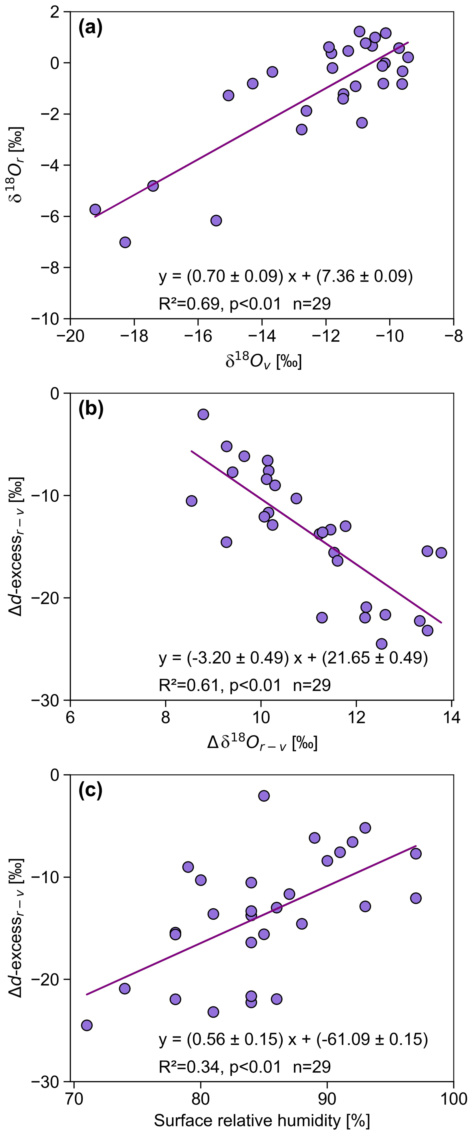
Figure 6 The correlations between (a) δ¹⁸O of rain (δ¹⁸O_r) and δ¹⁸O of vapour (δ¹⁸O_v) at the ground level, (b) the difference in d-excess of rain and vapour (Δd-excess_r − v) and δ¹⁸O (Δδ¹⁸O_r − v) showing that the rain value is lower in d-excess but higher in δ¹⁸O. (c) Difference in the d-excess of rain and vapour (Δd-excess_r − v) plotted against surface RH showing low correlation.

As raindrops evaporate, part of the newly formed vapour may get down-drafted to lower levels; the rain and vapour phases at the ground level would then exhibit opposite changes because the generated vapour is lower in δ¹⁸O but higher in d-excess compared to the rain. This happens when the evaporative contribution is large. However, in the case of tropical precipitation, the fractional addition from rain evaporation is small because the ambient vapour is a large reservoir. It has been shown in several earlier studies that the total rain constitutes only a few percent of the overhead vapour mass (Pathak et al., 2014; Rahul et al., 2016). Earlier studies have also shown that vapour d-excess values do not exhibit any systematic change in central or southern WG stations, but their rain δ¹⁸O values exhibit gradual depletion (1 ‰ to −10 ‰) in the latter part of the monsoon (Lekshmy et al., 2018; Rahul et al., 2016). The negative correlation found in this study, albeit minor, suggests that the ground-level vapour gets a significant contribution from drop evaporation. How can moisture generated by drop evaporation during raindrop descent contribute to the ground-level vapour? This is possible when there is a strong downdraft associated with intense monsoon rains (Risi et al., 2023). In a modelling study, Mandke et al. (1999) pointed out that deep convective cloud systems contain both upward and downward components. The downward motion is driven by evaporation of the falling drops and dragging of the ambient air and vapour by big droplets. This downdraft brings moisture down from above and increases the vapour d-excess at the ground (Risi et al., 2010; Kurita, 2013; Aemisegger et al., 2015).

The existence of drop evaporation is further supported by a relation between Δd-excess_r − v and surface RH (R² = 0.31; Fig. 6c). The difference between rain and vapour isotopes is higher (more negative) in lower RH and less in higher RH (Stewart, 1975). A similar analysis (Xing et al., 2023) in China also found that the change in isotopic composition is large when RH is less than 60 %.

Falling raindrops and the vapour in the atmospheric column constitute an interacting two-phase system. Below the cloud base, the water molecules are constantly exchanged between these two phases depending on the ambient RH and T. The difference between isotopes (δD_v and d-excess_v) of vapour in equilibrium with raindrops and the observed surface vapour (Δδ and Δd, respectively) is a useful signature of departure from equilibrium exchange. Graf et al. (2019) demonstrated how the Δδ − Δd plot can be used to decipher the effect of sub-cloud processes, such as evaporation and equilibration, which influence the rain isotopes. The time series of Δδ values (Fig. 7a) for the Pune rain samples shows that the values varied between −15 ‰ and 21 ‰. For Δd, the time series shows negative values in all cases (ranging from −2 ‰ to −24 ‰). The close-to-equilibrium samples correspond mostly to the high-humidity periods in July (Fig. 7b). Fifteen samples show the influence of below-cloud evaporation with positive Δδ values and associated strongly negative Δd values (up to −20 ‰).

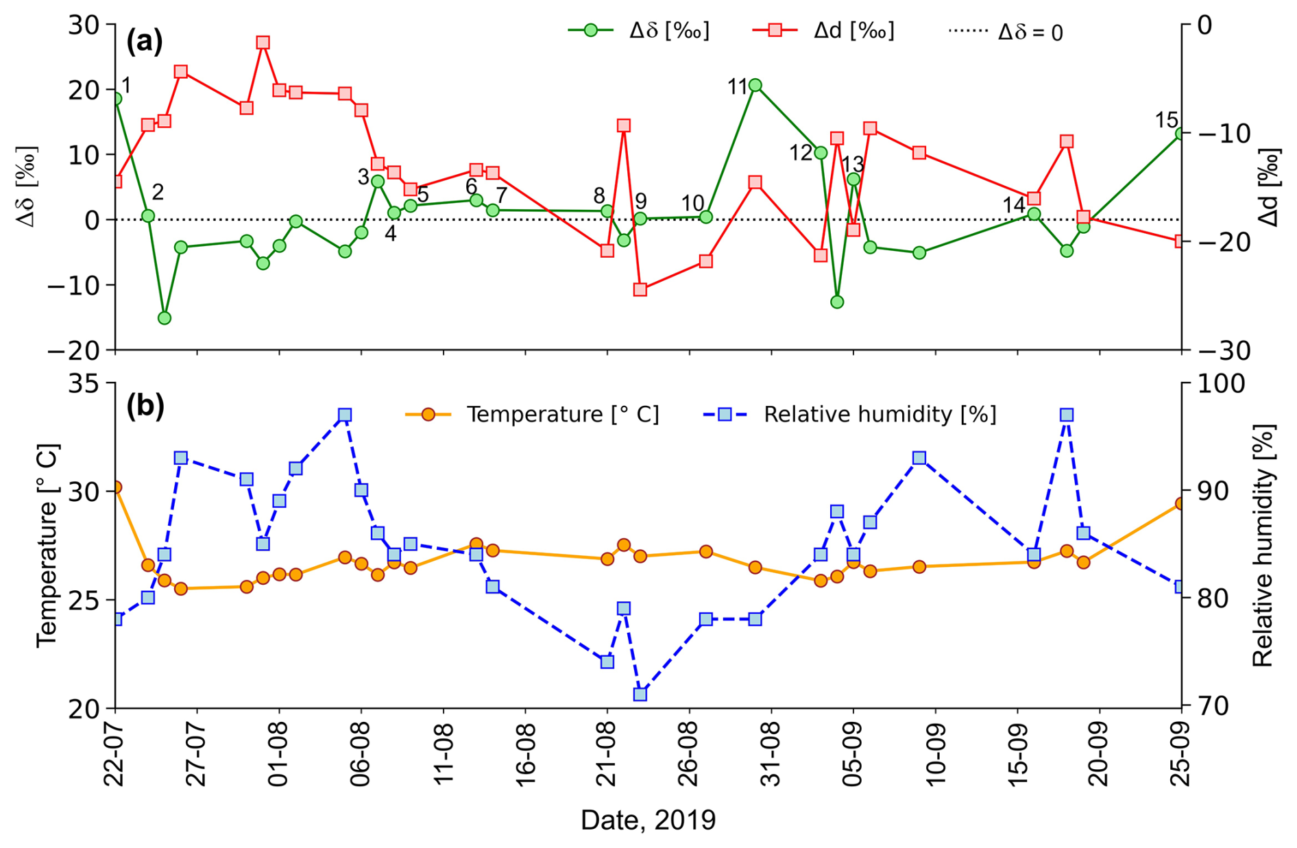
Figure 7 (a) Time series of Δδ and Δd of the rain samples collected during 2019 monsoon (July to September) in Pune. Δδ and Δd values (total points = 29) denote rain-equilibrated vapour isotope minus the surface vapour isotope. The blue dotted line indicates Δδ = 0. Data points with Δδ > 0 are marked with numbers 1–15. (b) Time series of daily average surface T and RH recorded at the IMD observatory at Pune.

A Δδ − Δd scatter plot (Fig. 8) shows that none of the rain samples is in equilibrium with the corresponding ground-level vapour. If the equilibrium pertained, the corresponding point would plot at the origin. Fifteen points fall in the lower right quadrant of the diagram (positive Δδ and negative Δd values), where the raindrop evaporation is relatively more significant. The rainfall amount for these samples was low (less than 5 mm d⁻¹), consistent with a substantial evaporation effect. Fourteen samples have both negative Δδ and Δd values (located in the lower left quadrant), indicating incomplete equilibration with near-surface vapour. The crucial driving factors for below-cloud processes seem to be the size of raindrops related to the intensity of precipitation. This is because raindrops with larger diameters correspond to increased intensity and have shorter residence times in the atmospheric column. As a result, they experience reduced evaporation during descent. It is to be noted that the drop diameter in this study was not measured by a disdrometer directly. They were estimated from the rain rate using the Marshall–Palmer relationship. Therefore, larger rain rates will always translate to larger droplet sizes. This physical relationship is thought to be a result of increased collision-coalescence during higher rainfall intensity (Law et al., 2021).

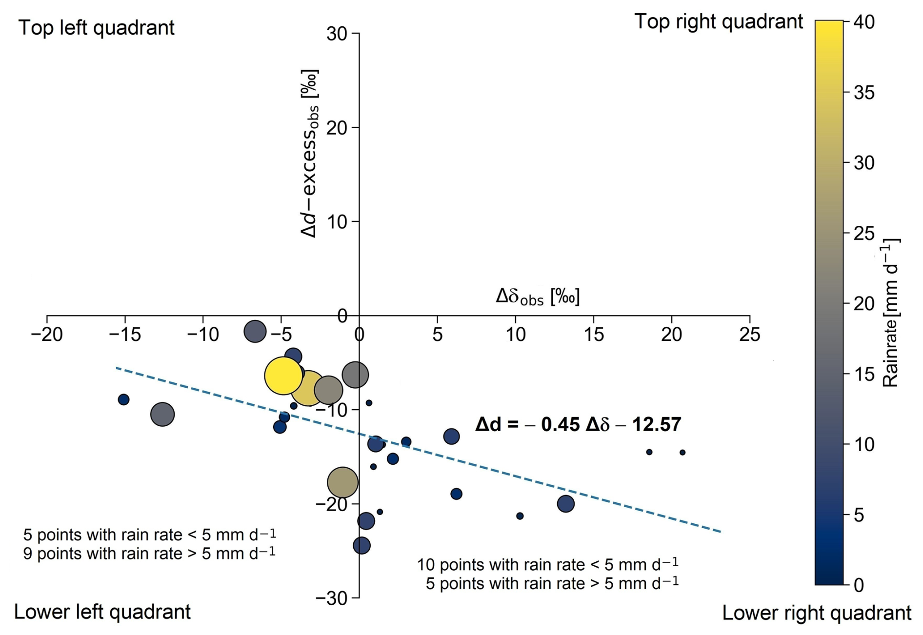
Figure 8 The Δδ − Δd cross plot of the sample isotope values along with the corresponding rain rates indicated by colour of the points. The size of the sample circles indicates drop size determined by the rain rate (scale on right) following the Marshall–Palmer formula. The line shows the best fit to the data points with a slope of −0.45.

Distribution of points in the Δδ − Δd plot (Fig. 8) shows that 10 samples with < 5 mm d⁻¹ rain rate fall in the lower right quadrant compared to 5 samples in the left quadrant. This suggests that drop evaporation is a dominant process in low rainfall events (where smaller drop diameters dominate). In Fig. 8, the size and colour of the points denote drop size and rainfall, respectively. It is clear that larger drop size points with higher rainfall plot in the lower left quadrant. This suggests that for larger sizes, the memory of the isotopes is partly retained despite the sub-cloud evaporation. Twenty-nine samples are nearly equally distributed in the two quadrants, suggesting an equal number of equilibration-dominant and evaporation-dominant rain events. It is to be noted that deep convective rains during the monsoon exhibit significantly higher mass-weighted diameter compared to shallow convective rains or stratiform rains (Kumar et al., 2025). The five big diameter points in the lower left quadrant correspond to cases of deep convection.

The regression line in the Δδ − Δd cross plot (Fig. 8) has a slope of −0.45 based on Bootstrap analysis (see Sect. S13). In contrast, Graf et al. (2019) obtained a smaller value of −0.30 for their study area, Zurich, Switzerland. The difference is intriguing and merits a discussion. Their study was based on short-time intra-event samples (covering about 16 h and each rain sample being collected for 10 to 15 min) in a mid-latitude region, whereas Pune samples were 29 daily rain collections in a tropical region (covering a few months and each collected for 24 h). A set of complex processes operates to dictate the value of the slope, and Graf et al. (2019) pointed out that the slope could represent a balance between below-cloud evaporation and equilibration. They suggested that it would be insightful to explore the slope for other climatic regions, hinting that the slope will help assess the evaporation. A quantitative estimate of the evaporation fraction can be obtained from BCIM by using the mass loss parameter in the output (see Sect. 4.3).

At higher humidity, the evaporation is lower, the change of Δd is smaller, and this leads to a lower slope. Conversely, when the temperature is higher, the slope is higher due to higher evaporation. The value of the slope is determined by a differential effect in evaporative fractionation. Evaporation decreases d_r, and increases δD_r, but the magnitudes of these changes (negative for d_r and positive for δD_r) are not the same. Fractionation values (involving equilibrium and kinetic effects) show that the change in δD_r is larger compared to that in d-excess (about 30 % of the δD_r change, considering absolute values). This is because in evaporation, the kinetic fractionation occurs along with equilibrium fractionation, and the former has more influence on δD compared to δ¹⁸O. If evaporation is higher (due to higher T and lower RH), the deviation of the predicted rain isotope values from those predicted by the equilibrium fractionation alone will be more, and the slope will be higher. In the frontal systems of Switzerland, the T was about 12 °C and RH about 80 % (Graf et al., 2019), whereas in Pune, the T was about 25 °C and RH about 85 %. Even though the RH was nearly similar, the T was much higher in Pune, which resulted in a higher slope for Pune (see next section).

4.3 Estimate of raindrop evaporation

As per the simulation of BCIM, the mass of the drop reduces as it falls. The ratio of final mass to the initial mass ($m/m_{\mathrm{o}}$) can then be used to estimate the fractional mass loss suffered by the drop on its way down. The difference (1 − $m/m_{\mathrm{o}}$) represents the effective rain evaporation. With this definition, a time series of evaporation values (Fig. 9a) shows variation from 4 % to 61 %. The average evaporation is 23 % if we consider all 29 values. But there are four large values 45 %, 47 %, 58 % and 61 %, all of which correspond to low rainfall or small drop diameter (Fig. 9d). If we exclude them, the average is 18 % (n = 25). As expected, drop evaporation is inversely related to relative humidity (Fig. 9b) and drop diameter (Fig. 9d) but directly proportional to the temperature (Fig. 9c). The relative importance of the three determining factors, namely, RH, T and drop diameter, is seen through the multiple regression equation of evaporation fraction. Here, we should use normalized multiple regression because simple (or unnormalized) multiple regression uses variables in their original units, while normalized multiple regression transforms all features onto a similar scale, allowing for direct comparison of feature importance. The normalized evaporation fraction as a function of normalized values of RH, T and D shows that (1) D is the major determinant and (2) T plays an important role, nearly as much as RH, for evaporation.

$$\begin{array}{}\text{(2)}& \begin{array}{rl}& \text{Normalized Evaporation Fraction}\\ & =-{\mathrm{0.329}}^{*}\text{RH}+{\mathrm{0.370}}^{*}T-{\mathrm{0.665}}^{*}\text{Diameter}\end{array}\end{array}$$

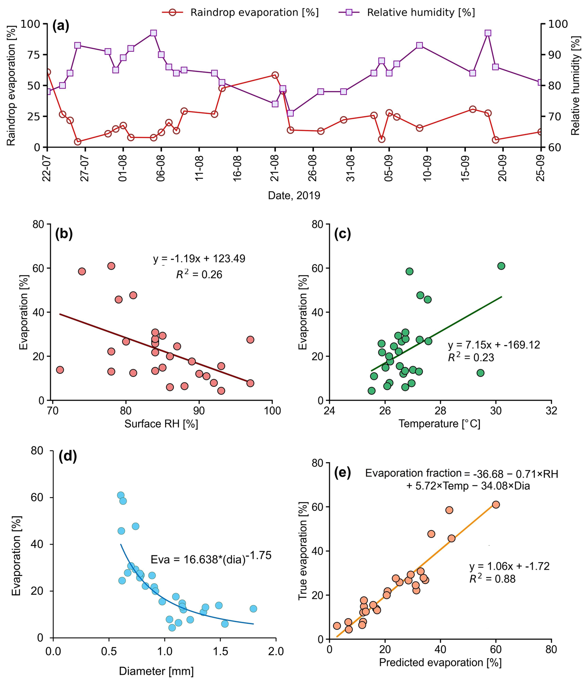
Figure 9 (a) Time series of raindrop evaporation using Run-3 of BCIM simulation and surface relative humidity. The regression between raindrop evaporation fraction with (b) RH, (c) temperature, and (d) drop diameter. (e) Multiple regression analysis yields the equation shown in the inset. The regression equation explains nearly 88 % of the variance in the evaporation.

For the larger values of temperatures, we expect more evaporation; this leads to the higher slope value of −0.45 (in the Δδ − Δd cross plot in Fig. 8) for Pune compared to −0.30 for Zurich, as noted in the previous section.

The evaporation was particularly high (61 % and 59 %) on 22 July and 21 August due to combined effect of low RH (78 % and 74 %), and high T (30 and 27  °C) and small D (Fig. 9a). On average, the evaporation fractions are moderately high (23 ± 16) % which is consistent with the observed anticorrelation between d_r and δ¹⁸O_r of rain samples (Fig. 4b).

4.4 The uncertainty in the evaporation fraction

Among the controlling factors for evaporation, the temperature does not vary much (26.8 ± 1.0 °C) or about 4 %, while for RH, the variation is slightly larger (85 ± 6 %) or 7 %. The diameter variation, on the contrary, is much higher, about 30 % (1.0 ± 0.3 mm) and has a higher impact on the evaporation. The net uncertainty in the evaporation fraction due to combined uncertainties in RH, T and D can be determined by a simple multiple regression equation (using unnormalized variables) as given below. The Evaporation Fraction (EF) was regressed with RH (in %), T (in °C) and D (in mm) and yields:

$$\begin{array}{}\text{(3)}& \mathrm{\text{Evap. Fraction}}=-\mathrm{36.68}-{\mathrm{0.71}}^{*}\text{RH}+{\mathrm{5.72}}^{*}T-{\mathrm{34.08}}^{*}D\end{array}$$

Equation (3) can be used to estimate the error in drop evaporation, knowing the uncertainties in RH, T and D and using the partial regression coefficients as partial derivatives. Using the standard quadratic formula for error (Farrance and Frenkel, 2012), we write:

$$\begin{array}{}\text{(4)}& \begin{array}{rl}\mathit{\sigma }(\text{EF}{)}^{\mathrm{2}}& ={{\left(\partial \text{EF}/\partial \text{RH}\right)}^{\mathrm{2}}}^{*}(\text{RH}{)}^{\mathrm{2}}+{{\left(\partial \text{EF}/\partial T\right)}^{\mathrm{2}}}^{*}(T{)}^{\mathrm{2}}\\ & +{{\left(\partial \text{EF}/\partial D\right)}^{\mathrm{2}}}^{*}(D{)}^{\mathrm{2}}\end{array}\end{array}$$

where σ denotes the uncertainties in EF, RH, T and D, and the quantities in brackets express the partial derivative of EF with respect to the variable (see Eq. 3). The uncertainties associated with RH (see Sect. S14; Fig. S15), T and D are discussed in Sect. S10. Adding these three errors by the above quadratic formula, we obtain the error in the evaporation fraction for 29 d, which varies from 7.4 % to 13.8 % (for EF values from about 4 % to 61 %). The average for 29 d is ±8.9 %, which is taken as the overall error in the evaporation estimate.

4.5 Evaporation and rainfall relation

Evaporation fraction plotted as a function of rainfall (Fig. 10) shows a power law. For a smaller rainfall range (less than 5 mm d⁻¹), evaporation affects the rainfall significantly. The reason is that smaller rainfall is usually associated with smaller drops, which are very sensitive to evaporation, resulting in a power law. If the EF increases by 10 % (say from 15 % to 25 %), the rainfall reduces by about 4 mm d⁻¹ (from 5 to 1 mm d⁻¹).

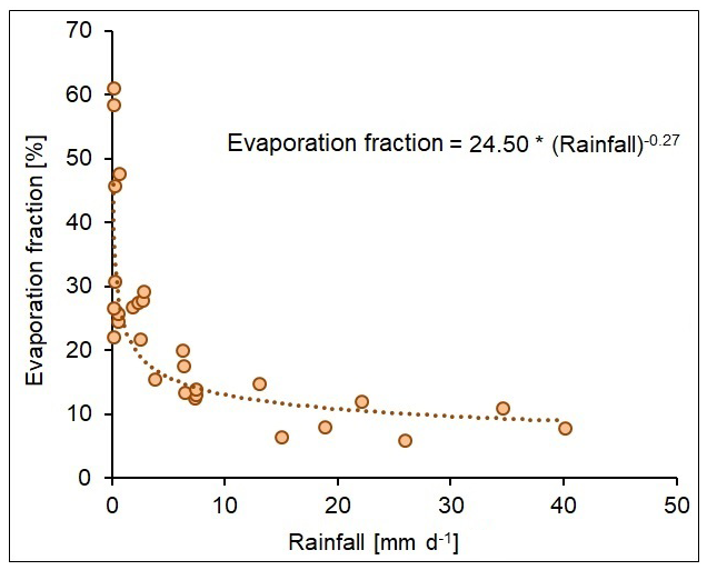
Figure 10 A scatter plot shows the relationship between the estimated raindrop evaporation and rainfall in Pune. The brown dotted line indicates the best-fit power law. Higher rainfall implies drops of bigger size and hence lower evaporation fraction.

It is instructive to compare our results to the evaporation estimates obtained in similar studies carried out in other climatic regimes. Using a steady state one-dimensional model of rain in the North Atlantic Trade Wind region (Barbados), Sarkar et al. (2023) found a high value of 63 % (63 ± 23 %) for raindrop evaporation (using radar reflectivity data of rain evaporation flux), which is three times more than our average value of 23 % (23 ± 16 %). The reason for the large difference in Pune evaporation from Barbados is possibly due to a large difference in drop diameter and RH. A comparison reveals that in Barbados, the drop diameter was much smaller (from 0.1 to 0.6 mm) in comparison to ours (from 0.61 to 1.80 mm). The Barbados drops were so small that in some cases (for example, smaller than 0.3 mm on 4 February 2020) they evaporated completely (evaporation ∼ 100 %) during descent. In addition, in their sampling region, the RH was lower, ranging from 65 % to 80 %, compared to ours (74 % to 97 %). A smaller drop diameter and lower RH lead to higher raindrop evaporation. In contrast, only four high evaporation days (more than 45 %) occurred in Pune out of 29 sampling days. We also note that their drop diameters varied over a wider range, leading to a larger variability compared to our study.

In a similar study as here, rain and vapour isotopes were measured in a cold-front passage over Zurich during 19–25 July 2011, and the data were interpreted by an isotope-enabled regional weather prediction model COSMOiso (Aemisegger et al., 2015). The authors showed that by switching off the raindrop evaporation, the rainfall increased by about 75 % because the cooling induced by evaporation causes diminished convective activity. The estimated average evaporation in their study was about 40 %. This value is nearly twice our average value. The reason is probably a smaller drop diameter and lower RH and the authors write: “weak rainfall intensities (small droplets and thus lower falling velocities), and possibly lower relative humidity in the air column could have contributed to the evaporative enrichment of precipitation”.

4.6 Limitations and uncertainty of the derived parameters

The present study using the BCIM applied to the Pune region is associated with the following limitations:

• 1.

  We used TES satellite data averaged over 2005–2009 to guide our choice of vapour isotope profiles, but the year of analysis was 2019. In this matter, there is no way to ascertain the degree of deviation of the true profiles from the adopted ones in Run-3.

• 2.

  There are limitations on the use of RH and T from radiosonde. However, the mean radiosonde data for Pune are expected to be reasonable if we can show that the difference between the two consecutive measurements is not large. Radiosondes are launched at 00 and 12Z and are generally not carried out when there is rain. We determined that the two soundings taken on the same day are similar to within 8 % RH and 1 °C on most days (Fig. S15). Analysis of radiosonde daily variability can be found in Sect. S14. We also show through sensitivity analyses and multiple regression analyses that the effects of the daily scale variation in RH and T on model rain isotope values and evaporation fractions are not significant. We demonstrate further that the RH and T data from the radiosonde are more reliable than the same obtained from any satellite datasets.

• 3.

  The δ¹⁸O_v profiles were adopted based on the δD_v and δ¹⁸O_v profiles obtained from the LMDZ model. Run-3 uses radiosonde data for the thermodynamic profiles, δD_v from satellite data of 2005–2009, and δ¹⁸O_v from the d_v of the LMDZ extrapolated to the observed vapour measurement at the ground. We realize that there are major concerns with these inputs coming from different data products that have different spatial/temporal scales and measurement principles. But we note that whenever any atmospheric model is initialized, the input parameters from various sources are used, which may have different spatial and temporal resolutions and measurement principles. Moreover, datasets from various sources are also utilized in atmospheric models across different parametrization schemes and nudging. In support of the adopted isotope tuning, we note that nudging is a well-known technique where the model values are adjusted to accord with the observed values. For example, Graf et al. (2019) used point-based radiosonde RH and T observations, as well as isotope outputs from a limited-area model (Pfahl et al., 2012; Villiger et al., 2023), with a km-scale resolution. These two datasets have different scales and measurement principles. Guided by their argument, we have taken the average radiosonde profiles of each sampling day as our choice and adjusted the lowermost parts to match the measured RH and T values at the ground taken from the IMD.

• 4.

  The isotope profiles were constructed initially using ground observations as boundary values. However, this resulted in a mismatch with the observed values in Run-2, and we had to tune to lower δD_v values and higher δ¹⁸O_v values (and consequently lower d_v values) to achieve good agreement. It should be mentioned here that Risi et al. (2023) discussed a similar idea in their study of water isotopes in tropical squall lines; they indicated that convective downdrafts can introduce depleted vapour produced by rain re-evaporation in the boundary layer. Another limitation in this study is that the vapour samples were collected for a duration of about a few hours, which did not coincide exactly with the 24-h rain collection period.

• 5.

  The raindrop formation height was assumed to be the CLWC peak level for all rainy days, and the drops were all introduced at that level. However, it is well known that raindrops do not all form at the same height, even on a single day. With the single height assumption for drop introduction, we are neglecting alterations in isotope ratios produced inside the cloud by various microphysical processes.

• 6.

  Although some studies pointed out that collision-coalescence is an important warm rain process that occurs in the WG regions of India (Konwar et al., 2014), we did not include it in the model. Since the BCIM follows the evolution of a single droplet, there is no opportunity to introduce collision coalescence, and we have to rely on the input droplet diameter being representative of droplet sizes that would occur through collision-coalescence processes. In theory, this is all built into the Marshall–Palmer relationship.

• 7.

  The uncertainty values for δD_r is 3.5 ‰, for d_r it is 1.7 ‰, and for drop evaporation it is 8.9 %. Several assumptions are required to calculate the uncertainties in these parameters (details are given in Sects. S10 and S11), and some of them (like the linear dependence assumption in multiple regression) may be open to questions.

4.7 Impact of evaporation on rainfall and heat budget

Evaporation of raindrops during the ISM has been postulated earlier in several theoretical models, but this study provides, for the first time, a quantitative estimate of rain evaporation on a day-to-day basis in the monsoon season using combined rain and vapour isotope data in a BCIM. We found that about 23 % raindrop evaporation occurred in the 2019 monsoon season in the highly humid Pune region. The average seasonal rainfall in Pune is about 55 cm (during monsoon), and if ∼ 23 % of this is evaporated, it would mean considerable cooling of the boundary layer, leading to localized downdrafts, formation of cold pools, and changes in atmospheric stability. Cooling can also hinder efficient formation of convection (Hwong and Muller, 2024) and can have a large effect on the precipitation patterns in the tropics (Bacmeister et al., 2006; Sarkar et al., 2023). Given the large share of precipitation recycling found in this study for Pune, the question arises as to how large the precipitation recycling is at regional or continental scales. We need to have a comprehensive program for carrying out such analysis, aided with appropriate BCIM input parameters, to understand the evaporation of raindrops over various climatic subdivisions in India. Moreover, high-frequency observations of vapour and rain isotopes would be useful to quantify this fraction during various convective events associated with low-pressure systems during the monsoon. A quantitative estimate of raindrop evaporation would be highly useful for modelling the energy and moisture budgets during the monsoon season.

5 Conclusions

This study reveals substantial temporal variability in atmospheric vapour isotopes in Pune during the 2019 monsoon, with δ¹⁸O_v ranging from −19.2 ‰ to −9.4 ‰ and δD_v from −123.7 ‰ to −63.4 ‰. Rain isotopes show comparatively smaller variability (δ¹⁸O_r: −7.5 ‰ to 1.2 ‰; δD_r: −58.9 ‰ to 11.8 ‰). Four events of markedly depleted rain and vapour isotopes were identified, coinciding with negative OLR anomalies and high rainfall indicative of strong convection and the effect of Rayleigh condensation. These events likely reflect the uplift of moist air parcels to higher altitudes (∼ 5.5 km) and condensation to droplets during ascent following Rayleigh distillation.

Vapour isotope data show a distinct seasonal trend, with increasing vapour d_v and decreasing δ¹⁸O_v after mid-August, particularly in September. The strong anticorrelation between vapour δ¹⁸O_v and d_v at the ground suggests increasing contributions from evaporative sources over time. Downdrafted vapour with potential contribution from raindrop evaporation possibly constitutes one such source. Δδ − Δd analysis further confirms the importance of sub-cloud evaporation, with ∼ 50 % of data points falling in the evaporation-dominated quadrant. The derived slope (−0.45) indicates stronger evaporation compared to mid-latitude systems, consistent with higher temperatures (∼ 25 °C) in Pune, enhancing kinetic fractionation effects.

To quantify the sub-cloud processes altering the rain isotope values, we used the BCIM. Upon reasonable tuning of the input parameters, we obtained good agreement between the observed and model rain isotope values at the ground level. Using the model, raindrop evaporation is quantified on a daily scale, revealing an average mass loss of ∼ 23 % (range: 4 %–61 %) in the sub-cloud layer. Excluding the extreme cases, evaporation averages 18 ± 8 %, which introduces substantial modification of isotopes of raindrops during their fall. Raindrop evaporation can reduce the rainfall substantially, especially during low rain (less than 10 mm d⁻¹). In addition, the evaporation can cool the boundary layer leading to localized downdrafts and hindering formation of convection.

The isotope based BCIM used for estimating raindrop evaporation fraction in this study has many limitations which include constructing vapour isotope profile with TES data available for a different period, using values of input parameters (in Run-2 and Run-3) from multiple data sources having different spatiotemporal resolution, a mismatch in rain and vapour collection periods, assuming the CLWC peak height as the drop formation altitude, and neglecting collision-coalescence. These limitations and their associated uncertainties are explicitly discussed in Sect. 4.6.

Our current findings pave the way for several avenues of future research. Future studies should prioritize continuous, high-resolution measurements of atmospheric water vapor and rain isotopes to quantify event-based raindrop evaporation. Additionally, deploying an isotope-enabled limited-area model over the study region will reduce uncertainties in model-derived vapor isotope profiles, yielding more precise estimates of the evaporation fraction. Long-term observations spanning multiple monsoon seasons across a broader network in the Western Ghats will help map the spatial and temporal variability of sub-cloud evaporation. Finally, further work is necessary to determine the influence of these processes on regional moisture recycling, monsoon energy budgets, groundwater recharge, and projected changes in monsoon precipitation under future climate scenarios.