Causal inference for quantifying chemical–dynamical pathways controlling tropical middle stratospheric ozone variability

Understanding the chemical–dynamical interactions controlling ozone (O₃) variability in the tropical middle stratosphere is essential for interpreting short-term trends and their sensitivity to dynamical fluctuations. This study applies a process-oriented causal inference framework that combines causal discovery and causal effect estimation. This approach integrates qualitative physical knowledge through a causal graph applied to satellite observations and a chemistry-transport model (CTM) simulation, using monthly data for the period 2004–2021. Causal inference robustly identifies a dominant chemical–dynamical pathway, in which variability in residual vertical velocity (w^*) modulates nitrous oxide (N₂O), subsequently affecting nitrogen dioxide (NO₂) and ultimately O₃. Estimates of direct causal effect capture that O₃ variability is dominated by this indirect NO₂-mediated pathway, while the direct influence of w^* on O₃ is weak. The total causal effect (direct and mediated) peaks at a lag of approximately two-three months, indicating the cumulative impact of persistent, vertically coupled w^* anomalies associated with the QBO. Regime-oriented analysis applied to the observations reveals that the chemical links (N₂O–NO₂ and NO₂–O₃) strengthen during westerly QBO shear compared to easterly shear.

Our study highlights the pivotal role that causal inference can play in disentangling complex chemical-dynamical influences on O₃, complementing traditional statistical methods. This approach lays the foundation for broader applications in stratospheric chemistry, where the understanding of various feedback pathways remains uncertain. By discovering and quantifying causal links, this methodology can be adapted to address open questions with environmental and societal relevance. Integrating causal reasoning into data-driven science can enhance process understanding and also strengthen the synergy between machine learning and statistical methods in Earth and environmental sciences.

1 Introduction

Stratospheric ozone (O₃) is essential for protecting life on Earth by absorbing most of the harmful solar ultraviolet (UV-B) radiation (280–315 nm). The tropical (10° S–10° N) middle stratosphere (∼10 hPa) is a key region for the photochemical formation of O₃ (Chapman, 1930). A balance between photochemical production and loss, together with dynamical transport, determines the overall abundance of stratospheric O₃ (Match et al., 2025). Its global distribution and inter-annual changes are mainly determined by dynamical and chemical processes in conjunction with their superimposed variability of different origins and periodicity, such as Brewer–Dobson circulation (BDC), El Niño–Southern Oscillation (ENSO), Quasi-Biennial Oscillation (QBO), concentrations of greenhouse gases (GHGs) and Ozone Depleting Substances (ODSs). Reduction in stratospheric O₃ concentrations allows more UV radiation to reach the Earth's surface, resulting in harmful effects, including damage to plant life and crops, disruption of aquatic ecosystems, and increased risks of skin cancer, cataracts, immune suppression, and erythema in humans (WMO, 2022; Zerefos et al., 2023). To mitigate these harmful effects, actions taken under the Montreal Protocol and its Amendments and Adjustments have significantly reduced emissions and atmospheric abundances of ODSs, contributing to the recovery of the stratospheric O₃ layer.

Apparent changes in tropical middle stratospheric O₃ can vary substantially depending on the length and timing of the analyzed period. For example, in the early 2000s, several studies reported statistically significant O₃ decline in this region using a variety of datasets and methodologies (Kyrölä et al., 2013; Eckert et al., 2014; Gebhardt et al., 2014; Nedoluha et al., 2015; Galytska et al., 2019; Arosio et al., 2019; Iglesias-Suarez et al., 2021). Subsequent analyses showed that the slight differences in the tropical O₃ trends across different data sources arise from small shifts in the analyzed time period, largely due to endpoint anomalies influenced by the curvature of long-term O₃ variability and unaccounted fluctuations in the record (Petropavlovskikh et al., 2019; Sofieva et al., 2021). Recent assessments show that the magnitude of O₃ trends in the tropical middle stratosphere since the early 2000s is highly uncertain (−2 % to 0 % per decade, WMO, 2022) with multiple studies finding no statistically significant or robust long-term trend across different datasets and time periods (Petropavlovskikh et al., 2019; Steinbrecht et al., 2017; Godin-Beekmann et al., 2022; Arosio et al., 2024). In addition, Szeląg et al. (2020) highlighted a strong seasonal dependence in tropical middle stratospheric O₃ trends during 2000–2018, with a significant increase in spring (2 %–3 % per decade) and a non-significant decrease in autumn (−1 % to −2 % per decade), resulting in non-significant trends, consistent with Galytska et al. (2019); Li et al. (2023). However, the absence of a persistent long-term trend in recent analyses does not rule out future changes of O₃ in the tropical middle stratosphere. Similarly, negative trends observed in the early 2000s could recur if comparable dynamical–chemical conditions arise. In this context, understanding the mechanisms governing interannual O₃ variability becomes particularly important, as such variability can substantially influence trends derived from a limited observational dataset.

While previously discussed O₃ trends motivate this study, our objective is to quantify the mechanisms that control O₃ variability on monthly timescales and thus, that can modulate trends over limited time periods. The sensitivity of O₃ trends in the tropical middle stratosphere to the analyzed period highlights the dominant role of chemical–dynamical variability in this region. In this context, Galytska et al. (2019) showed that the O₃ decline observed in the early 2000s was dynamically controlled and linked to increases in nitrogen dioxide (NO₂). The elevated NO₂ levels enhanced O₃ loss through the catalytic NO_x (NO${}_x=\mathrm{NO}+{\mathrm{NO}}_{\mathrm{2}}$) cycle, dominant in the middle stratosphere (Portmann et al., 2012). The increase in NO₂, also confirmed by Dubé et al. (2020), resulted from the prolonged residence time of its primary source, nitrous oxide (N₂O). Since N₂O is a long-lived species (Portmann et al., 2012; Chipperfield et al., 2014), the changes in its abundance reflect variations in tropical upwelling within the BDC, therefore, they are directly affected by changes in stratospheric transport (Iglesias-Suarez et al., 2021). Prather et al. (2023) showed that during 2005–2021, N₂O increased in the tropical middle stratosphere more than expected from the rate of tropospheric increases. This implies a more vigorous BDC, leading to a shorter lifetime. Minganti et al. (2020) evaluated the climatological impact of the stratospheric BDC on N₂O and reported that, in the tropical middle stratosphere, the interannual variability of vertical residual advection exhibits a significant spread, which reflects the influence of the major source of interannual variability in the equatorial stratosphere, i.e. the QBO on tropical upwelling (Abalos et al., 2015). Chipperfield and Gray (1992), and later Park et al. (2017) highlighted that the source gas N₂O and the reactive nitrogen species (NO_y) display coherent QBO signals within the tropical stratosphere. O₃ also exhibits a strong QBO signal, with the QBO directly influencing O₃ levels by altering the chemical reactions responsible for O₃ depletion, see also Chipperfield et al. (1994) and Ming et al. (2025). This oscillation modulates the rates of these reactions, leading to additional variations in O₃ concentration. It is also important to note that recent work by Hitchcock and Ming (2025) demonstrates that ozone can play a leading role in modulating the QBO, highlighting a two-way chemical–dynamical interaction, which is the subject of ongoing research and clarification (Orbe et al., 2026).

Therefore, to set the stage for our subsequent causal analysis of these chemical-dynamical feedback pathways on O₃ variability in the tropical middle stratosphere, Fig. 1 presents scatter plots of detrended monthly mean anomalies of (a) residual vertical velocity (w^*) versus N₂O, (b) N₂O versus NO₂, (c) NO₂ versus O₃, and (d) N₂O versus O₃ for observations and the TOMCAT CTM simulation for 2004–2021. Both observations and the TOMCAT CTM simulation exhibit similar correlations and slopes. The relationship between w^* and N₂O is moderately positive (panel a). The strong anti-correlations between N₂O and NO₂ (panel b) result from their opposing response to transport-driven variability, where, e.g. enhanced upwelling increases N₂O while reducing its chemical loss, which is crucial for NO₂ production (see further discussion in Sect. 4.1). The negative relationship between NO₂ and O₃ (panel c) is a result of NO₂ being the primary sink of O₃ in the middle stratosphere (Park et al., 2017). The positive relationship between N₂O and O₃ (panel d) reflects transport-controlled variability in N₂O, while O₃ is mainly controlled by photochemistry (Brasseur and Solomon, 2005); the observed correlation results from both tracers varying systematically with altitude in the tropical middle stratosphere.

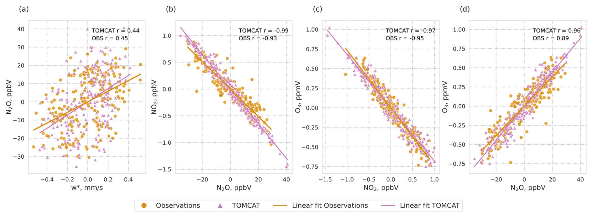
Figure 1 Scatter plots of detrended monthly mean anomalies in the tropical middle stratosphere for 2004–2021, from observations (circles) and the TOMCAT CTM simulation (triangles). Panels show (a) w^* versus N₂O, (b) N₂O versus NO₂, (c) NO₂ versus O₃, and (d) N₂O versus O₃. Solid lines indicate linear regressions for observations (orange) and TOMCAT (pink). The corresponding Pearson correlation coefficients (r) are shown in each panel.

While the key chemical reactions and dynamical processes governing tropical middle-stratospheric O₃ have been identified and can be simulated in chemistry-climate models (CCMs), previous research relies mostly on correlation and different types of regression analyses that do not explicitly distinguish between direct and mediated causal effects within a multivariate system. A causal inference framework proposed in this study represents the relationships between the selected variables as a directed acyclic graph (DAG), in which nodes correspond to physical quantities and edges represent causal influences. Therefore, the structure of the DAG is informed by established physical understanding and subsequently evaluated using causal inference methods applied to the data. Causal inference can then be used to estimate the targeted relationships under explicit assumptions. Applying such an approach to a well-understood chemical–dynamical system provides a reliable test of whether causal inference can recover known physical pathways and quantify their contributions in the analyzed system. To connect the discussion of stratospheric chemical–dynamical interactions with the causal inference framework used in this study, Appendix A provides a glossary that links key causal terms to their interpretation in a stratospheric context. For a broader overview of the terminology, the reader is referred to Camps-Valls et al. (2023) and Runge et al. (2023). It is important to highlight that to ensure statistical consistency, this study analyzes detrended anomalies rather than long-term trends. Therefore, the results describe variability-driven processes and should not be interpreted as a direct explanation of decadal O₃ trends caused by externally forced long-term changes in CO₂, N₂O emissions, or ODSs, but rather in the context of dynamical processes that are strongly influenced by the QBO.

2 Data sources

This study uses monthly data from satellite observations, reanalysis products, and a TOMCAT CTM simulation, focusing on four core variables, namely w^*, N₂O, NO₂, and O₃. We also use a measure of the QBO as an additional variable to examine how the relationships among the four core variables vary under different dynamical regimes. By selecting these variables, we focus the analysis on the interpretability of key chemical-dynamical processes that play a major role in controlling O₃ in the tropical middle stratosphere. We intentionally limit the number of variables to maintain a high level of interpretability of the causal graphs. We then compare the causal graphs from observations and the TOMCAT CTM simulation.

2.1 Observations

Since no single satellite instrument provides all the required variables with sufficient temporal and spatial resolution, we integrate data from multiple sources into this study. The following observational or reanalysis-based datasets were used:

• w^*: Derived Transformed Eulerian Mean (TEM) momentum terms (v0.1.1, Serva, 2022), based on European Centre for Medium-Range Weather Forecasts (ECMWF) ERA5 reanalysis (Hersbach et al., 2020) using diagnostics from Serva (2023); Serva et al. (2024);

• N₂O: Profiles from the Earth Observing System (EOS) Microwave Limb Sounder (MLS, v5.01) instrument on NASA's Aura satellite, which offer a vertical resolution of 5–8 km and a horizontal along-track resolution of 165–265 km (Lambert et al., 2020);

• NO₂: Profiles retrieved from limb-scattered sunlight observations on the OSIRIS instrument aboard the Swedish Odin satellite (Murtagh et al., 2002; Llewellyn et al., 2004). OSIRIS NO₂ v7.3 is retrieved via spectral fitting in the 435–477 nm range from 10.5 to 39.5 km with a 2–3 km vertical resolution in most of the stratosphere (Dubé et al., 2022). Due to the pronounced diurnal cycle of NO₂ (Galytska, 2019; Dubé et al., 2020) the photochemical correction from Dubé et al. (2020) was applied to standardize all measurements to a reference time of 12:00 p.m. local solar time;

• O₃: OSIRIS O₃ v7.3 (Bognar et al., 2022), an improved version of the v5.10 product with corrected long-term drift by accounting for systematic errors in the instrument limb-pointing (Bourassa et al., 2018);

• QBO: equatorial zonal mean zonal wind taken from the Institute of Meteorology and Climate Research, Karlsruhe Institute of Technology, see Kerzenmacher and Braesicke (2026).

In the following, the combination of these datasets is collectively referred to as “observations”.

2.2 TOMCAT Chemical Transport Model

TOMCAT is a three-dimensional off-line CTM (Chipperfield, 2006), driven here by winds and temperatures from the ERA5 reanalysis (Hersbach et al., 2020). Given prescribed atmospheric transport and temperature fields, TOMCAT calculates the distributions of chemical species in the troposphere and stratosphere. A stratospheric full-chemistry simulation, including all of the NO_y chemistry discussed in this paper, was run at a horizontal resolution of 2.8° × 2.8° with approximately 1.5 km vertical resolution in the stratosphere (Chrysanthou et al., 2025). The model uses time varying sulfate aerosol surface area density Dhomse et al. (2015), solar fluxes (Dhomse et al., 2016), and lower boundary concentrations of GHGs and ODSs (WMO, 2022), recommended for CMIP6 simulations. We used the monthly average output in our analysis. The TOMCAT CTM simulation was chosen for its ability to provide a continuous time series without spatial or temporal gaps, making it ideal for robust comparison with the observational datasets.

2.3 Data preprocessing

Monthly anomalies of w^*, N₂O, NO₂, and O₃ in the tropical (10° S–10° N) middle (10 hPa) stratosphere were calculated from observations and the TOMCAT CTM simulation relative to the climatological mean over August 2004–December 2021. The analysis begins in August 2004, due to the availability of MLS N₂O observations. However, for simplicity, we refer to the period as 2004–2021. To maintain a robust comparison against temporal sampling discrepancies, TOMCAT CTM data were masked to align with observations, omitting any dates with missing observational data. For causal inference, all time series were standardized. Since the application of causality requires the stationarity of the time series (see Sect. 3.1), we remove the linear trends from all analyzed time series. For more details about preprocessed timeseries from observations and the TOMCAT CTM simulation and their further comparison, see Appendix B.

3 Methods

3.1 Causal inference

We apply the latent Peter-Clark momentary conditional independence (LPCMCI) algorithm (Gerhardus and Runge, 2020), which is an extension of the PCMCI+ algorithm specifically designed to deal with latent (i.e. unobserved) variables (Runge et al., 2019b; Runge, 2020). LPCMCI employs ideas from the Fast Causal Inference (FCI) algorithm to learn not only directed causal relationships but also infer the presence of latent confounders (Spirtes, 1995). LPCMCI benefits from the same ideas underlying PCMCI+ by increasing the effect size of conditional independence (CI) tests through including causal parents in conditioning sets. The LPCMCI method seeks to learn a Directed Partially Ancestral Graph (DPAG), which captures the causal relationships among the observed variables. In contrast to Maximal Ancestral Graphs (MAGs) that contain directed arrows (→) and bidirected edges (in other words, double-headed arrows ↔), PAGs can include additional edge types. These edges, drawn as $\circ \to$ and/or $\circ \text{-}\circ$, indicate the presence of hidden variables or uncertainty about the exact causal direction.

To understand the causal structure of the underlying complex dynamical system, the observed time series ${\mathit{X}}_{\mathit{t}}=(X_t^{\mathrm{1}},\mathrm{\dots },X_t^N)$, where N stands for the different variables represented by time series, is assumed to follow the following causal process:

$$X_t^j=f_j\left(\mathcal{P}\left(X_t^j\right),{\mathit{\eta }}_t^j\right),$$

where f_j is a measurable function that depends on all its inputs, ${\mathit{\eta }}_t^j$ represents dynamical noise (independent across $t^{\prime }\ne t$). Here, $\mathcal{P}\left(X_t^j\right)\subset {\mathit{X}}_{t+\mathrm{1}}^{-}=({\mathit{X}}_t,{\mathit{X}}_{t-\mathrm{1}},\mathrm{\dots })\setminus \mathit{\left\{}{X}_t^j\mathit{\right\}}$ denotes the set of parent variables of $X_t^j$ since the value of $X_t^j$ is determined from the variables in $\mathcal{P}\left(X_t^j\right)$ and the dynamical noise ${\mathit{\eta }}_t^j$. Bidirected links between $X_t^i$ and $X_t^j$ in this model imply that the associated noise terms ${\mathit{\eta }}_t^i$ and ${\mathit{\eta }}_t^j$ are dependent through unobserved confounding. We assume causal stationarity, meaning $X_{t-\mathit{\tau }}^i\in \mathcal{P}\left(X_t^j\right)$ if and only if $X_{t-\mathit{\tau }-\mathrm{\Delta }t}^i\in \mathcal{P}\left(X_{t-\mathrm{\Delta }t}^j\right)$. In practice, causal discovery algorithms, including LPCMCI, require approximately stationary time series, meaning time series whose statistical properties, such as mean and variance, remain approximately constant over time. Nonstationary behavior, such as long-term trends, can introduce spurious statistical dependencies and bias CI tests, leading to incorrect causal links. Therefore, removing or accounting for such trends (via masking or sliding window) is a methodological necessity to ensure that the algorithm identifies causal relationships associated with the internal dynamics of the system rather than coincidental alignment of long-term shifts in the variables (Runge et al., 2019b, 2023).

Additionally, we also assume the absence of cyclic causal relationships, which, due to the temporal order, limits interactions to contemporaneous cases only when τ=0. Furthermore, we assume the standard assumptions of constraint-based causal discovery, the Markov condition and the faithfulness condition (Spirtes et al., 2000; Runge et al., 2023), which implies that conditional independence in the observed distribution generated by the structural causal model above implies directional separation (i.e. separation of variables by conditioning on appropriate sets of other variables) in the associated time series graph and vice versa.

We conducted a series of sensitivity tests with various settings of significance level α_pc and the maximum time delay τ_max, but only used the causal graphs with α_pc=0.02 and τ_max=1 for the toy model (see Sect. 4.1), and with α_pc=0.05 and τ_max=2 for the observations and the TOMCAT CTM simulation (see Sect. 4.2). Since some of the analyzed variables have non-gaussian distributions, we use the RobustParCorr conditional independence test, which transforms the data to a normal distribution before the partial correlation test. This usage implies that we assume the functions f_j in the model above to be linear. As a trade-off to its ability to also deal with latent confounding, LPCMCI suffers from lower recall compared to, e.g., PCMCI+ (Runge, 2020). Despite this, LPCMCI successfully identified causal connections in observational data that align closely with expert knowledge and the literature review. However, LPCMCI did not robustly detect anticipated connections in the TOMCAT CTM simulation. To estimate the direct causal effects for the period 2004–2021 in the TOMCAT CTM simulation, we refined the causal graphs by incorporating expert knowledge and insights from the literature review (as further discussed in Sect. 3.3 and depicted in Fig. 2).

3.2 Causal effect estimation

Over a hundred years ago, Wright (1921) suggested a method to estimate causal effects in linear models. This approach estimates the so-called path coefficients for all links in causal paths and then sums the products of these path coefficients over all causal paths. This method applies only to DAGs; therefore, in the case of DPAG, we ensure that all edges are directed before applying causal effect estimation. Causal effect estimation consists of the following steps:

1. For all causal links i→j that belong to causal paths from X to Y (where X is a parent and Y is a child), estimate the path coefficient β_i→j by regressing j on all its parents in a multivariate regression and taking the coefficient corresponding to parent i (see e.g. Runge et al., 2023).

2. The causal effect is then computed as:

   $$\text{CE}=\sum _{\mathrm{causal}\mathrm{paths}}\prod _{\mathrm{link}i\to j\mathrm{in}\mathrm{path}}{\mathit{\beta }}_{i\to j}$$

   By restricting this estimator to paths that pass through at least one node among a selected set of mediators M^*, it is also possible to compute mediated causal effects (MCE). These are defined as:

   $$\text{MCE}=\sum _{\text{causal paths through at least one }M\in M^{*}}\prod _{\text{link }i\to j\text{ in path}}{\mathit{\beta }}_{i\to j}$$

3.3 Process-oriented causal inference framework

To quantitatively characterize O₃ variability in the tropical middle stratosphere during 2004–2021, we employ a process-oriented causal inference approach depicted in Fig. 2. Although causal analysis has already gained significant application in atmospheric sciences, including the analysis of Arctic processes and their links to middle latitudes (Polkova et al., 2021; Docquier et al., 2022; Galytska et al., 2023; Kretschmer et al., 2020), teleconnections (Karmouche et al., 2023; Tibau et al., 2022; Carvalho-Oliveira et al., 2024), atmosphere-biosphere interactions (Krich et al., 2020), and evaluating climate models (Nowack et al., 2020; Debeire et al., 2025) and their sensitivities (Ricard et al., 2024), it has not yet been applied to the study of stratospheric chemical-dynamical interactions.

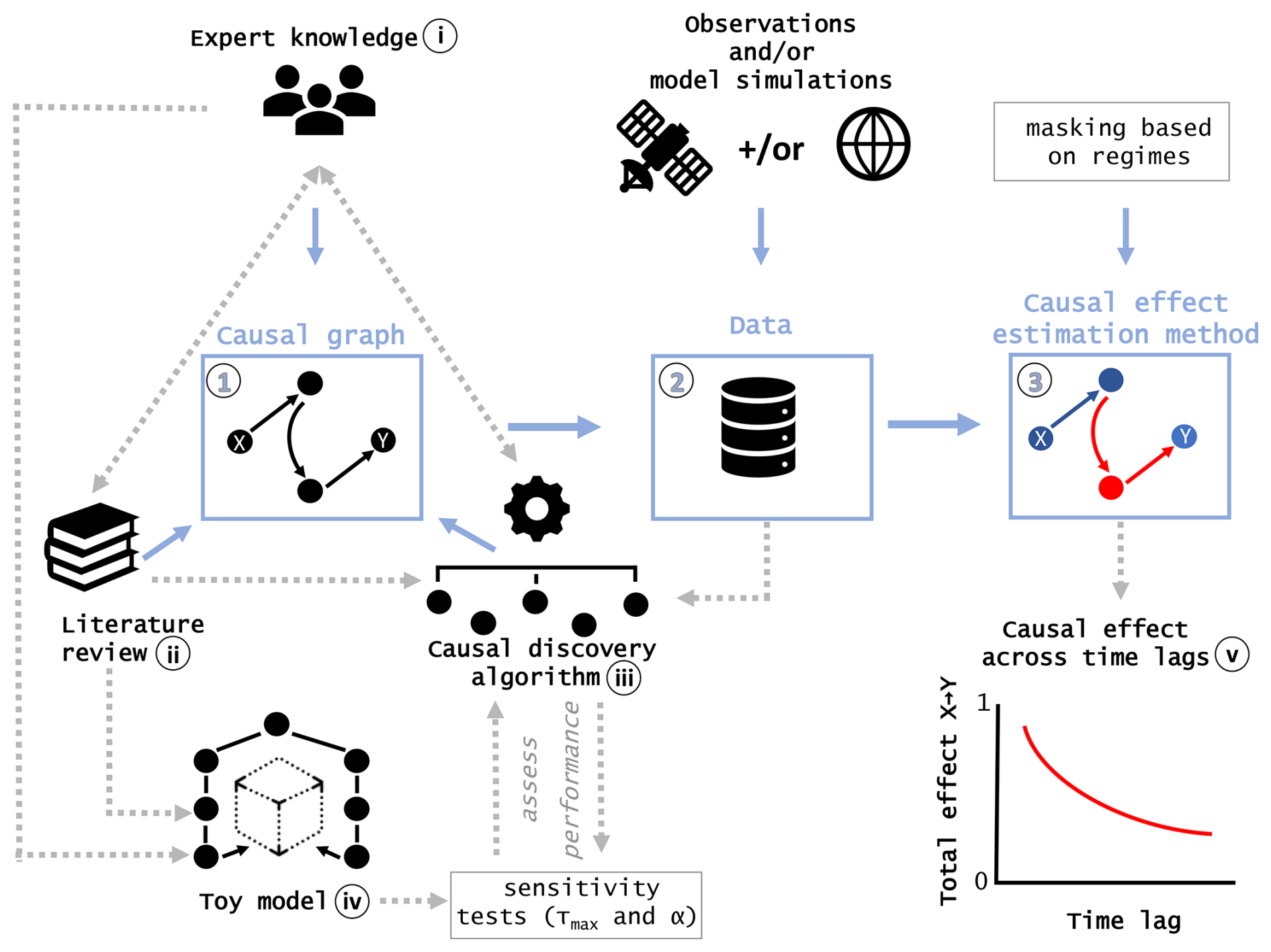
Figure 2 Process-oriented causal inference framework built upon three essential components (blue squares): (1) a causal graph, (2) data, and (3) a method for causal effect estimation. To construct the (1) causal graph for the studied system, a triangulated approach (Uleman et al., 2024) is applied, integrating (i) expert knowledge, (ii) a literature review, and (iii) a data-driven causal discovery algorithm. Before applying the (iii) causal discovery algorithm to real-world data, we construct a (iv) toy model to assess the performance of the selected (iii) causal discovery algorithm. The final (1) causal graph, based on (2) real-world data, serves as a foundation for estimating (3) causal effects, which can be further refined through process-oriented analysis, including masking on atmospheric regimes and additional sensitivity tests.

Figure 2 outlines the process-oriented causal inference framework, which is built upon three essential components (blue squares): (1) a causal graph that contains information about qualitative cause-and-effect relationships (Runge et al., 2023), (2) observational and/or modeled data, and (3) a method for estimating causal effects. To construct (1) the causal graph, we employ a triangulated approach (Denzin, 2010; Uleman et al., 2024) that integrates (i) expert knowledge, (ii) a comprehensive literature review, and (iii) a data-driven causal discovery algorithm. While each of these components can independently contribute to the creation of the causal graph, we recommend employing the triangulated approach to ensure a more robust and reliable framework. To assess the performance of the selected (iii) causal discovery algorithm before applying it to real-world data, we first construct a (iv) “toy model” using synthetic data. This synthetic dataset is designed to replicate the properties and challenges of the real system while incorporating known underlying ground truth from (i) expert knowledge and (ii) a literature review. The toy model is then used to evaluate the performance of the causal discovery method in realistic, finite sample scenarios (Camps-Valls et al., 2023). To ensure the robustness of the results, it is recommended to further perform sensitivity tests on free algorithm parameters, such as α_pc and τ_max for (iii) the causal discovery algorithm and (iv) the toy model.

It is important to note that if (iii) the causal discovery algorithm does not robustly detect anticipated relationships in the analyzed (2) real-world or modelled data, the user can integrate physical knowledge into the algorithm. Alternatively, the causal graph may be constrained purely based on (i) expert knowledge and (ii) a comprehensive literature review, including previous successful applications of causal discovery to related research topics. The final (1) causal graph, derived from (2) real-world data, serves as a foundation for estimating (3) direct and total causal effects. Causal effect estimation can be further refined through a process-oriented analysis, such as, for example, masking on different atmospheric regimes. Additionally, (v) total causal effects can be assessed across different time lags. This complex approach outlined in Fig. 2 ensures robust and reliable causal inference, particularly for complex systems such as the stratospheric chemical-dynamical interactions investigated here.

3.4 Confidence intervals and masking for regime-oriented analysis

Confidence intervals for direct causal effect estimates, computed using Wright's path coefficient (Sect. 4.2), were obtained via bootstrapping with 500 repetitions. Only significant direct causal effects are shown, defined as those for which the bootstrap confidence interval does not include 0. For both direct and total causal effects across different time lags (Sect. 4.4), confidence intervals were also obtained from 500-member bootstrapping. Because the causal effect estimates were conducted on the same data as the prior causal discovery step, the confidence intervals do not cover the uncertainty from this prior model-selection step. In our case, this issue is less pronounced because the causal graph was based on a triangulation and not fully data-driven.

For the regime-oriented analysis of causal effects during different QBO phases (Sect. 4.3), we first calculate the QBO wind shear as the vertical gradient of the zonal mean zonal wind between 10 and 30 hPa. For observations, the shear is derived directly from radiosonde-based zonal wind at the two pressure levels (Kerzenmacher and Braesicke, 2026). For the TOMCAT CTM simulation, the zonal wind is first averaged over 10° S–10° N before computing the vertical gradient between 10 and 30 hPa. The resulting shear time series is subsequently standardized for use in the process-oriented causal analysis. Positive (negative) values correspond to a westerly (easterly) shear zone, which plays a key role in modulating secondary circulation and stratospheric transport. We focus on the 10–30 hPa shear layer since no data is available above 10 hPa in the observational record used here.

4 Results and Discussions

4.1 Causal justification and validation with a toy model

Before applying causal discovery to analyze chemical–dynamical interactions using observations and the TOMCAT CTM simulation, we first summarize the relationships of O₃ variability in this region in a shape of DAG-based on expert knowledge and literature review (as discussed and interpreted by e.g. Galytska et al., 2019; Nedoluha et al., 2015), following the procedure discussed in Sect. 3.3. Figure 3a depicts a simple linear chain from the cause w^* to the outcome O₃ (grey nodes), with mediating variables N₂O and NO₂ (magenta nodes). The inferred DAG, therefore, represents an effective causal structure that emerges under the influence of dynamical variability, rather than a representation of isolated chemical relationships. In particular, a positive relationship from w^* to N₂O (labelled A) indicates that an increase in residual vertical velocity leads to enhanced N₂O concentrations. The relationship from N₂O to NO_x (labelled B) is negative, despite N₂O being a source of NO_x. This apparent contradiction is an example of Simpson's paradox (Blyth, 1972) and arises because tropical residual velocity w^* acts as a confounding dynamical process, leading to an anti-correlation between N₂O and NO₂. Namely, slower (faster) upwelling results in lower (higher) N₂O concentrations and consequently longer (shorter) N₂O residence time in this region, which allows more (less) time for the photochemical production of NO_x from N₂O. Consequently, higher (lower) NO_x levels lead to lower (higher) O₃ concentrations via the NO_x-catalyzed O₃ destruction cycle, resulting in a negative relationship (labelled C, see Crutzen, 1970). Table 1 summarizes the discussed chemical-dynamical relationships in the tropical middle stratosphere as depicted in Fig. 3a.

We further justify the assumed causal DAG in Fig. 3a and validate the reliability of the causal inference method. For this, we require a benchmark dataset with known causal ground truth for validation as depicted in Fig. 3a. We consider the linear structural causal process with four time series as an example that comes from a data-generating process using the following model:

$$\begin{array}{}\text{(1)}& \begin{array}{rl}{X}_t^{\mathrm{0}}& =\mathrm{0.3}{X}_{t-\mathrm{1}}^{\mathrm{0}}+{\mathit{\eta }}_t^{\mathrm{0}}\\ X_t^{\mathrm{1}}& =\mathrm{0.3}{X}_{t-\mathrm{1}}^{\mathrm{1}}+\mathrm{0.4}{X}_{t-\mathrm{1}}^{\mathrm{0}}+{\mathit{\eta }}_t^{\mathrm{1}}\\ X_t^{\mathrm{2}}& =\mathrm{0.3}{X}_{t-\mathrm{1}}^{\mathrm{2}}-\mathrm{0.94}{X}_t^{\mathrm{1}}+{\mathit{\eta }}_t^{\mathrm{2}}\\ X_t^{\mathrm{3}}& =\mathrm{0.3}{X}_{t-\mathrm{1}}^{\mathrm{3}}-\mathrm{0.95}{X}_t^{\mathrm{2}}+{\mathit{\eta }}_t^{\mathrm{3}}\end{array}\end{array}$$

where ${\mathit{\eta }}_t^{\cdot }$ stands for the independent Gaussian white noise processes with variances ${\mathit{\sigma }}_{\cdot }^{\mathrm{2}}$, X⁰ depicts residual vertical velocity w^*, X¹ – the concentration of N₂O, X² – NO_x, X³ – O₃. This set of variables and their dependencies define a toy model. Although this toy model is designed to replicate causal dependencies in the tropical middle stratosphere, it is important to emphasize that there are multiple approaches to constructing such a model. While additional variables could be further introduced based on expert knowledge and a thorough literature review, the goal of the analysis here is not to maximize the number of variables but to create an intuitive system that can simply and effectively replicate the processes under study.

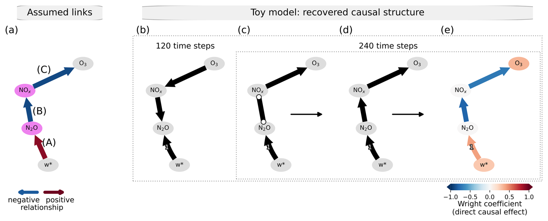
Figure 3 Causal justification and validation. (a) Assumed relationships based on expert knowledge and literature review. Magenta nodes indicate mediators in the total influence of w^* on O₃. (b–e) Causal discovery applied to a generated toy model with contemporaneous (time lag = 0) and lagged (time lag >0) dependencies based on linear partial correlation as a conditional independence test for 120 time steps (b) and 240 time steps (c), which corresponds to the DPAG. The application of the triangulated approach from Fig. 2 resulted in the DAG (d), which in turn was used as a basis for causal effect estimation, where edge colors indicate the estimated direct causal effects (e).

Table 1 Summary of chemical-dynamical processes in the tropical middle stratosphere.

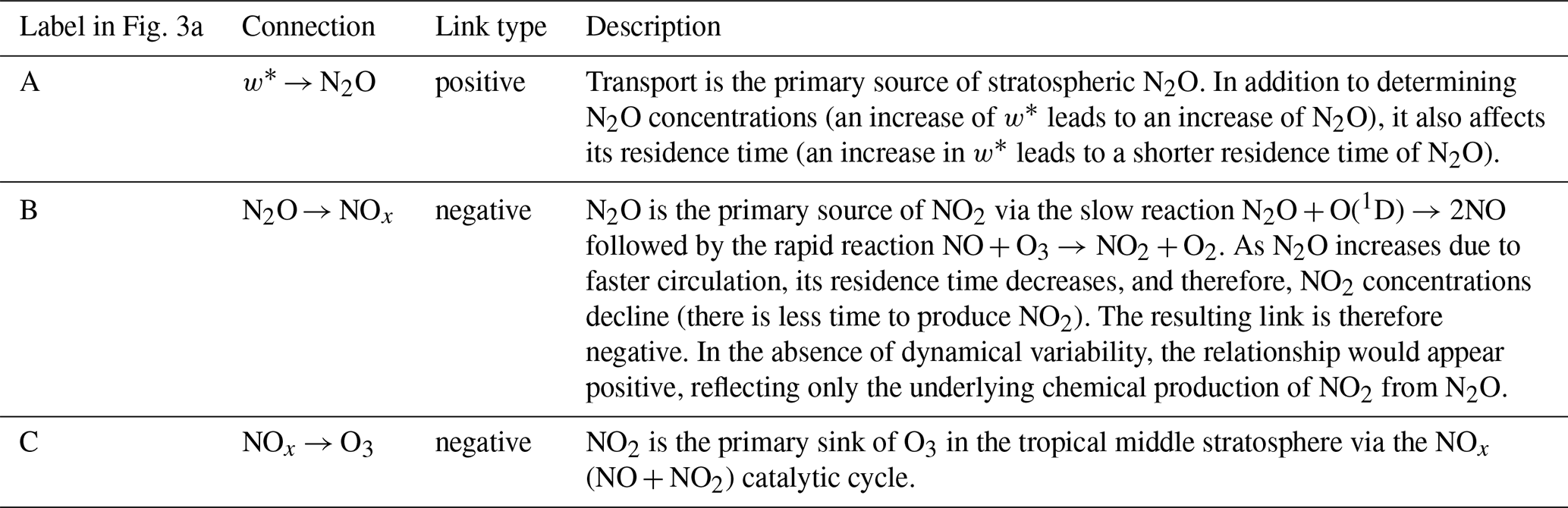
Figure 3b–e illustrate the causal graphs inferred from the causal discovery algorithm (see Sect. 3.1) when applied to the toy model from Eq. (1). To evaluate the performance of the causal discovery algorithm on time series of different lengths, Fig. 3b, c show causal graphs for generated time series of 120 time steps (equivalent to 10 years of monthly data) and 240 time steps (equivalent to 20 years), respectively. When applied to the shorter time series (Fig. 3b), causal discovery fails to detect several expected connections as anticipated from Fig. 3a, likely due to limitations in the toy model, such as weaker causal signals or higher noise. In contrast, despite the plausible limitations of the toy model, most expected connections are recovered in the 20-year time series depicted in Fig. 3c. However, the inferred graph lacks directionality between N₂O and NO₂ (shown as $\circ \text{-}\circ$ edge), resulting in a DPAG. Since causal effect estimation requires a fully directed DAG, we applied the triangulation approach to resolve ambiguities, yielding the DAG in Fig. 3d. This final causal graph (Fig. 3d) serves as the basis for causal effect estimation, shown in Fig. 3e. Given approximately linear relationships among analyzed variables (see Fig. 1b–d), we assume linear causal effects and apply Wright’s method (Wright, 1921). This approach is akin to linear regression slopes between two variables X and Y, with the critical distinction that the graph is used to detect and eliminate confounding influences before regression (see Sect. 3.2 and Fons et al., 2023).

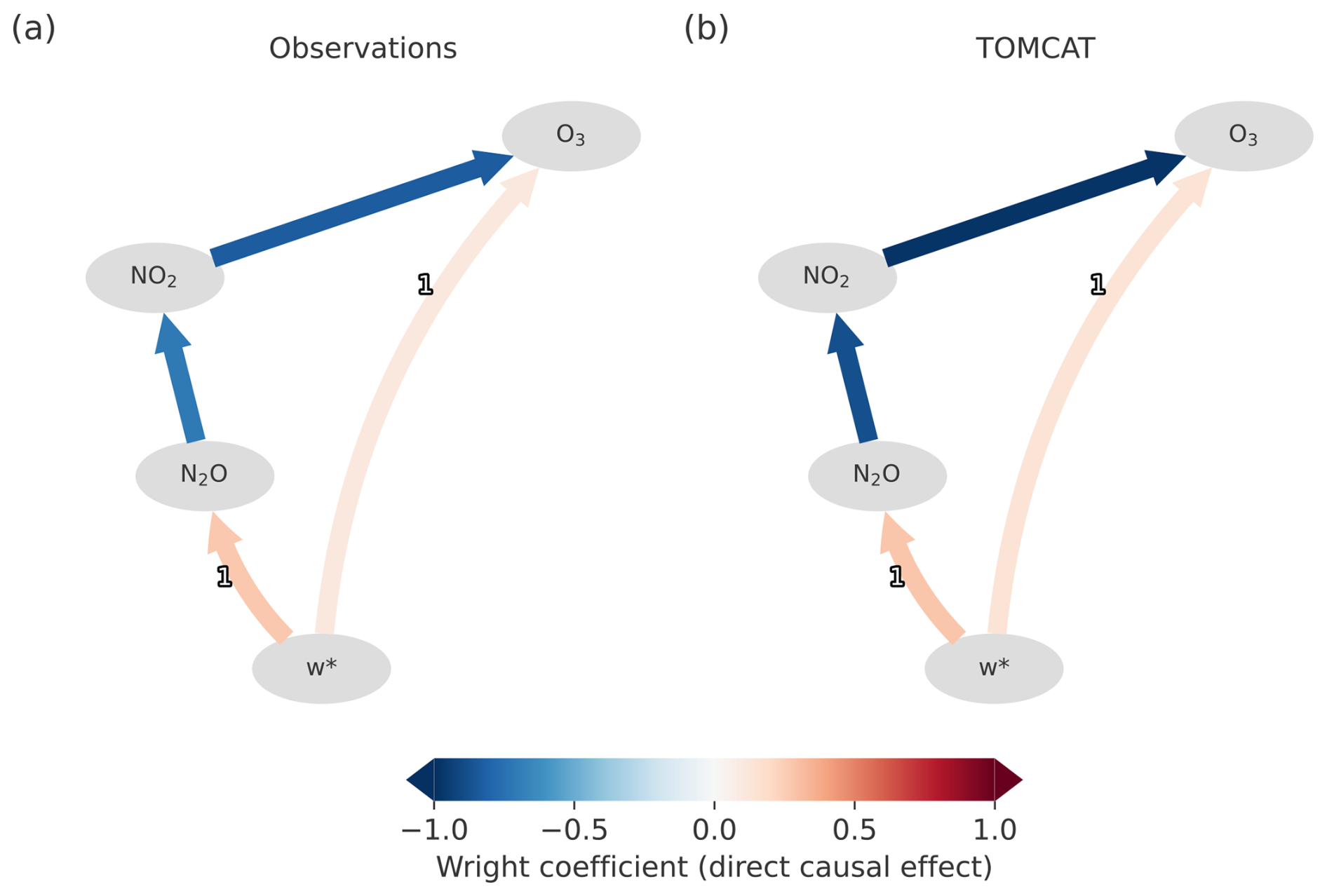
Figure 4 Causal inference: Magnitude and sign of the direct causal effects. The direct causal effects calculated for (a) the observations and (b) the TOMCAT CTM simulation from the detrended monthly anomalies for 2004–2021. Straight arrows show the contemporaneous (time lag = 0) connections; curved arrows indicate lagged links (time lag >0); edge color stands for the estimated direct causal effects. For TOMCAT, causal graphs identified from the observations were used, and direct causal effects were estimated using the TOMCAT data.

4.2 Physical description of observed and modeled causal relations

Figure 4 presents the magnitude and sign of direct causal effects computed using Wright's approach (Wright, 1921) on causal graphs identified by the triangulation (Uleman et al., 2024) based on observations (a) and the TOMCAT CTM simulation (b) during 2004–2021. The original graphs inferred by the causal discovery algorithm (see Sect. 3.1) without the application of the triangulated approach are shown in Appendix C. The causal discovery algorithm successfully identifies the anticipated connections in the observations (Fig. 4a) since the signs of the direct causal effects align well with the expected processes outlined in the Introduction and as discussed in Sect. 4.1.

Notably, the positive lagged link in observations from w^* to N₂O indicates that an increase in residual vertical velocity intensifies N₂O transport. This enhanced transport, in turn, reduces the residence time of N₂O, leading to less time for NO₂ production via the reaction ${\mathrm{N}}_{\mathrm{2}}\mathrm{O}+\mathrm{O}{(}^{\mathrm{1}}\mathrm{D})\to \mathrm{NO}+\mathrm{NO}$ (also labelled B in Fig. 3a). Consequently, the causal contemporaneous link from N₂O to NO₂ reflects the negative relationship confounded by upwelling. The negative contemporaneous link from NO₂ to O₃ indicates that lower/higher NO₂ levels are associated with higher/lower O₃ concentrations, as O₃ loss in the tropical middle stratosphere is largely driven by catalytic destruction by NO_x. Causal discovery further detects a bidirected connection between w^* and O₃ in the observations, indicating the presence of a latent common driver of w^* and O₃ and that neither variable is an ancestor of the other (see Appendix C, Fig. C1a). As causal effect estimation requires a DAG, we define the direction from w^* to O₃ to quantify the strength of this link. This choice allows us to estimate the direct dynamical influence of w^* on O₃, which is sometimes identified by a causal discovery algorithm in sensitivity tests. Based on Fig. 4, the direct influence of w^* on O₃ is much weaker, and a mediated pathway via N₂O and NO₂ dominates. However, temperature-mediated effects could amplify the apparent strength of the connection from NO₂ to O₃, since enhanced upwelling induces both cooling (increasing O₃) and reduced NO_x species. To assess this, we performed additional analysis, including temperature anomalies in the tropical middle stratosphere. The inferred graph structure was not robust, likely because w^* is a derived diagnostic that depends on thermodynamic fields. Removing w^* altered the parent structure and prevented a direct comparison of direct causal effects shown in Fig. 4a. We therefore interpret the identified NO₂-mediated pathway as the dominant mechanism, while acknowledging that temperature-related effects may potentially project onto this link.

Unlike the observations, in the TOMCAT CTM simulation, the causal discovery algorithm does not fully reproduce the expected chemical-dynamical coupling as outlined in the Introduction, Sect. 4.1 and as shown in Fig. 4a. In particular, the anticipated one-month lagged link from w^* to N₂O is not robustly detected. We found that this occurs because O₃ exhibits very strong contemporaneous coupling with both N₂O and NO₂, such that conditioning on O₃ makes the one-month lagged w^* to N₂O link statistically insignificant. As further demonstrated and discussed in Appendix C, this does not indicate a lack of dynamical coupling in the TOMCAT CTM simulation. Instead, it reflects the strong shared variability among the chemical tracers as the model uses a chemically consistent scheme for all the variables. In order to still assess the strength of the processes represented in TOMCAT, we therefore did not rely on the TOMCAT-derived graph. Instead, by adopting a fixed graph structure derived from observational ground truth and expert knowledge, we can accurately estimate direct causal effects with the TOMCAT data (Fig. 4b), providing a valid and pragmatic solution for quantifying model sensitivities. Similar to observations, the direct one-month lagged w^*-N₂O connection is estimated as significant in the TOMCAT CTM simulation for the analyzed period. Additionally, the N₂O-NO₂ negative contemporaneous link is slightly stronger in the TOMCAT CTM simulation (Fig. 4b) compared to those in the observations (Fig. 4a), with a similar causal pattern observed for the NO₂-O₃ link.

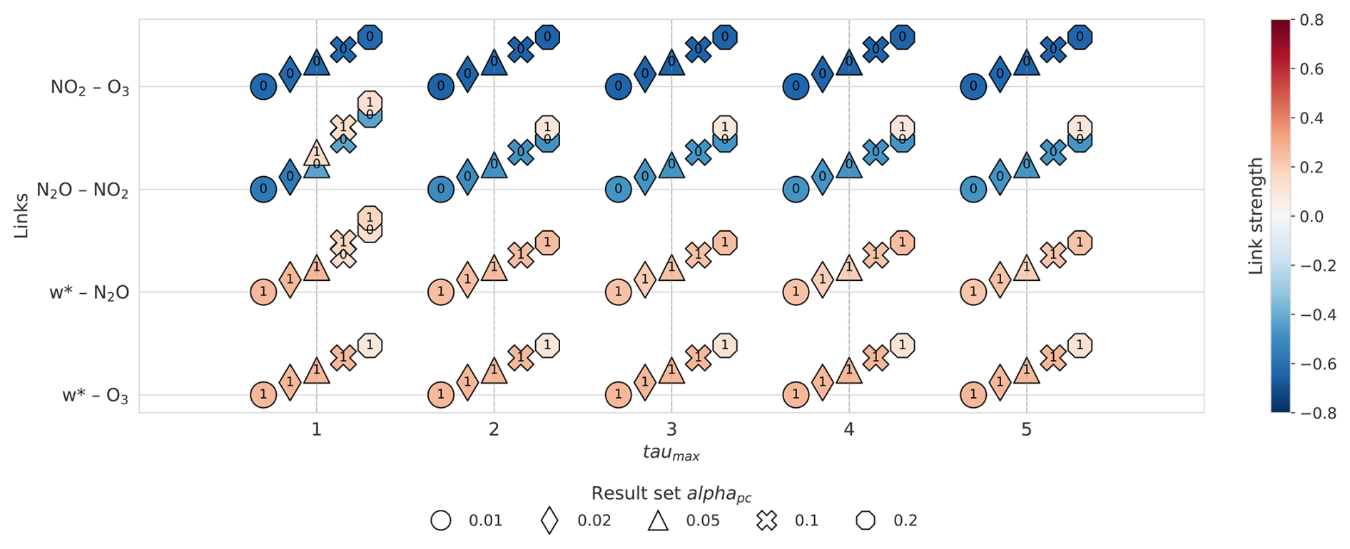
Figure 5 Sensitivity tests of the detected links to the choice of τ_max (x axis) and α_pc (depicted with markers) for the observations for the period 2004–2021. For all tests, the minimum time delay τ_min=0. Only link pairs shown in Fig. 4 are considered.

To ensure the robustness of the connections detected in Fig. 4a in observations in the tropical middle stratosphere during the period 2004–2021, Fig. 5 demonstrates the results of the application of the causal discovery algorithm with different setups of τ_max (depicted on the x axis) and α_pc (depicted with markers). τ_min is set to zero to account for the contemporaneous connections. It should be noted that choosing a τ_max that is too low risks missing causal links with longer delays, which violates the assumption of causal sufficiency. However, choosing τ_max too high without mitigation can dilute the detection power of the causal algorithm. Specifically, a larger τ_max expands the search, as the algorithm tests more possible lagged pairs. This leads to larger conditioning sets, which can further reduce the effect size and detection power. Therefore, it is important to condition only on a few relevant variables that actually explain the relationship (Runge et al., 2019b). Sensitivity tests from Fig. 5 show very similar results for different configurations of τ_max and α_pc. The chemical connections related to N₂O-NO₂ and NO₂-O₃ pairs are robustly detected as contemporaneous across all experiments. The dynamical connections w^*-N₂O and w^*-O₃ are robustly detected with a one-month lag.

A further analysis of the sensitivity experiments reveals an additional feature in the N₂O-NO₂ relationship. A positive one-month lagged link from N₂O to NO₂ is detected across all tested τ_max, but primarily at relaxed significance thresholds (α_pc=0.2). For τ_max=1, the link is also identified at α_pc=0.1 and 0.05. Such a positive lagged connection is physically plausible, as NO₂ is produced from N₂O, as discussed in Table 1, and a delayed response may emerge at the monthly timeseries. However, given its sensitivity to the choice of α_pc, this link cannot be considered a robust pathway.

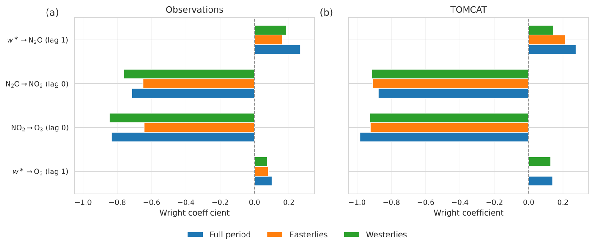
Figure 6 Regime-oriented direct causal effects from (a) observations and (b) the TOMCAT CTM simulation for the full 2004–2021 period (blue), and for easterly (orange) and westerly (green) QBO regimes.

4.3 Process-oriented analysis

We adapt the process-oriented causal analysis (Nowack et al., 2020; Karmouche et al., 2023; Eyring et al., 2024; Debeire et al., 2025) to major drivers of tropical middle stratospheric O₃ variability to further understand the robustness of the connections during different regimes. Given that N₂O, NO₂, and O₃ exhibit a strong QBO signal (Chipperfield et al., 1994; Tian et al., 2006; Park et al., 2017; Ming et al., 2025), we mask the data to easterly and westerly shear zones (see Sect. 3.4). This approach makes it possible to explore the regime-dependent robustness of causal relationships. A robust connection between specific variables indicates that the particular link is consistently detected across multiple resampled datasets. A robust connection also suggests that the relationship is less sensitive to variations in the data, providing higher confidence that the detected connection is not a result of random fluctuations or sampling variability. It is also important to note that the analyzed period includes an unprecedented QBO disruption in 2016 (Tweedy et al., 2017; Match and Fueglistaler, 2021), which stalled the descent of the easterly shear toward 10 hPa and caused anomalous upwelling and wind patterns, temporarily altering transport and mixing in the tropical middle stratosphere. To assess how QBO phase affects the strength of the identified relationships, we keep the causal graph inferred from the full period and re-estimate the link strengths separately for easterly and westerly QBO conditions. This approach isolates regime-oriented changes in coupling strength without altering the underlying network structure. Figure 6 illustrates the estimated direct causal effects for both observations (panel a) and the TOMCAT CTM simulation (panel b) for the full period 2004–2021 (blue), which also corresponds to direct causal effects shown in Fig. 4a,b, easterly (orange), and westerly phase of the QBO.

The dynamical positive link from w^* to N₂O at a lag of one month shows slightly reduced magnitude in observations when separating into QBO phases compared to the full period. In the TOMCAT CTM simulation, the link strength is similar to observations and also slightly reduces across QBO phases. The negative contemporaneous chemical coupling between N₂O and NO₂ is stronger in the TOMCAT CTM simulation compared to observations and of similar strength across phases. In observations, the absolute magnitude is slightly larger during the westerly phase than during the easterly phase. The contemporaneous negative link from NO₂ to O₃ is likewise stronger in the TOMCAT CTM simulation compared to the observations. In the observations, this link weakens during the easterly QBO phase, whereas in the TOMCAT CTM simulation its magnitude is comparatively stable across QBO phases.

The imposed one-month lagged connection from w^* to O₃ is the weakest among the analyzed pathways and substantially smaller than the chemically mediated pathway. In the TOMCAT CTM simulation, no link is detected for the easterly QBO phase. This phase-dependent absence of this connection points to its limited robustness. This also indicates that the direct influence of the residual circulation on O₃ variability is predominantly mediated through N₂O and NO₂, rather than through a direct dynamical effect. Overall, the sign of all connections is robust across datasets and QBO phases. In the observations, the chemical links (from N₂O to NO₂ and from NO₂ to O₃) tend to strengthen during the westerly QBO phase.

4.4 Causal effects across different time lags

While the causal discovery algorithm, along with causal effects estimation of the direct links, offers a general overview of whether the methodology captures the expected dependencies, one can further study the propagation of causal effects through the causal graph across different time lags. The total causal effects (for further discussions, see Appendix D), which are not necessarily just depicted by a single arrow in the causal graph, can be derived from direct causal effects using Wright's path analysis for specific relationships across different time lags. Figure 7 shows total (lines) and direct (labels) causal effects across different time lags for a selection of different (X, Y) pairs of variables, where a positive connection, similar to Fig. 4, indicates that an increase in X leads to an increase in Y after a time lag (τ). Due to the limited number of variables in the causal graphs, we do not analyze the role of mediators for specific connections, as their influence is straightforward. For example, the total causal effect from w^* to NO₂ is mediated solely by N₂O, as shown in Fig. 4. However, for the analyses that involve more complex causal graphs, similar to Fons et al. (2023), we recommend estimating the contribution of various mediators on a specific set of connections.

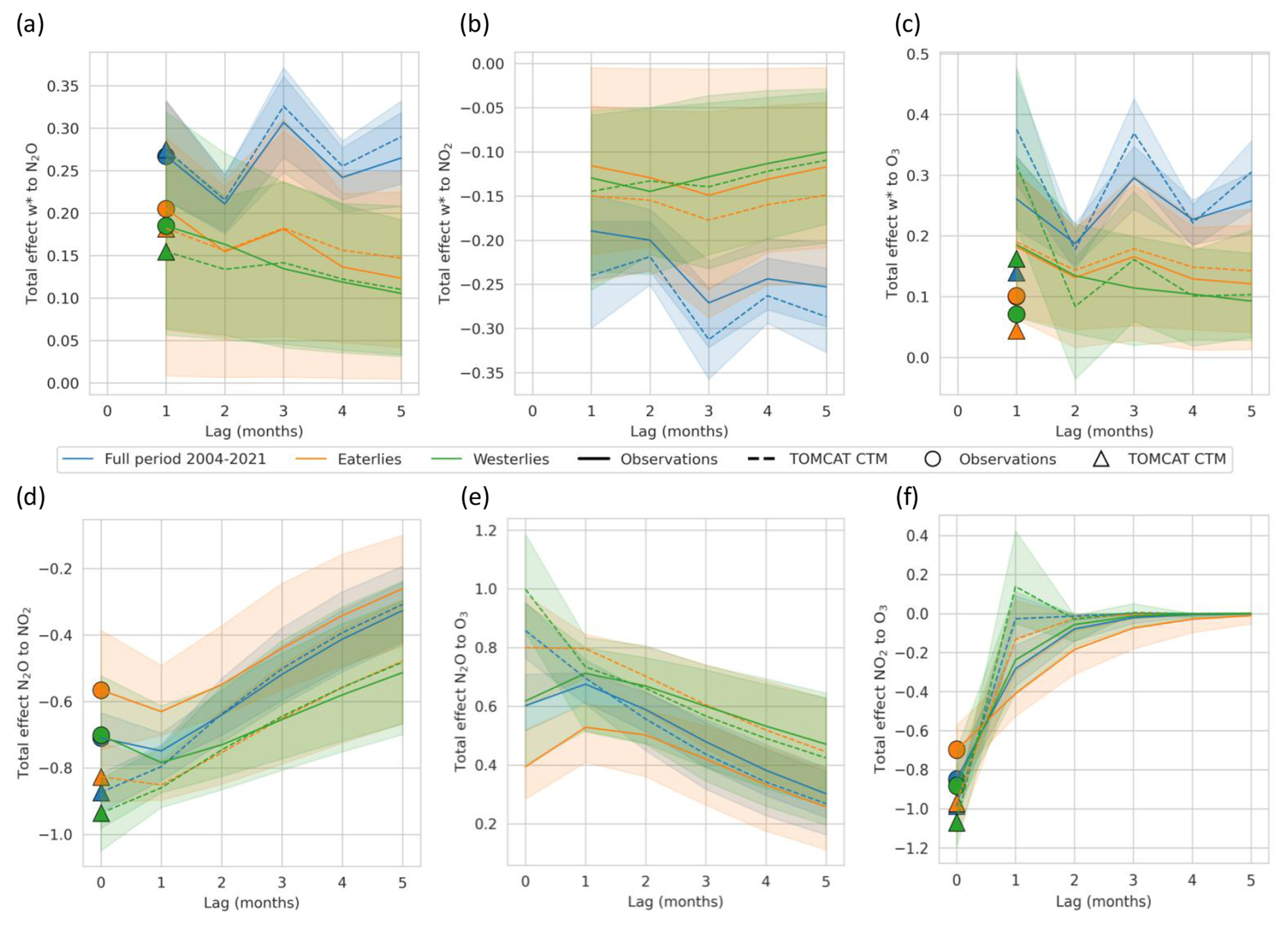
Figure 7 Total causal effects across different time lags in months from observations (solid lines) and the TOMCAT CTM simulation (dashed) for (a) w^* on N₂O, (b) w^* on NO₂, (c) w^* on O₃, (d) N₂O on NO₂, (e) N₂O on O₃, (f) NO₂ on O₃. All plots show the results obtained for 2004–2021 (blue), easterly (orange), and westerly QBO phase (green). The markers indicate direct causal impact similar to Figs. 4 and 6. The shading corresponds to the 90 % bootstrap confidence interval.

Figure 7 demonstrates that the total causal effects across different time lags in the TOMCAT CTM simulation (dashed lines) closely align with observations (solid lines) across analyzed regimes, indicating that the model reproduces not only the sign but also the temporal structure of the effects. However, the amplitudes in the TOMCAT CTM simulation are slightly larger, suggesting a somewhat stronger coupling between analyzed variables in the simulation. The direct causal effect of w^* on N₂O (Fig. 7a) exhibits a clear maximum at a lag of around three months for the full period 2004–2021. The total causal effects of w^* on NO₂ (Fig. 7b) and on O₃ (Fig. 7c and Appendix D) also show similar lagged maxima for the full period 2004–2021. This lagged behavior likely indicates the spatiotemporal structure of the covariability between w^* anomalies at the analyzed 10 hPa level and below. Upwelling anomalies are primarily governed by the QBO and descend over time with the associated shear zones. As a result, an anomaly in w^* at 10 hPa, originating from higher altitudes, produces an instantaneous but modest local effect on composition, while over subsequent months, it persists and increasingly affects lower altitudes. This leads to a cumulative impact on N₂O, NO₂, and consequently O₃, with a delayed maximum in the total causal effect. The timing of this maximum is therefore linked to the vertical extent of the w^* anomaly and the rate at which QBO shear zones descend.

We can further decompose the total causal effect of w^* on O₃ into direct and indirect contributions. As shown by Figs. 4a and 6a, the direct one-month lagged w^* on the O₃ pathway is approximately 0.10 in the observations and 0.14 in the TOMCAT CTM simulation. The indirect contribution, mediated via N₂O and subsequently NO₂, reaches 0.16 in the observations and 0.23 in the simulation (not shown here). Therefore, the total causal effect of w^* on O₃ shown in Fig. 7c at a lag of one month therefore represents the sum of both pathways, yielding approximately 0.26 for the observations and 0.37 for the TOMCAT CTM simulation over the full analyzed period. The same analysis is performed for the easterly and westerly QBO phases, but an analogous description is not discussed further. Conditioning on both N₂O and NO₂ does not alter the magnitude of the mediated effect, indicating that the dominant indirect pathway proceeds sequentially through w^*, N₂O, NO₂, and O₃.

The N₂O on NO₂ relationship (Fig. 7d) strengthens gradually with increasing lag, with close agreement between observations and the TOMCAT CTM simulation after two to three months. Differences are largest at short lags, where the observational estimate shows stronger variability. The observations suggest that this link appears weaker during easterly QBO shear, linked to vertical ascent due to the strengthening of tropical upwelling (Baldwin et al., 2001). The total N₂O to O₃ effect (Fig. 7e) increases from lag zero to lag one (in the observations) and then gradually decreases toward longer lags. Here, observations also show a weaker total causal effect during easterly QBO phase. These results are also consistent with direct causal effects analyzed for different QBO regimes (see Fig. 6). The NO₂ on O₃ effect (Fig. 7f) peaks at lag zero and rapidly decreases, approaching zero after about one month. This behavior is consistent with fast NO_x-driven O₃ chemistry. A slightly longer persistence during the earlier subperiod suggests a more sustained influence of NO₂ on O₃ during that time.

5 Conclusions

This study applies causal inference to quantify the contributions of chemical-dynamical drivers that control O₃ variability in the tropical middle stratosphere. Using a causal discovery algorithm applied to observations over the 2004–2021 period, we robustly identify a dominant chemical–dynamical pathway, in which variability in residual vertical velocity w^* modulates N₂O, subsequently affecting NO₂ and ultimately O₃. The resulting causal graphs are then used within the causal inference framework to quantify the temporal contribution of specific variables on monthly O₃ variability under different QBO phases and to separate the direct and mediated causal effects. In the TOMCAT CTM simulation, strong shared variability among the chemical tracers limited the ability of the discovery algorithm to detect the expected dynamical coupling. Therefore, we applied observational graphs based on triangulation (Uleman et al., 2024) to estimate causal relationships in the TOMCAT monthly data. This example illustrates a practical workaround for cases where models or datasets do not yield the expected causal structure through discovery. Importantly, estimating direct or total causal effects does not require that the graph be learned by an algorithm since a graph informed by expert knowledge and supported by the literature can serve as a valid alternative (Fons et al., 2023). In our case, the close agreement between the observationally derived graph and the main relationships anticipated from established chemical-dynamical interactions (see Fig. 4 and as discussed in the Introduction) demonstrates that the discovery algorithm can indeed recover the expected structure when applied to suitable data. Additionally, the toy model validation further demonstrates reliability under finite-sample conditions (Sect. 4.1). Therefore, the methodology adopted in this study, which integrates triangulation (Uleman et al., 2024) for the construction of causal graphs and an algorithm for causal effect estimation, demonstrates a comprehensive approach to causal inference. This ensures the robustness of the analyzed system and facilitates the quantification of specific connections in a physically meaningful domain.

Direct causal effects applied to the observations and the TOMCAT CTM simulation reveal that tropical middle-stratospheric O₃ variability is dominated by an indirect NO₂-mediated pathway, consistent with previous studies of chemical–dynamical coupling (see Fig. 4 and e.g. Portmann et al., 2012; Chipperfield et al., 2014; Galytska et al., 2019; Iglesias-Suarez et al., 2021; Prather et al., 2023; Ming et al., 2025). This mechanism of identified connections captures variability under different QBO phases via regime-oriented analysis and is also supported by sensitivity tests. For example, the direct influence of w^* on O₃ is weak and not robust across QBO phases. The total causal effects that consist of direct and mediated pathways peak at a lag of approximately two-three months (as discussed in Sect. 4.4, Fig. 7), associated with the cumulative impact of persistent, vertically coupled w^* anomalies linked to the QBO. The process-oriented analysis for different QBO phases applied to the observations suggests that the chemical links between N₂O and NO₂, and NO₂ and O₃ strengthen during westerly shear compared to easterly shear (see Fig. 6). Additional sensitivity tests, including temperature anomalies in the tropical middle stratosphere, did not yield a robust and interpretable graph. Temperature-related effects may therefore partly project onto the identified NO₂-mediated pathway, but within the present framework their contribution cannot be robustly separated and quantified.

Our study highlights the pivotal role causal inference can play in identifying, disentangling, and quantifying complex physical and chemical-dynamical processes in the stratosphere. This work lays the foundation for extending the application of causal inference to other areas involving complex chemical-dynamical interactions. Given its potential, this approach is particularly valuable for systems with connections that are not well understood. In the scope of the application of causal inference to stratospheric chemical-dynamical research, we emphasize the following limitation to the reader. The present analysis considers variability at a single pressure level of 10 hPa and does not explicitly resolve the vertical structure of the analyzed system. In the tropical stratosphere, where air is continuously ascending, variability at a given level is dynamically linked to conditions at lower altitudes. As a result, within such a single-level framework, the identified total lagged causal effects (discussed in Sect. 4.4) reflect a combination of local processes and effects arising from vertical coupling in the circulation. Some of the further general limitations and challenges are discussed in Runge et al. (2019a); Galytska et al. (2023).

We would like to highlight that an integration of causal reasoning into data-driven science will help us to enhance the understanding of complex processes and will support the development of robust methodologies that combine machine learning with statistical approaches. This integration is especially relevant for Earth and environmental sciences, as it benefits both observational and modelling studies. Causal inference has already proven to be an effective tool for climate model evaluation, particularly by enabling comparisons between causal graphs derived from models and those based on observations. This emerging methodology is gaining traction in process-oriented climate model evaluation (Debeire et al., 2025; Karmouche et al., 2023; Galytska et al., 2023; Nowack et al., 2020) and offers valuable insights into the physical mechanisms driving the varying performance of different models. Notably, causal model evaluation not only identifies physically based connections but can also reveal the processes that are poorly represented in models. We also identify a key direction for future research focused on cross-evaluating the process-oriented performance of different CTMs and coupled CCMs. Such efforts could provide valuable insights into model accuracy and the reliability of CCMs, ensuring that the distribution of simulated species or processes is not driven by incorrect or unknown factors. Additionally, integrating causal inference with well-established statistical methods could further advance stratospheric studies, particularly in analyzing the variability of chemical species. Testing these approaches across different chemical and dynamical processes in various stratospheric regions represents a promising avenue for improving model evaluation and understanding complex interactions.

Appendix A: Glossary

Table A1 summarizes commonly used terms in this manuscript and provides brief examples illustrating their application in this study. For further acquaintance with the terminology, we refer the reader to Runge et al. (2023).

(Gerhardus and Runge, 2020; Runge et al., 2019a)

Table A1 Glossary linking causal inference terminology to stratospheric chemistry context.

Appendix B: Comparison of observations and the TOMCAT CTM simulation

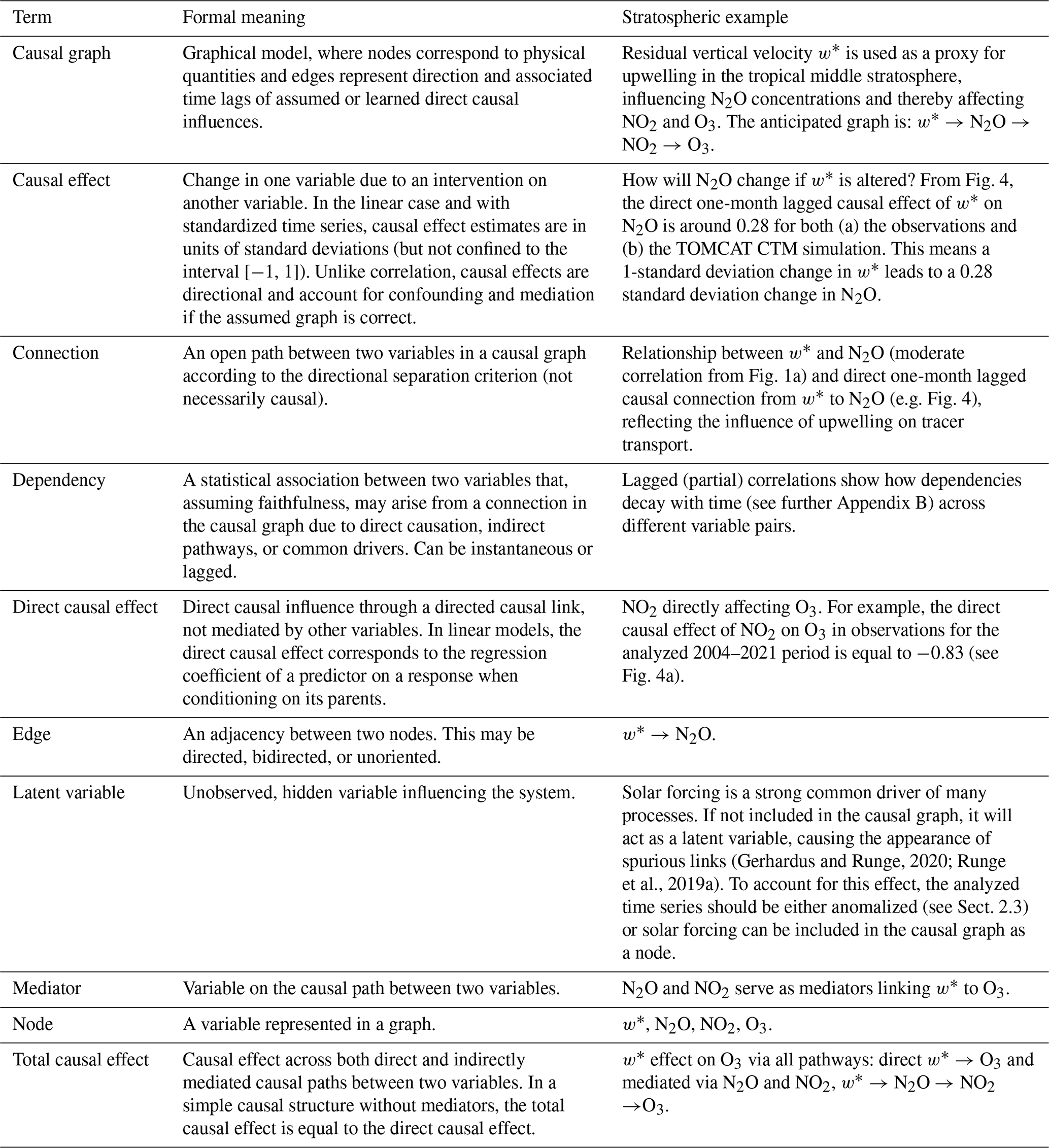
The detrended monthly mean anomalies in the tropical middle stratosphere from observations and the TOMCAT CTM simulation that were used for the causal inference are shown in Fig. B1. Monthly anomalies from the TOMCAT CTM simulation closely align with observations.

Figure B2 depicts lagged dependencies from observations (blue) and the TOMCAT CTM simulation (orange) in the tropical middle stratosphere during 2004–2021 using the RobustParCorr class, i.e., computing lagged correlations after transforming all marginal distributions to Gaussians. Overall, the model reproduces both the sign and the magnitude of the observed relationships across most variable pairs and lags, with correlations generally decreasing in magnitude with increasing time lag. The autocorrelations of the analyzed variables are mostly similar between observations and the TOMCAT CTM simulation, except for NO₂, which exhibits slightly stronger autocorrelation in the TOMCAT CTM simulation across all time lags compared to observations. The connections between w^* and O₃ (first row, last column), N₂O and NO₂ (second row, third column), and O₃ and NO₂ (last row, third column) also show stronger lagged dependencies in the TOMCAT CTM simulation in comparison to observations.

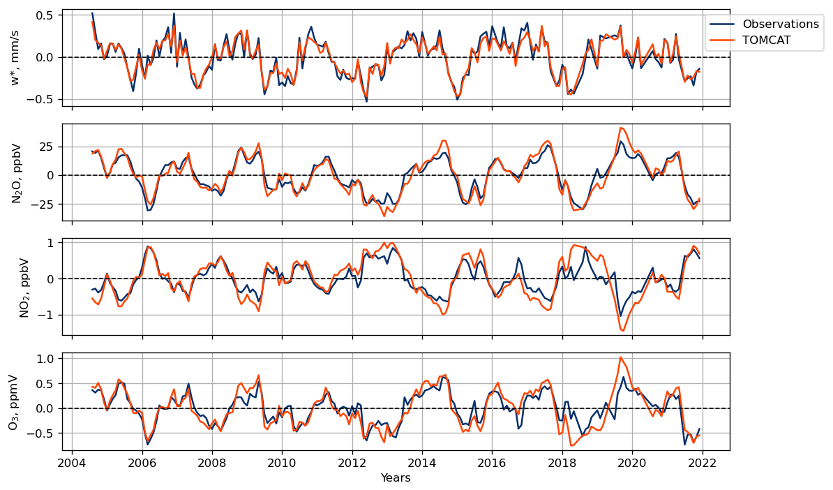
Figure B1 Monthly mean detrended anomalies in the tropical middle stratosphere during 2004–2021 in observations (blue) and the TOMCAT CTM simulation (orange). The TOMCAT CTM data is masked to match the occurrence of the observations.

Figure B3 depicts kernel density estimates of the joint and marginal (diagonal panels) densities of w^*, N₂O, NO₂, and O₃ in the tropical middle stratosphere. Color coding corresponds to Fig. B2. The contours illustrate the covariance structure between the variables, and the annotated τ values indicate the lag at which the strongest association is found. The overall orientation of the contours is similar between observations and the TOMCAT CTM simulation, suggesting that the model captures the main sign of the relationships.

It is important to highlight that the lagged dependencies (Fig. B2) and density plots (Fig. B3) only quantify pairwise co-variability. They do not separate direct from indirect causal effects and do not condition on other variables. Therefore, the lag at which the correlation is strongest should not be interpreted as the lag of a direct causal interaction. In a system with common dynamical forcing and persistence, pairwise correlations can reflect mixed pathways operating on different time scales.

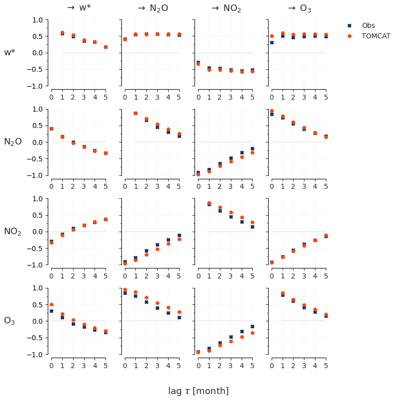
Figure B2 Lagged dependencies in the tropical middle stratosphere during 2004-2021 in observations (blue) and the TOMCAT CTM simulation (orange) based on the RobustParCorr class.

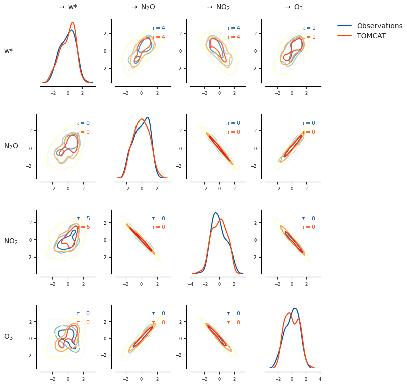
Figure B3 Density estimates of the joint and marginal densities over tropical middle stratosphere during 2004–2021 in observations (blue) and the TOMCAT CTM simulation (orange) based on the RobustParCorr class.

Appendix C: Graphs inferred by the causal discovery algorithm and sensitivity testing

Figure C1 shows the causal graphs detected by the LPCMCI algorithm for the observations (a) and the TOMCAT CTM simulation (b) for the period 2004–2021 with α_pc=0.05 and τ_max=2 in. For the observations, the causal discovery algorithm does not identify the direction of the N₂O–O₃ link. In addition, the w^*–O₃ connection is detected as bidirectional, indicating the presence of a latent common driver of w^* and O₃ rather than a resolved causal direction. For the TOMCAT CTM simulation, in contrast to observations, the causal discovery algorithm does not detect the anticipated negative link from w^* to N₂O, however captures the negative contemporaneous links (without directions) between N₂O and NO₂, and NO₂ and O₃.

Further analysis of the output from the causal discovery from the observations revealed that the algorithm successfully identified a significant lagged causal link from w^* to N₂O, indicating that past values of w^* have a direct influence on N₂O. This relationship remained significant even after conditioning on other variables and their lags, suggesting a robust causal connection. In contrast, in the TOMCAT CTM simulation, the same lagged link was initially detected but became statistically insignificant once O₃ was included in the conditioning set, indicating that O₃ explains most of the shared variability between transport and N₂O. To further investigate the reason for the removal of one-month lagged w^* to N₂O link in the TOMCAT CTM simulation for the period 2004–2021, Fig. C2 shows the results of causal discovery after excluding O₃ from the variable set. In this reduced setup, the w^* to N₂O one-month lagged link reappeared and was statistically significant across tested α_pc. This indicates that the previously missing transport signal is not due to a lack of dynamical coupling in the TOMCAT CTM simulation, but rather to conditional independence induced by the strong covariance among the chemical variables. In the TOMCAT CTM simulation, O₃ has strong instantaneous coupling with both N₂O and NO₂, and therefore accounts for a large part of their common variability. Consequently, once conditioning on O₃, the remaining unique contribution of w^* to N₂O variability is no longer statistically detectable. The re-emergence of the w^* to N₂O link in the reduced system (without O₃) therefore indicates that the transport influence is present, but in the full multivariate setup it becomes statistically hidden because the strongly coupled chemical tracers (O₃ and N₂O, and O₃ and NO₂) explain most of the same variability.

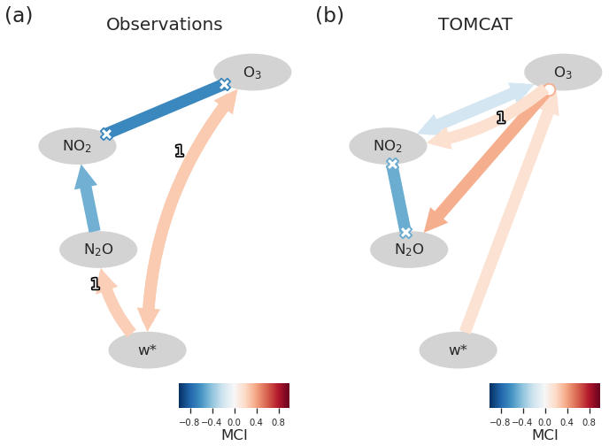
Figure C1 Causal graphs detected by the causal discovery algorithm from (a) observations and (b) the TOMCAT CTM simulation for the period 2004–2021 with significance level α_pc=0.05 and τ_max=2.

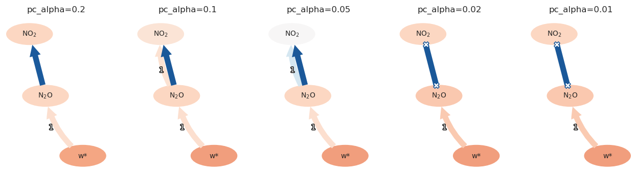
Figure C2 Causal graphs detected by the causal discovery algorithm from the TOMCAT CTM simulation for the period 2004–2021 with different significance levels α_pc and τ_max=2.

Appendix D: Total causal effects

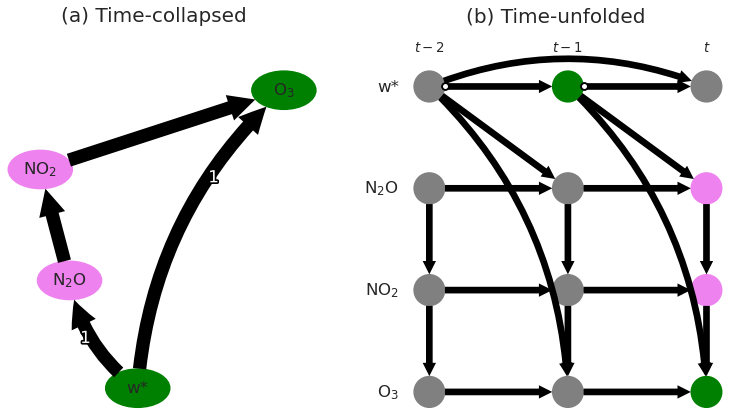
To better understand the causal effects across different time lags, Fig. D1 depicts (a) time-collapsed and (b) time-unfolded causal graphs based on the observational causal graph detected in Fig.4a in the manuscript. As an example, the total causal effect of w^* on O₃ (green nodes) consists of a direct path from w^* to O₃ and an indirect path, which is mediated by N₂O and NO₂ (violet nodes) as shown in Fig. D1a. The indirect path of the influence of w^* on O₃ is then better represented via a time series causal graph (Fig. D1b). The total causal effect across different time lags of this relationship is shown and discussed in Fig. 7c in the manuscript.

Figure D1 Example of the total causal effect of w^* on O₃ (green) as a sum of a direct lagged link and indirect via N₂O and NO₂ mediators (violet) in the time-collapsed graph (a), which corresponds to the causal graph from observations shown in Fig. 4a and time-unfolded graph (b).

Appendix E: Dependencies vs. causal effects across different time lags

The lagged unconditional dependencies, such as the lagged correlations based on partial correlation, are helpful to identify the maximal time lag τ_max to choose in the causal discovery algorithm. However, large autocorrelation might inflate lag peaks (Runge et al., 2014). To condition out some part of the autocorrelation, the bivariate, lagged CI test (partial correlation as an example) can be applied. The comparison between the lagged dependencies from both tests is shown in Fig. E1. We also plot lagged dependencies based on the calculated Wright coefficient (labeled as “causal effects”), which directly indicates the strength of causal relationships and takes into account the direction of causal influence (see, e.g. Fig. 4 in the manuscript). For example, the causal effects in the last row in Fig. E1 are all zero since O₃ is not a cause of any analyzed variable in the system.

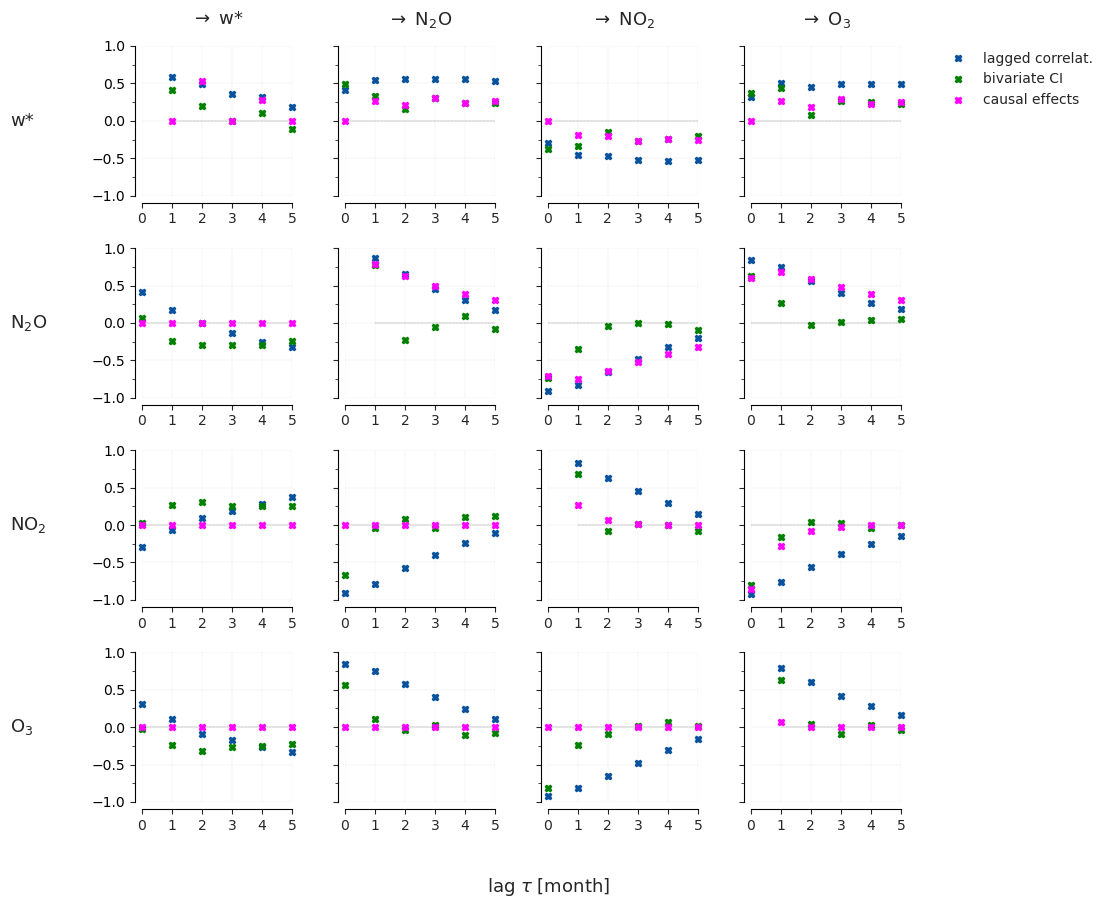
Figure E1 Lagged dependencies across different time lags (in months) from observations for the period 2004–2021 based on partial correlations (blue), bivariate partial correlations (green), and estimated Wright coefficients (magenta).