A modified stratiform cloud microphysics parameterization: evaluation using the Community Atmosphere Model version 6 single-column model

Large-scale stratiform clouds are widespread and dominate the Earth's radiation budget. Their radiative and microphysical properties are inseparable, depending on ambient aerosol conditions and on properties of any convective outflow. In the Community Atmospheric Model, version 6 (CAM6), large-scale clouds were originally treated two decades ago with a two-moment bulk microphysics approach. Since then, the technological and empirical basis of global models has improved, for example by representing cloud microphysics to encompass extra processes of ice and droplet initiation, and by including dependencies on aerosol conditions of size, composition, and loading.

To advance the microphysical realism of the large-scale cloud scheme of the global model CAM6, most of the known mechanisms of secondary ice production (SIP) and an empirical formulation for heterogeneous ice nucleation have been represented in the stratiform scheme of the Global model CAM6. We included a hybrid bin/bulk microphysics scheme that treats aerosol activation, growth processes of accretion, aggregation, and riming, and three SIP mechanisms in the stratiform cloud scheme. We simulated an observed case of a mesoscale convective system during the Mid-latitude Continental Convective Clouds Experiment (MC3E) in Oklahoma, USA, using the Single-Column Atmosphere Model (SCAM6). The results from the simulations are validated against the aircraft, satellite, and ground measurements.

Results show that the modified stratiform scheme can predict the cloud properties of the observed stratiform clouds realistically. Together with our improved convective scheme in CAM6, this paves the way for more realism in the treatment of aerosol-cloud interactions in global climate change by conventional General Circulation Models.

1 Introduction

Cloud parameterisations are essential for climate and weather prediction in conventional General Circulation Models (GCMs). GCMs partition the problem of cloud parameterisation into two distinct broad categories, namely for stratiform and convective clouds. Convective clouds have a strong updraft velocity (>1 m s⁻¹), and stratiform regions have weak ascent (<1 m s⁻¹) with less spatial variability (Houze, 1989; Sui et al., 2007). Convective precipitation is characterised by short duration, high intensity, and rapid fluctuations, on similar scales to the related convective clouds, which are unresolved by conventional global models. Stratiform precipitation is more long-lasting and widespread than convective rain, resulting in significant rainfall accumulation (Houze, 2014).

Stratiform clouds are extensive and characterized by minimal vertical motion. Ensembles of stratiform clouds often cover regions of up to 1000 km in horizontal distance. Their large-scale average properties can be treated as prognostic variables and resolved by global models, although most of the variability of their properties remains unresolved. These clouds greatly influence the Earth's radiative balance by reflecting sunlight back into space and interacting with longwave radiation, resulting in a net cooling effect (Liou, 2002). Simulations from cloud-resolving models accurately estimate cloud properties but tend to underestimate stratiform precipitation (Fridlind et al., 2017; Varble et al., 2014). Various studies have shown that under-prediction in stratiform precipitation by cloud models may be due to biases in treatment of the raindrop size distribution (Li et al., 2009), underestimation of ice water content (Varble et al., 2014), or lack of detrained convective outflow (Bryan and Morrison, 2012).

Microphysical processes involve the conversion of water vapour to different types of hydrometeors in clouds and the transfer of mass among these different types. Liquid hydrometeors are cloud droplets and raindrops; ice hydrometeors are snow, graupel/hail, and cloud ice. Aerosols in the atmosphere act as cloud condensation nuclei (CCN) and a tiny minority of them act as ice nucleating particles (INPs) to initiate cloud droplets and ice crystals, respectively (Petters and Kreidenweis, 2007; Andreae and Rosenfeld, 2008). Secondary ice production (SIP) enhances ice number concentrations from pre-existing ice precipitation particles independently of any aerosol influence (Field et al., 2016; Yang et al., 2016; Korolev and Leisner, 2020). Since the ice and liquid phases in mixed-phase clouds are inter-related through the Bergeron-Findeisen process and by coagulation processes of growth in nature, it is essential to include all ice initiation mechanisms to predict accurately the cloud phase and radiative properties, which subsequently influence cloud coverage and longevity (Sun and Shine, 1994; Field and Heymsfield, 2015; Mülmenstädt et al., 2015; Gupta et al., 2023).

Many observations have shown that ice number concentrations are typically up to four orders of magnitude higher than active INP concentrations for cloud-top temperatures (Harris-Hobbs and Cooper, 1987; Ladino et al., 2017; Lasher-Trapp et al., 2021). Recent studies, including various SIP mechanisms, have demonstrated an improvement in the prediction of ice number concentrations (Sullivan et al., 2017, 2018; Sotiropoulou et al., 2020, 2021; Phillips et al., 2017a; Waman et al., 2022). SIP mechanisms influence the cloud properties such as cloud lifetime, precipitation rate and electrification (Phillips et al., 2017a, b, 2020; Sotiropoulou et al., 2021). Some of the proposed SIP mechanisms (Field et al., 2016) are

1. The Hallett-Mossop (“HM”) process of rime splintering (Hallett and Mossop, 1974)

2. Fragmentation during ice-ice collisions (Vardiman, 1978; Takahashi et al., 1995; Yano and Phillips, 2011; Phillips et al., 2017a; Gautam et al., 2024; Jadav et al., 2025)

3. Fragmentation during raindrop freezing (Dye and Hobbs, 1968; Takahashi and Yamashita, 1977; Phillips et al., 2018)

The HM process is currently controversial as a recent lab study failed to observe it (Seidel et al., 2024). The reason might conceivably be that artificial subsaturation with respect to ice in the airflow around the rimer might have depleted HM splinters before they could be detected in this recent experiment.

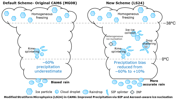
The present paper aims to convey an improved treatment of the interaction between large-scale cloud properties and the aerosol conditions of the environment. A new treatment of mechanisms for cloud droplet and ice crystal initiation is included in the framework of the existing stratiform cloud microphysics scheme by Morrison and Gettelman (2008) and Gettelman and Morrison (2015). We include all of the SIP mechanisms noted above, except for the HM process, which is already treated.

The model development is done using a test-bed consisting of a case of a intensively observed multi-cell storm in the Southern Great Plains of USA from a field campaign in 2011 known as MC3E (Jensen et al., 2016). It was a mesoscale convective system (MCS) consisting of many thunderstorm cells of deep convection. MC3E's multi-platform observational comprehensiveness, integrating satellite simulator remote sensing, cloud penetrating aircraft in-situ observations, ground-based profiling radars, and a dense radiosonde forcing network (6 sites, 1362 launches), has not been replicated in subsequent campaigns. This integrated strategy is essential for validating microphysics parameterizations that depend explicitly on coupling between local cloud processes and large-scale environmental constraints. By using an observed case from this campaign, the present study thus provides not merely historical data, but uniquely comprehensive constraints unavailable from more recent campaigns. Cloud microphysics measurement technology has not advanced meaningfully in the intervening 14 years. All aircraft-based particle probes, droplet counters, and thermodynamic sensors deployed in MC3E, specifically the Cloud Imaging Probe, 2D-C probe, HVPS, Cloud Droplet Probe, hot-wire liquid water content sensors, and Vaisala radiosondes, employ technologies that remain the operational standard in 2024–2025 field campaigns. As evidence, we note that subsequent independent field campaigns (ACAPEX 2019, MARCUS 2018, MICRE 2022, SOCRATES 2018) continue to deploy similar instrument suites with unchanged size specifications and measurement uncertainties, indicating little substantial technological advancement since MC3E.

The paper is structured as follows. Section 2 describes the model and the new microphysical processes represented in it. Section 4 presents the single-column model results using the new scheme, compared with coincident observations and the original version of the model using unmodified stratiform and convection cloud schemes. The main conclusions of this study are summarised in the concluding section (Sect. 6).

2 Model description

2.1 Community Atmosphere Model version 6 (CAM6)

The Community Atmospheric Model, version 6 (CAM6), is the atmospheric component of CESM. The present study uses the Single Column Atmospheric Model, version 6 (SCAM6) which represents a single grid-box column of the global model and utilises the CAM6 physics package (Gettelman et al., 2019). Large-scale tendencies for SCAM6 are prescribed from observations or global simulations. SCAM6 is a valuable tool for developing and testing parameterisations generally.

In CAM6, the original version of the stratiform cloud microphysics scheme followed a two-moment bulk microphysics approach (Morrison and Gettelman, 2008; Gettelman and Morrison, 2015), hereafter “MG08”. The scheme represented four cloud hydrometeor species: cloud liquid, cloud ice, snow and rain. The activation of cloud droplets followed Abdul-Razzak and Ghan (2000). Initiation of ice crystals followed Liu and Penner (2005). The ice number concentration in the stratiform microphysics scheme was limited so as not to exceed the so called “prescribed” value calculated at about −36 °C. For SIP, the original stratiform scheme (MG08) represented only the HM process of rime-splintering, and other SIP processes were omitted.

2.2 Modified representation of cloud microphysics

In this paper, we have modified the stratiform cloud microphysics in the CAM6 global model by including new microphysical processes and changing the representation of certain included processes of stratiform microphysics. The changes are summarised as follows:

1. The microphysics scheme now represents five cloud hydrometeor species: cloud droplets, rain, cloud-ice, snow, and graupel/hail. Graupel/hail mass and number mixing ratios are treated diagnostically instead of prognostically for the purpose of treating microphysical processes such as SIP (HM process, breakup in ice-ice collisions). Since there is no prognostic variable for graupel/hail in the global model (CAM6), its amount is diagnosed for the purpose of treating microphysical processes, according to a look-up table for graupel mass (as a function of cloud-liquid and snow mass mixing ratios and temperature) from high-resolution cloud simulations with the aerosol-cloud model (AC).

2. The cloud base droplet activation is represented by a scheme following Ming et al. (2006), which is more accurate for the treatment of aerosol conditions of chemistry.

3. In-cloud droplet activation of aerosol species is now represented by κ-Kohler theory because it allows internal mixtures (e.g. dust or BC coated with soluble aerosols) to be treated accurately (Petters and Kreidenweis, 2007).

4. Three extra SIP mechanisms noted above (Sect. 1) are included.

5. Growth processes of aggregation, accretion and riming are treated with emulated bin microphysics schemes.

The treatment of stratiform microphysics is qualitatively consistent with the new convective microphysics scheme also for CAM6 (Jadav et al., 2025). In that scheme, deep convection follows the Zhang–McFarlane framework but with the modifications introduced by Jadav et al. (2025): a 6 h convective adjustment time scale, revised triggering including convective inhibition (CIN), replacement of SZ11 microphysics by a detailed aerosol–cloud convection (ACC) microphysical scheme with a high-resolution 1-D plume model, updated entrainment–detrainment formulations, and explicit transfer of detrained cloud liquid, ice, rain, snow, and graupel to the large-scale cloud scheme as prognostic source terms.

The new ACC treatment involved embedding a parcel in which hybrid bin-bulk microphysics routines are applied to treat coagulation, with ascent of the parcel in 1D through each bulk plume, using vertical velocity information derived from the convecective available potential energy (CAPE) in the ZM framework. The known and empirically characterised mechanisms of initiation of droplets and ice particles, pertinent to deep convective ascent, were treated, including three SIP mechanisms, homogeneous freezing of drops, heterogeneous ice nucleation in terms of aerosol conditions of size, loading and composition, and separate explicit treatment of cloud-base and in-cloud droplet activation. The supersaturation in the cloudy parcel was explicitly predicted throughout the ascent, enabling this detailed treatment.

The microphysical treatment of both schemes is related to that in a high-resolution aerosol-cloud (AC) model (Phillips et al., 2007, 2008, 2009, 2013, 2015, 2017a, b, 2018, 2020; Kudzotsa et al., 2016). Both schemes for large-scale cloud, described here, and for deep convection (Jadav et al., 2025) are included in the control simulations of the present paper.

2.2.1 Treatment of aerosol

The aerosol treatment in the modified stratiform scheme follows the framework of Phillips et al. (2009), which was developed to enable explicit representation of ice nucleation dependencies on aerosol composition. This represents a departure from the default CAM6 aerosol module (Liu et al., 2016), which uses a modal approach with four modes (Aitken, accumulation, coarse, primary carbon) and does not track aerosol species with the compositional detail required for heterogeneous ice nucleation parameterizations. There are seven chemical species of aerosols, including both soluble and solid species of aerosol material.

Specifically, the stratiform cloud scheme tracks these chemical species of aerosols, classified into soluble and insoluble categories:

• Soluble aerosol species:

  • Sulphate (2 modes): Accumulation mode (0.8 µm) and smaller mode (height-dependent above PBL), derived from SO₂ oxidation and primary emissions from fossil fuel combustion and volcanic sources

  • Sea salt (3 modes): Geometric mean diameters 0.03, 0.18, and 4.4 µm, representing film drops, jet drops, and spume drops from ocean spray

  • Secondary organic aerosols (2 modes): Geometric mean diameters 0.05 and 0.04 µm, formed through gas-to-particle conversion of biogenic and anthropogenic volatile organic compounds

• Insoluble aerosol species:

  • Mineral dust (2 modes): Accumulation (0.3 µm) and coarse (0.8 µm) modes, from wind-blown desert and agricultural sources

  • Black carbon: Single mode (0.09 µm), primarily from incomplete combustion of fossil fuels and biomass burning

  • Primary biological aerosols: Two modes (0.16 and 0.46 µm), including bacteria, fungal spores, and pollen, emitted from vegetated surfaces

  • Insoluble primary organics: Single mode (0.2 µm), non-biological organic matter from combustion sources including biomass burning

Log-normal size distributions are implemented for all aerosol chemical species (Pruppacher and Klett, 2010). The distribution parameters of the aerosols are given in Table 1 for continental aerosol conditions.

Table 1 Aerosol properties. A comma separates the modes

As in the original CAM6 version, biomass burning contributes to black carbon, primary organics, and partially to organic aerosol loadings. The aerosol emissions are prescribed from the CMIP6 emission inventories (Hoesly et al., 2018), which include explicit biomass burning sectors (agricultural waste, forest fires, peat burning).

Aerosols are depleted by two mechanisms: (1) wet scavenging through in-cloud nucleation (described above) and nucleation scavenging below cloud by precipitation, and (2) dry deposition at the surface following the resistance-in-series approach of Wesely and Lesht (1989) implemented in CAM6. Wet scavenging of aerosols, by activation as cloud-droplets and as ice crystals followed by accretion onto precipitation, is computed prognostically using the present microphysics scheme, as described below. Dry deposition velocities depend on aerosol size, with typical values of 0.1–0.5 cm s⁻¹ for accumulation mode particles and 0.01–0.05 cm s⁻¹ for Aitken mode particles over vegetated surfaces. In the single-column framework, only the wet scavenging is interactive with the microphysics scheme; dry deposition acts as a prescribed boundary condition affecting the column-integrated aerosol burden over the simulation period.

In summary, the treatment of aerosols in the stratiform cloud scheme is consistent with that in the convection scheme described by Jadav et al. (2025), treating the feedback from the cloud onto the aerosol fields. The size distributions of the aerosol species inform the treatment of initiation of cloud-droplets and ice crystals as noted below.

2.2.2 Particle size distribution of hydrometeors

Representations of new microphysics processes follow a hybrid bin/bulk approach.

2.2.3 Bulk approach

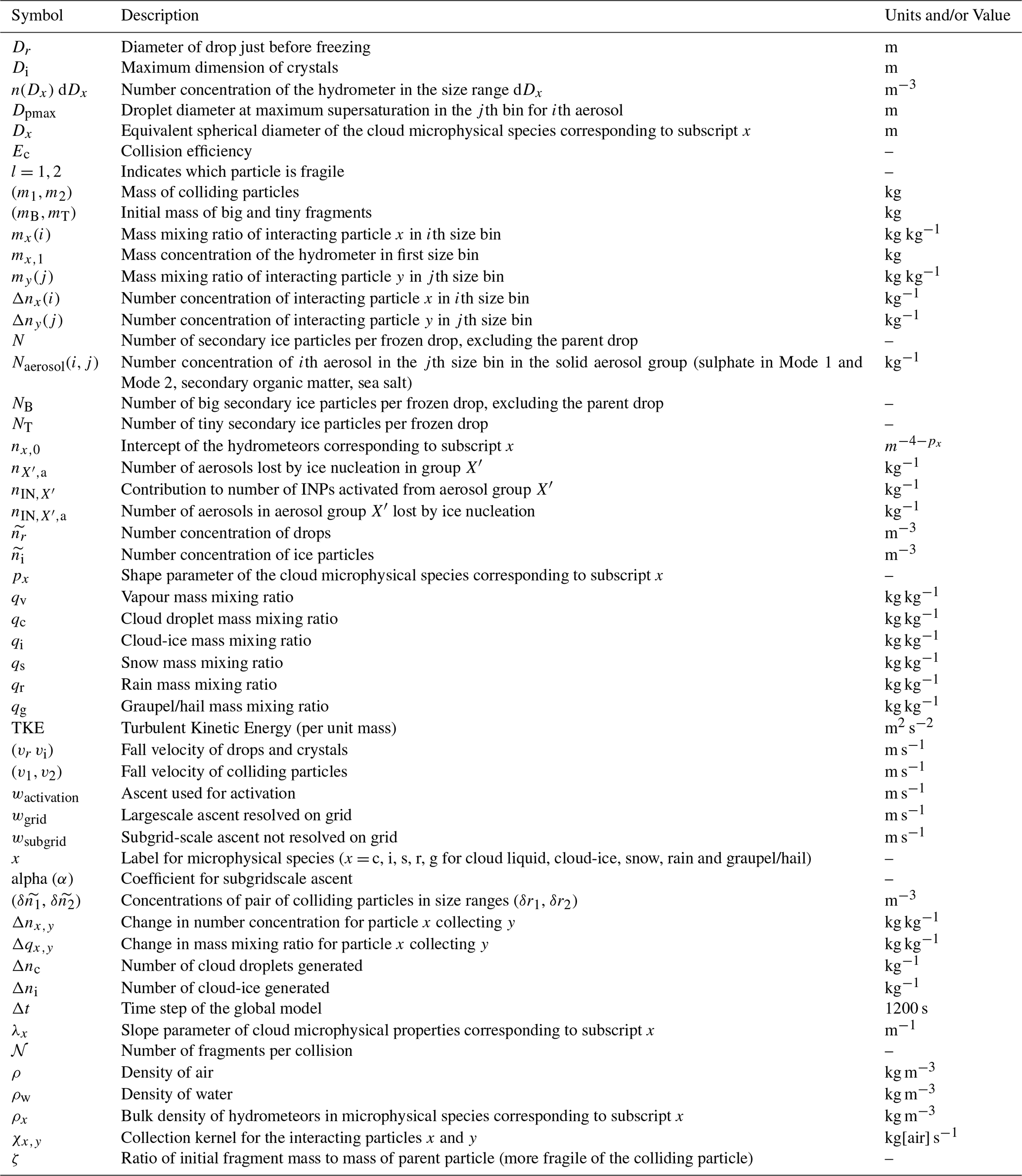
The bulk parameterisation follows a gamma size distribution (Phillips et al., 2007, 2017b):

$$\begin{array}{}\text{(1)}& n\left(D_x\right)=n_{x,\mathrm{0}}{D_x}^{p_x}{e}^{-{\mathit{\lambda }}_x{D}_x}\end{array}$$

Here p_x represents the shape parameter. n_x,0 is from standard formulae (Ferrier, 1994; Morrison et al., 2005), except for snow and graupel, for which lookup tables are used. For cloud liquid, p_w=3.5; for cloud-ice p_i=1; rain has p_r=2.5; and graupel/hail has p_g=1 (Phillips et al., 2007). The shape parameter for snow is calculated from a lookup table that takes into account the size dependence of bulk density and axial ratio (Heymsfield et al., 2002). λ_x represents the slope of the size distribution.

$$\begin{array}{}\text{(2)}& n_x=\underset{\mathrm{0}}{\overset{\mathrm{\infty }}{\int }}n\left(D_x\right)\mathrm{d}{D}_x/\mathit{\rho }\end{array}$$

The mass mixing ratio for cloud liquid, cloud-ice is given as,

$$\begin{array}{}\text{(3)}& q_x={\displaystyle \frac{\mathit{\pi }}{\mathrm{6}}}\underset{\mathrm{0}}{\overset{\mathrm{\infty }}{\int }}{\mathit{\rho }}_x{D}_x^{\mathrm{3}}n\left(D_x\right)\mathrm{d}{D}_x/\mathit{\rho }\end{array}$$

Here x= c, i, r, s, g represent hydrometeor species. n_x and q_x are the hydrometeor's number and mass mixing ratios. ρ_x is the bulk density of the hydrometer. D_x is the equivalent spherical diameter and n(D_x)dD_x is the number concentration (m⁻³) of cloud hydrometeors in size range dD_x. For species with constant bulk density, independent of size, the slope parameter of the size distribution is given by:

$$\begin{array}{}\text{(4)}& {\mathit{\lambda }}_x=\left[{\displaystyle \frac{\mathrm{\Gamma }(\mathrm{4}+p_x){\mathit{\rho }}_x\frac{\mathit{\pi }}{\mathrm{6}}{n}_x}{\mathrm{\Gamma }(\mathrm{1}+p_x)q_x}}\right]\end{array}$$

Here, Γ is the gamma function (see also Ferrier, 1994, Morrison et al., 2005 ). However, for snow and graupel/hail, the bulk density is an empirical function of size and so a lookup table is used for λ_x as a function of $q_x/n_x$ (Phillips et al., 2017b).

2.2.4 Emulating bin approach

The emulating bin approach is implemented for riming, accretion and aggregation growth processes.

33 temporary size bins are created to discretise particle size distributions. The mass in the smallest bin is calculated according to the smallest diameter:

$$\begin{array}{}\text{(5)}& m_{x,\mathrm{1}}={\displaystyle \frac{\mathit{\pi }{\mathit{\rho }}_x{D}_{x,\mathrm{1}}^{\mathrm{3}}}{\mathrm{6}}}\end{array}$$

The subscript x= c, i, s, r, g represents cloud liquid, cloud-ice, snow, rain and graupel/hail, respectively. ρ_x is the bulk density of the hydrometeor. D_x is its spherical equivalent diameter. The mass per particle for each size bin is equal to that of the previous bin multiplied by a specific factor. The temporary grid of size and mass bins is fixed.

More details are given by Phillips et al. (2017a) and Phillips et al. (2020). In summary, the number mixing ratio is predicted and not merely prescribed and its increment is predicted for each process of ice initiation.

2.2.5 Cloud droplet activation

For the purpose of treating aerosol activation, a four-species, 20-bin sectional aerosol representation is constructed consistently with the CAM modal aerosol mass fields. For each aerosol species, log-spaced dry diameters are assumed and the binwise number is shaped using climatological size distributions, then renormalised to match the prognostic dry mass per species following Ming et al. (2006).

The representation of cloud droplets activated at cloud base follows Ming et al. (2006). This scheme links the droplet number concentration to the aerosol size and chemistry. In timestep, Δt, the increments of droplet number and mass mixing ratios are:

$$\begin{array}{}\text{(6)}& \begin{array}{rl}& \mathrm{\Delta }{n}_{\mathrm{c}}=-\sum _{i=\mathrm{1}}^{\mathrm{4}}\sum _{j=\mathrm{1}}^{j=\mathrm{20}}\mathrm{\Delta }{N}_{\mathrm{aerosol}}(i,j)\\ & \mathrm{\Delta }{q}_{\mathrm{c}}=-\sum _{i=\mathrm{1}}^{i=\mathrm{4}}\sum _{j=\mathrm{1}}^{j=\mathrm{20}}{\displaystyle \frac{\mathit{\pi }}{\mathrm{6}}}\mathrm{\Delta }{N}_{\mathrm{aerosol}}(i,j){D_{\mathrm{pmax}}}^{\mathrm{3}}(i,j){\mathit{\rho }}_{\mathrm{w}}\end{array}\end{array}$$

Here, i labels the aerosol species from the soluble aerosol group (sulphate in both modes, secondary organic matter, sea salt), and j is for the size bins of ith aerosol species. Δq_c and Δn_c are the mass and number of activated cloud droplets. ΔN_aerosol(i,j) is the number of activated aerosols and D_pmax is the droplet diameter at the level of maximum supersaturation in the jth bin for ith aerosol species. Cloud-base activation of droplets occurs at the lowest level in-cloud (defined by thresholds on cloud-droplet concentration and cloud-liquid mass). We modified the cloud-base scheme of Ming et al. (2006) to include κ-Köhler theory (Petters and Kreidenweis, 2007) to determine the critical supersaturation of any aerosol particle. Köhler solute coefficients B(D) are computed in each bin.

Cloud-base activation with the Ming et al. (2006) scheme requires specification of the updraft velocity. Following the original unmodified CAM6, as is standard practice in GCMs, we use a subgrid-scale vertical velocity distribution rather than the grid-mean velocity alone. Specifically, the vertical velocity at cloud base is computed as:

$$\begin{array}{}\text{(7)}& w_{\mathrm{activation}}=w_{\mathrm{grid}}+w_{\mathrm{subgrid}}\end{array}$$

where w_grid is the resolved grid-scale vertical velocity and w_subgrid represents unresolved turbulent fluctuations. This subgrid component is estimated from the turbulent kinetic energy (TKE) predicted by the CLUBB (Cloud Layers Unified By Binormals) unified turbulence-shallow convection scheme in CAM6 (Bogenschutz et al., 2013). Subgrid vertical motion is parameterised using either a single-updraft approximation or a Gaussian distribution of updraft velocities with mean w and standard deviation σ_w. The Ming et al. (2006) scheme is applied separately to each bin of w_subgrid, which follows the statistical distribution. For each application of Ming et al. (2006) scheme in each ascent bin, the peak supersaturation and corresponding activated fraction are diagnosed and then integrated over the updraft pdf to obtain total activated number and mass per mode.

$$\begin{array}{}\text{(8)}& w_{\mathrm{subgrid}}=\mathit{\alpha }\times \sqrt{(\mathrm{2}\times \mathrm{TKE}/\mathrm{3})}\end{array}$$

Here α=0.7 is a tuning parameter representing the fraction of TKE contributing to vertical motion. For stratiform cloud bases where TKE is low, a minimum w_subgrid=0.1 m s⁻¹ is imposed to represent small-scale eddies below the model resolution. This approach accounts for subgrid variability in vertical velocity that influences activation, addressing the limitation noted by Golaz et al. (2011) that grid-mean velocities underestimate activation in GCMs.

At all other in-cloud levels, in-cloud droplet activation is treated by comparing both: (a) the critical supersaturation of activation of any aerosols particle from κ-Kohler theory (Petters and Kreidenweis, 2007) too; and (b) the ambient in-cloud supersaturation, which is approximated with the time-dependent analytical formula including dependencies on the total mass and number concentrations of cloud-droplets and ice particles (Korolev and Mazin, 2003, Eqs. 11–13). This formula balances adiabatic cooling against diffusional growth onto existing liquid and ice particles. In-cloud droplet activation of soluble aerosols and insoluble aerosols coated with soluble material is treated for the various aerosol species of CAM, with the above emulated bin system for each aerosol species. Regarding (b), since it is so long (e.g. about half an hour), the global model time-step is split up into many sub-cycles, each having a duration of 10 % of that of the relaxation time-scale from the analytical formula for the supersaturation (Korolev and Mazin, 2003), and the in-cloud activation is performed on each sub-cycle. Over successive sub-cycles, the droplet number is predicted to evolve from the activation while the cloud-liquid mass is assumed constant, allowing the evolution of the cloud-droplet mean size to be diagnosed. Thus, in each sub-cycle the ambient in-cloud supersaturation is predicted (from (b)) and aerosols in any bin with a critical supersaturation (from (a)) exceeded by it are converted to cloud-droplets. Any activated aerosol is removed from the environmental size distribution.

In summary, as was true of the upgraded convection scheme (Jadav et al., 2025), only cloud-base droplet activation is computed with the scheme of Ming et al. (2006). This cloud-base activation scheme predicts the peak supersaturation just above cloud-base arising from the non-equilibrium overshoot. Such cloud-base activation schemes should not be applied to treat in-cloud activation, because in nature the supersaturation in-cloud aloft can be shown theoretically to follow approximately the quasi-equilibrium (e.g., see Eq. (7.22) of Rogers and Yau (1989) for the equilibrium in liquid-only cloud) value. This in-cloud supersaturation is typically quite different from the peak cloud-base value and the difference between both is pivotal for the process. For example, in an adiabatic parcel ascending in a cloud, in-cloud activation of droplet is absent when the in-cloud supersaturation is less than the peak cloud-base value previously in the parcel and is active while it is increasing beyond that peak value (e.g. Ochs, 1978; Phillips, 2022)

2.2.6 Heterogeneous ice nucleation

The Empirical Parameterisation (EP) developed by Phillips et al. (2008, 2013) has been implemented in the scheme. EP is based on coincident field observations of the INP activity and the loadings of insoluble aerosol particles in the troposphere from the Ice Nuclei Spectroscopy (INSPECT) campaign (DeMott et al., 2003; Richardson et al., 2007). The classification of concentrations of ice nuclei among aerosol types (dust, metallic compounds, inorganic black carbon, and insoluble organic aerosols) is informed by observations. Thus, the parameterisation can reflect the diversity of aerosol chemistry in the environment. The EP includes modes of immersion freezing, deposition freezing and condensation followed by freezing, which are treated here.

The number mixing ratio of cloud-ice particles, Δn_i, generated each time-step is given by

$$\begin{array}{}\text{(9)}& \mathrm{\Delta }{n}_{\mathrm{i}}=\sum _{X^{\prime }}max(n_{\mathrm{IN},X^{\prime }}-n_{X^{\prime },\mathrm{a}},\mathrm{0})\equiv \sum _{X^{\prime }}\mathrm{\Delta }{n}_{X^{\prime },\mathrm{a}}\end{array}$$

Here, X^′ represents the solid aerosol group consisting of dust, black carbon, insoluble non-biological organic matter, and primary biological organic matter. $n_{\mathrm{IN},X^{\prime }}$ is the number of INPs activated by deposition and condensation/immersion-freezing modes from the group X^′. $n_{X^{\prime },\mathrm{a}}$ is the number mixing ratio of INPs lost by activation as ice particles from group X^′.

The supersaturation with respect to ice is an input to the EP scheme and is estimated as follows. If the cloud is liquid-only without ice, then water saturation is assumed. If the cloud contains ice, then an analytical expression for the time evolution of the supersaturation during the time-step is obtained from the equilibrium supersaturation with dependencies on concentrations and mean sizes of cloud-droplets and ice particles (Korolev and Mazin, 2003, their Eqs. 11–13), though without sub-cycling.

2.2.7 Homogeneous freezing

Homogeneous freezing of supercooled cloud droplets and rain at about −36 °C is treated following Phillips et al. (2007, 2009). Homogeneous freezing of solute aerosols is included with dependencies on humidity, temperature, and aerosol dry size for each aerosol species. There is sub-cycling throughout the global model time-step (50 sub-cycles per global model timestep), with the Lagrangian tracing vertically in 1D of an adiabatic parcel initiated at each level. The parcel ascends at constant ascent and the temperature change for each subcycle of ascent is prescribed from the ice-saturated adiabatic lapse rate. The pre-existing ice and newly nucleated ice are each treated with temporary bulk variables of mass and number of particles, with their vapour growth explicitly treated in each subcycle (Rogers and Yau, 1989). The humidity is predicted explicitly inside the parcel, informing the homogeneous aerosol freezing routine every sub-cycle. At the end of the global model time-step, the total mass and number of newly nucleated ice particles are then transferred to the global model grid and aerosol amounts are depleted accordingly.

2.2.8 Hallett-Mossop (HM) process or Rime Splintering

The representation of the HM process follows Phillips et al. (2007) and Kudzotsa et al. (2016). The HM process is active between −3 and −8 °C. 350 ice splinters are produced for 1 mg of supercooled cloud liquid accreted onto snow or graupel/hail. The observed dependency on mean diameter of the cloud-droplets is accounted for.

2.2.9 Fragmentation during ice-ice collisions

Breakup in ice-ice collisions is treated following Phillips et al. (2017b) based on the principle of energy conservation Phillips et al. (2017a). Fragments smaller than 0.3 mm are added to the cloud-ice category; otherwise, they are added to snow. Size distributions of colliding ice particles are discretised in size bins, with their concentration represented in each bin using the emulated bin approach (Sect. 2.2.4). The breakup scheme is applied to collisions in all permutations of pairs of bins of the interacting ice crystals. Three types of collisions are considered:

1. graupel/hail with other graupel/hail.

2. snow with other snow or graupel/hail.

3. graupel/hail with cloud-ice.

For two colliding particles, the changes in mass and number mixing ratios of particles receiving the fragments is calculated as,

$$\begin{array}{}\text{(10)}& \begin{array}{rl}& \mathrm{\Delta }{n}_{\mathrm{i}}\approx \mathcal{N}\mathit{\delta }\stackrel{\mathrm{̃}}{n_{\mathrm{1}}}\mathit{\delta }\stackrel{\mathrm{̃}}{n_{\mathrm{2}}}\mathit{\pi }(r_{\mathrm{1}}+r_{\mathrm{2}}{)}^{\mathrm{2}}|v_{\mathrm{1}}-v_{\mathrm{2}}|E_{\mathrm{c}}\mathrm{\Delta }t/\mathit{\rho }\\ & q_{\mathrm{i}}=\mathrm{\Delta }{n}_{\mathrm{i}}\mathit{\zeta }{m}_l\end{array}\end{array}$$

where 𝒩 is the number of fragments per collision. Here $\mathit{\delta }\stackrel{\mathrm{̃}}{n_{\mathrm{1}}}$ and $\mathit{\delta }\stackrel{\mathrm{̃}}{n_{\mathrm{2}}}$ are the number concentrations of colliding particles in size bins δr₁ and δr₂ with fall speeds, v₁ and v₂, and masses, m₁ and m₂. Also E_c is the collision efficiency. Also, l=1 or 2, depending on which particle is more fragile. For collisions among graupel/hail particles, the particle with a smaller maximum diameter is considered to be the more fragile one. For other types of collisions (points 2 and 3 above), cloud-ice and snow are assumed to be more fragile. For the more fragile particle of the colliding pair, ζ is the ratio of the initial mass per fragment to its parent mass. Δn_i and q_i are summed over all permutations of size bins of colliding particles. ∑Δn_i and ∑q_i are the total increments of number and mass mixing ratio. ∑q_i, the total mass mixing ratio of fragments is deducted from the fragile colliding species. More details are provided in Phillips et al. (2017a).

2.2.10 Fragmentation during raindrop freezing

An empirical formulation for raindrop freezing fragmentation in two modes from Phillips et al. (2018) is applied,

1. Mode 1: Supercooled raindrop (0.05–5 mm in diameter) collides with a smaller crystal or freezes heterogeneously.

2. Mode 2: Supercooled raindrop collides with more massive ice crystal emitting splashes, which produces secondary ice (see also James et al., 2021).

Supercooled drops are discretised in size bins according to Sect. 2.2.4 with their concentration represented in each size bin.

For a supercooled drop colliding with an ice particle (cloud-ice, snow, graupel/hail), the number mixing ratio from drop freezing, Δ(δn_r) in time step Δt is predicted as:

$$\begin{array}{}\text{(11)}& \mathrm{\Delta }\left(\mathit{\delta }{n}_r\right)\approx -E_{\mathrm{c}}(D_r,D_{\mathrm{i}})\mathit{\delta }{\stackrel{\mathrm{̃}}{n}}_r\mathit{\delta }\stackrel{\mathrm{̃}}{n_i}\mathit{\pi }({\displaystyle \frac{D_r}{\mathrm{2}}}+{\displaystyle \frac{D_{\mathrm{i}}}{\mathrm{2}}}{)}^{\mathrm{2}}|v_r-v_{\mathrm{i}}|\mathrm{\Delta }t/\mathit{\rho }\end{array}$$

Here the subscript i denotes the ice hydrometer colliding. E_c is the collision efficiency, and ρ is air density. v_r and v_i are the fall velocities of supercooled drops and ice crystals. ${\stackrel{\mathrm{̃}}{n}}_r=\mathit{\rho }{n}_r$ and $\stackrel{\mathrm{̃}}{n_{\mathrm{i}}}=\mathit{\rho }{n}_{\mathrm{i}}$, where tilde denotes the number concentration per unit volume.

The change in number and mass bulk mixing ratios from drop freezing in size bin, δD_r, is given as,

$$\begin{array}{}\text{(12)}& {\displaystyle }\mathrm{\Delta }{n}_{\mathrm{i}}=-N\mathrm{\Delta }\left(\mathit{\delta }{n}_r\right)\text{(13)}& {\displaystyle }\mathrm{\Delta }{q}_{\mathrm{i}}=-(N_{\mathrm{B}}{m}_{\mathrm{B}}+N_{\mathrm{T}}{m}_{\mathrm{T}})\mathrm{\Delta }\left(\mathit{\delta }{n}_r\right)\end{array}$$

Here i denotes the ice hydrometeor receiving the fragments. Fragments smaller than 300 µm are added to cloud ice; otherwise, they are added to snow or graupel/hail. N_B are big secondary fragments per frozen drop, and N_T are tiny secondary fragments per frozen drop. m_T and m_B are the initial masses of tiny and big ice fragments.

2.2.11 Growth Processes

The growth processes in Table 2 are now included in the model.

Table 2 The microphysical conversion tendencies for mass mixing ratio (kg⁻¹ kg⁻¹ s⁻¹). The first symbols within the parentheses before the semicolon represent the final species in each interaction. The symbols after the semicolon represent the interacting species. The table is a modified version of Phillips et al. (2007, Table 1).

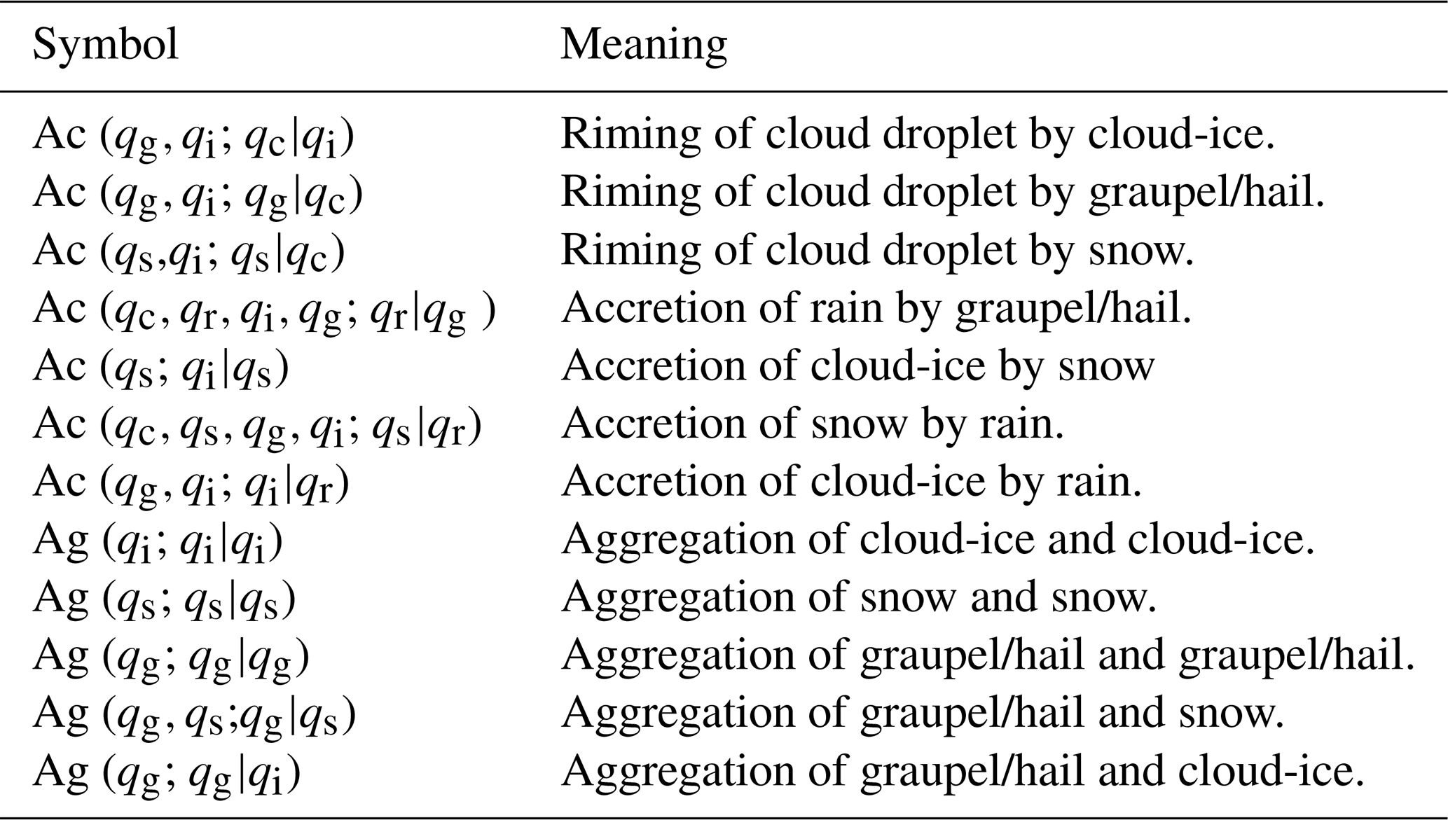
The emulated bin approach given in Sect. 2.2.4 is applied. For two species of interacting particles, x collecting y, the change in the mass mixing ratio per unit time is:

$$\begin{array}{}\text{(14)}& {\displaystyle \frac{\mathrm{\Delta }{q}_x}{\mathrm{\Delta }t}}=\sum _{i=\mathrm{1}}^{i=\mathrm{33}}\sum _{j=\mathrm{1}}^{j=\mathrm{33}}{\mathit{\chi }}_{x,y}(i,j)\mathrm{\Delta }{n}_x\left(i\right)\mathrm{\Delta }{n}_y\left(j\right)m_y\left(j\right)\end{array}$$

The corresponding change in the number mixing ratio is,

$$\begin{array}{}\text{(15)}& {\displaystyle \frac{\mathrm{\Delta }{n}_y}{\mathrm{\Delta }t}}=-\sum _{i=\mathrm{1}}^{i=\mathrm{33}}\sum _{j=\mathrm{1}}^{j=\mathrm{33}}{\mathit{\chi }}_{x,y}(i,j)\mathrm{\Delta }{n}_x\left(i\right)\mathrm{\Delta }{n}_y\left(j\right)\end{array}$$

i and j are the indices for discretised size bins. χ_x,y is the collection kernel. Δn_x(i) is the number mixing ratio of species x in ith size bin. Δn_y(j) and m_y(j) are the number and mass mixing ratios of y in jth size bin. More details for the calculations of the collection kernels are provided in Phillips et al. (2005, 2015).

Turbulent-induced enhancement of accretion is treated in the newly included processes using the approach by Benmoshe and Khain (2014). More details are provided in Kudzotsa et al. (2016).

3 Methodology for model validation with an observed case

3.1 Mid-latitude Continental Convective Clouds Experiment (MC3E) campaign

The MC3E campaign was carried out over the Atmospheric Radiation Measurement (ARM) Southern Great Plains (SGP) site in Oklahoma to study mesoscale convective systems (MCSs) from April to June 2011. The campaign consisted of a Central facility (CF) and 20 extended facilities, which covered an area with a 150 km radius. The campaign incorporated ground-based and in situ aircraft observations (Jensen et al., 2016).

3.1.1 Overview of observed storm on 11 May 2011

An MCS was initiated by a surface cold front with a parallel stratiform region north of a convective line (Jensen et al., 2016). The MCS storm consisting of this line of convective clouds was observed during 09:00 to 24:00 UTC on 11 May 2011. The storm had transitioned to a convective line with trailing stratiform cloud as it passed over the CF. The microphysical properties observed by aircraft were similar to those seen for trailing stratiform regions generally (Jensen et al., 2016).

3.1.2 Aircraft observations

Flights by the National Aeronautics and Space Administration (NASA) ER-2 and the University of North Dakota (UND) Cessna Citation 2 aircraft sampled the MCS between 18:00 and 21:00 UTC. The Citation carried probes to measure cloud microphysical properties.

Table 3 Instruments used to measure cloud properties carried on Citation 2 aircraft.

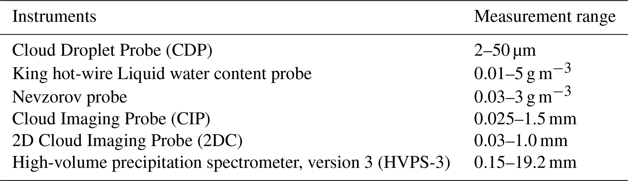
CDP measured the sizes and number concentration of cloud-droplets, and their liquid water content (LWC). 2DC, CIP and HVPS-3 measured the ice concentrations. The combined (“COMB”) spectrum includes the particle size distributions from 2DC (or CIP) and HVPS-3 probes. Shattering corrected tips were present for 2DC and HVPS-3 probes (Korolev et al., 2011) but not for the CIP. Following the method by Field et al. (2006) and Korolev et al. (2011), only ice crystals greater than 200 µm are considered for both observations and simulations in the validation plots.

3.1.3 Ground-based measurements

Xie et al. (2014) used control analysis to derive large-scale advective tendencies of heat and moisture and corresponding surface fluxes. These were applied to drive the simulations. Concentrations of active cloud condensation nuclei (CCN) were measured at seven supersaturation levels (Uin, 2016). The built-in SCAM nudging routine, which would tend to relax thermodynamic conditions to those observed, was not applied.

3.2 Model Setup

The observed case of the MCS was simulated from 10 to 13 May 2011 in SCAM6 with a global time step of 20 min and grid size of 100×100 km. Aerosol concentrations in each species are initially determined from the Goddard Chemistry Aerosol Radiation and Transport (GOCART) global model (Chin et al., 2000). These vertical profiles of aerosol concentration were then adjusted at all levels based on the averaged measurements near the ground from the Interagency Monitoring of Protected Visual Environments (IMPROVE) from 9 to 12 May 2011. More details of the initial aerosol conditions are provided in Waman et al. (2022).

4 Results from the control simulation with a new stratiform scheme

4.1  Validation of new scheme with observations

Simulations are performed with the new stratiform scheme referred to as “LS 24”. LS24 includes the new version of convection scheme (Jadav et al., 2025), for consistency in the treatment of microphysics. The predicted cloud hydrometer profiles are conditionally averaged over the simulation period and are validated against aircraft data. Regarding the aircraft observations, the stratiform region is considered to be where vertical velocity is less than 3 m s⁻¹. We also compare the results from the model simulation with the original convective and stratiform cloud schemes (the “MG08” run).

Figure 1a shows that the LS 24 run predicts the two precipitation peaks from deep convection at 21:00 UTC 10 May and 18:00 UTC 11 May with adequate timing, although the major convective peak is predicted about 6 h late for several reasons. First, the Zhang-McFarlane convection scheme in CAM6 uses a CAPE-based trigger with dilute CAPE closure. Previous studies have shown this tends to delay convection by 1–3 h in mid-latitude systems compared to convection-permitting models (Klein et al., 2009), and the same must be even more true in SCM simulations with no resolved 3D dynamics. Second, the VARANAL forcing dataset (Xie et al., 2014) represents domain-averaged conditions of large-scale advection into the simulated area (one global model grid-box), while the triggering processes in reality are sub-gridscal. Third, the forcing omits advection of condensate.

Moreover, both predicted peaks of precipitation rate (10 and 11 May) have insufficient intensity by a factor of 2 (weaker initial peak) and by about 20 % (main peak) respectively (Fig. 1a). The contributions from stratiform cloud are only minor during both predicted peaks. However, a consequence is that a surplus of humidity in the environment remains to allow too much deep stratiform cloud after the main peak on 12 May, especially during the subsequent 12 h. Then there is too much stratiform precipitation with weak peaks of 2 or 3 mm h⁻¹ (12 May), approaching intensities of both prior convective peaks (10 and 11 May) noted above. This stratiform precipitation on the final day (12 May) compares with practically none observed.

Regarding the cumulative surface precipitation (Fig. 1b), this is slightly over-predicted by only about 10 % at the end of the simulation for LS24, predicting 26.5 mm versus 24.0 mm observed. Stratiform precipitation overall contributes 65 % to the predicted accumulated precipitation with the LS24 run, in agreement with detailed simulations of the case by AC (Gupta et al., 2023). Thus, the bias noted above of stratiform precipitation on the final day (12 May), predicted but not observed, is explicable as a delay of about 12 to 15 h in the fall-out of most of the simulated stratiform precipitation, consistent with under-prediction of convective outflow of deep precipitating stratiform cloud. Whereas in nature, deep convection generates stratiform cloud by detrainment from cores in any MCS simultaneously, the model tends to generate the stratiform cloud from the environment independently (a similar decoupling problem is evident in the far weaker precipitation from MG08 in Fig. 1b). This is a cloud-dynamics bias that appears to be a feature of the treatment of convective outflow in CAM, unrelated to the microphysics. It is also possible that the mixed-phase stratiform cloud produces precipitation too slowly by the ice crystal process.

Table 4 shows that the LS24 run has an error of about 20 % to 30 % in the radiative fluxes at TOA and at the surface when compared to the satellite observations. An under-prediction by 17 % of net shortwave radiative flux at TOA entering the climate system is consistent with the model over-estimating the amount of cloud condensate in layer-cloud. This bias is consistent with that noted above of stratiform precipitation persisting for too long after the major convective peak on the final day. Similarly, insufficient outgoing longwave radiation at TOA by 20 % is explicable in terms of cold layer-cloud that is too high or similarly too extensive. It can be inferred from Fig. 3, a significant amount of ice crystals exists at upper levels because of homogeneous freezing. Higher-level clouds with abundant ice crystals act to reduce the longwave radiation emitted to space. Nevertheless, the radiation predictions are more accurate than for the MG08 scheme.

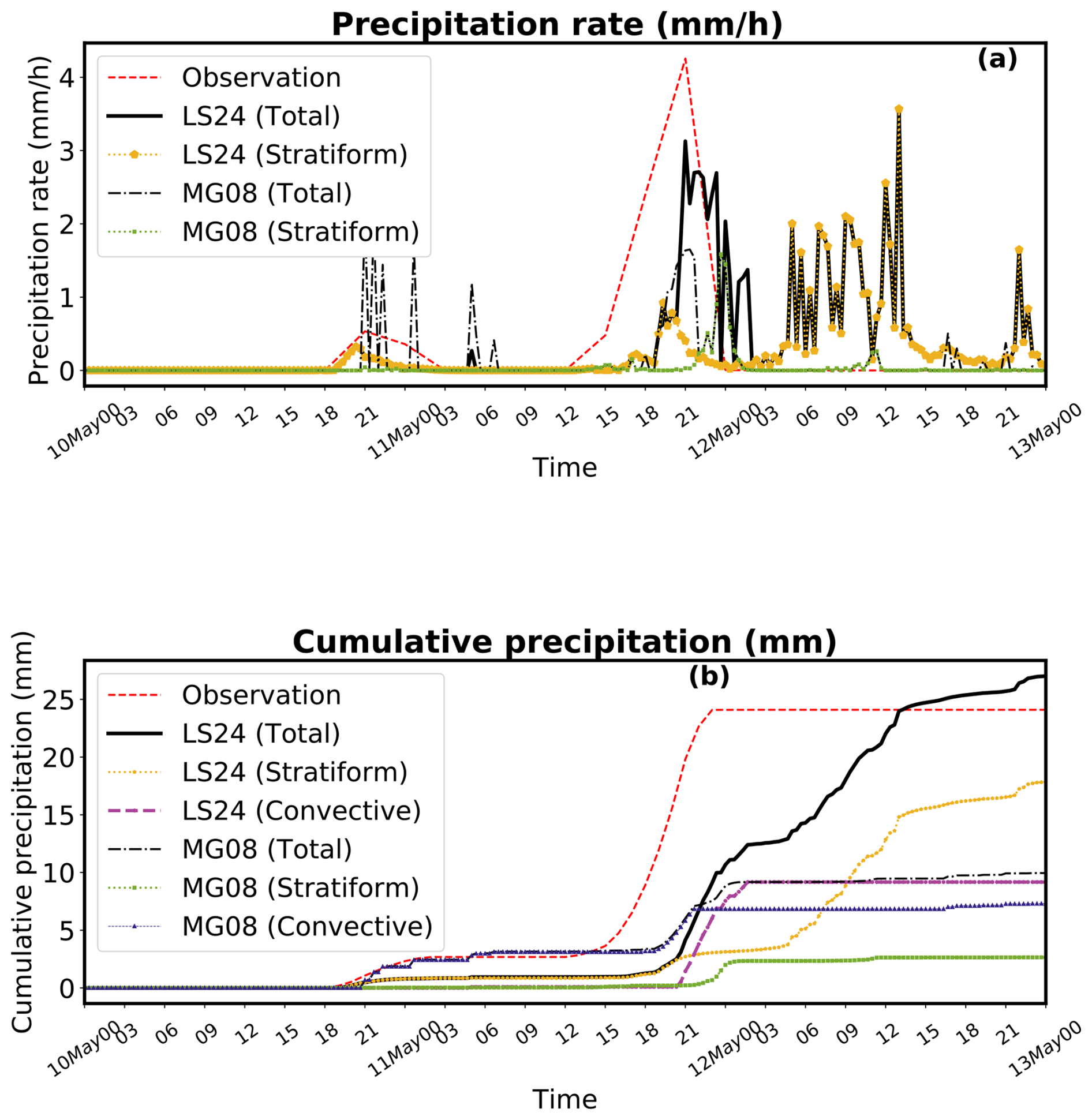
Figure 1 Comparison with MC3E observations of the domain-wide average predictions, from the original model, MG08 (dash-dotted black line), and the present modified scheme, namely LS24 (solid black line), of (a) precipitation rate (mm h⁻¹) and (b) cumulative surface precipitation (Xie et al., 2014).The average bias in (b) at the end of the simulation is +10 % for LS24 and −60 % for MG08. Also shown are the components of these predictions from stratiform precipitation (faint dotted lines).

Table 4 Unconditional average (evaluated regardless of clouds) of the radiative fluxes for the simulation period from 00:00 UTC 10 May 2011 to 00:00 UTC 13 May 2011.

Figure 2a shows that the LS24 run predicts the cloud base is at 16 °C, in agreement with detailed simulations by our high-resolution AC model (Waman et al., 2022). The LWC predicted by the LS24 run, agrees well with the aircraft observations and falls within the 90 % confidence intervals for mean values. The LS24 run predicts a maximum LWC of 0.5 g m⁻³ at 14 °C. The observed LWC data-points differ less from the LS24 simulation than they do from each other. The LS24 average bias is about 10 % and MG08 is +30 %.

Figure 2b shows the cloud droplet number concentration (CDNC) in comparison with the probe data (King, Nevzorov and CDP probes). CDNC predicted by the LS24 run agrees with aircraft observations at most levels. Both LS24 and MG08 have a similar average bias of about 10 %.

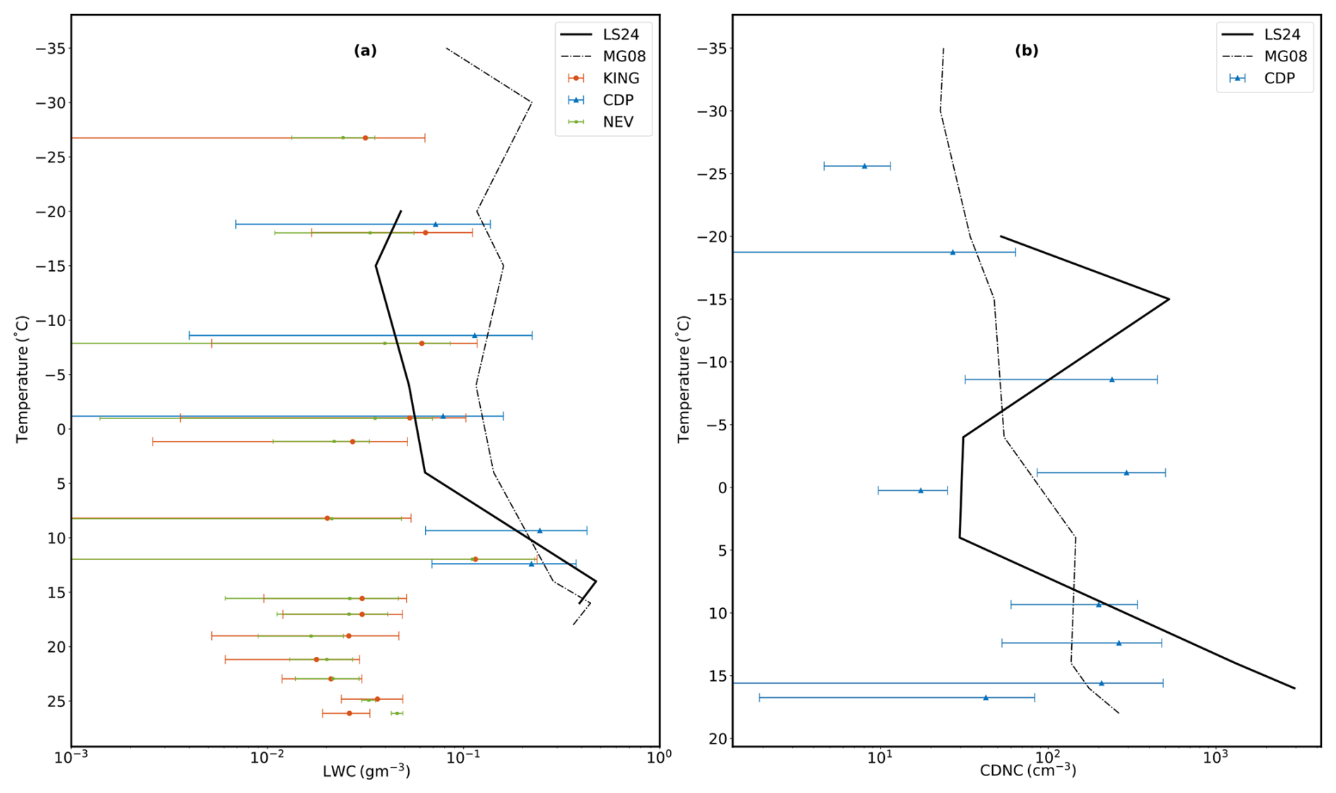
Figure 2 Predicted (a) liquid water content (g m⁻³) with CDP, King and Nevzorov probes, the average bias being about +10 % for LS24 and about +30 % for MG08 (b) cloud droplet number concentrations (cm⁻³) compared with observations from the CDP probe, from the MG08 (dashdotted black line with square) and LS24 (solid black line) simulations, the average bias being about 10.0 % for MG08 and LS24 Error bars shown are standard errors of observation samples. The cloud microphysical properties are conditionally averaged over the entire simulation period.

If left uncorrected, the artificial bias from ice shattering on the probe would increase the measured number concentrations of ice particles by an order of magnitude or more, especially at smaller sizes (Korolev et al., 2011). Therefore the observations were corrected with anti-shattering tips and by considering data only for sizes > 200 µm and 1 mm. The same size threshold is applied to the simulation results to be consistent.

Figure 3a shows agreement of the predicted average of ni₂₀₀ (ice number concentration of particles with sizes >200 µm) from LS24 with the aircraft observations, which vary logarithmically in the vertical. The predicted concentration of ice particles has the correct order of magnitude and differs from the observed values by less than the measurement error of the observations, with different probes at any given level differing from each other by almost an order of magnitude. Near the freezing level, ni₂₀₀ predicted by the LS24 run differs by only about 30 % from observations. LS24 average bias is −58 % and MG08 is −84.0 %. LS24 has a lower absolute bias.

Figure 3b shows that the prediction of ni₁ for precipitation (ice number concentration of particles >1 mm) from LS24 has the same order of magnitude as the aircraft observations in the lower half of the “mixed-phase region” of temperature (0 to about −36 °C). This is where both liquid water content (LWC > 0.01 g m⁻³) and ice water content (IWC > 0.01 g m⁻³) may co-exist. In the MC3E case, the mixed-phase region spans altitudes of 4–9 km (corresponding to −5 to −30 °C). It is where supercooled liquid droplets and ice particles may interact through either the Bergeron-Findeisen process, riming, and other microphysical processes. Although it is lower by an order of magnitude in the upper half, only one probe (HVPS) for the larger sizes is available and the instrumental error is difficult to quantify (Fig. 3b). If there is an uncertainty by an order of magnitude in the measurement of these concentrations, as noted above for the smaller sizes (>0.2 mm) in view of the spread among various probes, then there is little evidence of any bias with the larger sizes. the average bias is −86 % for LS24 and for MG08 is −95 %, so LS24 is more accurate by about half an order of magnitude. However, LS24's bias ranges from −55 % at very cold temperatures to +100 % at warm temperatures, representing bidirectional errors that partially cancel.

Figure 3c shows the ice water content (IWC) predicted by the LS24 run agrees with the observations at most levels, with the correct order of magnitude. However near the −20 °C level, the IWC is under-predicted by half an order of magnitude. Overall with the new scheme, the distribution of predicted IWC is much closer to the observations than is the MG08 scheme, as for the filtered ice concentrations noted above. The average bias is −32 % for LS24 and for MG08 is −66 %. LS24 demonstrates decisive superiority with a lower bias. Remarkably, LS24 achieves 0 % bias at −26 °C (perfect agreement at this optimal temperature) and maintains good performance through −11 °C (−18.2 % bias), with accuracy degrading only near 0 °C where mixed-phase conditions create measurement ambiguity. MG08 shows consistently poor performance across all temperatures (−65 % to −83 %), suggesting a fundamental calibration deficiency.

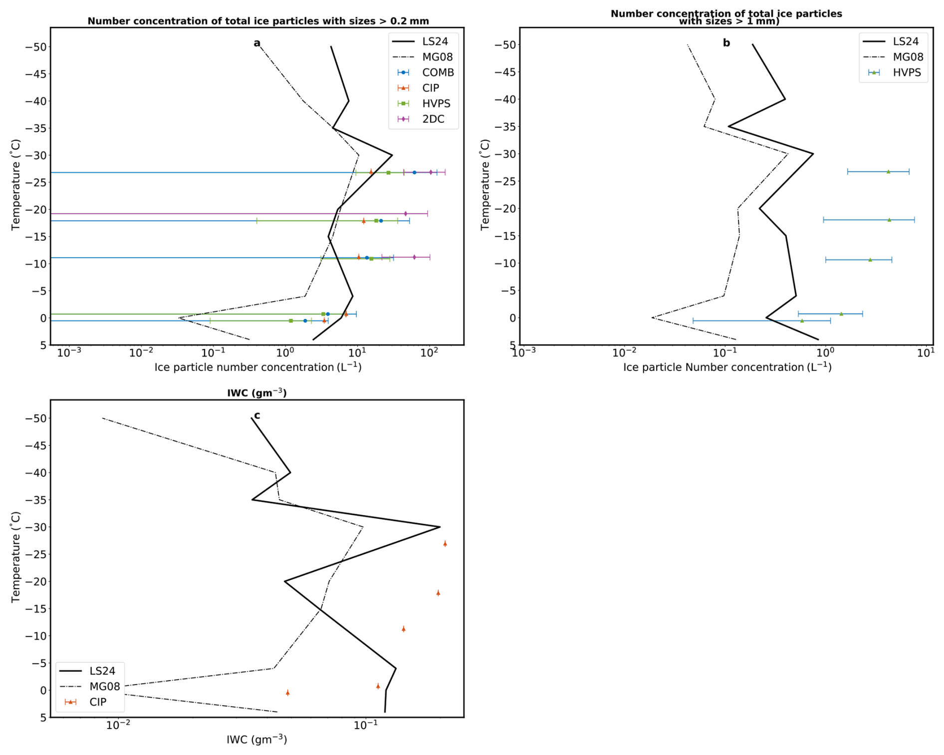
Figure 3 Predicted (a) concentration of ice particles with sizes >0.2 mm compared with observations from the 2DC, CIP, HVPS-3 probe and COMB, LS24 average bias is −58 % and MG08 is −84.0 %, normalized Root Mean Square Error (RMSE) for LS24 is 66 % and for MG08 is 97 % (b) ice number concentrations of all ice particles with size >1 mm compared with aircraft observations from the HVPS-3 probe, LS24 average bias is −86 % and MG08 is −95 %, normalized RMSE for LS24 is 103 % and for MG08 is 113 % and (c) total IWC from the MG08 (dashdotted black line with square) and LS24 (solid black line) simulations, LS24 average bias is −32 % and MG08 is −66 %, normalized RMSE for LS24 is 43 % and for MG08 is 65 %. Error bars shown are standard errors of observation samples.

4.2 Comparison between the MG08 and LS24 scheme

The MC3E storm was simulated with the original unmodified version of the model, and the run is referred to as the MG08 run. Accuracy of results is compared between the MG08 and LS24 runs.

The original SCAM6 model (MG08) predicts adequately the timing of the total precipitation peaks at the end of 10 and 11 May, but under-estimates the intensity of the second (main) peak. The first peak is predicted to be purely convective when according to the detailed simulation it was mostly stratiform (Gupta et al., 2023). The cumulative surface precipitation from MG08 is 60 % lower than observations by the end of the simulated period, which is much less accurate than that for LS24 noted above. Generally, only 30 % of all precipitation is stratiform for MG08, while detailed high-resolution simulations with AC, comprehensively validated by Gupta et al. (2023), show that this fraction is 80 %. Thus LS24 appears to agree better with observations in the cause and intensity of precipitation than does MG08.

Figure 2a shows the LWC predicted by both schemes does not differ so greatly, with a higher LWC from MG08 by up to a factor of 3 relative to the new scheme (LS24). LS24 is more in agreement with the aircraft observations, though MG08 is not inconsistent with these in view of the variability among the limited number of aircraft traverses. Figure 2b, shows that both runs (MG08, LS24) are similarly in agreement with the observations of CDNC at most levels.

Figure 3a shows that at all levels, ni₂₀₀ values predicted by both schemes mostly agree with the observations, though less so for MG08 than for the new scheme (LS24). Below the −10 °C level, the value from MG08 is up to an order of magnitude too low compared with the observations. Generally, the ice concentrations from MG08 are lower than from LS24 by up to an order of magnitude. Above the homogeneous freezing level (−36  °C), ni₂00 predicted by MG08 is up to an order magnitude lower than the LS24 run. Figure 3b shows that the precipitation concentration, ni₁, predicted by the MG08 run, is at least an order of magnitude lower than observations at all flight levels, being lower than LS24 by at least half an order of magnitude at most subzero levels.

Figure 3c shows that the original MG08 run under-predicts IWC by about half an order of magnitude throughout the mixed-phase region compared to observations. At most subzero levels, it is less than LS24 by up to an order of magnitude.

The MG08 run predicts net radiative fluxes slightly less accurately than the LS24 run. At the TOA the net shortwave and longwave fluxes are 30 % and 15 % too low respectively for MG08 compared to observations.

5 Results from Sensitivity tests

Table 5 List of the sensitivity simulations.

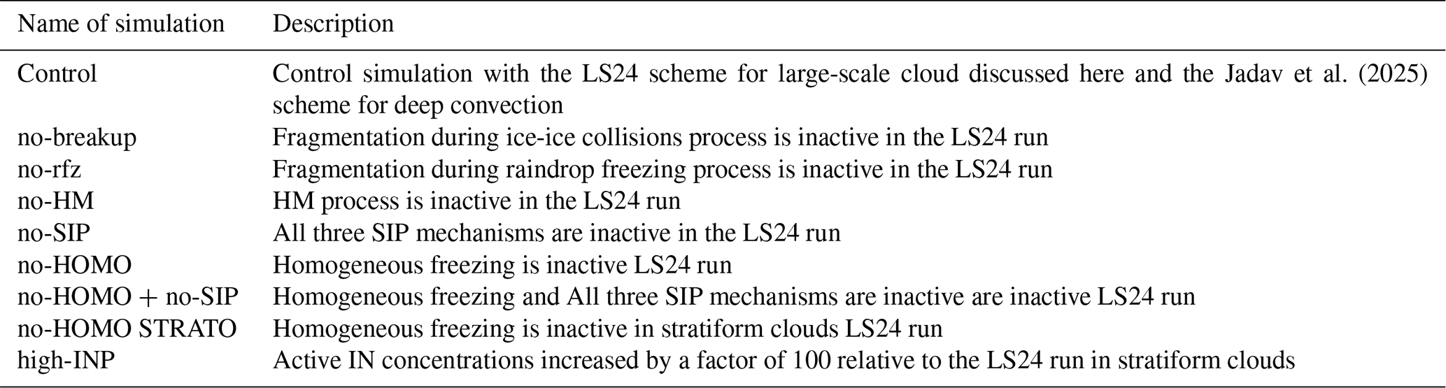
Sensitivity simulations were conducted to systematically examine the influence of different microphysical pathways of ice initiation and the role of environmental concentrations of active ice nuclei (IN) originating from solid aerosols such as mineral dust. Starting from the baseline LS24 run (Sect. 4.1), a suite of perturbation experiments was performed, each designed to isolate the effect of a specific microphysical or environmental modification. These included the following runs: (i) “no-breakup”, where the ice–ice collisional breakup process was prohibited; (ii) “no-rfz”, in which the rime-splintering process was switched off; (iii) “no-HM”, which removed all Hallett–Mossop ice multiplication effects; (iv) “no-SIP”, where secondary ice production by other pathways was switched off; (v) “no-HOMO”, where homogeneous freezing was deactivated; (vi) “no-HOMO + no-SIP”, excluding both homogeneous freezing and secondary ice production; (vii) “no-HOMO STRATO”, removing homogeneous freezing exclusively in the stratospheric layers; and (viii) “high-INP”, with elevated ambient concentrations of ice-nucleating particles to mimic enhanced dust loading. Comparison of these targeted perturbation simulations with the control run (LS24) allows for a detailed attribution of changes in cloud microphysics, radiative fluxes, and precipitation characteristics to specific ice initiation mechanisms and ice-nucleating aerosol conditions. Full descriptions of each configuration are provided in Table 5.

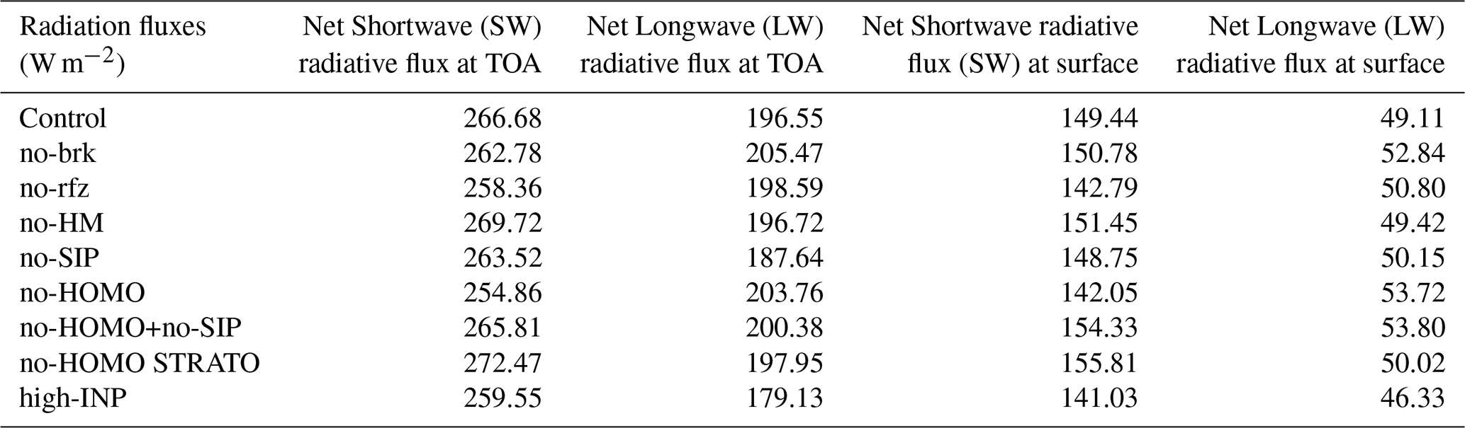
Table 6 Unconditional average of the radiative fluxes for the simulation period from 00:00 UTC 10 May 2011 to 00:00 UTC 13 May 2011 for the sensitivity simulations. Positive values of SW and LW flux signify radiations propagating downwards and upwards, respectively, into the climate system.

5.1 Ice initiation pathways

The simulations show the various sensitivities to different pathways of ice initiation. The mechanisms were prohibited as discussed in Table 5 in both the stratiform and convective microphysics schemes.

Figure 4 shows that excluding all SIP mechanisms (no-SIP case) produces relatively modest changes in ice water content and ice number concentration relative to the control run, with differences of 15 %–25 % rather than the order-of-magnitude changes sometimes reported in other studies. Prohibiting all SIP reduces the snow number concentration by up to a factor of two in the mixed phase region (Fig. 4c) relative to the control. Excluding breakup in ice-ice collisions reduces the snow number concentration by half an order of magnitude in the lower half of the mixed phase region. The corresponding changes in the snow mass content are minimal.

This muted sensitivity stems from several factors specific to the MC3E case and the model configuration. At temperatures below about −36 °C in cloud-top regions, homogeneous freezing produces explosive ice concentrations (10³ to 10⁴ L⁻¹) that swamp the SIP contribution. Figure 4a shows homogeneous freezing contributes about 99 % of the ice particle concentration at $T<-\mathrm{36}$ °C. Since most of the ice particles originate at upper levels where homogeneous freezing dominates and are downwelled, disabling SIP has limited impact on column-integrated IWC. Comparison with high-resolution simulations of the same case by Waman et al. (2022) reveals that the homogeneous ice is downwelled too far into the lower half of the mixed-phase region in the SCM runs, which tends to evaporate supercooled cloud-liquid. This artificially inhibits graupel production and SIP. Moreover, as noted above, too little production of deep stratiform cloud by convective outflow, as noted above (Sect. 4.1), would tend to mute the sensitivity with respect to SIP, which produces most of the ice in the convective cores (Jadav et al., 2025).

As noted above, Fig. 4a shows without homogeneous aerosol freezing in the large-scale clouds (no-HOMO STRATO case), the ice concentration is reduced by two orders of magnitude in the mixed phase region of temperature (0 to −36 °C) and by even more aloft in cirriform clouds. Further removal of all other homogeneous freezing causes only a slight reduction by up to 30 % relative to the no-HOMO STRATO case. Regarding SIP, the no-SIP run reveals little systematic impact on stratiform ice concentration from all SIP in the control run, which is explicable in terms of the prevalence of homogeneous ice throughout all sub-zero levels. Switching off individually each SIP mechanism perturbs the ice concentration by up to ±50 %, due to alteration of precipitation amounts aloft and supercooled cloud liquid properties, affecting homogeneous freezing in a non-linear way.

Figure 4b shows a marked reduction of IWC by about an order of magnitude in the upper half of the mixed-phase region when homogeneous aerosol freezing in the large scale cloud scheme is prohibited. There is a similar reduction in the cirriform cloud at upper levels. This is all consistent with the decrease in ice number concentration noted above. The complete removal of all other homogeneous freezing (no-HOMO) further decreases IWC slightly (by 20 %) relative to no-HOMO STRATO, with a comparatively small incremental change. The no-SIP run results in minor changes to the IWC profile relative to the control, reaffirming the dominance of homogeneous freezing in driving ice mass in the simulations. Switching off individual SIP processes introduces variations in IWC of up to ±40 %, attributed to their perturbation of mixed-phase cloud microphysics, especially through indirect effects on alterations of vapor growth, riming, and sedimentation of ice.

Figure 5a and b show how the cloud liquid properties are influenced by SIP mechanisms and homogeneous freezing. The no-SIP run shows an increase in the supercooled LWC throughout the mixed phase region by 10 % relative to the control, because the growth of fewer ice particles causes less depletion of liquid by evaporation and riming. For similar reasons, in the lower half of the mixed phase region of the cloud, prohibiting all homogeneous freezing boosts the LWC by about half an order of magnitude relative to the control. The cloud droplet number concentration is mostly increased by excluding either homogeneous freezing or SIP, because the descent of homogeneous ice into the mixed-phase region creates more subsaturation with respect to water, evaporating supercooled cloud-liquid.

Figure 5c,d shows that the mass and number concentrations of rain are perturbed but not in a systematic manner at all levels by the exclusion of most of the mechanisms of SIP and homogeneous freezing. An exception to this is the exclusion of breakup in ice-ice collisions, which reduces the rain concentration by about an order of magnitude below the freezing level and by about half an order of magnitude above. Yet there is much less impact from excluding all SIP processes, indicating cancellation among these. Another exception is exclusion of all homogeneous freezing, which boosts the supercooled rain concentration by half an order of magnitude in the lower half of the mixed-phase region, due to the impact on supercooled LWC noted above.

Figure 6a, b shows that the two major convective peaks seen in the observations (10 May, 21:00 and 11 May, 21:00) are predicted to be boosted by about 20 % from the SIP being prohibited, but the stratiform precipitation following the major peak on the final day is slightly weakened (by 20 %). Switching off all the homogeneous freezing drastically weakened the stratiform precipitation on the final day by a factor of about 2, similarly diminishing the cumulative surface precipitation. The no-breakup case run had a cumulative surface precipitation very similar to the no-SIP run, indicating that the breakup in ice-ice collisions dominates the overall SIP impact on precipitation.

Figure 6c, d shows the impact on the top of the atmosphere radiation, also detailed in Table 6. The no-SIP run has a TOA Net Shortwave flux entering the atmospheric column that is 3 W m⁻² lower than control due to more cloud condensate aloft at sub-zero levels with a corresponding reduction in the outgoing long-range radiation, relative to control. Without homogeneous freezing, there is a stronger reduction (by 12 W m⁻²) in SW flux entering the climate system than without SIP due to more cloud condensate aloft. However, at upper levels there is less homogeneous ice and more emission of longwave radiation to space from warmer average emitting level when homogeneous freezing is excluded.

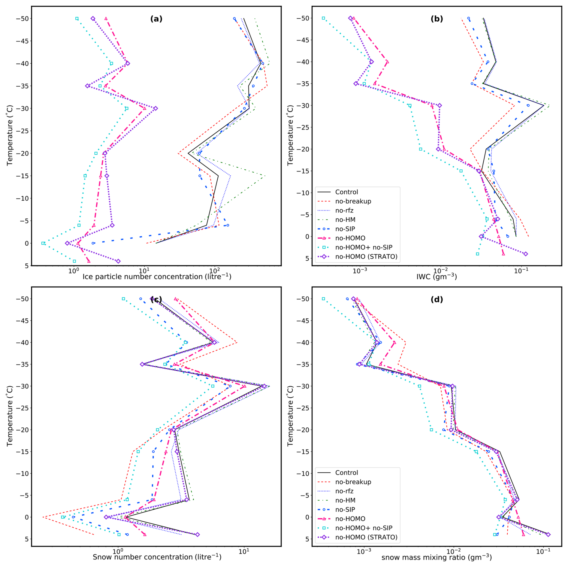
Figure 4 Predicted (a) Ice particle number concentration (L⁻¹), (b) IWC (g m⁻³), (c) Snow number concentration (L⁻¹), (d) Snow mass content (g m⁻³). The cloud microphysical properties are conditionally averaged (over stratiform cloud regions only) over the entire simulation period.

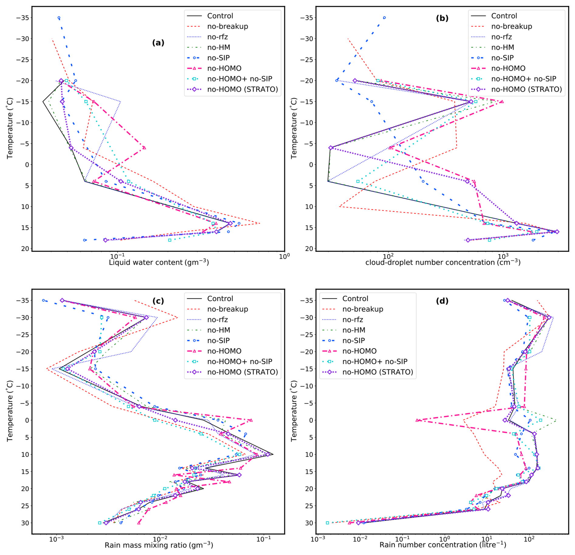
Figure 5 Predicted (a) Liquid Water Content (g m⁻³), (b) cloud droplet concentration, CDNC (g cm⁻³), (c) Ice water content (g m⁻³), (d) CDNC (cm⁻³), (c) rain mass mixing ratio, (d) rain number concentrations (L⁻¹). The cloud microphysical properties are conditionally averaged (over stratiform cloud regions only) over the entire simulation period.

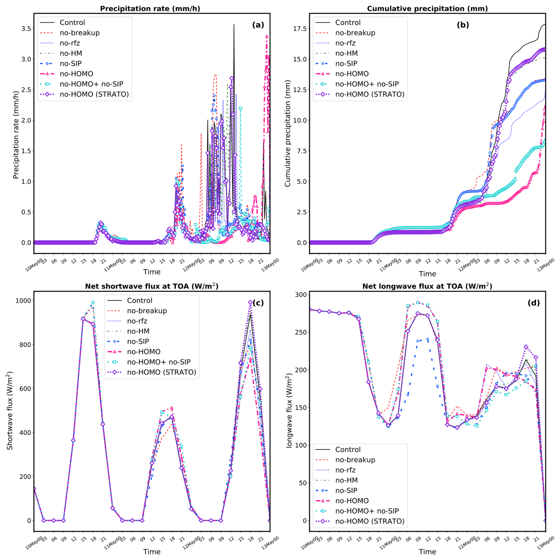
Figure 6 Predicted (a) surface precipitation rate (mm h⁻¹), (b) accummulated surface precipitation (mm), (c) net shortwave flux at TOA (W m⁻², positive downward), and (d) net longwave flux at TOA (W m⁻², positive upward). In (a) and (b), only the stratiform components of precipitation are shown.

5.2 Environmental aerosol conditions affecting ice nucleation

Figure 7a illustrates the response of ice number concentration in the sensitivity experiment where the concentration of ice nucleating particles (INPs) in the environmental aerosol population is increased by a factor of 100 at all levels. Despite already high baseline loadings of INPs, the Figure reveals that the ice number concentration exhibits more than an order-of-magnitude variation across the temperature range. In the control simulation at subzero levels, homogeneous freezing is the dominant mechanism for ice formation overall, since it occurs at temperatures colder than about −36 °C, and humidities approaching water saturation (high supersaturations with respect to ice). This leads to a high number of ice crystals aloft at upper levels which are then downwelled somehow.

In contrast, the high-INP case (100× INP numbers) activates heterogeneous nucleation more intensely during (e.g., large-scale) stratiform ascent – at warmer temperatures and lower supersaturation. This early onset of ice formation limits the buildup of supersaturation necessary for homogeneous freezing, thereby suppressing it. As a result, the homogeneous nucleation pathway and the related downwelling of very numerous ice particles are effectively “switched off” in the high-INP case, leading to an overall reduction in total ice number concentration throughout the mixed-phase region of temperature, as is evident in Fig. 7. Thus, the model represents the known competition between homogeneous aerosol freezing and heterogeneous ice nucleation in cirriform clouds (Kärcher and Lohmann, 2002). The early consumption of water vapor by heterogeneous nucleation prevents further crystal formation homogeneously and shifts the microphysical regime.

Moreover, with fewer ice crystals forming overall in the high-INP case, the competition for water vapor during growth is reduced. This enables existing crystals to grow larger, contributing to increased snow production. The enhanced snow growth can lead to greater meltwater generation and subsequently more rainfall through the ice crystal process of precipitation (or “cold-rain process”), consistent with findings reported by Gupta et al. (2023). Finally, Fig. 7 also reflects a shift in the equilibrium saturation conditions – ice formation occurs at a lower saturation threshold in the high-INP scenario

Figure 7b shows that the ice water content (IWC, g m⁻³) follows a pattern consistent with the response of ice number concentration to increased INP loadings under the 100× INP sensitivity scenario. In the control simulation, where homogeneous freezing dominates at lower temperatures and high supersaturation, the rapid formation of numerous ice crystals leads to elevated IWC values. In contrast, in the high-INP case, earlier initiation of heterogeneous nucleation results in fewer crystals forming, thereby lowering IWC in regions that would otherwise favor homogeneous freezing. However, the larger size of ice particles in the high-INP case noted above partially compensates and maintains moderate IWC values across a portion of the temperature range. This balance between fewer but larger crystals shapes the overall IWC response and underlines a shift in the ice growth regime.

Figure 7c also illustrates the snow number concentration (L⁻¹), providing insight into how ice particles evolve into precipitation-sized snow. In the control case, where homogeneous nucleation yields a high number of small ice crystals, subsequent growth processes (e.g., riming and aggregation) produce a relatively large number of snow particles. In the high-INP simulation, however, the fewer initial crystals noted above cause the downstream formation of snow particles, leading to lower snow number concentrations. The reduced competition for water vapor, and the greater abundance of supercooled cloud-liquid from fewer crystals in the large-scale cloud (Fig. 8), in this scenario favors the growth of fewer, but larger, snow particles. This further highlights the shift in microphysical pathways due to increased INP concentrations.

The snow mass content (g m⁻³) in Fig. 7d shows that, while the snow number concentration is reduced in the high-INP scenario relative to the control, the snow mass content does not decline proportionally. This is because the reduced number of snow particles grow more efficiently, reaching larger sizes as with the ice crystals. In some temperature regimes, the snow mass mixing ratio is even enhanced relative to the control case, signifying more efficient precipitation development. This outcome supports the interpretation that the high-INP regime promotes a shift toward fewer but more massive snow particles, enhancing cold-rain production from melting of ice precipitation (Fig. 8), in line with the findings of Gupta et al. (2023).

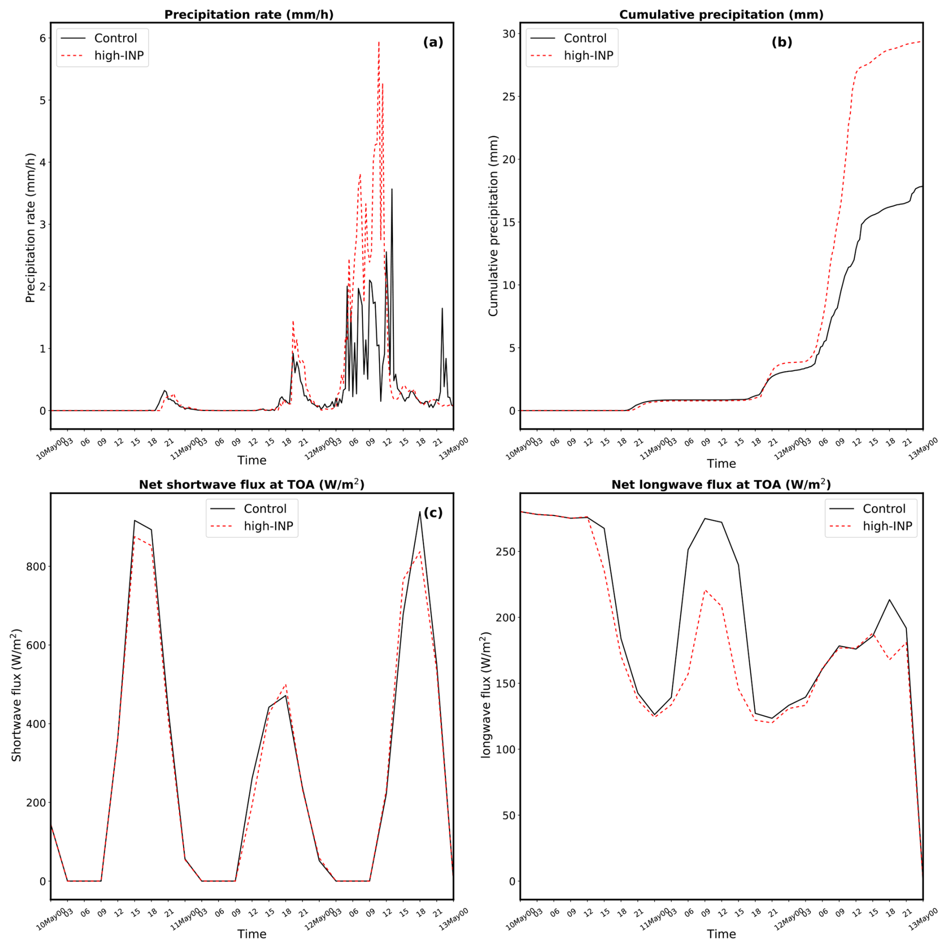
Figure 9a shows that in the control case, where homogeneous nucleation dominates, surface precipitation occurs in intermittent bursts with moderate peak intensities. By contrast, the high-INP case has more frequent and stronger peaks in surface precipitation rate. This outcome arises from earlier activation of heterogeneous nucleation, which limits homogeneous ice formation but favors the rapid growth of fewer ice crystals into precipitation-sized hydrometeors. The cumulative precipitation (mm) in Fig. 9b further highlights this difference. Both simulations initiate precipitation at nearly the same time, yet the high-INP case produces considerably more accumulated surface precipitation. This is consistent with a microphysical regime where fewer but larger ice and snow particles grow more efficiently, ultimately enhancing cold-rain production through melting, as also noted in Gupta et al. (2023). Figure 9c–d show the radiative implications of these changes at the top of the atmosphere (TOA). The net shortwave flux (Fig. 9c) is slightly reduced in the high-INP case, reflecting enhanced cloud shading due to more persistent condensate and precipitation. Meanwhile, the net longwave flux (Fig. 9d) reveals systematically lower outgoing fluxes at TOA for the high-INP simulation, consistent with deeper, longer-lived cloud layers that trap infrared radiation, partially re-emitting it at a colder temperature aloft to space. Taken together, Fig. 9 demonstrates that the increase in INP concentrations not only modifies the microphysical pathways of ice initiation – shifting from homogeneous to heterogeneous nucleation – but also amplifies precipitation production and alters the radiation budget at the TOA.

In summary, the higher numbers of INPs act to shift the dominant pathway of ice initiation from homogeneous to heterogeneous ice nucleation in the simulations, as expected. This occurs by their effect on lowering the humidity aloft. Such changes in nucleation pathways not only influence the number of hydrometeors but also their mass, with significant implications for precipitation.

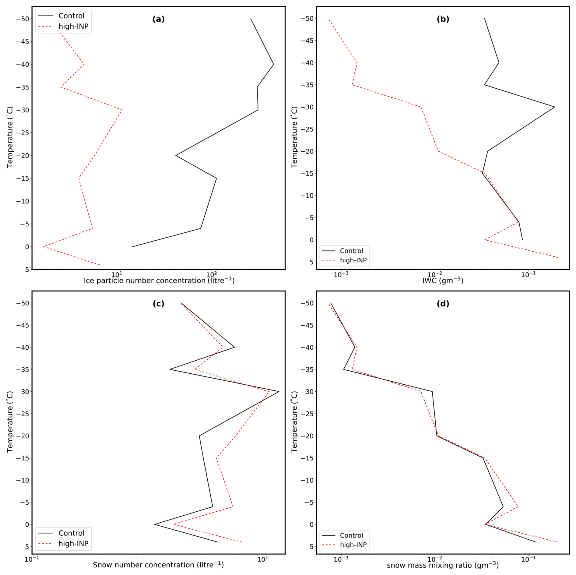
Figure 7 Predicted (a) ice particle number concentration (L⁻¹), (b) IWC (g m⁻³), (c) snow number concentration (L⁻¹), and (d) snow mass content (g m⁻³). The cloud microphysical properties are conditionally averaged (over stratiform cloud regions only) over the entire simulation period.

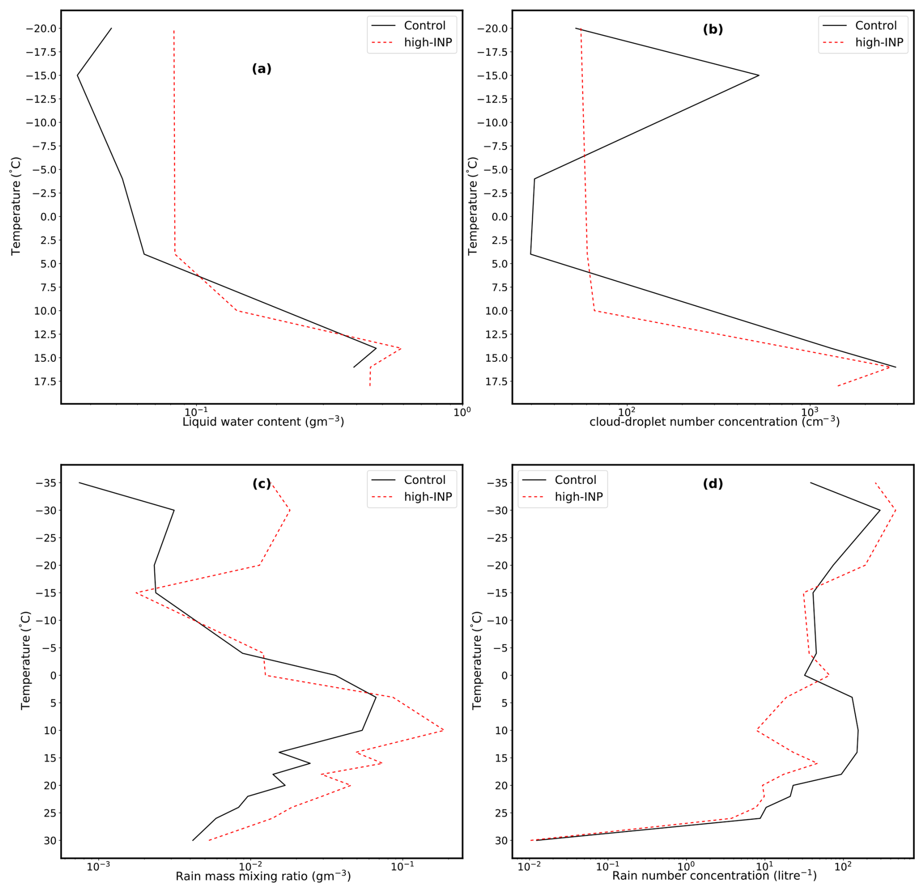
Figure 8 Predictions from the high-INP case for (a) liquid water content (g m⁻³), (b) cloud droplet concentration, CDNC (cm⁻³), (c) rain mass content (g m⁻³), and (d) rain number concentrations (L⁻¹). The cloud microphysical properties are conditionally averaged (over stratiform cloud regions only) over the entire simulation period.

Figure 9 Prediction of surface stratiform precipitation and radiative fluxes at TOA for the high-INP case, plotted as in Fig. 6.

6 Conclusions

In this study, the large-scale cloud microphysics scheme MG08 has been substantially modified through the introduction of physically-based representations for key microphysical processes, as described in Sect. 2.2. This updated scheme – referred to as LS 24 – was implemented within SCAM6 and used to simulate the MC3E storm, with a focus on understanding the role of homogeneous nucleation and secondary ice production (SIP) mechanisms in shaping mixed-phase cloud microphysics and associated storm properties.

Key conclusions are as follows:

• 1.

  The new scheme improves the accuracy of the prediction for the control run of the MC3E storm:

  • –

    There is a 10 % slight over-prediction of cumulative surface precipitation over the entire simulationm with the new scheme, compared with an under-prediction by 60 % with the original scheme by MG08. Moreover, the surface precipitation is predicted for the right macrophysical reasons, with 65 % coming from stratiform precipitation compared with 30 % for the original scheme over the entire simulated period. The corresponding fraction is about 80 % from our detailed high-resolution simulations (AC) (Gupta et al., 2023).

  • –

    Predictions of concentrations of ice concentrations and related supercooled LWC are also improved, with the correct order of magnitude of total ice (> 0.2 mm) concentrations being predicted (half an order of magnitude more accurate than MG08).

  • –

    Prediction of SW radiative fluxes at TOA and surface are improved (low bias at TOA reduced from about 30 % to 20 %) due to reduction of the over-estimate of cloud condensate amount aloft. Little improvement occurs in the LW fluxes, however.

• 2.

  In the control run, supercooled cloud droplets in stratiform clouds are largely depleted through accretion onto rain and ice rather than undergoing homogeneous freezing. Sensitivity experiments (Fig. 4a, compare crimson and purple lines) confirm that in the control simulation the homogeneous freezing of solute aerosols, rather than supercooled cloud-droplets, plays a dominant role in controlling ice number concentrations in large-scale regions at most subzero levels. Homogeneous aerosol freezing occurs when the humidity approaches water saturation, and prevails in large-scale weak (stratiform$/$cirriform) ascent (e.g. Phillips et al., 2007), as expected from high-resolution cloud simulations (Phillips et al., 2007). In the simulation, this homogeneous ice is downwelled through the mixed-phase region, albeit arguably too far down (cf. Waman et al., 2022).

• 3.

  Prohibiting homogeneous freezing of solute aerosols in the large-scale (stratiform/cirriform) cloud regime leads to a reduction by up to two orders of magnitude in ice number concentration, especially within the mixed-phase region of temperature (0 to −36 °C). This also significantly reduces the IWC, with further suppression when all homogeneous pathways are disabled. SIP processes, while not dominant in this regime, contribute up to ±50 % variations in ice concentration and IWC through their nonlinear interactions with cloud liquid and precipitation processes.

• 4.

  Increasing environmental concentrations of active INPs by a factor of 100 triggers earlier heterogeneous nucleation during ascent, which inhibits the buildup of supersaturation required for homogeneous freezing. This transition reduces total ice and snow number concentrations but allows larger ice particles to form due to reduced vapor competition and more supercooled cloud-liquid for riming. The resulting microphysical shift enhances snow mass mixing ratios and is consistent with an increased cold-rain process.

• 5.

  Radiative impacts are also significant: sensitivity tests prohibiting either homogeneous freezing or SIP show reductions in both shortwave (net incoming) and longwave (outgoing) net radiative fluxes at the top of the atmosphere (TOA) due to more cloud condensate aloft and increased upper-level cold hydrometeors. These findings demonstrate the strong feedback between microphysical pathways and cloud-radiative interactions.

Regarding point 1 here, the updated LS24 scheme improves SCAM6's ability to represent stratiform cloud microphysics. Notably, the improved number concentrations of small- (>0.2 mm) and large-(>1 mm) ice particles in the stratiform cloud leads to a more realistic stratiform-to-convective precipitation ratio. This aligns better with observations and addresses known biases, such as the historical ∼ 70 % underestimation of stratiform precipitation in SCAM simulations. Consistent with Gupta et al. (2023), who found that about 80 % of surface precipitation during the MC3E storm came from stratiform clouds, our results confirm the critical importance of accurately representing ice initiation mechanisms in large-scale clouds to capture precipitation and cloud radiative effects.

However, the lack of sensitivity of the properties of stratiform cloud with respect to inclusion of homogeneously nucleated ice in convective cores (compare crimson and purple lines on Fig. 4a, b) calls into question the realism of the treatment of convective outflow. In both MG08 and LS24 runs, the peaks of surface precipitation from the stratiform cloud seem somewhat decoupled from the major peak of convective precipitation, when in reality they both occurred together over a 12 h period, as predicted by the high-resolution runs of this case (Gupta et al., 2023, their Fig. 3i, j). In principle, the treatment of convective detrainment would be expected to have been improved in LS24 due to the proven realism of the newly predicted microphysical properties in convective cores introduced by Jadav et al. (2025), which allow for more realistic prediction of cloud water/ice content and droplet/crystal number concentrations in any detraining outflow. However, the convective outflow is having little effect on stratiform properties. Future model development may focus on this apparent bias. Another limitation of the present study is the fact that only a single case has been simulated. In nature, different regimes of aerosol loading and of thermodynamic conditions such as convective instability would be expected to influence the cloud-type and hence the balance of initiation pathways for ice crystals, droplets and precipitation (e.g. Gupta et al., 2023). Future model development may also extend the validation testing to additional cases.

To conclude, the sensitivity of the storm system to aerosol loading is nonlinear and complex. Aerosol-induced changes to the environmental INP levels significantly modulate the formation, growth, and sedimentation of ice-phase hydrometeors by altering the balance between heterogeneous and homogeneous nucleation. These changes ultimately impact precipitation formation pathways, cloud longevity, and radiation budgets. The present paper shows that conventional global models with upgraded treatment of cloud microphysics can capture much of this complexity in the aerosol-cloud linkage.

Appendix A

Table A1 List of Symbols.