Beyond discrete stratocumulus regimes: a ternary continuum of morphology reveals within-regime variability in cloud susceptibilities

We introduce a new framework for defining marine stratocumulus cloud morphologies using a ternary diagram. A ternary diagram is a triangular representation of three components, with each vertex corresponding to 100 % of one component, and any point within the triangle representing a mixture of all three that sums to 100 %. We use cloud optical thickness (τ_c) as the diagnostic physical variable and accordingly define three corresponding τ_c classes. Different combinations of the three τ_c classes define different cloud morphologies, which vary continuously within the ternary space. The method is applied to one year of satellite observations of stratocumulus clouds and reveals the frequency of occurrence of the different morphologies across the ternary space. Large-eddy simulations complement the satellite analysis and show that cloud evolution tends to follow preferred paths across the ternary morphology space, explaining why the observations are concentrated within a limited range of morphologies. We further investigate the susceptibility of cloud liquid water path (LWP), cloud albedo, and cloud fraction to variations in droplet number concentration, conditioned on cloud morphology. We find that susceptibilities vary strongly with cloud morphology, yet in the most frequently occurring scenes, LWP and cloud albedo susceptibilities largely offset each other, resulting in a near-zero global in-cloud albedo response. We also find that cloud fraction susceptibility can be negative in low-LWP morphologies, presumably due to strong negative LWP adjustments. These findings have important implications for marine cloud brightening, whose effectiveness needs to be evaluated in a morphology-dependent framework to achieve the intended outcomes.

1 Introduction

Cloud albedo (A_c) is mainly determined by the liquid water path (LWP) and cloud droplet size. To first order these two properties set the cloud optical thickness (τ_c), which is the primary quantity controlling A_c. Aerosols can influence both LWP and droplet size, and thus A_c: An increase in aerosol concentration can raise the cloud droplet concentration (N_d), which reduces droplet size, given no change in cloud water (Twomey, 1974). This leads to an increase in A_c through a well-established physical mechanism (Platnick and Twomey, 1994; Twomey, 1974). This sensitivity of A_c to N_d is termed the cloud albedo susceptibility, $S_{A_{\mathrm{c}}}$. An increase in N_d can also initiate processes that influence the cloud water, which in turn also changes A_c (Ackerman et al., 2004; Albrecht, 1989; Bretherton et al., 2007). This latter effect, the LWP susceptibility to N_d, S_LWP, is termed LWP adjustment. Its sign and magnitude remain uncertain due to the complexity of the underlying processes (Glassmeier et al., 2021; Bellouin et al., 2020; Forster et al., 2021; Toll et al., 2019; Goren et al., 2025). Positive LWP adjustments amplify the cloud albedo response to N_d, whereas negative LWP adjustments counteract it. The combined effects of the cloud albedo response and LWP adjustments to changes in N_d determine the net in-cloud albedo susceptibility, S_net, which is the quantity that matters for the radiation budget of the Earth.

Cloud albedo varies spatially from meter scales up to hundreds of kilometers (Davis et al., 1997; Rampal and Davies, 2020; Stevens et al., 2020; Wood, 2006; Zhou et al., 2021). These spatial variations manifest as different cloud morphologies (Goren et al., 2023; McCoy et al., 2017; Eastman et al., 2024; Wood and Hartmann, 2006; Choudhury and Goren, 2024). Studies that classify stratocumulus cloud morphologies typically define discrete morphology regimes such as open cells, closed cells, and disorganized mesoscale cellular convection (Wood and Hartmann, 2006; Muhlbauer et al., 2014; Erfani and Hosseinpour, 2025; Wu et al., 2025; Yuan et al., 2020; Geiss et al., 2024). Nevertheless, there is a continuum of morphologies between these discrete regime definitions (McCoy et al., 2023; Choudhury and Goren, 2024; Goren et al., 2023), and even fully overcast closed cells, which are typically classified as a single morphology regime, can exhibit structural differences, for example with cells having different horizontal scales (Zhou and Feingold, 2023).

Most studies examine the dependence of cloud susceptibilities on cloud morphology by separating data into cloud scenes associated with different meteorological conditions or precipitation states. These factors co-vary with cloud morphology, which is typically defined by cloud fraction (CF) regime (Gryspeerdt and Stier, 2012; Gryspeerdt et al., 2019; Chen et al., 2025; Hoffmann et al., 2024, 2025; Toll et al., 2019; Glassmeier et al., 2021; Rosenfeld et al., 2019; Zhang et al., 2022). Nevertheless, even within the same type of CF regime, LWP and τ_c may still exhibit spatial variability, for example due to variations in veil cloud extent in open cells or in cell size distribution within closed cells (Goren et al., 2023; Wood et al., 2018; Zhou and Feingold, 2023). These variations can affect the derived susceptibilities, as shown by Goren et al. (2023) and Zhou and Feingold (2023). Zhou and Feingold (2023), for example, showed that S_LWP in closed cells with smaller horizontal extent can be up to ten times larger than in cells with larger horizontal extent. They attributed these differences to dynamically stronger entrainment-driven evaporation in the smaller cells. Also $S_{A_{\mathrm{c}}}$ has been shown to depend on morphology, as demonstrated by Goren et al. (2023), who found that $S_{A_{\mathrm{c}}}$ can be positively biased by up to 50 % if the spatial distribution of τ_c within a given 1°×1° scene is ignored.

Here, we introduce a new method for characterizing cloud morphology that provides a continuous, rather than a discrete, classification. Using this framework, we explore fundamental properties of marine low-level cloud morphologies and calculate cloud albedo, LWP, and CF susceptibilities to N_d conditioned on morphology. Section 2 introduces the ternary morphology approach, Sect. 3 presents the results, and conclusions are given in Sect. 4.

2 Data and methods

2.1 Data

Satellite observations of marine low-level clouds over the oceans between 60° N–60° S in 2015 were selected for the analysis. The observations were taken from the Moderate Resolution Imaging Spectroradiometer (MODIS) Aqua instrument (Platnick et al., 2016), which provides a nadir resolution of 1 km×1 km. Scenes were filtered to retain only single layer liquid clouds using the MODIS multilayer flag and cloud phase retrieval. Pixels with sensor zenith angles >55° or solar zenith angles >65° were excluded due to retrieval uncertainties (Grosvenor et al., 2018). The satellite retrieved variables used include the corrected reflectance at 0.86 µm, CF (at 5 km×5 km resolution), LWP, τ_c, and cloud top effective radius, r_e. N_d was derived from r_e and τ_c following Grosvenor et al. (2018). The cloud-core LWP was also computed, defined as the mean LWP of the 10 % of pixels with the highest LWP within a scene.

To diagnose cloud morphology, one must define an area large enough to capture the relevant morphological scales. For marine low level clouds, morphology scales range from a few tens of kilometers up to about 200 km (Zhou et al., 2021). Following this, the cloud properties of the filtered scenes were gridded onto a uniform 2°×2° latitude–longitude grid, selected to avoid sampling areas too small to represent the mesoscale cloud morphology. Only scenes with CF>40 % were used in the analysis to avoid broken cloud regimes with their attendant retrieval uncertainties (Choudhury and Goren, 2025; Grosvenor et al., 2018; Wolters et al., 2010). This criterion removes broken cloud regimes with low CF, such as shallow cumulus, sugar, and gravel (Stevens et al., 2020). Figure A1 shows the occurrence of the scenes included in the analysis, which are accordingly found mainly in the stratocumulus regions where closed cells, open cells, and other types of mesoscale cellular convection are common and have relatively higher CF (Muhlbauer et al., 2014). A_c was calculated following the approach of Schneider and Dickinson (1976):

$$\begin{array}{}\text{(1)}& {\displaystyle }{\displaystyle }{A}_{\mathrm{c}}={\displaystyle \frac{A_{\text{all-sky}}-A_{\text{clear-sky}}(\mathrm{1}-\text{CF})}{\text{CF}}}\end{array}$$

where A_all-sky and A_clear-sky were obtained from the Clouds and the Earth's Radiant Energy System (CERES) aboard Aqua (Loeb et al., 2005), and gridded to 2°×2° to match the gridded MODIS data. CF was obtained from MODIS Aqua (Platnick et al., 2016).

Large eddy simulation (LES) output was taken from Goren et al. (2019). The simulations were performed with the System for Atmospheric Modeling (SAM) LES model (Khairoutdinov and Randall, 2003) and were designed to represent a closed-to-open cell transition event observed over the northeast Atlantic Ocean. A full description of the model setup and the simulated case is provided in Goren et al. (2019).

2.2 Methods

2.2.1 Ternary diagram

A ternary diagram is a triangular graph used to visualize the proportions of three components in a mixture, where each corner of the triangle represents 100 % of one component and any point inside represents the relative contributions of all three, which must sum to 100 %. In this study, the three components are the percentages of cloudy pixels in three τ_c classes: thin (τ_c<7), intermediate ($\mathrm{7}\le {\mathit{\tau }}_{\mathrm{c}}<\mathrm{12}$), and thick (τ_c≥12). The partitioning of τ_c among the three components was done by counting the pixels in each 2°×2° scene whose retrieved τ_c falls into each of the three classes, then normalizing by the total number of pixels with a valid τ_c in the entire scene. Each scene can therefore be represented as a single point in the ternary diagram corresponding to a unique fractional composition of τ_c, which exhibits a unique morphology (see examples in Fig. 1).

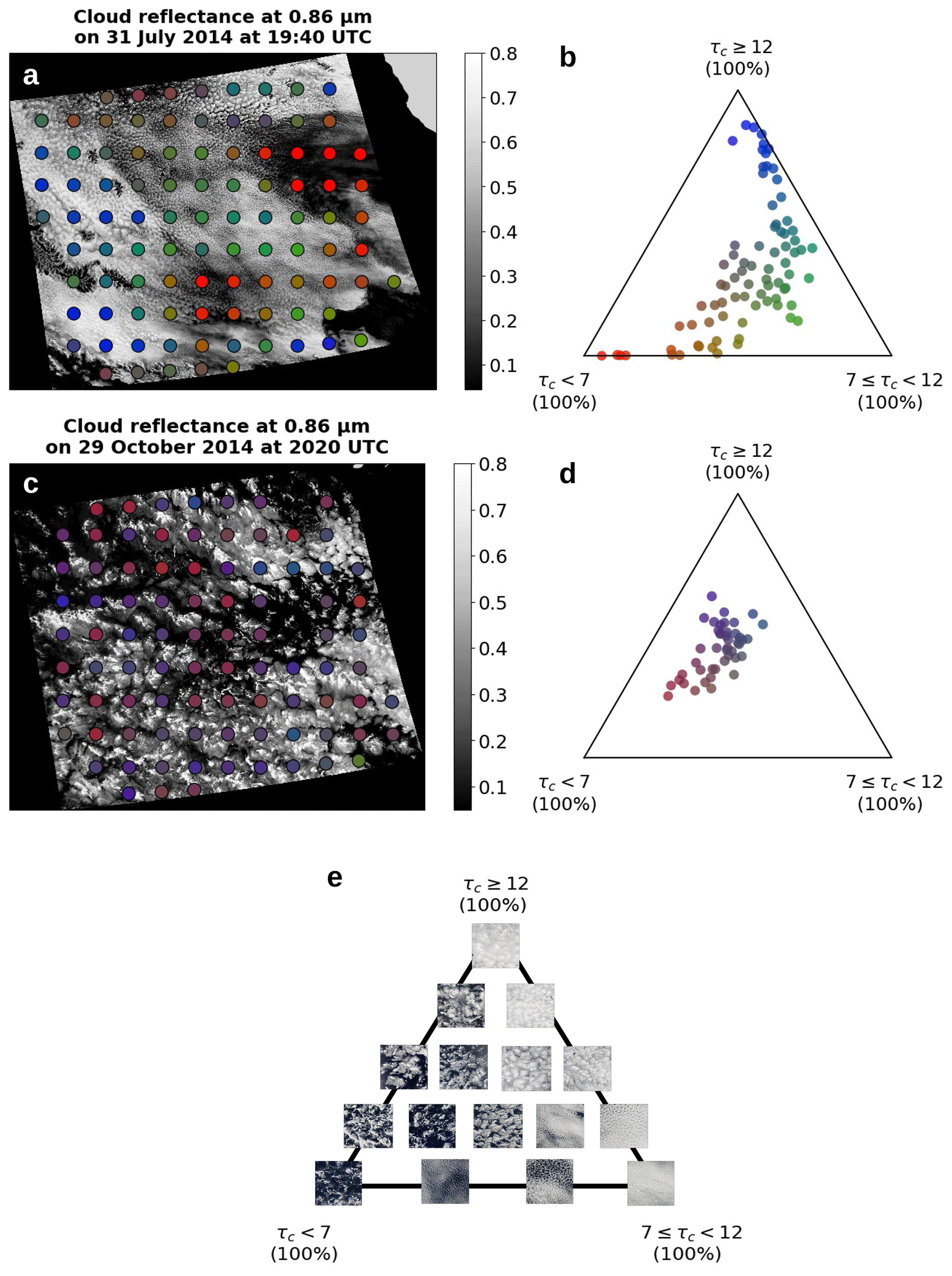
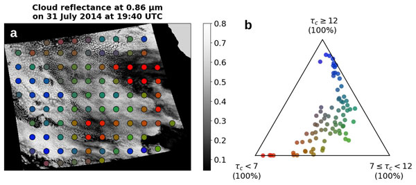
Figure 1 Examples of cloud morphology across the ternary morphology space. A ternary diagram illustrates the relative contributions of three components to a system, where each point represents the fractional contributions of the three components and each corner corresponds to 100 % of one component. The ternary corners are defined by τ_c classes: thin clouds (τ_c<7), intermediate clouds ($\mathrm{7}\le {\mathit{\tau }}_{\mathrm{c}}<\mathrm{12}$), and thick clouds (τ_c≥12). Panels (a) and (c) show MODIS reflectance at 0.86 µm, illustrating different cloud morphologies over the Pacific ocean East of North and South America, respectively. Each MODIS swath image is approximately 2330 km wide and 2100 km long. Panels (b) and (d) show the ternary diagram populated with 2°×2° scenes from the corresponding MODIS swaths in (a) and (c). Colored points represent the fractional contributions of the three τ_c classes as an RGB composite, with red corresponding to τ_c<7, green to $\mathrm{7}\le {\mathit{\tau }}_{\mathrm{c}}<\mathrm{12}$, and blue to τ_c≥12. Panel (e) shows MODIS true-color scenes illustrating common cloud morphologies across the ternary space. The scenes were selected such that their ternary composition matches their position within the ternary diagram.

The ternary space was discretized into evenly sized bins, each representing a unique τ_c morphology. 2°×2° scenes were assigned to a corresponding morphology bin within the ternary space, and microphysical statistical properties were computed for each bin. Bins containing fewer than 25 scenes were excluded from the analysis and are shown as NaN.

The τ_c class thresholds are defined on physical grounds, based on fundamental radiative transfer considerations: at τ_c≈7, A_c transitions from an approximately linear to a more logarithmic dependence on τ_c, and beyond τ_c≈12, any further increase in τ_c produces only minimal additional brightening of A_c. We also tested τ_c thresholds of 5 and 10 to align with the common definition of thin clouds as those having τ_c<5 (McCoy et al., 2023; Wood et al., 2018; Choudhury and Goren, 2024). The results did not change the key findings, and the main difference was a shift in the distribution of scenes within the ternary space.

2.2.2 Decomposing cloud susceptibilities

The ternary framework allows us to estimate cloud susceptibilities to N_d, conditioned on τ_c morphology. It should be emphasized that the ternary binning does not fix τ_c or other cloud properties within each morphology bin, as each bin retains natural variability in N_d, LWP, τ_c, A_c, and CF. This is evident, for example, in the difference between the LWP of cloud cores and that of the entire scene (Fig. 3c and d). Sensitivity tests in which the bin size was increased to allow greater variability in cloud properties within each bin did not affect the results. Transitions between morphology bins could have a stronger albedo response, such as in the case of transitions between closed and open cells (Goren and Rosenfeld, 2014; Watson-Parris et al., 2021), however these are temporally dependent (Goren et al., 2019) and not considered here.

A commonly used approach to estimate S_LWP from satellite observations is to regress dln LWP on dln N_d. However, when LWP and N_d are calculated under the adiabatic assumption using the satellite retrieved τ_c and r_e (Szczodrak et al., 2001), changes in r_e are expected to produce a linear sensitivity of −0.4 between dln LWP and dln N_d, assuming constant τ_c (Gryspeerdt et al., 2019). This effect was found to dominate S_LWP in our analysis (Fig. A2) because the variability in τ_c within each ternary bin is relatively small, as each bin is constrained by a τ_c class composition. To avoid this bias, S_LWP was calculated by subtracting the theoretical approximation of $S_{A_{\mathrm{c}}}$ (Platnick and Twomey, 1994; Twomey, 1991) from the satellite derived S_net. The residual is assumed to be primarily attributable to S_LWP, as shown below.

S_net (the in-cloud albedo susceptibility) can be written using the chain rule (Bellouin et al., 2020) as:

$$\begin{array}{}\text{(2)}& {\displaystyle }{\displaystyle }{S}_{\text{net}}\equiv {\displaystyle \frac{\mathrm{d}\ln A_{\mathrm{c}}}{\mathrm{d}\ln N_{\mathrm{d}}}}={\left.{\displaystyle \frac{\partial \ln A_{\mathrm{c}}}{\partial \ln N_{\mathrm{d}}}}\right|}_{\text{LWP}}+{\left.{\displaystyle \frac{\partial \ln A_{\mathrm{c}}}{\partial \ln \text{LWP}}}\right|}_{N_{\mathrm{d}}}{\displaystyle \frac{\mathrm{d}\ln \text{LWP}}{\mathrm{d}\ln N_{\mathrm{d}}}}.\end{array}$$

Here, S_net is defined as the susceptibility of in-cloud albedo to N_d, and therefore does not include adjustments in CF. This differs from formulations based on scene-mean albedo (Bellouin et al., 2020), where CF changes contribute an additional term. The first term on the right hand side represents the cloud albedo response to N_d, $S_{A_{\mathrm{c}}}$ (Twomey, 1991). Using the cloud albedo theoretical approximation (Twomey, 1991; Platnick and Twomey, 1994),

$$\begin{array}{}\text{(3)}& {\displaystyle }{\displaystyle }{S}_{A_{\mathrm{c}}}\equiv {\left.{\displaystyle \frac{\partial \ln A_{\mathrm{c}}}{\partial \ln N_{\mathrm{d}}}}\right|}_{\text{LWP}}={\displaystyle \frac{\mathrm{1}}{\mathrm{3}}}(\mathrm{1}-A_{\mathrm{c}}),\end{array}$$

where A_c is the in-cloud albedo of each 2°×2° scene. $S_{A_{\mathrm{c}}}$ is then averaged to obtain the mean $S_{A_{\mathrm{c}}}$ within each morphology bin, ${\stackrel{\mathrm{‾}}{S}}_{A_{\mathrm{c}}}$.

${\left.\frac{\partial \ln A_{\mathrm{c}}}{\partial \ln \text{LWP}}\right|}_{N_{\mathrm{d}}}$ in Eq. (2) represents how changes in LWP modify A_c. Because A_c depends primarily on τ_c, and ${\mathit{\tau }}_{\mathrm{c}}\propto {\text{LWP}}^{\mathrm{5}/\mathrm{6}}{N}_{\mathrm{d}}^{\mathrm{1}/\mathrm{3}}$ (Platnick and Twomey, 1994; Twomey, 1991), we can write:

$$\begin{array}{}\text{(4)}& {\displaystyle }{\displaystyle }\mathit{\gamma }\equiv {\left.{\displaystyle \frac{\partial \ln A_{\mathrm{c}}}{\partial \ln \text{LWP}}}\right|}_{N_{\mathrm{d}}}={\left.{\displaystyle \frac{\mathrm{5}}{\mathrm{6}}}{\displaystyle \frac{\partial \ln A_{\mathrm{c}}}{\partial \ln {\mathit{\tau }}_{\mathrm{c}}}}\right|}_{N_{\mathrm{d}}}={\displaystyle \frac{\mathrm{5}}{\mathrm{6}}}(\mathrm{1}-A_{\mathrm{c}})\end{array}$$

so that Eq. (2) becomes:

$$\begin{array}{}\text{(5)}& {\displaystyle }{\displaystyle }{S}_{\text{net}}\equiv {\displaystyle \frac{\mathrm{d}\ln A_{\mathrm{c}}}{\mathrm{d}\ln N_{\mathrm{d}}}}=S_{A_{\mathrm{c}}}+\mathit{\gamma }{\displaystyle \frac{\mathrm{d}\ln \text{LWP}}{\mathrm{d}\ln N_{\mathrm{d}}}}.\end{array}$$

For each morphology bin, we estimate S_net by regressing the observed ln A_c on ln N_d using all scenes within that bin. For consistency with $S_{A_{\mathrm{c}}}$, we use the bin mean in-cloud albedo, $\stackrel{\mathrm{‾}}{A_{\mathrm{c}}}$ in γ, so that $\stackrel{\mathrm{‾}}{\mathit{\gamma }}=\frac{\mathrm{5}}{\mathrm{6}}(\mathrm{1}-\stackrel{\mathrm{‾}}{A_{\mathrm{c}}})$. Evaluating Eq. (2) at each morphology bin gives:

$$\begin{array}{}\text{(6)}& {\displaystyle }{\displaystyle }{S}_{\text{net}}={\stackrel{\mathrm{‾}}{S}}_{A_{\mathrm{c}}}+\stackrel{\mathrm{‾}}{\mathit{\gamma }}{\displaystyle \frac{\mathrm{d}\ln \text{LWP}}{\mathrm{d}\ln N_{\mathrm{d}}}}.\end{array}$$

Solving for S_LWP yields S_LWP per morphology bin:

$$\begin{array}{}\text{(7)}& {\displaystyle }{\displaystyle }{S}_{\text{LWP}}\equiv {\displaystyle \frac{\mathrm{d}\ln \text{LWP}}{\mathrm{d}\ln N_{\mathrm{d}}}}={\displaystyle \frac{S_{\text{net}}-{\stackrel{\mathrm{‾}}{S}}_{A_{\mathrm{c}}}}{\stackrel{\mathrm{‾}}{\mathit{\gamma }}}}.\end{array}$$

S_LWP may implicitly include the influence of CF adjustments on the sampled in-cloud LWP, consistent with previous LWP adjustment studies (Gryspeerdt et al., 2019; Possner et al., 2020; Mülmenstädt et al., 2024).

S_CF, defined as the CF susceptibility to N_d, was calculated by regressing the observed ln (CF) on ln (N_d) for each ternary bin. Explicitly disentangling S_LWP from S_CF is challenging, as it is not uniquely defined how spatially heterogeneous changes in LWP should be attributed to variations in CF (Hoffmann et al., 2025).

3 Results

3.1 Examples of cloud morphology represented in ternary space

Figure 1a and c show two MODIS swaths containing different cloud morphologies. Figure 1b and d show the corresponding 2°×2° scenes from these swaths mapped onto the ternary diagram. Homogeneous scenes, in which the cellular structure is weakly expressed, are located near the corners of the ternary diagram, whereas inhomogeneous scenes with a more pronounced cellular structure are positioned away from the corners due to their mixed τ_c composition.

The cloud morphology can be seen to vary with CF, cell horizontal scale (large vs. small cells), and cloud reflectance, which can differ among cells of similar size. This means that cells with similar horizontal scales can be associated with different morphologies when their scene mean cloud albedo (or τ_c) is different. This extends the study of Zhou and Feingold (2023), which focused on classifying cell morphology by size, by additionally highlighting the role of τ_c variability across cells of similar size.

The morphologies in Fig. 1a are predominantly overcast, with homogeneous scenes appearing either as thin stratus layers (red points in Fig. 1a and b) or as thick closed cells (blue points in Fig. 1a and b). Between these lie heterogeneous morphologies with stronger contrast between cell cores and their surrounding clouds, reflecting a mixture of τ_c classes.

Figure 1c shows scenes of broken CF and closed cells with larger horizontal extent. These scenes typically correspond to precipitating clouds composed of thick cores (τ_c≥12 class) surrounded by a relatively large fraction of thin clouds (τ_c<7 class) (Wood et al., 2018; O et al., 2018), with only a limited contribution from the moderate τ_c class ($\mathrm{7}\le {\mathit{\tau }}_{\mathrm{c}}<\mathrm{12}$). This distinct morphology places these scenes farther toward the left side of the ternary diagram.

3.2 Occurrence of cloud morphologies

3.2.1 Observations

Figure 2a shows the 2015 distribution of scenes within the ternary morphology space. The most frequent morphologies are composed of a mixture of homogeneous optically thick and homogeneous optically thin clouds, with a relatively small contribution from the intermediate τ_c class. This implies that most of the variability in scene morphology arises from changes in the relative contributions of the thick and thin τ_c classes, whereas the fractional contribution of the intermediate τ_c class is relatively low. Such a mixtures of τ_c classes characterize active convective cores that coexist with thin clouds diverging from the cloud tops (Wood et al., 2018; Choudhury and Goren, 2024; O et al., 2018). The example in Fig. 1c and d shows this morphological type, consisting primarily of open cells and disorganized mesoscale cellular convection (Muhlbauer et al., 2014). Similar spatial variability in LWP has been used to distinguish disorganized mesoscale cellular convection from closed and open cells, and from stratus cloud layers with no cellular structure (Wood and Hartmann, 2006; Muhlbauer et al., 2014).

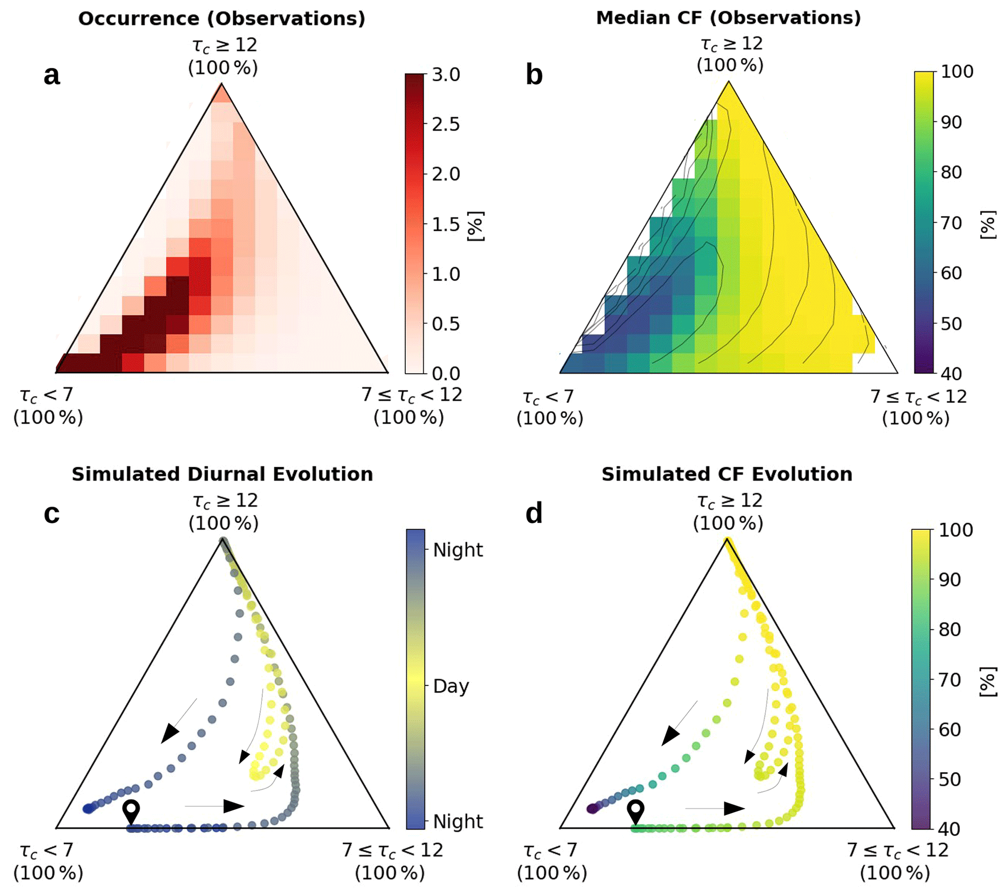
Figure 2 Ternary diagrams of scene occurrence and cloud fraction for satellite observations and LES. (a) Occurrence of 2°×2° scenes from one year (2015) of MODIS Aqua observations of marine low clouds having CF>40 %. Percentages represent the relative contribution of each morphology bin. (b) Median CF for each morphology bin, with contours indicating scene occurrence derived from (a). (c) LES simulation of overcast closed cells transitioning to open cells over a 24 h period, with time indicated by the color bar. (d) Same as (c), but showing CF. Arrows indicate the direction of the temporal evolution across the ternary space, with the pin icon indicating the beginning of the simulation. The closed-loop represents daytime cloud thinning, with the recovery later in the day overlapping the preceding nighttime trajectory. The simulated rate of change of the morphology can be inferred from the spacing between successive points.

The least frequent morphologies correspond to homogeneous scenes with intermediate τ_c. Interestingly, the scene-mean τ_c of all sampled scenes falls within this τ_c class, with an average value of approximately 9. This means that scene means often reflect a mixture of thick and thin clouds and are therefore not representative of the underlying τ_c distribution. Indeed, Goren et al. (2023) showed that relying on the scene-mean τ_c, rather than accounting for its spatial variability, can lead to a substantial bias in $S_{A_{\mathrm{c}}}$. Another less frequent morphology appears near the very left side of the ternary, where scenes are dominated by a mixture of thick and thin clouds, with minimal contribution from the intermediate τ_c class.

Figure 2b shows the median CF per ternary bin, revealing a clear separation between overcast and broken scenes. This indicates that overcast and broken scenes are associated with different τ_c morphologies. The highest scene occurrence (Fig. 2a) is found for broken cloud morphologies, consistent with previous studies. These scenes are attributed to the high occurrence of disorganized mesoscale cellular convection (Muhlbauer et al., 2014; Goren et al., 2025). The analysis therefore mainly represents stratocumulus clouds, primarily closed and open cells, disorganized mesoscale cellular convection, and stratus layers with no cellular pattern.

3.2.2 Large eddy simulations

Figure 2c and d show the morphology evolution of simulated clouds obtained from a Lagrangian LES of closed cells transitioning to open cells (Goren et al., 2019). The simulated clouds evolve along a morphology trajectory that closely matches the region of highest occurrence in the observations (Fig. 2a). This suggests that most observed scenes lie within the stratocumulus morphology evolution space that the analysis is designed to represent.

The simulated evolution of the cloud morphology also provides insight into key cloud processes. One example is cloud thickening during nighttime at the beginning of the simulation, driven by cloud top radiative cooling (Goren et al., 2019). Another is the diurnal cycle in cloud morphology, evident from the daytime loop feature in Fig. 2c and d. The loop feature shows an increased contribution from the intermediate τ_c class at the expense of the high τ_c class during the daytime morphology evolution (Fig. 2c), implying cloud thinning. It is driven by the daytime increase in solar radiation, which leads to cloud thinning and CF reduction (Fig. 2d) through warming and evaporation (Hignett, 1991; Meskhidze et al., 2009). Interestingly, the afternoon cloud thickening follows the same morphological trajectory as the cloud thickening during the previous night, suggesting a preferred evolutionary path. This can explain why the observed cloud morphologies do not span the entire ternary space but instead are concentrated along a preferred region within the morphology space (Fig. 2a). It remains an open question for future study whether a given morphological state can be reached through different paths.

The ternary representation also captures the rapid cloud breakup, indicated by the downward-pointing arrows in Fig. 2c and d. Because cloud breakup occurs concurrently with the development of substantial precipitation (Goren et al., 2019; Rosenfeld et al., 2006), scenes occupying this morphology space are presumably associated with collision and coalescence processes (Wang and Feingold, 2009).

The above demonstrates that the distribution of scenes within the ternary space encodes information about underlying cloud processes, such as cloud thickening, thinning, and collision–coalescence. Satellite observations projected onto the ternary space can therefore provide information about the state of the cloud field, as different regions of the diagram correspond to distinct cloud processes.

3.3 Cloud properties across the ternary morphology space

Figure 3 shows the microphysical properties across the ternary morphology space. In morphology bins characterized by low CF (Fig. 2b), N_d is relatively low and r_e exceeds 15 µm (Fig. 3a and b). This suggests that precipitation-driven breakup of overcast clouds could lead to the observed lower CF (Rosenfeld et al., 2006; Stevens et al., 2005; Wang and Feingold, 2009; Goren et al., 2019).

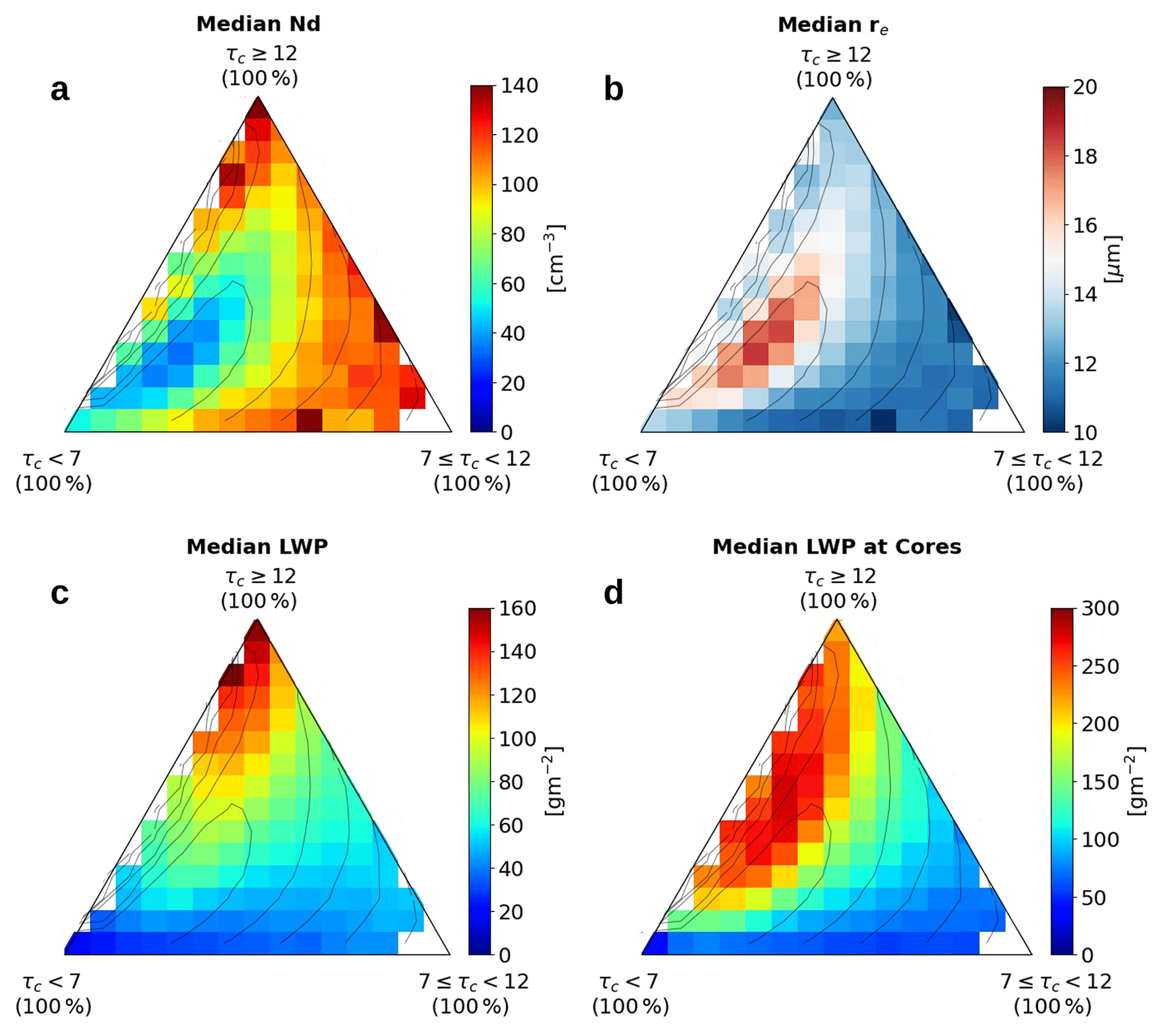
Figure 3 Median ternary-bin values of (a) N_d, (b) r_e, (c) LWP, and (d) cloud-core LWP, defined as the mean LWP of the 10 % of pixels with the highest LWP in each scene. Contours indicate scene occurrence, as in Fig. 2b.

An interesting pattern emerges in the LWP field (Fig. 3c). High LWP extends from the high τ_c class toward the low τ_c class (thin clouds), along the left side of the ternary. This pattern is somewhat counterintuitive because one might expect high LWP to extend toward the intermediate τ_c class. The reason becomes clear in Fig. 3d, which shows the LWP of the cloud cores, defined as the 10 % of pixels with the largest LWP. The core LWP is largest along the left side of the ternary, extending toward the lower τ_c class, indicating that the cores remain thick while an increasing fraction of surrounding pixels is gradually replaced by thinner clouds. This morphology is characteristic of stratocumulus in a deep boundary layer, where cloud-top divergence creates thin cloud layers at the top of the boundary layer (Wood et al., 2018; O et al., 2018; Goren et al., 2023; Choudhury and Goren, 2024). It reflects a morphological progression associated with the stratocumulus to cumulus transition (Bretherton and Wyant, 1997; Wyant et al., 1997), consistent with the examples in Fig. 1c and d, as well as with the simulated closed to open cloud trajectory (Fig. 2c and d).

At the left corner of the ternary diagram (the τ_c<7 class), scenes have low LWP. These scenes can be associated with the early stages of stratocumulus formation, typically appearing as an optically thin cloud layer lacking cellular structure (Fig. 1a, red points), or with the late stages of dissipating precipitating cells that leave remnants of thin cloud layers near the top of the boundary layer (Choudhury and Goren, 2024; Wood et al., 2018; O et al., 2018). The simulated morphology evolution further supports that clouds both form and dissipate near the lowest τ_c class (Fig. 3c and d).

3.4 Morphology-conditioned cloud susceptibilities

3.4.1 LWP susceptibility

Figure 4a shows that S_LWP is negative across the entire ternary space. This contrasts with previous studies that reported both positive and negative S_LWP, with the positive values attributed to precipitation suppression (Gryspeerdt et al., 2019; Possner et al., 2020). The negative S_LWP indicates that entrainment-related evaporation processes dominate across all morphologies, leading to a reduction in LWP as droplet size decreases with increasing N_d (Bretherton et al., 2007; Hoffmann et al., 2025; Pincus and Baker, 1994; Wood, 2007). The strongest S_LWP of nearly −1 is found in morphology bins where the intermediate τ_c class is dominant. In these scenes the horizontal cell sizes are relatively small (Fig. 4a), consistent with Zhou and Feingold (2023), who found similarly strong S_LWP in nonprecipitating small closed cells.

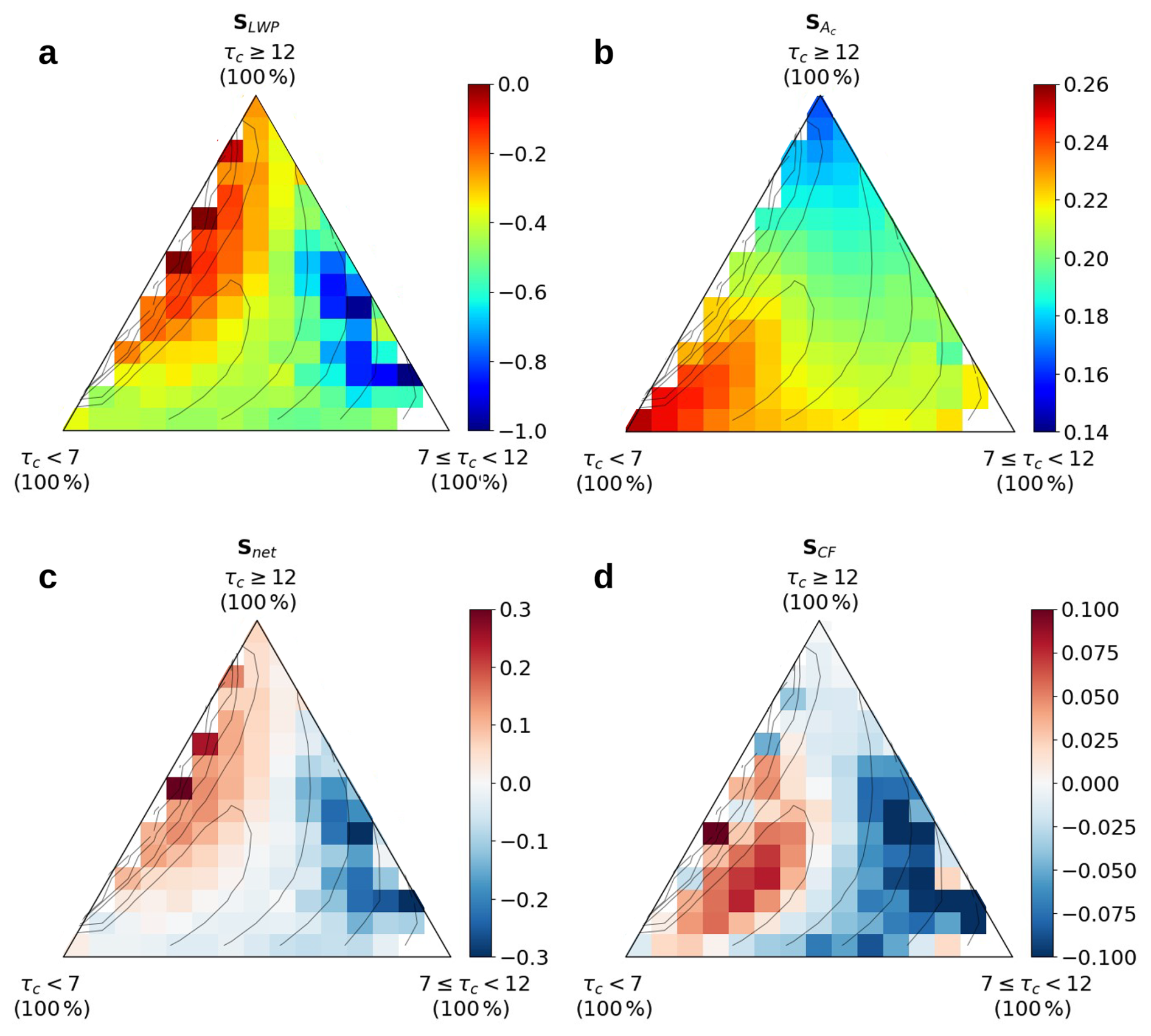
Figure 4 Susceptibilities to N_d of (a) LWP, (b) A_c (Twomey effect), (c) net cloud albedo, and (d) CF. Contours represent scene occurrence, as in Fig. 2b.

S_LWP weakens (becomes less negative) as the contribution from the intermediate τ_c class decreases and is replaced by increasing contributions from the lowest and highest τ_c classes. This partly coincides with an increase in r_e to values close to 15 µm (Fig. 3b), indicating the presence of precipitation (Rosenfeld et al., 2012), and suggests that precipitation suppression contributes to the weakened S_LWP, but not sufficiently to reverse its sign. Additionally, the dominance of thin cloud layers in these morphologies tends to be associated with more quiescent turbulent conditions (Wood et al., 2018), limiting their ability to entrain free-tropospheric air and thus constraining S_LWP. Our findings are consistent with Goren et al. (2025), who showed that the positive S_LWP reported for precipitating scenes in many inverted-V studies (Gryspeerdt et al., 2019; Mülmenstädt et al., 2024; Glassmeier et al., 2021; Possner et al., 2018) does not necessarily reflect precipitation suppression, but can instead arise as an artifact of aggregated sampling across different cloud morphologies.

The weakest S_LWP is found in morphologies composed of a mixture of thick and thin τ_c classes, with minimal contribution from the intermediate τ_c class. These morphologies are characterized by relatively large cell sizes (Fig. 1c) and r_e close to or exceeding 15 µm (Fig. 3), indicating mature closed cells approaching breakup (Goren et al., 2022; Choudhury and Goren, 2024). This is consistent with Zhou and Feingold (2023), who reported weak S_LWP for the largest cell sizes. In addition to delayed cloud breakup due to the delayed onset of precipitation, the weak S_LWP in these morphologies may also arise from differences in entrainment efficiency between thick cloud cores and the surrounding thin clouds (Zhou and Feingold, 2023; Bretherton et al., 2007; Kazil et al., 2017). Additionally, the non-negligible contribution of the highest τ_c class indicates the presence of thick, dynamically active cores, as evidenced by the large core-LWP (Fig. 1d). These cores likely supply cloud water to the diverging thinner clouds at their tops, which could partially offset LWP losses due to entrainment-driven evaporation, thereby further weakening the negative LWP response.

3.4.2 Cloud albedo susceptibility

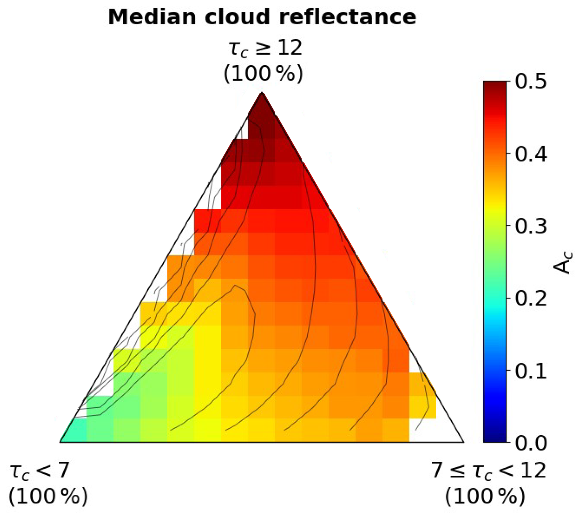
Figure 4b shows that the strongest $S_{A_{\mathrm{c}}}$ occurs in the lowest τ_c class and extends toward the top corner, towards the highest τ_c class, with the largest gradient along the left side of the ternary diagram. This is consistent with the theoretical approximation of $S_{A_{\mathrm{c}}}$ (Platnick and Twomey, 1994; Twomey, 1991), which predicts the largest susceptibility for scenes with the lowest A_c (see Fig. A3 for the distribution of A_c across the ternary space).

3.4.3 Net albedo susceptibility

Figure 4c shows a strong dependence of S_net on cloud morphology. S_net is negative in scenes dominated by intermediate τ_c classes and shifts toward positive values as the morphology becomes dominated by a mixture of thick and thin τ_c classes. The similarity between the morphological dependence of S_net and S_LWP (Fig. 4a) arises because $S_{A_{\mathrm{c}}}$ (Fig. 4b) exhibits relatively little variability compared to S_LWP. This indicates that S_net is primarily controlled by S_LWP. The strong influence of LWP adjustments on the net albedo response can also be shown theoretically (Feingold and Siebert, 2009).

The strongest negative S_net is found in scenes dominated by the intermediate τ_c class, where S_LWP outweighs the relatively strong in-cloud albedo response associated with the Twomey effect, $S_{A_{\mathrm{c}}}$ (Fig. 4b). This is consistent with Zhang et al. (2022), who found that thicker non-precipitating clouds, which likely correspond to the intermediate τ_c class here, exhibit cloud darkening. The strongest positive S_net, on the other hand, occurs where S_LWP is weakest, that is, least negative (Fig. 4a), allowing the Twomey brightening ($S_{A_{\mathrm{c}}}$) to enhance A_c without being substantially offset by the LWP adjustments.

Both the strongest negative and the strongest positive S_net are associated with the least frequent morphologies (Fig. 2a), whereas for the most frequent morphologies, S_LWP and $S_{A_{\mathrm{c}}}$ approximately balance each other, resulting in S_net near zero. As a result, the global mean S_net is relatively small, with a value of approximately $\mathrm{0.015}\pm \mathrm{0.007}.$ The uncertainty of the weighted mean slope was estimated from the variability across bin-specific slopes, accounting for the effective sample size. A substantial offset of the Twomey induced brightening by LWP adjustments has also been reported in previous studies (Prabhakaran et al., 2023; Toll et al., 2019; Diamond et al., 2020). It should be noted that the global mean S_net reflects the morphological occurrence of the year analyzed here. A future study will explore whether there are interannual differences in morphological occurrence, for example during El Nino years, as well as across seasons and regions.

3.4.4 Cloud cover susceptibility

The LWP and A_c susceptibility analysis focused on in-cloud changes, without considering changes in CF. Here, we further examine S_CF (Fig. 4d). Positive S_CF is found in precipitating scenes, as indicated by r_e>15 µm (Fig. 3b), consistent with studies reporting a positive relationship between CF and N_d (Rosenfeld et al., 2019; Chen et al., 2014; Wall et al., 2022; Goren and Rosenfeld, 2014). Since stratocumulus breakup is driven by the formation of precipitation (Goren et al., 2019, 2022; Yamaguchi et al., 2017), the positive S_CF reflects the effect of increased N_d in slowing precipitation formation, which slows down the reduction of CF.

Negative values of S_CF, by contrast, are found in non-precipitating scenes (r_e<15 µm). These scenes are composed primarily of the intermediate τ_c class, where S_LWP is strong and negative (Fig. 4a). This suggests that the negative strong S_LWP drives the negative S_CF. The scene-mean LWP in these morphology bins is relatively low (Fig. 3c), such that evaporation of cloud water associated with the strong S_LWP presumably leads to cloud dissipation and, consequently, a reduction in CF. We assume that the reduction in CF is associated with the thinner clouds at the edges of the cells (see examples in Fig. 1e), consistent with the assumptions in Goren and Rosenfeld (2014). The daytime cloud thinning and the associated small reduction in CF shown in Fig. 2c and d correspond to the negative S_CF shown in in Fig. 4d, consistent with the reported daytime decrease in CF (Hignett, 1991; Meskhidze et al., 2009). Weak negative S_CF are found where scenes are dominated by the thickest τ_c class. In these scenes, clouds are thick and have high LWP, so changes in LWP do not substantially affect scene CF.

4 Conclusions

We have introduced a new method for defining stratocumulus cloud morphologies using a ternary diagram. The ternary is composed of three τ_c classes and provides a continuous morphology space, in contrast to commonly used discrete cloud morphology regime classifications (Wood and Hartmann, 2006; Muhlbauer et al., 2014; Erfani and Hosseinpour, 2025; Wu et al., 2025; Yuan et al., 2020; Geiss et al., 2024). Using one year of satellite observations, we quantify the occurrence of scenes across the morphology space, revealing a preference for a confined range of morphologies. Complemented by LES, we show that cloud morphology evolution follows a preferred path across the ternary morphology space, explaining why most observations fall within a confined range of morphologies. The ternary framework also reveals insights into cloud processes associated with morphology changes, including cloud thickening, the diurnal cycle, and cloud breakup driven by precipitation. This suggests that the ternary encodes information about cloud processes that can be inferred from instantaneous satellite snapshots when projected into this space. The analysis also shows that scenes are often composed of mixtures of thick and thin clouds, making scene-mean values of spatially varying cloud properties, such as LWP and τ_c, not representative of the underlying cloud field. Using these means can therefore introduce biases in quantities that rely on these mean values (Goren et al., 2023).

The ternary framework allows us to estimate the susceptibilities of LWP, CF, and A_c to N_d, conditioned on cloud morphology. S_LWP is found to be negative across all morphologies, including in precipitating ones, in contrast to studies that have reported positive S_LWP and attributed it to precipitation suppression (Dipu et al., 2022; Glassmeier et al., 2021; Gryspeerdt et al., 2019; Mülmenstädt et al., 2024; Possner et al., 2020). Our results support Goren et al. (2025), who showed that the positive S_LWP inferred from inverted-V joint histograms of LWP and N_d arises as an artifact of aggregated sampling across different cloud morphologies. The strength of the negative S_LWP is found to depend on morphology, even for non-precipitating clouds, consistent with Zhou and Feingold (2023). Earlier studies, however, often reported a bulk approximation for S_LWP (Gryspeerdt et al., 2019; Glassmeier et al., 2021; Possner et al., 2020), thereby not capturing the morphology-dependent variability. Detecting a morphology-dependent S_LWP was possible by treating morphology as an observed variable, which also reduces confounding aerosol–meteorology co-variability that has been suggested to produce spurious negative values of S_LWP (Goren et al., 2025; Mülmenstädt et al., 2024).

S_CF is found to be positive in precipitating scenes, presumably because increased N_d delays precipitation and, consequently, cloud breakup (Goren et al., 2019; Wang and Feingold, 2009; Yamaguchi et al., 2017). On the other hand, in non-precipitating scenes with low LWP, S_CF is found to be negative, presumably because the strong negative S_LWP in these scenes reduces CF through entrainment-related evaporation processes. It should be noted that scenes with negative S_CF occur less frequently than those with positive S_CF, indicating that positive S_CF dominates the global signal.

The net in-cloud albedo susceptibility, S_net, is the most relevant for the radiation budget because it includes the combined contributions of $S_{A_{\mathrm{c}}}$ and S_LWP. S_net is found to vary between −0.3–0.3 depending on cloud morphology, largely modulated by the strong control of S_LWP. This implies that, in some morphological regimes, Twomey-induced brightening is offset by LWP adjustments, consistent with findings from previous studies (Prabhakaran et al., 2023; Toll et al., 2019; Diamond et al., 2020). Here, we further show that this offset can fully cancel, and even exceed, the Twomey-induced brightening, leading to a net negative effect. When averaged over all morphologies, S_net is overall small (0.015±0.007), as it is dominated by the most frequently occurring morphologies, which have lower S_net. This implies that a global 10 % increase in N_d would result in an increase in cloud albedo of approximately 0.15±0.07 %, not accounting for changes in CF. The analysis suggests that marine cloud brightening would need to target morphologies with positive S_net and rely on persistently positive S_CF to be effective. The results also have implications for estimates of aerosol–cloud radiative forcing, which should account for morphology-weighted contributions.

Appendix A: Additional figures

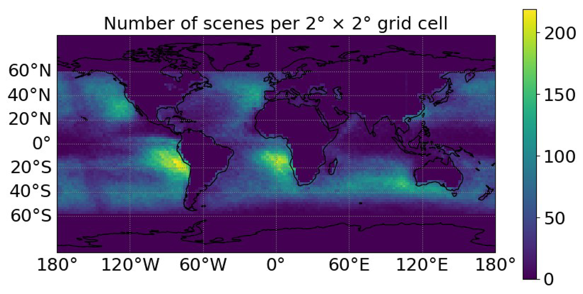
Figure A1 Number of scenes per 2°×2° grid cell used in the analysis. It can be seen that most scenes derive from the stratocumulus regions in the eastern subtropical oceans.

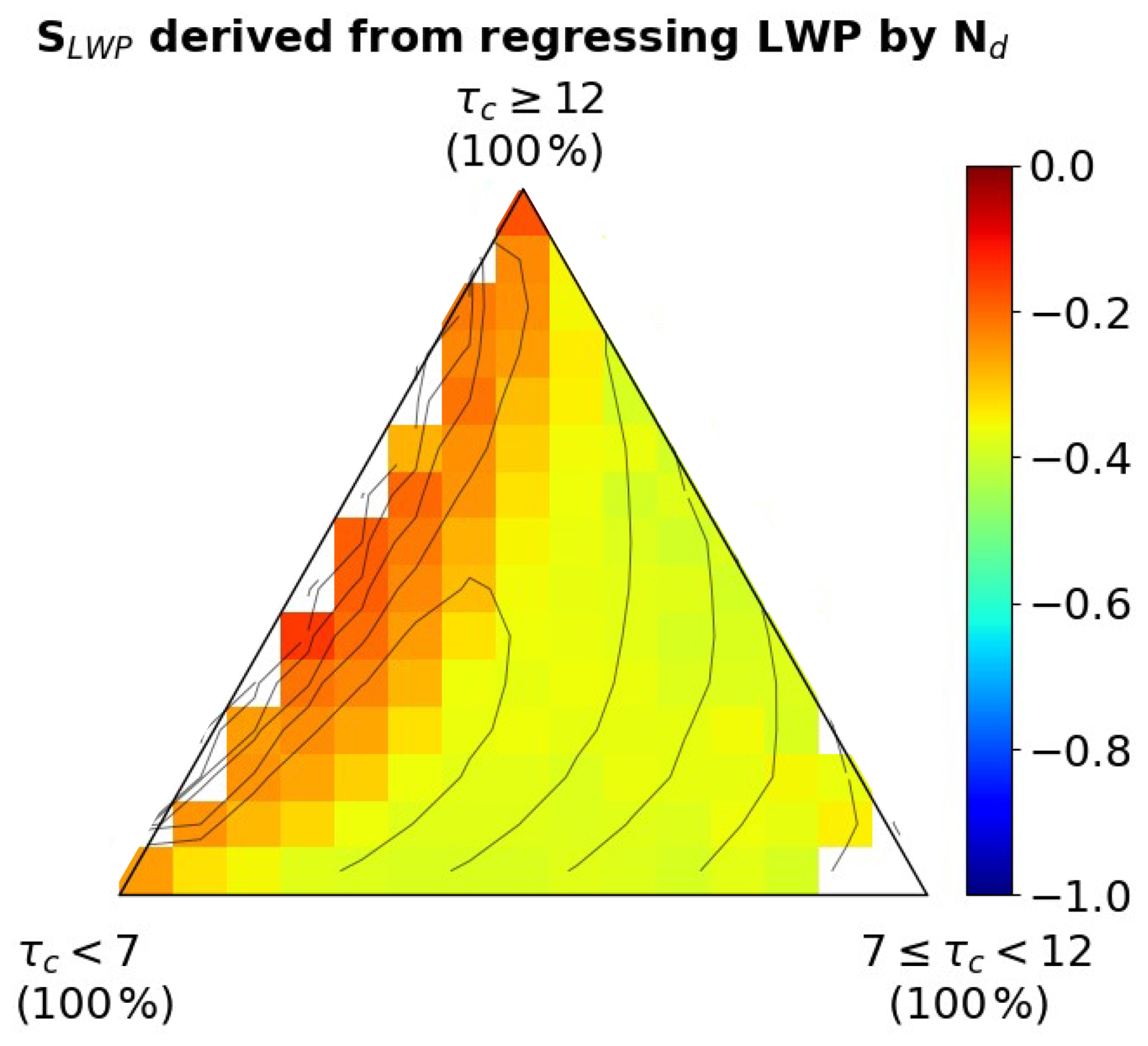
Figure A2 LWP susceptibility derived from the regression between ln LWP and ln N_d within each ternary bin. Contours represent scene occurrence, as in Fig. 2b.

Figure A3 Median ternary-bin values of A_c. Contours indicate scene occurrence, as in Fig. 2b.