Volcanic aerosol modification of the stratospheric circulation in E3SMv2 – Part 2: Brewer–Dobson Circulation

Great attention has been paid to the short-term climate response following explosive volcanic eruptions, in order to understand effects on zonal winds, the polar vortex, and surface temperature across latitude. In contrast, several works have shown that evidence of volcanic forcing can persist for much longer in the stratosphere's chemical composition, even after the instigating aerosol population has dissipated. Heating by volcanic aerosols accelerates tropical upwelling, and thus drives an acceleration of the Brewer–Dobson Circulation (BDC), and enhances troposphere–stratosphere mass exchange. Even after tropical motion returns to its climatological mean, the anomalous mass exchange remains detectable in the stratosphere for several years. In this work, we use an age-of-air (AoA) tracer to diagnose stratospheric composition changes following the simulated 1991 Mt. Pinatubo eruption. Specifically, we employ simulation ensembles from the E3SMv2 climate model to identify statistically significant effects on zonal-mean AoA. In addition, we use the Residual Circulation Transit Time (RCTT) diagnostic to separate the effects of advective transport and mixing. We find that the Mt. Pinatubo eruption lowers AoA in the middle-to-upper stratosphere globally, primarily due to an accelerated residual meridional circulation. We also observe a localized increase of AoA near 20–100 hPa in the southern hemisphere (the hemisphere opposite the eruption), which we attribute to a damping of the seasonal BDC cycle by the volcanic aerosols. We suggest that a dampened seasonal BDC cycle is perhaps a generic result of any heating process driven by aerosols that evolve on timescales beyond seasonal in the meridional plane.

1 Introduction

Large volcanic eruptions are capable of injecting very large quantities of sulfate aerosols into the stratosphere. In the years following such an eruption, temperature forcing by stratospheric volcanic aerosol concentrations plays an important role in the interannual variability of the climate, and leads to significant and persistent anomalous climate states. In the first part of this series of papers (Hollowed et al. (2025a); hereafter Part 1), we investigated the large-scale mechanisms that control post-eruption zonal wind anomalies using the Transformed Eulerian Mean (TEM) analysis framework. We saw that the wind response was intermittent, with a notable seasonal dependence, but that the timescale of both the temperature and wind anomalies is ultimately governed by the volcanic aerosol decay. From a climatological point of view, the response is approximately instantaneous with respect to the radiative forcing, and we generally expect that the stratospheric dynamics and aerosol concentrations will return to their climatological averages in tandem. In the simulations used in Part 1, this timescale is about two years.

We now turn our attention to the stratospheric composition. In Part 1, the meridional and vertical residual circulation (${\stackrel{\mathrm{‾}}{v}}^{*}$, ${\stackrel{\mathrm{‾}}{w}}^{*}$) was discussed, primarily with respect to its seasonal forcing of the zonal wind. This forcing mechanism, as expressed in the TEM framework, is a combination of direct advection of momentum and a Coriolis torque induced by the meridional component of the circulation. The strength of these effects develops and deteriorates over the year, with minimum (maximum) forcing in the summer (winter) hemisphere. This may naively lead us to conclude that the most important modes of stratospheric variability are essentially seasonal-to-annual. However, advection of trace gases by the residual circulation, and thus the genesis and depletion of stratospheric chemical concentrations, operates on much longer timescales. In this paper, it is shown that the volcanic effects on zonal temperature and momentum are progenitors of robust, decadal-scale anomalies in the distributions of trace gases in the stratosphere. It will be demonstrated that these anomalies are due to a global acceleration of the meridional Brewer–Dobson Circulation (BDC), but also a damping of the seasonal BDC cycle.

The BDC was first inferred and described in the works of Brewer (1949) and Dobson (1956) in an effort to explain observed concentrations of ozone, water vapor, and other stratospheric tracer constituents. This circulation approximates the mean Lagrangian transport of mass in the meridional plane as a superposition of the Eulerian mean circulation and an eddy-driven component accounting for the Stokes drift induced by the wave field (Dunkerton, 1978). Tracer isopleths (surfaces of constant mixing ratio) are raised and lowered in the tropics and polar regions, respectively, by the thermally-direct overturning cell that is the mean residual circulation. Throughout the stratosphere, breaking planetary waves cause vertical diabatic mixing across isentropes, and especially in the midlatitude surf-zone, isopleths are homogenized by two-way adiabatic mixing of mass along isentropes (e.g. Plumb, 2007). In other words, the BDC is essentially an expression of the TEM balance from a tracer perspective.

Through both observations and model studies, it is now understood that the full traversal of the BDC, in a Lagrangian sense, takes up to 5–7 years (Butchart, 2014; Waugh and Hall, 2002). This traversal timescale can be measured by the so-called stratospheric age of air (AoA), which has a rich history in the literature since at least the 1990s (see Waugh and Hall (2002) and Garny et al. (2024) for comprehensive reviews). The “age” of an air parcel is defined as the elapsed time since its last contact with some reference location, which is usually taken to be the tropical tropopause. In a modeling context, AoA is often implemented as a scalar “clock tracer” with a globally uniform and constant source, and gridpoint-level mixing ratios which correspond to the mean stratospheric age-of-air.

Early implementations were published by Hall and Prather (1993), Hall and Plumb (1994) and Neu and Plumb (1999). More recently, Gupta et al. (2020, 2021) implemented AoA tracers in a variety of dynamical cores to test their sensitivity to numerical schemes and spatial discretizations. Meanwhile, several recent works have made strides in disentangling the advective and eddy-driven components of the BDC, and their contributions to the climatological AoA distribution. A key development was by Birner and Bönisch (2011), who introduced the residual circulation transit time (RCTT), which identifies the age distribution arising purely from advective transport. The RCTT is obtained by solving for “backward trajectories” connecting each point in the latitude-altitude plane to a crossing of the tropopause, by integrating over the time-varying meridional and vertical residual circulation (${\stackrel{\mathrm{‾}}{v}}^{*}$, ${\stackrel{\mathrm{‾}}{w}}^{*}$) in reversed time. Later, Garny et al. (2014) pointed out that the difference (AoA − RCTT) could be used to approximately isolate aging by isentropic mixing, which throughout much of the upper atmosphere was shown to be at least as important as aging by residual circulation advection. While this type of differencing is a useful procedure, it is also a blunt one, as it cannot separate contributions of mixing by resolved wave breaking and diffusion. Nor can it identify any contributions by unresolved advective affects, such as recirculation of Lagrangian tracers, or nonlinear or transient wave contributions which affect the Lagrangian mean circulation, but are only partially represented in the residual circulation of the TEM.

On the other hand, we know from the analysis outlined in Part 1 that a more fine-grained decomposition of AoA tendencies should be theoretically feasible. Ploeger et al. (2015a, b) and Dietmüller et al. (2017) demonstrated a method to this end, by computing a set of RCTT trajectories, and then integrating the components of the eddy-tracer flux vector M in time over those trajectories.

AoA anomalies arising in response to both persistent and transient forcing sources are numerous in the literature. Long-term AoA trends in coupled historical simulations have been used to study the response of the BDC to anthropogenic climate change, where the typical finding is decreased age (an accelerated BDC) throughout the lower stratosphere (Muthers et al., 2016; Garfinkel et al., 2017; Ploeger et al., 2019; Abalos et al., 2021). In the case of the stratospheric aerosol injection (SAI) geoengineering simulation studies of Richter et al. (2017), the authors showed anomalies in the residual vertical velocity ${\stackrel{\mathrm{‾}}{w}}^{*}$ consistent with an accelerated BDC, but did not show the associated AoA effects. Several works have also concluded a likely accelerated BDC after large volcanic eruptions (Pitari, 1993; Eluszkiewicz et al., 1996; Toohey et al., 2014), while some (Garcia et al., 2011; Pitari et al., 2016) have directly shown decreases in stratospheric AoA by several months for the 1991 Mt. Pinatubo event specifically.

The goal of the present article is to study the significant post-volcanic impacts on the AoA tendency balance, as we did for the zonal-mean zonal wind $\stackrel{\mathrm{‾}}{u}$ in Part 1. The key question is: what are the relative contributions of perturbed residual circulation advection and perturbed mixing in producing the net impact on stratospheric AoA post-eruption?

To this end, we draw some inspiration from adjacent works that pose the same problem to different tracer species. For example, Abalos et al. (2013) showed the closed TEM tracer budget in the meridional plane for ozone (O₃) and carbon monoxide (CO) over a 6-year dataset. In a generalization of this work, they later investigated the closed TEM budget for an artificial tracer called e90 (Abalos et al., 2017), which is defined such that its distribution is uniquely sensitive to perturbations to troposphere-stratosphere mass exchange. Therefore, e90 qualitatively resembles the behavior of real-world substances in this region, like ozone (O₃) and carbon monoxide (CO). The artificial e90 tracer is indeed a suitable proxy to investigate the impact of the Mt. Pinatubo volcanic eruption on the flow field as also outlined in Hollowed (2025). For conciseness, this aspect has not been included here, and we point the reader to the above reference.

In this work, we seek not to emulate the behavior of a real-world substance, but rather use the AoA tracer to understand the behavior of the stratospheric circulation itself. Section 2 describes the simulated datasets employed. Section 3 introduces the analysis framework, including the tracer definition, the tracer TEM balance, and the method of computing the RCTT. Section 4 presents the climatological behavior of AoA in our simulations, and Sect. 5 explores the identified impacts. Section 6 considers the sensitivity of the identified impacts with eruption magnitude, and Sect. 7 closes the paper with a discussion of the results and concluding remarks.

2 Simulations

The research is built upon the same simulations as in Part 1, described in detail in Sect. 2 therein. Briefly, we use the fully-coupled E3SMv2-SPA model (Brown et al., 2024) to simulate the eruption of Mt. Pinatubo as an emission of sulfur dioxide (SO₂) over 6 h and 9 grid cells between 18 and 20 km near 15° N, and evolve the resulting sulfate aerosols via a prognostic treatment. The simulations utilize a ∼ 1° horizontal grid and 72 vertical levels that extend to approximately 60 km, and feature an internally-generated QBO with a period of approximately 24 months (see Sect. 4.2 of Part 1). We again use the paired limited-variability volcanic ensemble (LV) and its counterfactual ensemble (CF), introduced by Ehrmann et al. (2024), for the impact analysis. Both ensembles include 15 members covering an approximately 7.5-year time period from 1 June 1991 to 1 January 1999. The CF ensemble omits the Mt. Pinatubo volcanic eruption, and each LV–CF member pair shares identical initial conditions. Statistically significant departures of the LV ensemble mean from the CF ensemble mean are therefore interpreted as the isolated volcanic impact. We primarily use the same 10 Tg SO₂ eruption as Part 1, while Sect. 6 additionally includes a brief analysis of the tracer sensitivity with respect to eruption magnitude. This is accomplished through additional LV ensembles with 3, 5, 7, 13, and 15 Tg SO₂ eruptions. All data products from the LV and CF ensembles were provided as daily-averaged fields.

The AoA is computed as a tracer mixing ratio at each gridpoint during the model run. Here, we will use the zonal mean of the daily-averaged tracer field. For computing the residual circulation transit time, the history of the daily-averaged residual velocity components ${\stackrel{\mathrm{‾}}{v}}^{*}$ and ${\stackrel{\mathrm{‾}}{w}}^{*}$ is required for a period of ten years prior to the time of analysis. A 10-year prior history was chosen so that the RCTT distribution would be well-represented in the time-averaged ensemble mean. This period needs to be long enough to represent transit times in regions with the longest backward trajectories, which tend to be the polar lower stratosphere. The choice of ten years was inspired by testing the RCTT calculation on our data and using guidance from previous studies. For example, Birner and Bönisch (2011) found that the longest transit times measured in their simulations were “4–5 years in the lowest stratosphere above the poles”. In addition, Garny et al. (2014) state that “10 years of data are sufficient to represent the mean state of the simulations”, while their climatological RCTT distributions also reach only 4–5 years in the polar lower stratosphere. We similarly found that our 5-year averaged ensemble mean RCTT distributions reached maxima of 5–6 years near the poles, but that individual backward trajectories in individual ensemble members may require up to ten years or more to cross the tropical tropopause. Choosing ten years does result in missing data for a few gridpoints in the polar lower stratosphere for some ensemble members (i.e. ten years was not long enough). Still, the missing data are minimal, and ten years was enough to converge on a well-represented, time-averaged, ensemble-mean RCTT distribution.

Because the LV ensembles were all initialized on 1 June 1991, we were required to concatenate the ${\stackrel{\mathrm{‾}}{v}}^{*}$ and ${\stackrel{\mathrm{‾}}{w}}^{*}$ time series from the LV runs, and the control simulation from which the perturbed LV ensemble initial conditions were seeded, in order to obtain a 10-year history. The concatenation of the control simulation and a single LV ensemble member is illustrated in Fig. 1 for a midlatitude gridpoint at 10 hPa. RCTT integration bounds for selected dates are plotted as a reference.

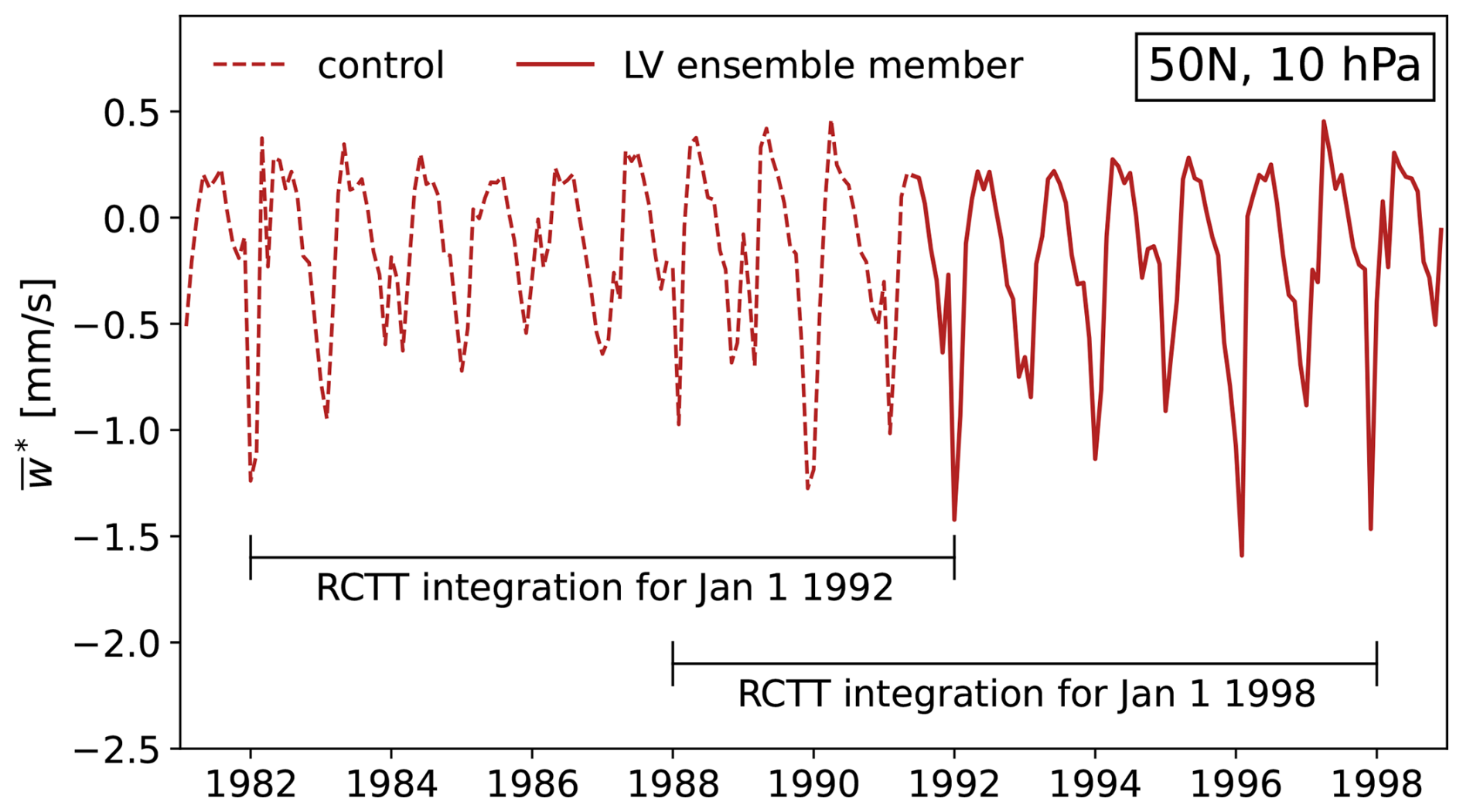
Figure 1 Concatenated time series of the residual vertical velocity ${\stackrel{\mathrm{‾}}{w}}^{*}$ at 50° N, 10 hPa for a single LV ensemble member (1 June 1991 to 1 January 1999; solid dark red line), and the control simulation (1 January 1982 to 1 June 1991; dark red dashed line). Two example RCTT integrations are annotated as bracketed black lines. The RCTT on 1 January 1992 is computed by residual velocity integration over the decade 1982–1992, and likewise for the RCTT on 1 January 1998 and the decade 1988–1998.

The control simulation was generated from E3SMv2-SPA with an equivalent configuration to the LV and CF runs, though in principle there are discontinuities at the concatenation point. In part, this is because the LV ensemble initialization involved random temperature perturbations on the order of 10⁻¹⁴ K to drive differences between the members. There is also a second instance of a temperature perturbation of the same magnitude on 1 January 1988 in the control simulation that was inherited from the parent dataset, and is unrelated to the present study. In addition, while the winds across the LV initialization point are approximately continuous, non-volcanic climate forcing sources are not. This is because the control and LV calendars are different, and needed to be manually aligned (again, this is due to an inherited experimental design that is unrelated to the present study; see Ehrmann et al. (2024) for full details). Because the RCTT results from long-time integrations over monthly-averaged ${\stackrel{\mathrm{‾}}{v}}^{*}$ and ${\stackrel{\mathrm{‾}}{w}}^{*}$, we expect the consequences of these features on the results to be negligible. To whatever extent that these discontinuities are present in the recovered transit times, they are present equally in the LV and CF ensembles, and thus will be removed when taking the (LV − CF) impact.

3 Analysis Framework

As in Part 1, we express the post-eruption anomalies in a variable x as impacts, defined as the ensemble mean of the difference between each pair of LV and CF simulations:

$$\begin{array}{}\text{(1)}& \mathrm{\Delta }x\equiv {\displaystyle \frac{\mathrm{1}}{N}}\sum _{n=\mathrm{1}}^N\left(x^{\left(n\right)}-x^{\mathrm{CF},\left(n\right)}\right).\end{array}$$

where N is the ensemble size, n is each ensemble member enumerated, x is the data from the volcanic simulation, and x^CF is the data from the counterfactual simulation. For assessing the statistical significance of the impact Δx, we use a two-sided Student's t-test with a p-value threshold of 0.05 (95 % confidence). See Sect. 3.1 of Part 1 for full details on the statistical calculations. Both a tracer form of the TEM equations and the RCTT will be used to diagnose the impacts on residual circulation advection and mixing separately. The tracer sources and sinks, as well as the TEM and RCTT formulations, are defined below.

3.1 Tracer definition

Tracers in E3SM are stored as dimensionless mixing ratios, i.e. (kg of tracer)$/$(kg of air), within each cell in the simulation grid. While this is an appropriate choice for material substances, the interpretation changes for the age of air tracer, which has an implicit unit of time. As such, we implemented the AoA tracer with a constant production rate of

$$\begin{array}{}\text{(2)}& {\displaystyle \frac{\partial \mathrm{AoA}}{\partial t}}={\displaystyle \frac{\mathrm{1}}{\mathrm{86}\mathrm{400}}}{\mathrm{s}}^{-\mathrm{1}}=\mathrm{1}{\mathrm{d}}^{-\mathrm{1}}.\end{array}$$

everywhere above 700 hPa. Below 700 hPa, we impose an “instantaneous sink”, by directly setting

$$\begin{array}{}\text{(3)}& \begin{array}{rl}& \mathrm{AoA}=\mathrm{0},\\ & {\displaystyle \frac{\partial \mathrm{AoA}}{\partial t}}=\mathrm{0}{\mathrm{s}}^{-\mathrm{1}}\end{array}\end{array}$$

The result is a tracer with a dimensionless mixing ratio that is equal in value to the mean age since last contact with the < 700 hPa layer, in number of days. This is similar to the implementation of Gupta et al. (2020), but with the source located above rather than below the lower-level threshold. The approach of Gupta et al. (2020) instead requires the subtraction of the model time from the AoA mixing ratios, but is functionally identical.

3.2 Tracer TEM framework

The TEM formulation for the time (t) evolution of a zonal-mean tracer mixing ratio $\stackrel{\mathrm{‾}}{q}$ is analogous to the formulation for zonal momentum $\stackrel{\mathrm{‾}}{u}$ (see Sect. 3.2 in Part 1) specified in spherical coordinates for the hydrostatic primitive equations on constant pressure levels by Gerber and Manzini (2016). The time tendency of $\stackrel{\mathrm{‾}}{q}$ is written as

$$\begin{array}{}\text{(4)}& {\displaystyle \frac{\partial \stackrel{\mathrm{‾}}{q}}{\partial t}}={\displaystyle \frac{\partial \stackrel{\mathrm{‾}}{q}}{\partial t}}{|}_{\left({\stackrel{\mathrm{‾}}{v}}^{*}\right)}+{\displaystyle \frac{\partial \stackrel{\mathrm{‾}}{q}}{\partial t}}{|}_{\left({\stackrel{\mathrm{‾}}{\mathit{\omega }}}^{*}\right)}+{\displaystyle \frac{\partial \stackrel{\mathrm{‾}}{q}}{\partial t}}{|}_{\mathrm{\nabla }\cdot \mathit{M}}+\stackrel{\mathrm{‾}}{X}+\stackrel{\mathrm{‾}}{S}.\end{array}$$

The first and second terms represent tracer advection by the residual circulation,

$$\begin{array}{}\text{(5)}& {\displaystyle \frac{\partial \stackrel{\mathrm{‾}}{q}}{\partial t}}{|}_{\left({\stackrel{\mathrm{‾}}{v}}^{*}\right)}=-{\stackrel{\mathrm{‾}}{v}}^{*}{\displaystyle \frac{\partial \stackrel{\mathrm{‾}}{q}\cos \mathit{\varphi }}{\cos \mathit{\varphi }\partial \mathit{\varphi }}}\text{(6)}& {\displaystyle \frac{\partial \stackrel{\mathrm{‾}}{q}}{\partial t}}{|}_{\left({\stackrel{\mathrm{‾}}{\mathit{\omega }}}^{*}\right)}={\stackrel{\mathrm{‾}}{w}}^{*}{\displaystyle \frac{p}{H}}{\displaystyle \frac{\partial \stackrel{\mathrm{‾}}{q}}{\partial p}}\end{array}$$

The symbol ϕ denotes the latitude, and p stands for the pressure. The meridional and vertical residual velocities ${\stackrel{\mathrm{‾}}{v}}^{*}$ and ${\stackrel{\mathrm{‾}}{w}}^{*}$ are

$$\begin{array}{}\text{(7)}& {\displaystyle }{\stackrel{\mathrm{‾}}{v}}^{*}=\stackrel{\mathrm{‾}}{v}-{\displaystyle \frac{\partial \mathit{\psi }}{\partial p}}\text{(8)}& {\displaystyle }{\stackrel{\mathrm{‾}}{w}}^{*}=-{\displaystyle \frac{H}{p}}{\stackrel{\mathrm{‾}}{\mathit{\omega }}}^{*}=-{\displaystyle \frac{H}{p}}\left(\stackrel{\mathrm{‾}}{\mathit{\omega }}+{\displaystyle \frac{\partial \mathit{\psi }\cos \mathit{\varphi }}{a\cos \mathit{\varphi }\partial \mathit{\varphi }}}\right)\end{array}$$

where ω is the vertical pressure velocity, v is the meridional velocity, and the eddy streamfunction ψ is

$$\begin{array}{}\text{(9)}& \mathit{\psi }={\displaystyle \frac{\stackrel{\mathrm{‾}}{v^{\prime }{\mathit{\theta }}^{\prime }}}{\partial \stackrel{\mathrm{‾}}{\mathit{\theta }}/\partial p}}\end{array}$$

where θ is the potential temperature. The residual streamfunction Ψ^* is defined as

$$\begin{array}{}\text{(10)}& {\mathrm{\Psi }}^{*}={\displaystyle \frac{\mathrm{2}\mathit{\pi }a\cos \mathit{\varphi }}{g_{\mathrm{0}}}}\left(\underset{p}{\overset{\mathrm{0}}{\int }}{\stackrel{\mathrm{‾}}{v}}^{*}\mathrm{d}p\right),\end{array}$$

with g₀ as the global-mean gravitational acceleration at mean sea level. The third term on the right of Eq. (4) is the eddy-driven tracer mixing tendency,

$$\begin{array}{}\text{(11)}& {\displaystyle \frac{\partial \stackrel{\mathrm{‾}}{q}}{\partial t}}{|}_{\mathrm{\nabla }\cdot \mathit{M}}={\displaystyle \frac{\mathrm{\nabla }\cdot \mathit{M}}{a\cos \mathit{\varphi }}}.\end{array}$$

The vector M is the eddy-tracer flux vector, with meridional and vertical components

$$\begin{array}{}\text{(12)}& {\displaystyle }{M}_{\left(\mathit{\varphi }\right)}=a\cos \mathit{\varphi }\left({\displaystyle \frac{\partial \stackrel{\mathrm{‾}}{q}}{\partial p}}\mathit{\psi }-\stackrel{\mathrm{‾}}{q^{\prime }{v}^{\prime }}\right)\text{(13)}& {\displaystyle }{M}_{\left(p\right)}=a\cos \mathit{\varphi }\left(-{\displaystyle \frac{\partial \stackrel{\mathrm{‾}}{q}\cos \mathit{\varphi }}{a\cos \mathit{\varphi }\partial \mathit{\varphi }}}\mathit{\psi }-\stackrel{\mathrm{‾}}{q^{\prime }{\mathit{\omega }}^{\prime }}\right),\end{array}$$

and the eddy-tracer flux divergence (ETFD) is

$$\begin{array}{}\text{(14)}& \mathrm{\nabla }\cdot \mathit{M}={\displaystyle \frac{\partial M_{\left(\mathit{\varphi }\right)}\cos \mathit{\varphi }}{a\cos \mathit{\varphi }\partial \mathit{\varphi }}}+{\displaystyle \frac{\partial M_{\left(p\right)}}{\partial p}}\end{array}$$

where a denotes the Earth's radius. These forms are analogous to the Eliassen–Palm (EP) flux vector and its divergence which governs the TEM momentum forcing by resolved waves, used in Part 1.

The final terms of Eq. (4), $\stackrel{\mathrm{‾}}{X}$ and $\stackrel{\mathrm{‾}}{S}$, are the forcing by parameterized processes and diffusion, and the net tracer sources and sinks, respectively. As we did for the TEM momentum equation in Part 1, $\stackrel{\mathrm{‾}}{X}$ is inferred by taking the difference between the sum of Eqs. (5)–(11) and the net tendency $\partial \stackrel{\mathrm{‾}}{q}/\partial t$:

$$\begin{array}{}\text{(15)}& \stackrel{\mathrm{‾}}{X}={\displaystyle \frac{\partial \stackrel{\mathrm{‾}}{q}}{\partial t}}-{\displaystyle \frac{\partial \stackrel{\mathrm{‾}}{q}}{\partial t}}{|}_{\left({\stackrel{\mathrm{‾}}{v}}^{*}\right)}-{\displaystyle \frac{\partial \stackrel{\mathrm{‾}}{q}}{\partial t}}{|}_{\left({\stackrel{\mathrm{‾}}{\mathit{\omega }}}^{*}\right)}-{\displaystyle \frac{\partial \stackrel{\mathrm{‾}}{q}}{\partial t}}{|}_{\mathrm{\nabla }\cdot \mathit{M}}-\stackrel{\mathrm{‾}}{S}.\end{array}$$

The net tendency, which was not available as a model output, is estimated by a first-order finite difference taken on the daily-mean $\stackrel{\mathrm{‾}}{q}$ data, as

$$\begin{array}{}\text{(16)}& {\displaystyle \frac{\partial \stackrel{\mathrm{‾}}{q_i}}{\partial t}}={\displaystyle \frac{{\stackrel{\mathrm{‾}}{q}}_{i+\mathrm{1}}-{\stackrel{\mathrm{‾}}{q}}_i}{\mathrm{24}\mathrm{hr}}}\end{array}$$

where q_i and q_i+1 are adjacent data in the timeseries. The parameterized production and loss $\stackrel{\mathrm{‾}}{S}$ are those defined in Sect. 3.1. Informed by Abalos et al. (2017) and Dietmüller et al. (2017), we will henceforth refer to $\stackrel{\mathrm{‾}}{X}$ as purely a diffusion, since contributions from other parameterized sources, namely shallow and deep convection and boundary-layer mixing, are essentially absent in the stratosphere. Further, gravity wave drag parameterizations in the stratosphere do not act directly on tracers, but rather indirectly through the wind fields, and thus the residual circulation and resolved eddy transport.

The formulation provided here is qualitatively equivalent to Eq. (1) of Abalos et al. (2017), and Eq. (9.4.13) of Andrews et al. (1987). There are some differences in convention that we included in order to maintain consistency with Gerber and Manzini (2016) (and thus Part 1), namely the transformation to spherical coordinates. We verified (Hollowed, 2025) that our formulation ensures equivalency between Gerber and Manzini (2016) and Abalos et al. (2017).

3.3 Residual circulation transit time

We compute residual circulation transit times following Birner and Bönisch (2011) and Garny et al. (2014). First, we define a latitude-pressure grid on which to compute the RCTT, $({\mathit{\varphi }}^{†},p^{†})$, which is a subset of the simulation grid that hosts the LV and CF data (though it does not need to be). We took every other latitude (for a ∼2° spacing), and took all 37 pressure levels between 1 and 400 hPa. Backward trajectories are then “launched” from each of these points, and the motion is solved by two standard fourth-order Runge-Kutta (RK4) procedures in the meridional and vertical dimensions. Each dimension is transformed to Cartesian meters (ϕ→y, p→z) before integration, with a log-pressure vertical coordinate

$$\begin{array}{}\text{(17)}& {\displaystyle }z=-H\log \left({\displaystyle \frac{p}{p_{\mathrm{0}}}}\right).\end{array}$$

where H=7 km, and p₀=1013 hPa. We use a step size of h=5 d and define

$$\begin{array}{}\text{(18)}& {\displaystyle }{x}_{n+\mathrm{1}}=x_n+{\displaystyle \frac{h}{\mathrm{6}}}\left(k_{\mathrm{1}}+\mathrm{2}{k}_{\mathrm{2}}+\mathrm{2}{k}_{\mathrm{3}}+k_{\mathrm{4}}\right)\end{array}$$

where $x\in [y,z]$, and x_n+1 is the trajectory position at time $t_{n+\mathrm{1}}=t_n+h$. The RK4 slopes are

$$\begin{array}{}\text{(19)}& \begin{array}{rl}& k_{\mathrm{1}}=f(t_n,y_n)\\ & k_{\mathrm{2}}=f\left(t_n+h/\mathrm{2},x_n+h{k}_{\mathrm{1}}/\mathrm{2}\right)\\ & k_{\mathrm{3}}=f\left(t_n+h/\mathrm{2},x_n+h{k}_{\mathrm{2}}/\mathrm{2}\right)\\ & k_{\mathrm{4}}=f\left(t_n+h,x_n+h{k}_{\mathrm{3}}\right)\end{array}\end{array}$$

where the function f is a linear interpolator in t and x of the monthly-mean residual velocity components (${\stackrel{\mathrm{‾}}{v}}^{*}$ for x≡y, and ${\stackrel{\mathrm{‾}}{w}}^{*}$ for x≡z). As a necessary boundary enforcement, on each step of the solver the vertical trajectory position z_n+1 is clipped to the range [z_max, z_min], which are the model top and lowest model level height, respectively. This causes trajectories that would prefer to exit vertically through the model top to instead “slide” along the top model level until they descend.

Once the trajectories are obtained, determining the transit time requires finding the intersection of each trajectory with the tropical tropopause. This first involves a linear interpolation of the tropopause position to the integration timesteps t_n+nh, and to the horizontal trajectory positions y given by Eq. (18). We then search for the intersection of two one-dimensional time series (trajectory and tropopause) in the time-altitude plane and linearly interpolate between the left and right sides of the intersection to estimate the precise crossing time. The difference between the crossing time and the trajectory launch time finally gives the transit time. The trajectory information itself is transformed back to latitude and pressure before being stored.

For the present experiments, we launched RCTT trajectories for each month from 1 June 1991, to 1 January 1999. For each trajectory, the procedure above was completed for a total backward-integration domain spanning ten years, as discussed in Sect. 2.

It turns out that while the 10-year integration time is sufficient in the average, some individual trajectories get “stuck” in an oscillating motion between the northern and southern polar upper stratosphere. This could be due to several effects, including (1) a realistic reflection of the seasonal cycle of the deep branch of the BDC, (2) an artifact of the model-top boundary enforcement in the RK4 solver, or (3) an artifact inherited from the underlying wind fields, due to the sponge layer of E3SMv2's relatively low 60 km model top affecting wave activity (and thus the residual circulation) in that region. We did not investigate the cause of this effect in detail, but also did not find that it impeded our analysis. The practical effect is that these outlier trajectories may not reach the tropical tropopause within ten years, resulting in missing RCTT data at certain (ϕ, p) gridpoints near the poles. Averaging over many launch times generally fills in the missing data. The fraction of affected gridpoints seemed to increase with growing h, though we did not perform a convergence test to fully understand the behavior.

3.4 Remarks on log-pressure quantities

Because we use a log-pressure form of the vertical component of the residual circulation ${\stackrel{\mathrm{‾}}{w}}^{*}$ (Eq. 8) with constant scale height H, it is necessary to briefly discuss the results of Eichinger and Šácha (2020). There, the authors note that for contexts with climatological stratospheric temperature anomalies (such as the stratospheric cooling associated with anthropogenic climate change, or indeed the heating associated with large volcanic eruptions), the scale height H should be allowed to vary as the distances between vertical pressure levels change. By failing to do this, the deduced behavior of ${\stackrel{\mathrm{‾}}{w}}^{*}$ will necessarily include an artificial component inherited purely from the choice of vertical coordinate. That is, movement of pressure levels via thermal expansion will be interpreted as a vertical residual velocity.

Therefore, the true or temperature-dependent volcanic impact of the vertical residual velocity (denoted $\mathrm{\Delta }{\stackrel{\mathrm{‾}}{w}}_T^{*}$ in the notation of Eichinger and Šácha (2020)) is, in principle, a function f of both our calculated $\mathrm{\Delta }{\stackrel{\mathrm{‾}}{w}}^{*}$, and the temperature impact $\mathrm{\Delta }\stackrel{\mathrm{‾}}{T}$ which we aren't accounting for,

$$\begin{array}{}\text{(20)}& \mathrm{\Delta }{\stackrel{\mathrm{‾}}{w}}_T^{*}=f(\mathrm{\Delta }{\stackrel{\mathrm{‾}}{w}}^{*},\mathrm{\Delta }\stackrel{\mathrm{‾}}{T}).\end{array}$$

Using the tools in Eichinger and Šácha (2020) we estimated (but do not show here) the relative effect of neglecting scale-height changes on our calculated $\mathrm{\Delta }{\stackrel{\mathrm{‾}}{w}}^{*}$ in the tropics (±20° in latitude) and between 10 and 70 hPa over the first two years of the simulations (corresponding to the domain of greatest volcanic temperature anomalies in the LV ensemble (Ehrmann et al., 2024)). We concluded that this effect can contribute up to 10 %–20 % of the true $\mathrm{\Delta }{\stackrel{\mathrm{‾}}{w}}_T^{*}$ in brief and localized occurrences, but that in general the contribution is <10 % or <1 % throughout the analyzed domain. Further, while Eichinger and Šácha (2020) identify that this effect causes overestimation of e.g. the BDC acceleration by climate change, in the present case it would instead cause underestimation of the volcanic enhancement of vertical residual velocities, since the stratospheric temperature anomalies associated with those two phenomena are of opposite sign.

In summary, we infer that $\mathrm{0.9}\lesssim \mathrm{\Delta }{\stackrel{\mathrm{‾}}{w}}^{*}/\mathrm{\Delta }{\stackrel{\mathrm{‾}}{w}}_T^{*}\lesssim \mathrm{1}$ throughout the tropical stratosphere, where $\mathrm{\Delta }\stackrel{\mathrm{‾}}{T}$ is largest and most significant. Hence, we will ignore this complication for the remainder of this work, and assert that our qualitative conclusions would be unaffected by implementing a minor correction term.

4 Tracer Climatology

Before investigating the volcanic impacts on the AoA tracer, the climatological behavior in the CF ensemble should be understood for reference. Figure 2 shows the 5-year average ensemble-mean AoA distribution from 1 January 1994 to 1 January 1999. AoA is younger than six months throughout the troposphere, and quickly increases vertically from the tropopause. Because tropospheric air reliably enters the stratosphere through the tropical pipe, the youngest air at a given pressure level is found in the tropics, and the oldest is found at the poles, with flattening age contours throughout the midlatitudes. The oldest air is less than 5.5 years old, which occurs as low as 30 hPa at the poles and near 1 hPa in the tropics.

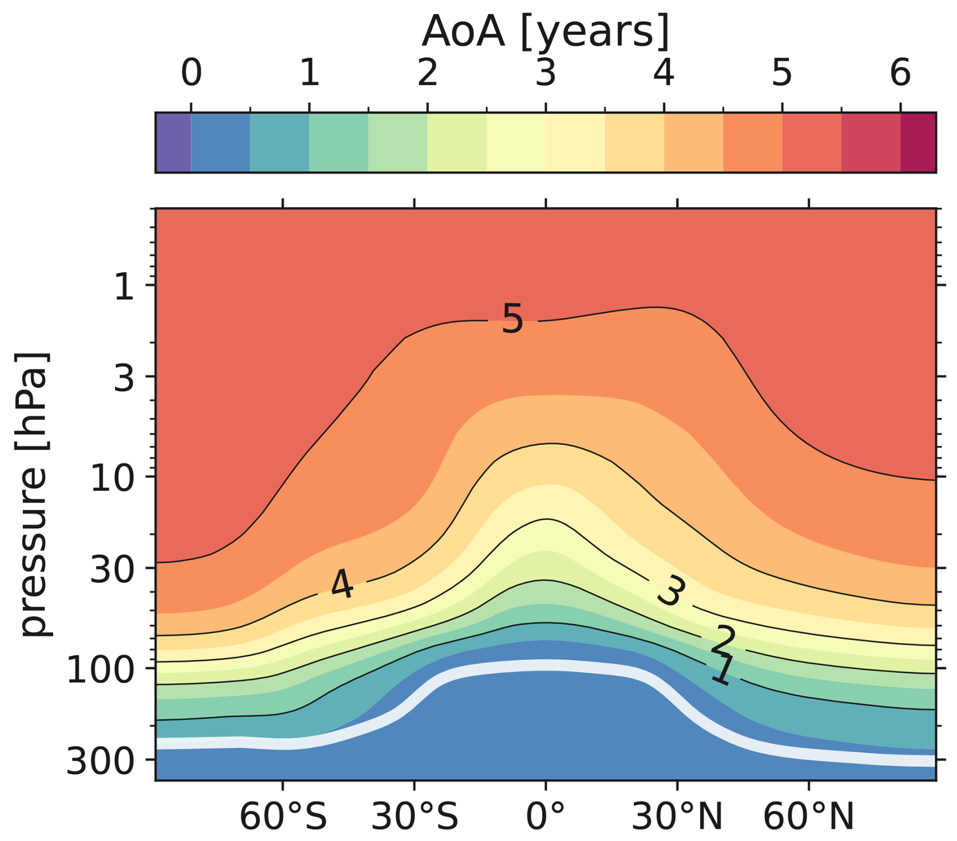
Figure 2 5-year average zonal-mean ensemble-mean AoA in the stratosphere for the CF ensemble, from 1 January 1994 to 1 January 1999, in years. The tropopause is plotted as a thick white line.

This age distribution is well within the intra-model spread derived from reanalyses, both by in-situ and offline transport models (Chabrillat et al., 2018; Ploeger et al., 2019; Fujiwara et al., 2022). It is also comparable to but slightly older than results from other coupled models simulating a similar historical period. For example, the E3SMv2-SPA mean age distribution is older than published results for the Whole Atmosphere Community Climate Model (WACCM) by up to ∼ 6 months (Garcia et al., 2011; Davis et al., 2023). This is primarily because those studies compute the AoA with respect to a reference point at the tropical tropopause, whereas our reference point is closer to the surface. We did not test this or perform a specific intercomparison, though we note that the 6-month contour in Fig. 2 correlates with the average position of the tropopause. The tropopause position is an E3SMv2-SPA output variable and is determined via the lapse rate tropopause definition of the World Meteorological Organization.

We now turn to the climatological tracer flux balance for the AoA. Figure 3 again shows the CF ensemble-mean AoA averaged over 1994–1999, as well as the RCTT over the same period, and the difference (AoA − RCTT). The residual circulation streamfunction is overplotted in each panel. In order to visualize the backward trajectory integration which computes the RCTT at each point in the meridional plane, Fig. 4 shows the 5-year mean trajectories, as well as the trajectories for the last month in the averaging period, December 1998, for a single CF ensemble member. The 1998 trajectories exhibit oscillations in the midlatitudes, which are imprints of the seasonal movement of the BDC. This seasonal signal is smoothed out in the time-averaged trajectories.

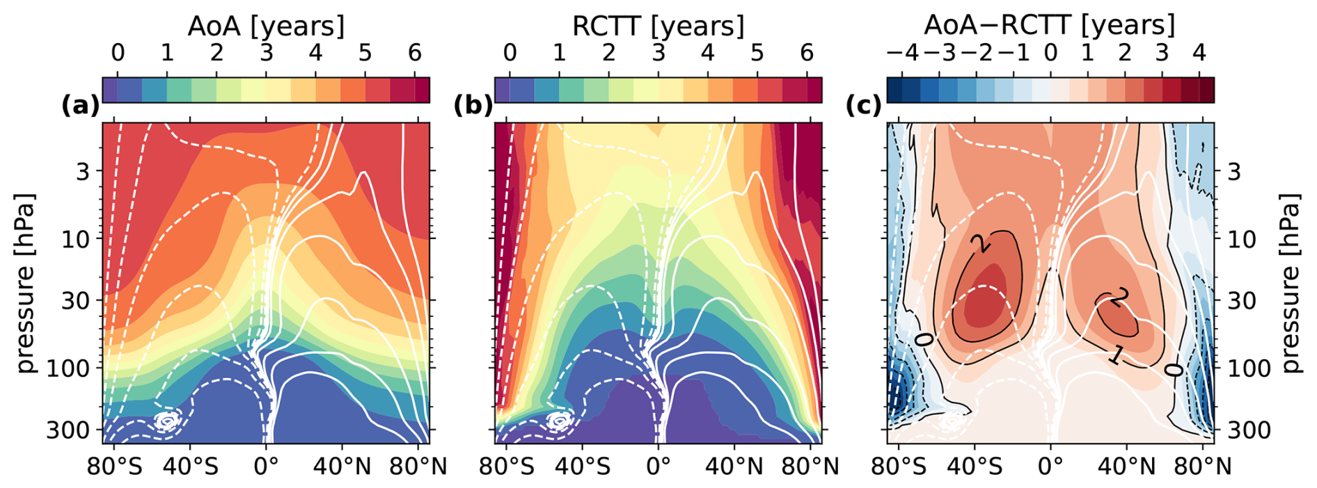
Figure 3 5-year mean CF ensemble mean of (a) the AoA, (b) the residual circulation transit time, and (c) their difference. Age contours are shown every 6 months, with years labeled in black in panel (c). Overplotted is the residual circulation streamfunciton in white contours at zero, and 3, 10, 30, 100, 300, and 1000 kg s⁻¹ on each side of zero, with negative contours are dashed.

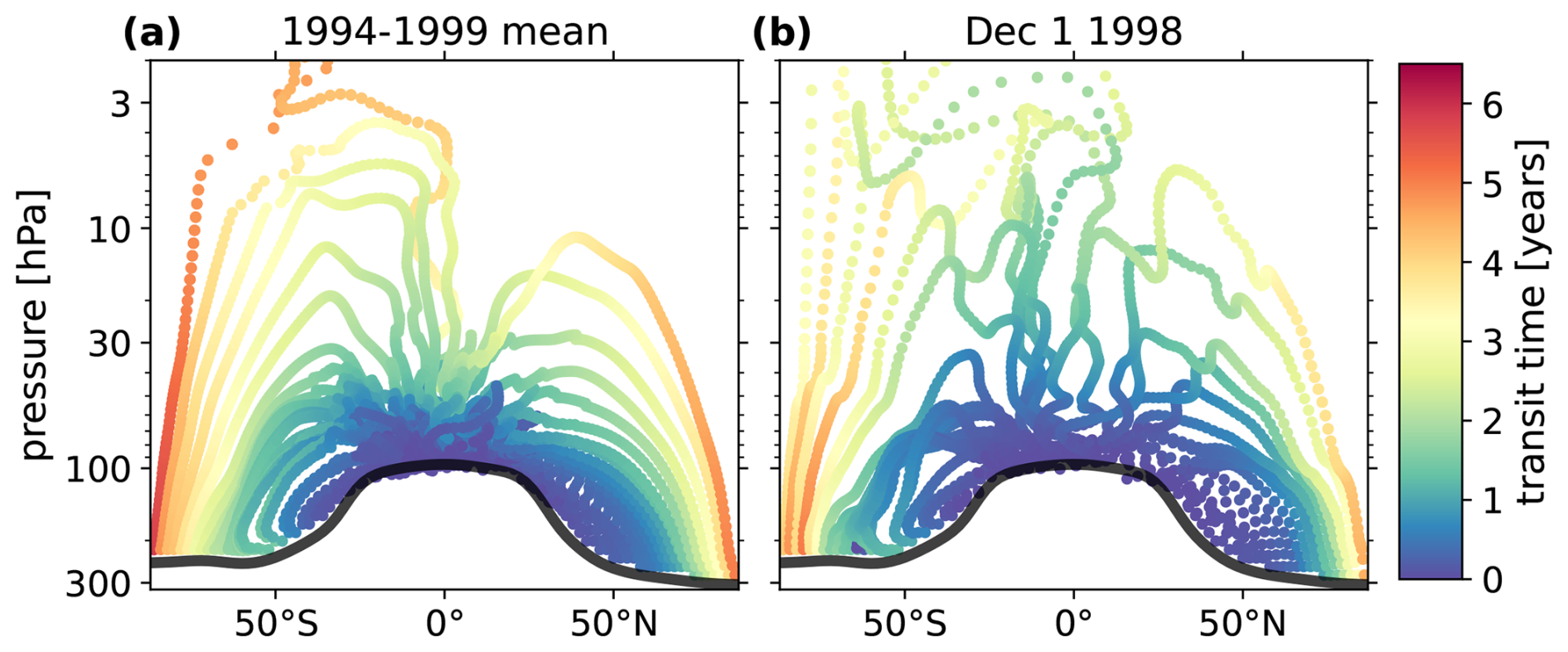
Figure 4 Select single-member (CF ensemble member 9) RCTT trajectories for gridpoints near the tropopause, every 2° in latitude, from 20–90° on each side of the equator. (a) the 5-year mean trajectories (b) the trajectories computed on 1 December 1998. The colors indicate the transit time along the trajectories. Note that visually discontinuous trajectories near the tropical tropopause are visible in panel (a). These features are an artifact of the trajectory averaging, due to the fact that the individual trajectories become highly variable in that region. These artifacts are not present in the individual member trajectories, and are purely visual, meaning that they do not affect the ensemble-mean RCTT in any way.

The RCTT in Fig. 3 shows the age due to advective residual circulation transport alone, which has a decreased vertical gradient in the tropics with respect to the AoA, and a much steeper meridional gradient in the midlatitudes. It appears that when wave-driven isentropic mixing is removed from the aging process, older and younger air are effectively segregated on either side of the surf zone. At 100 hPa, the mean age poleward and equatorward of 80° N is about 6 years and 3 years, respectively. Following Garny et al. (2014), we then interpret the difference in panel (c) as “aging by mixing”, i.e. aging that is not captured by the residual circulation advective transport. There are positive signals of up to 2.5 years of aging between 20–60° throughout the stratosphere in each hemisphere and negative signals of −4 years in the lower stratosphere at high latitudes. This difference, in principle, also includes any other parameterized transport or diffusion. However, Dietmüller et al. (2017) showed that these effects only comprise about 10 % of the net aging (or less) in their simulations. Thus, the primary mechanism is two-way exchange of old and young air across the meridional RCTT gradient by breaking resolved (Rossby) waves in the surf zone.

While the RCTT and its implied aging by mixing provide a view of the time-integrated tendencies along advective transport trajectories, further insight can be gained by instead considering local age tendencies. By “local”, we mean the instantaneous forcing imposed on the AoA in an Eulerian sense. For this, we recruit the TEM decomposition of the net age tendency, shown in Fig. 5. The panels show the (a) advection by the residual circulation (Eq. 5 plus Eq. 6), (b) local tracer mixing tendency by resolved waves (Eq. 11), (c) diffusion (Eq. 15), (d) sum of the resolved mixing and diffusion, and (e) net tendency, respectively. The data are averaged over the same 5-year time period as Fig. 3. The annual-mean AoA is very stable, and so the net tendency has been multiplied by a factor of 100 for visibility.

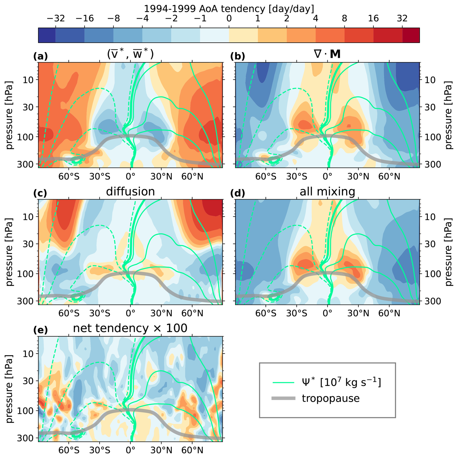
Figure 5 The 1994–1999 average TEM balance for the CF ensemble mean AoA. (a) advection by the residual circulation (b) mixing by resolved waves (c) mixing by diffusion (d) net mixing by resolved waves and diffusion (sum of panels b and c) (e) net tendency multiplied by 100. Overplotted in each panel is the tropopause in grey, and the residual circulation streamfunction in light green at 10, 70, and 300 on each side of zero in units of 10⁷ kg s⁻¹, with negative contours dashed.

Figure 5 tells the same story as Fig. 3, i.e. advection by the residual circulation decreases age in the tropics, and increases age poleward, peaking near the polar tropopause. The mixing tendency has the opposite behavior. At 100 hPa, the positive and negative diffusion signals peak near ±1 or less d d⁻¹, while the net mixing peaks in excess of ±4 d d⁻¹. Diffusion thus contributes at most 25 % of the mixing signal in the lower stratosphere, usually less. Above 30 hPa and poleward of 60° N, there are stronger diffusion contributions, which serve to nearly cancel large resolved mixing tendencies.

Note that the meridional position of the sign reversal in each of these quantities is located near 40° N, which is equatorward of the same feature as identified by the RCTT. To be clear, this difference is due to the local nature of the measurement; rather than being integrated, Fig. 5a shows the age by residual circulation advection given the simultaneous, pre-mixed AoA distribution.

Dietmüller et al. (2017) went on to show that one can obtain the cumulative effect of diffusion by integrating the resolved local mixing tendency (Fig. 5b) along RCTT backward-trajectories, and subtracting it from the RCTT–inferred mixing (Fig. 3c). We did not perform this calculation, but the relatively small local diffusion tendencies we see throughout the tropical column in Fig. 5c are consistent with the result of Dietmüller et al. (2017) that aging by diffusion is a secondary contribution.

The net tendency is much larger in seasonal averages than it is in the annual mean of Fig. 5e. Seasonal AoA TEM balances for winter and summer are provided in Appendix A, Figs. A1 and A2. The AoA tendency exhibits a seasonal signal, with enhanced aging occurring in the midlatitude winter hemisphere, and decreased negative aging shifted from the equator to 30° in the summer hemisphere. These effects are explained by the polar vortex-associated wave activity in the winter hemisphere (and lack of wave-driven mixing in the quiescent summer hemisphere), and the shift of the residual circulation streamfunction zero-line into the summer hemisphere. We note that these findings are consistent with Konopka et al. (2015), where a Lagrangian transport model driven by reanalysis winds was used to estimate the seasonality of the TEM AoA forcing.

5 Volcanic Impacts

With the mean and seasonal counterfactual behavior established for the AoA tracer, we now investigate the Mt. Pinatubo eruption impacts on the tracers and the force balance governing their evolution in the LV ensemble. First, it is useful to look at the volcanic effect on the residual circulation itself. It was noted in Part 1 that the most significant dynamical impacts on zonal momentum in the northern hemisphere occur during boreal summer 1991, late winter 1992, and summer 1992. Moreover, the primary impact driver was a strengthened residual circulation and the associated Coriolis effect during the boreal summer months, and modification of the EP flux divergence involving equatorward deflection of planetary waves near 30 hPa during the winter months. With this in mind, Fig. 6 shows the LV ensemble–mean $\mathrm{\Delta }{\stackrel{\mathrm{‾}}{w}}^{*}$ and ΔΨ^* averaged over August 1991, January 1992, and August 1992.

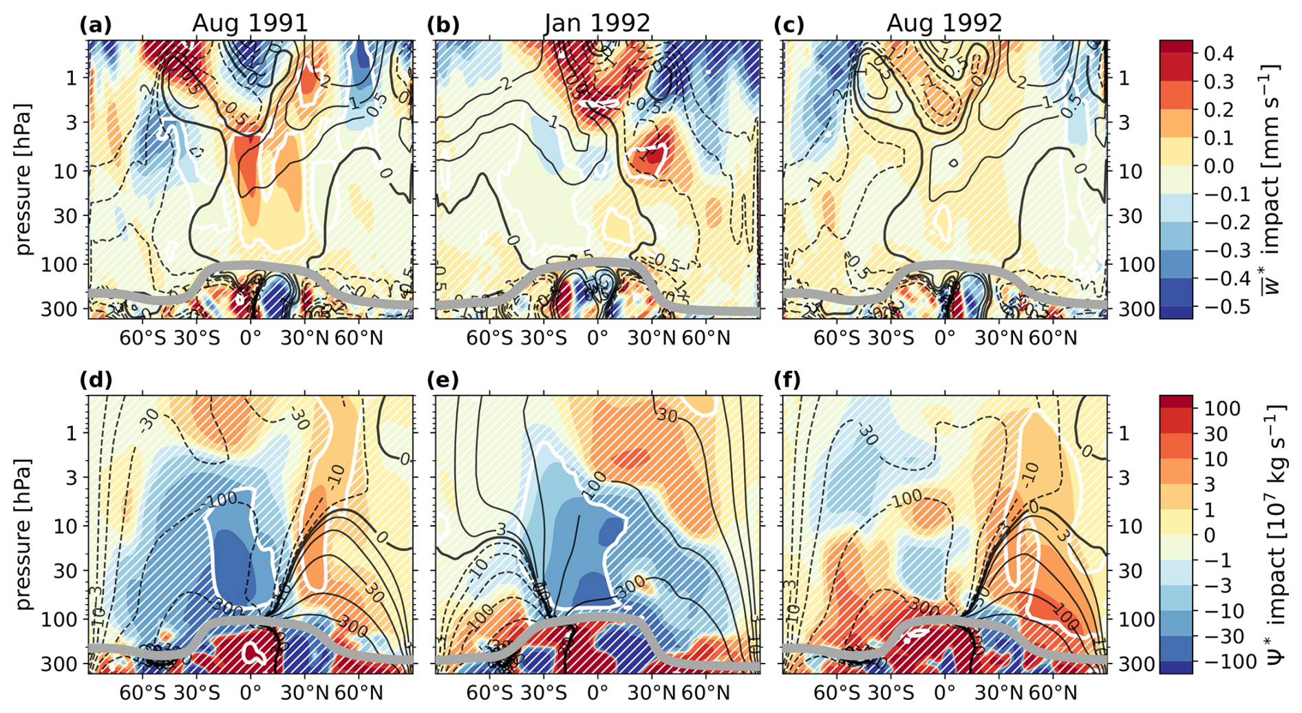
Figure 6 Ensemble-mean residual circulation impact, significance, and counterfactual reference for August 1991, January 1992, and August 1992. (a–c) the vertical residual velocity impact $\mathrm{\Delta }{\stackrel{\mathrm{‾}}{w}}^{*}$ in mm s⁻¹. A white contour is drawn at 95 % significance, and regions of insignificance are filled with white hatching. Overplotted in black contours is the CF ensemble-mean ${\stackrel{\mathrm{‾}}{w}}^{*}$ at 0.5, 1, and 2 mm s⁻¹ on each side of zero, with the zero line plotted in bold. (d–f) the residual streamfunction impact ΔΨ^* in 10⁷ kg s⁻¹. Significance is displayed as in panels (a)–(c). Overplotted in black contours is the CF ensemble mean Ψ^* at 3, 10, 30, 100, and 300 on each side of zero, in the same units, and the zero line plotted in bold.

In each of the seasons shown, there is enhanced residual (diabatic) vertical motion in the tropics, and enhanced downwelling in the high latitude upper stratosphere, though the strength and significance of these features are notably diminished by August of 1992, one year post-eruption. By continuity, this implies an accelerated residual circulation, which is observed in panels (d) and (f). In particular, the impact pattern indicates an enhanced overturning circulation centered on the aerosol forcing, which is near the injection latitude at 15° N in summer of 1991, and migrates poleward thereafter (Brown et al., 2024). The result is that the volcanic effect lacks the seasonality of the background residual circulation, and does not always project onto the CF Ψ^*. In August of 1991 and 1992, the robust ΔΨ^* indicates acceleration of the shallow branch of the BDC in both hemispheres, while the deep branch in the summer hemisphere is weakened. During January of 1992, the southern shallow-branch cell is enhanced along its northern edge, the Ψ^* zero line moves northward, and the positive overturning circulation in the SH is decelerated.

We found that the statistical significance of the residual velocity impacts extend to about 2 years post-eruption, after which the magnitude decreases and becomes statistically insignificant (not shown), which matches the timescale of the dynamical anomalies presented in Part 1. However, these relatively short–lived perturbations to the residual circulation are able to establish much more persistent changes to stratospheric composition, as indicated by the AoA.

5.1 AoA impacts

The AoA impact is shown for select monthly means and pressure levels between June 1991 and June 1998 in Fig. 7. Panels (d) and (e) show ΔAoA as a function of time and latitude at 10 and 30 hPa, respectively. Panels (a)–(c) show the monthly–averaged vertically–resolved impacts during boreal winter of 1992, 1993, and 1994. These monthly means were chosen as the occurrence of peak impact, the arrival of significant impact to the poles, and the initial return of the tropical AoA to the CF condition respectively, at 10 hPa.

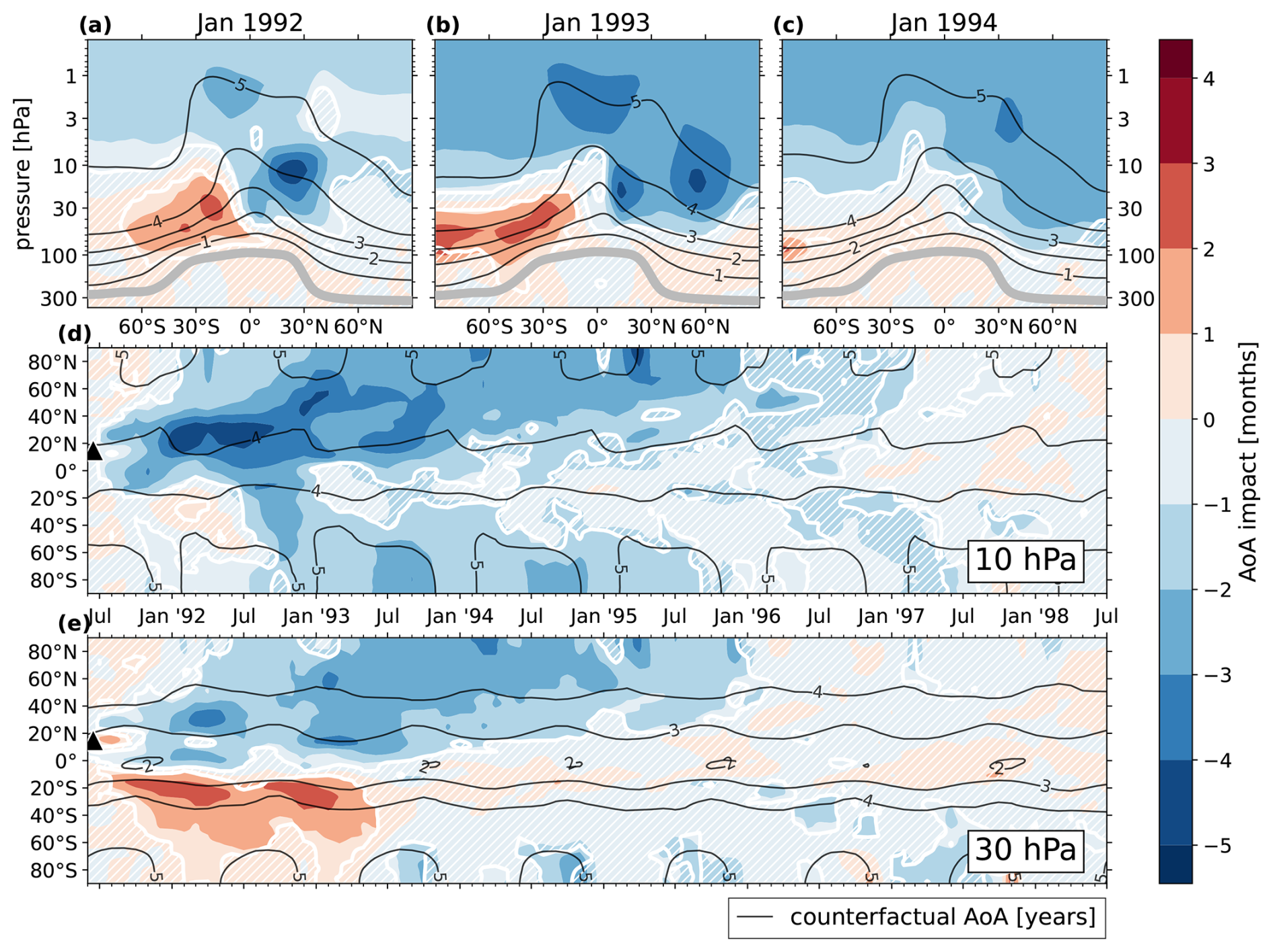
Figure 7 Ensemble–mean AoA impact, significance, and counterfactual reference for January 1992, January 1993, and January 1994. (a–c) the AoA impact in months. A white contour is drawn at 95 % significance, and regions of insignificance are filled with white hatching. Overplotted in black contours is the CF ensemble-mean AoA in years. (d) the same as panels (a)–(c), but for the time-latitude plane at 10 hPa (e) the same as panel (d), but at 30 hPa.

The ${\stackrel{\mathrm{‾}}{w}}^{*}$ impacts in Fig. 6 generally indicate an enhanced tropical pipe following the eruption, and as such the AoA signal is by-and-large an intrusion of younger air into the stratosphere. This feature migrates vertically and then poleward, which persists in significance for several years after the anomalous upwelling has ceased. The tropical impact diminishes from January 1993 to January 1994 at 10 hPa, while the impacts poleward of 60° N remain until at least 1996. This timescale can be thought of as the transit time of a “pulse” of young tropical air, and hence is itself a measurement of the BDC traversal timescale.

Also observed in panels (a)–(c) and (e) is a significant positive age anomaly in the SH between 30 and 100 hPa, lasting until July of 1993. We'll refer to this feature as SH lower stratosphere (SHLS) aging. Because the SHLS aging is a robust finding, and yet does not obviously follow from the expectation of an accelerated residual circulation, we will center the following discussion of the AoA flux balance on attributing its cause. This exercise should also provide insight into the volcanic aging process more generally. As a working hypothesis, the observation seems to be related to (1) the fact that ΔΨ^* does not project onto the CF Ψ^* in austral summer (Fig. 6e), and (2) the fact that the relatively slow migration of the AoA signal means that the interannual aging impact is dependent on the relatively early transport modification.

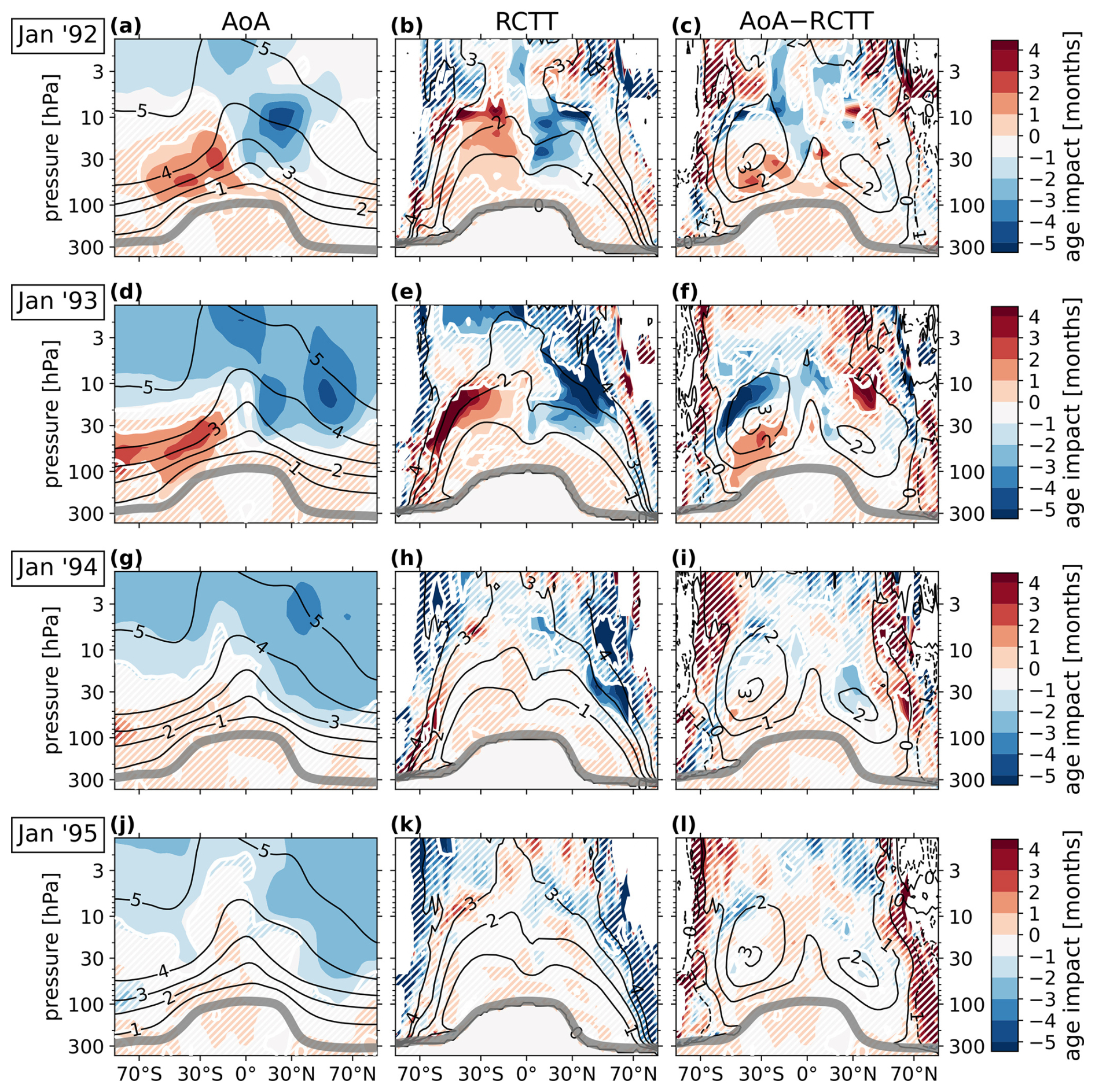
Figure 8 LV ensemble–mean aging impacts and their statistical significance in the total AoA (left column), the RCTT (middle column), and aging by mixing (right column) for Januarys from 1992–1995 (rows). In each panel, the CF ensemble mean of each age variable in years is plotted as labeled black contour. White contours are drawn at 95 % significance, and regions of insignificance are filled with white hatching. Solid white areas in the polar regions of the center and right column panels are missing–value locations where originating RCTT backward trajectories did not reach the tropopause within the integration domain.

Figure 8 shows ΔAoA, ΔRCTT, and their difference (aging by mixing) for boreal winters from 1991–1995. Panel (b) shows a robust symmetric signal about the equator, where air is refreshed in the NH subtropics, and aged SH subtropics by residual circulation advection. This transport anomaly explains most of the net aging signal (panel a). Visually scanning down panels (b), (e), (h), (k) shows that the RCTT impact in each hemisphere strengthens and advects along the residual circulation, following lines of constant transit time poleward.

In panels (d), (e), (f), the SHLS aging can be described by both enhanced advective transport and eddy tracer flux, though the impacts on each are larger than the net age increase. A momentum–based interpretation of this might be that the enhanced aging in the RCTT implies a decelerated residual circulation in the SH, which in turn implies accelerated summertime easterlies (decreased westerly Coriolis torque), and thus hampered diffusion, which approximately maintains thermal wind balance (see Part 1 for extended discussion on the utility of a thermal–wind–balance understanding of the volcanic response). Indeed, our results of Part 1 showed that residual circulation anomalies were usually associated with anomalous wave driving of approximately equal and opposite sign, and the net impact was a relatively small imbalance. From a tracer perspective, the equivalent statement is that enhanced aging by residual circulation advection (panel e SH) tends to be associated with decreased aging by mixing (corresponding feature in panel f). This cancellation (above 30 hPa) is achieved by a downward displacement of mixing contours, yielding an excess aging by mixing below the RCTT anomaly (below 30 hPa), which in part drives the net aging signal in panel (d). One possible physical interpretation of this feature is that as the circulation is perturbed, the critical level for propagating Rossby waves is altered. This would induce anomalous mixing through wave-breaking at the critical level, but also lead to further anomalous Lagrangian transport via the Stokes drift effect as the waves continue to propagate with perturbed amplitude.

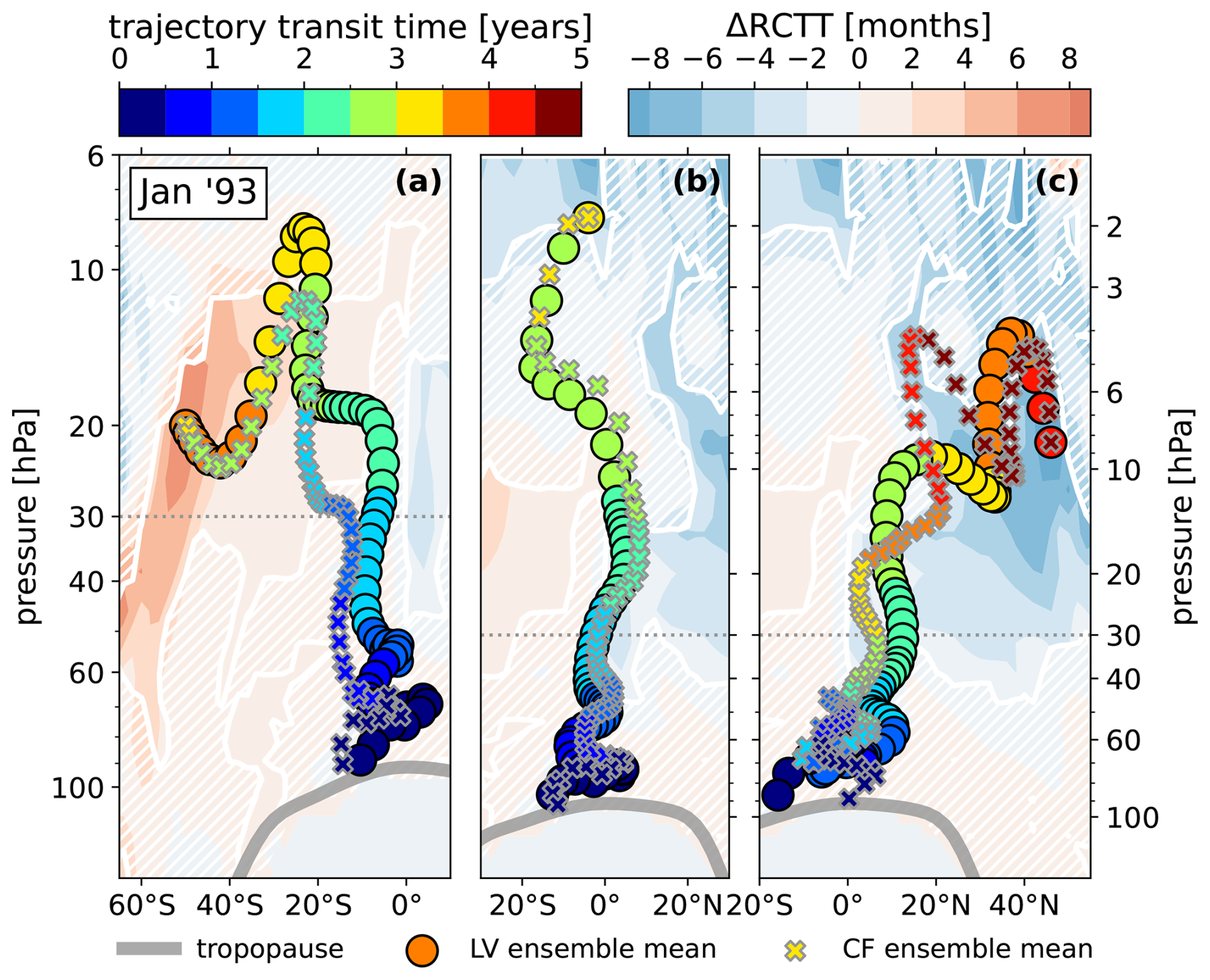
Figure 9 Comparison of select LV and CF ensemble-mean RCTT trajectories averaged over January of 1993. The trajectories were chosen as those corresponding to peak RCTT impact in (a) the midlatitude SH, (b) the tropics, and (c) the midlatitude NH. Colored points show the steps of the RK4 backward-integration of the time-varying residual velocity field (Sect. 3.3). Times on the top-left colorbar are reported as the difference between the trajectory launch time, and the tropopause intersection time. Circles and crosses are used for the LV and CF trajectories, respectively. Background colored contours show ΔRCTT, over which white contours are drawn at 95 % significance, and regions of insignificance are filled with white hatching. A faint dotted line is drawn at 30 hPa for reference. Panels (b) and (c) share a vertical axis.

Whatever the dynamical explanation of the advection-mixing balance at play here, it appears to be initiated by the anomalous vertical advection in the first place. Therefore, we will limit our present focus to an explanation of the anti–symmetric hemispheric signal in the RCTT at early times (as in Fig. 8b, e). Figure 9 reproduces the RCTT impacts for three overlapping latitude bands centered on the positive southern ΔRCTT feature, the equatorial region, and the negative northern ΔRCTT feature averaged over January 1993. For each region, a pair of CF and LV ensemble-mean RCTT trajectories are shown. The particular trajectories chosen are those that connect the tropopause to the peaks of significant ΔRCTT near (60° S, 20 hPa), (0°, 6 hPa), and (40° N, 10 hPa). The intention Fig. 9 is to clarify whether the difference in transit time are primarily due to difference in trajectory, or difference in transport speed.

We can see that while the trajectories are in fact different, their behavior is qualitatively comparable, and it seems that the more important effect is a difference in the background residual velocity, particularity ${\stackrel{\mathrm{‾}}{w}}^{*}$. In the SH (panel a), the total transit time lag is about 6 months, which is already established by the time the trajectories cross the 30 hPa isobar, before they turn southward toward their destination. A similar but opposite conclusion is reached for the NH trajectory (panel c), where the total lag of −8 months appears to have been reached by 30 hPa. The equatorial trajectory in panel (b) exhibits almost exclusively vertical motion, and reaches its destination with a lag of several months.

These findings reinforce one of our initial hypotheses, that relatively early transport anomalies, specifically $\mathrm{\Delta }{\stackrel{\mathrm{‾}}{w}}^{*}$, control the ultimate RCTT impact distribution. But the question remains as to why exactly the RCTT lag in each hemisphere is of opposite sign, if the fundamental effect is enhanced upwelling. To address this problem, Fig. 10 shows $\mathrm{\Delta }{\stackrel{\mathrm{‾}}{w}}^{*}$, ΔRCTT, and the impact in the local residual circulation flux as diagnosed by the advective TEM contribution (Eq. 5 plus Eq. 6) in the latitude-time plane at 30 hPa. Overplotted is the zero-line of the CF ensemble-mean ${\stackrel{\mathrm{‾}}{w}}^{*}$, with bold arrows indicating regions of upwelling and downwelling. Also shown is the position of the Mt. Pinatubo eruption, and the latitude of the maximum temperature impact ΔT.

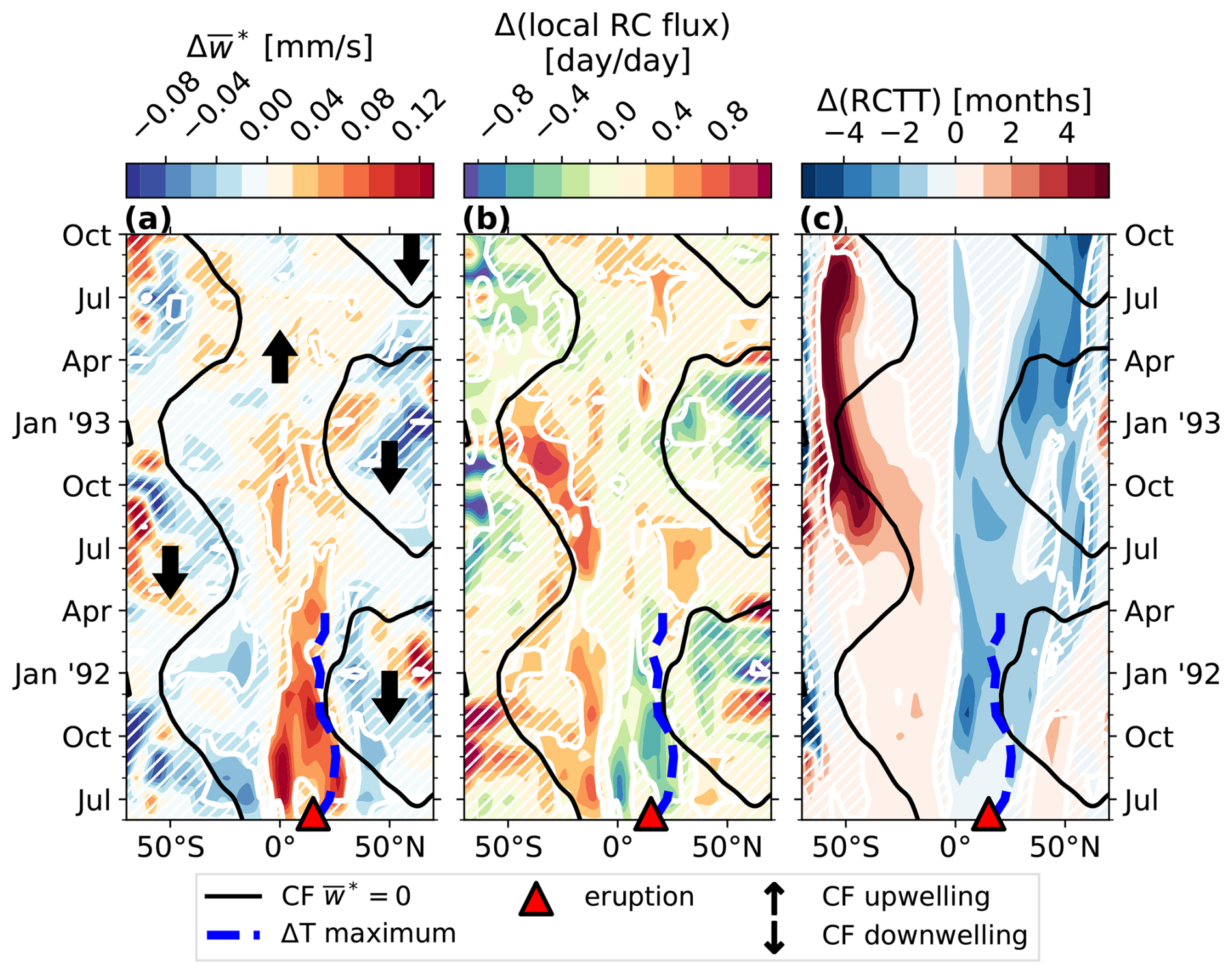
Figure 10 Relationship between the ensemble-mean impacts in vertical residual velocity, and aging by residual circulation advection at 30 hPa from July 1991 to October 1993. In all panels, solid black contours are drawn at ${\stackrel{\mathrm{‾}}{w}}^{*}=\mathrm{0}$ in the CF ensemble mean, a thick dashed blue line shows the latitude of maximum ΔT from July 1991 to April 1992, and a red triangle shows the position of the Mt. Pinatubo eruption. White contours are drawn at 95 % significance, and regions of insignificance are filled with white hatching. (a) $\mathrm{\Delta }{\stackrel{\mathrm{‾}}{w}}^{*}$ in mm s⁻¹. Thick black arrows show regions of upwelling and downwelling in the CF data. (b) impact in AoA local residual circulation advective flux (Eqs. 5 and 6) in d d⁻¹. (c) RCTT impact in months.

Now, wherever positive (negative) contours in $\mathrm{\Delta }{\stackrel{\mathrm{‾}}{w}}^{*}$ coincide with regions of upwelling (downwelling), the aerosol forcing is enhancing the local vertical motion, and thus the RCTT is decreased with respect to the counterfactual. This means that the robust $\mathrm{\Delta }{\stackrel{\mathrm{‾}}{w}}^{*}>\mathrm{0}$ (red) feature centered on the eruption latitude in panel (a) brings relatively young air into the upper stratosphere, as expected. On the other hand, when the signs of $\mathrm{\Delta }{\stackrel{\mathrm{‾}}{w}}^{*}$ and the CF ${\stackrel{\mathrm{‾}}{w}}^{*}$ are different, the opposite effect on the RCTT will result. Importantly, this means that the robust $\mathrm{\Delta }{\stackrel{\mathrm{‾}}{w}}^{*}<\mathrm{0}$ (blue) features south of the equator from July 1991 to April 1992 in panel (a) are acting to increase transit times through the vertical column aloft. This results in a concomitant increase in the local residual circulation advective flux (panel b), which necessarily gives rise to a delayed effect in the integrated measure ΔRCTT (panel c). In other words, the early negative upwelling impact in the southern subtropics releases a “pulse” of old air which remains robustly detected for several years as it traverses the BDC.

There are two effects which cause this particular response; (1) after the eruption occurs at 15° N, the maximum ΔT, and thus maximum $\mathrm{\Delta }{\stackrel{\mathrm{‾}}{w}}^{*}$, remains in the NH for at least one year at 30 hPa. By continuity, this must involve enhanced downwelling north and south of the forcing, which occurs north of 45° N and south of 0°. The result is anomalous upwelling and downwelling on opposite sides of the equator. (2) The seasonal shift of the BDC exacerbates this meridional asymmetry, since the region of upwelling (i.e. the diverging region of the residual streamfunciton) migrates into the southern hemisphere (black contours in panel a), which we saw in Fig. 6e. This means that the positive aging effects of the anomalously low vertical motion in this region is strengthened.

To be clear, if the eruption had instead occurred at the equator, the SHLS aging might still be observed due to the seasonal southern migration of the shallow BDC branches. If the eruption had instead occurred during boreal winter, then the seasonal BDC signal would be the opposite, and we would perhaps see aging in the NHLS instead. In any case, we have arrived at the second of our initial hypotheses, which was that the SHLS aging effect is a result of the misalignment of ΔΨ^* and the CF Ψ^*, though the eruption localization also plays a notable role. The essential mechanism is this; while the split between the BDC shallow branch cells exhibit a meridional oscillation, the volcanic forcing of the residual circulation in contrast is fixed near the eruption location, which alters the relative sign between $\mathrm{\Delta }{\stackrel{\mathrm{‾}}{w}}^{*}$ and ${\stackrel{\mathrm{‾}}{w}}^{*}$.

This “seasonal mechanism” also explains why the SHLS aging abruptly ends near July of 1993 (as seen in Fig. 7e). Note that the positive impacts on the local residual circulation flux in the SH of Fig. 10b are bound by the ${\stackrel{\mathrm{‾}}{w}}^{*}=\mathrm{0}$ line; these impacts arise during austral summer, and dissipate during austral winter as the meridional oscillation of the ${\stackrel{\mathrm{‾}}{w}}^{*}=\mathrm{0}$ line modulates the relative sign between $\mathrm{\Delta }{\stackrel{\mathrm{‾}}{w}}^{*}$ and ${\stackrel{\mathrm{‾}}{w}}^{*}$. This process repeats for as long as the volcanic forcing is significant, or about two years, after which the northward motion of the ${\stackrel{\mathrm{‾}}{w}}^{*}=\mathrm{0}$ line starting in January 1993 ushers out the roughly two-year-long era of diminished transport in the SHLS. This signal then arises as a delayed positive ΔRCTT, which itself ends equally as abruptly about nine months later.

Though this is perhaps a laborious explanation, it paints an elegant picture of the global driving force behind the hemispherically asymmetric response that was observed in our experiments. The proceeding Sect. 5.2 offers a cleaner interpretation of this identified mechanism, and the effects that it may have on the BDC seasonality more generally.

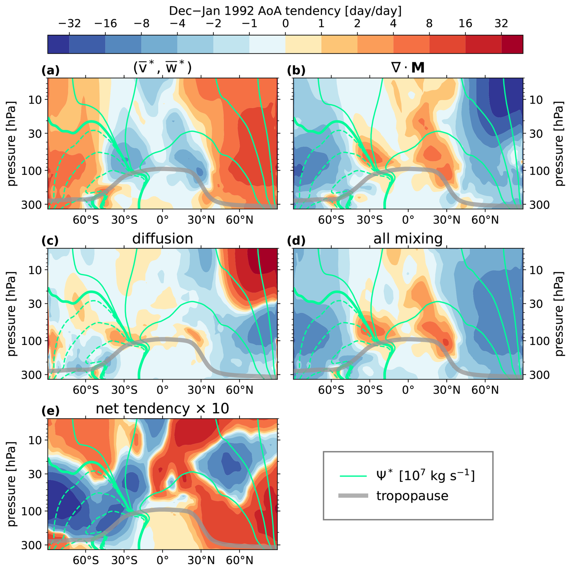
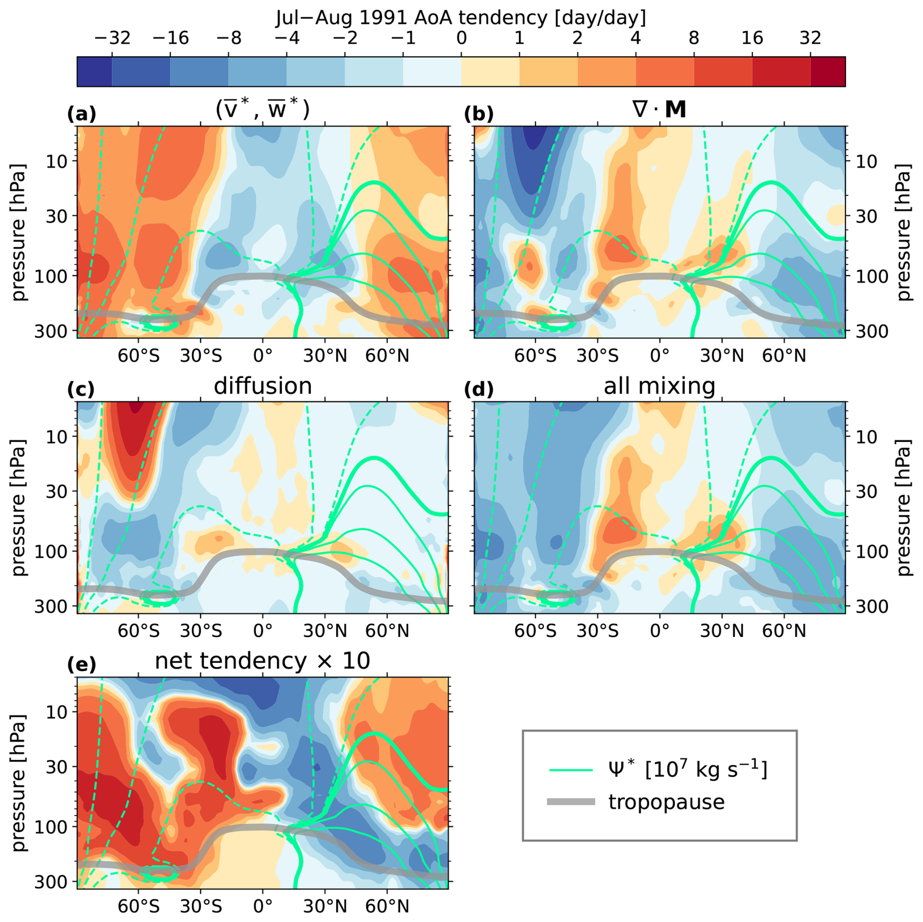
5.2 Effect on the BDC seasonality

With the volcanic effects on AoA reviewed, let us step back for a brief qualitative interpretation. We observed that a robust feature of increased age develops in the SHLS soon after the eruption, and ceases abruptly two years later. We noted that this is due in part to the occurrence of the eruption in the northern hemisphere, but that the effect is also controlled by the seasonal drift of the BDC with respect to the aerosol forcing, which modulates the relative sign between $\mathrm{\Delta }{\stackrel{\mathrm{‾}}{w}}^{*}$ and ${\stackrel{\mathrm{‾}}{w}}^{*}$.

A more general understanding can be gleaned from this collection of evidence, which is that tropical volcanic aerosol forcing occurring during a particular season tends to nudge stratospheric tracer transport tendencies toward that of the opposite season. This is seen explicitly in Fig. 11. Panel (b) shows the CF ensemble mean AoA tendency averaged over the summertime of 1991, and panel (c) shows the same for the wintertime. The opposite sign of the hemispheric asymmetry in these panels reflects the seasonal oscillation of the BDC circulation cells. Panel (a) shows the ensemble mean impact on the AoA tendency. A green contour showing the impact significance boundary is produced on all three panels for visual reference. By comparing the sign of the impact in the regions of significance to the signs of the seasonal CF means, it is clear that the volcanic effect is to oppose the transition from the summer to winter AoA distribution. For the full TEM budgets of the seasonal CF tendencies, see Figs. A2 and A1.

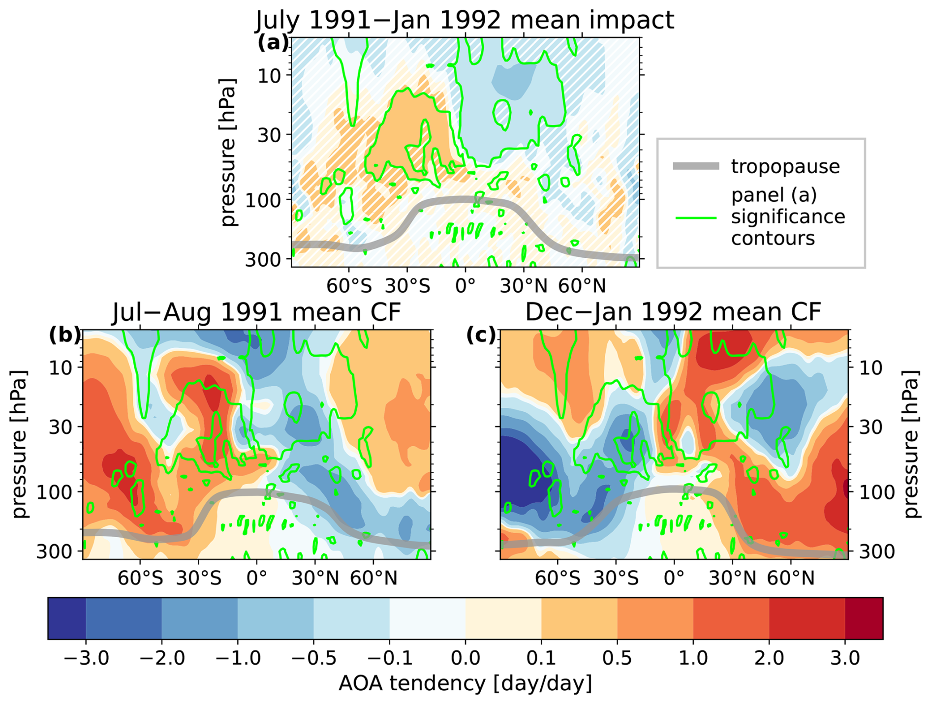
Figure 11 Indication of the hypothesized BDC seasonal cycle damping during the first 8 months of the volcanic experiments, in terms of the AoA tendency in d d⁻¹. (a) the ensemble-mean impact, averaged between 1 July 1991 and 1 January 1992. A green contour is drawn at 95 % significance, and regions of insignificance are filled with white hatching. (b) the summertime CF ensemble-mean, averaged between 1 July 1991 and 1 August 1991. (c) the wintertime CF ensemble mean, averaged between 1 December 1991 and 1 January 1992. In all panels, a thick grey line shows the tropopause averaged over the same period. In panels (b) and (c), the thin green significance contour from panel (a) is reproduced for visual reference.

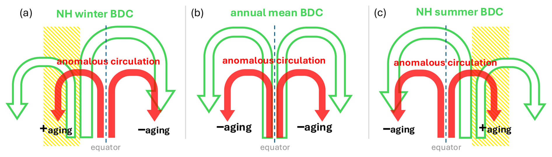
Figure 12 Schematic of the proposed BDC seasonal damping mechanism. Hollow green arrows represent the advective shallow BDC branches (Ψ^*) in the meridional plane, and solid red arrows represent the anomalous meridional residual circulation (ΔΨ^*) induced by a volcanic or similar forcing. Panels (a), (b), and (c) show the situation for boreal winter, the annual mean, and boreal summer, respectively. The sign of the resultant AoA impact is shown as “+aging” and “−aging”. Regions where $\mathrm{\Delta }{\stackrel{\mathrm{‾}}{w}}^{*}<\mathrm{0}<{\stackrel{\mathrm{‾}}{w}}^{*}$ (anomalous downwelling lies in a region of background upwelling) are filled with yellow hatching.

The net effect of this mechanism on the AoA is seen mainly in the SH in our experiments, since the Mt. Pinatubo eruption occurred in the NH. However, we hypothesize that the effect should be detectable in both hemispheres for a symmetric forcing. Considering other hypothetical Pinatubo-like eruptions occurring throughout the year, it appears that the generic effect on global mass transport of tropical eruptions is to dampen the seasonality of the BDC. A schematic of the hypothesized mechanism for a symmetric forcing source is shown in Fig. 12. The essential point is that the anomalous meridional circulation induced by the volcanic forcing (red arrows) only projects onto the background BDC in the annual mean (panel b). On seasonal timescales, the BDC oscillates, while the forcing instead evolves on much longer timescales (determined by the global transport of the volcanic sulfate aerosols). As a result the relative sign between Ψ^* and ΔΨ^*, as well as ${\stackrel{\mathrm{‾}}{w}}^{*}$ and $\mathrm{\Delta }{\stackrel{\mathrm{‾}}{w}}^{*}$ changes seasonally, which is illustrated as the yellow hatched regions of $\mathrm{\Delta }{\stackrel{\mathrm{‾}}{w}}^{*}<\mathrm{0}<{\stackrel{\mathrm{‾}}{w}}^{*}$ in Fig. 12. This is precisely the story told in Figs. 6, 10, and 11. Notice in particular that Fig. 12a corresponds qualitatively with Fig. 6e.

If this seasonal–damping mechanism is true, then it should be detectable by averaging the anomalous residual circulation and/or AoA over several years, given a steady and symmetric forcing source. The effect should also be accompanied by corresponding modifications to global EP flux divergence, which may in turn offer a more generalized interpretation of the results of Part 1. Future work could perhaps design simulated experiments toward this end. Experiments involving a more steady and symmetric forcing source, such as a simulated stratospheric aerosol injection (SAI), would lend themselves well to this inquiry. For the time being, we'd like to at least make one more incremental advance in the proceeding section, by inspecting the dependence of the BDC seasonal damping with the initial eruption size.

6 Eruption Magnitude Sensitivity

Thus far, we have not explored the sensitivity of our results to the forcing strength and instead limited our focus to a single volcanic scenario. This section provides a brief inspection of the qualitative relationship between the AoA tracer distribution and the initial eruption magnitude expressed in Tg of the aerosol precursor SO₂. As we have seen, the volcanic effect on global tracer concentrations is an indirect one, depending on interactions with the simultaneous background conditions. As such, it is difficult to make any a priori estimate of the trend. An idealized model of aerosol forcing as an exponential attenuation of longwave radiation (as in Hollowed et al. (2024)) suggests that the local heating rates should respond linearly at small mixing–ratio. However, we should not make the extrapolation that the local temperature response shares this scaling, let alone the nonlocal response after the downstream dynamical development.

Figure 13 shows the ΔAoA time series and eruption magnitude trend at 10 and 30 hPa averaged over 20–40° in each hemisphere. These positions were chosen to match the impact peaks in Fig. 7d, e. In the lower panels of Fig. 13a–d, the trend of the maximum $\left|\mathrm{\Delta }\mathrm{AoA}\right|$ is shown as a function of SO₂ mass, normalized such that the result for the 10 Tg eruption is set to unity. The maximum $\left|\mathrm{\Delta }\mathrm{AoA}\right|$ is identified uniquely for each SO₂ mass choice, and thus the occurrence of each in time are not always the same (marked with colored triangles in the figure). A linear fit to the normalized data is also shown for reference.

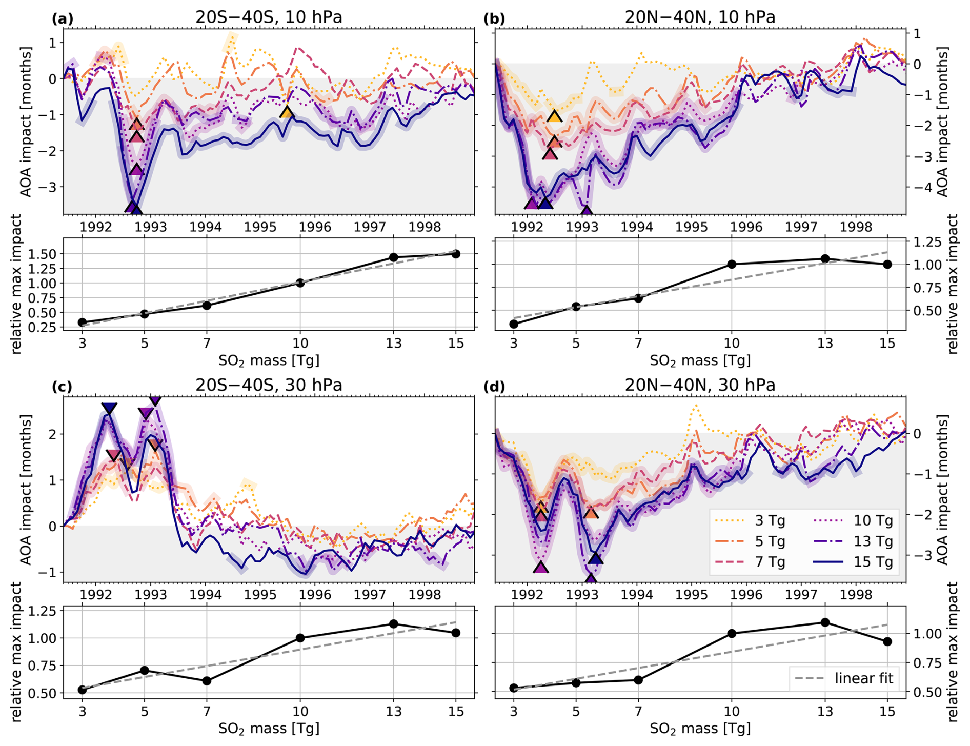
Figure 13 ΔAoA following eruptions with 3, 5, 7, 10, 13, and 15 Tg of eruptive SO₂. (a) top panel shows the ΔAoA time series at 10 hPa and averaged over 20–40°S for each eruption mass (legend in panel d). Each line is highlighted in color where the impact is statistically significant at the 95 % level. Bottom panel shows $\max \left(\right|\mathrm{\Delta }\mathrm{AoA}\left|\right)$, normalized such that the result for the 10 Tg eruption has a value of 1. Occurrence of the max impact is labeled in the top panel with a caret of matching color for each curve. A gray dashed line shows the linear fit to the data. (b, c, d) the same as panel (a), but for the pressure levels and meridional averaging as given in their titles above each top panel.

In the NH, the trend is approximately linear from 3 to 10 Tg, after which there is a hint of saturation in the ΔAoA from 10–15 Tg. The positive aging anomaly in the SH at 30 hPa qualitatively shows this effect as well, while at 10 hPa the trend is approximately linear from 3 to 15 Tg. Once the peak impacts are realized, panels (a), (b) and (d) suggest that larger anomalies also remain detectable for longer, as seen in the persistence of the significance of each impact curve with time. In panel (c), we see that the sudden drop in the SHLS aging occurs simultaneously for all eruption magnitudes, consistent with our earlier suggestion at the end of Sect. 5.1 that this behavior is controlled by the background BDC seasonal cycle.

The combination of Fig. 13c, d shows that both of the opposing southern and northern hemisphere responses scale together with eruption size, which implies that the seasonal damping effect on the BDC in general is linearly controlled over at least the tested forcing range. It is an open question whether or not the effect should saturate given even larger SO₂ loading. Either way, some nonlinear behavior should probably be expected, since the interaction between volcanic impacts and background dynamics could change approaching the condition $\left|\mathrm{\Delta }{\stackrel{\mathrm{‾}}{w}}^{*}\right|\approx \left|{\stackrel{\mathrm{‾}}{w}}^{*}\right|$.

7 Discussion and Conclusions

Our conclusions are as follows

1. The main effect of the Mt. Pinatubo eruption on tracer transport is to strengthen the tropical pipe, which lowers age of air throughout the tropics and in the middle-to-upper stratosphere globally.

2. Age impacts remain detectable long after the instigating dynamical perturbations have relaxed. They generally persist until they traverse the deep BDC (about 2 years in the tropics, and about 5 years at higher latitudes).

3. There is a hemispherically asymmetric response in the lower stratosphere, involving increased aging in the southern hemisphere, spanning one year post-eruption. We called this feature SHLS aging.

4. The SHLS aging is due to a combination of anomalous aging by both residual circulation advection and mixing.

5. The anomalous advective component of the SHLS aging is primarily attributed to vertical residual velocity impacts $\mathrm{\Delta }{\stackrel{\mathrm{‾}}{w}}^{*}$. The sign of the age impact in each hemisphere depends on the relative sign between $\mathrm{\Delta }{\stackrel{\mathrm{‾}}{w}}^{*}$ and the background condition ${\stackrel{\mathrm{‾}}{w}}^{*}$.

6. The relative sign between $\mathrm{\Delta }{\stackrel{\mathrm{‾}}{w}}^{*}$ and ${\stackrel{\mathrm{‾}}{w}}^{*}$ (or between ΔΨ^* and Ψ^*) is controlled by two properties: (1) meridional position of the eruption, and (2) the configuration of the lower branch of the BDC during the season following the eruption.

7. The generic interaction between tropical volcanic forcing and global tracer transport appears to be a damping of the BDC seasonal cycle, though this would need to be verified with additional studies.

Our interpretation of the BDC seasonal damping is an extrapolation from the observations presented here; while the finding in the SHLS is robust across the ensemble and also across the tested eruption magnitude range, it is limited to a single year and eruption location. Verification of this conclusion generically would be better suited to an experiment involving persistent and hemispherically symmetric aerosol forcing, rather than a transient and localized volcanic event. Fortunately, the plethora of simulated stratospheric aerosol injection (SAI) geoengineering experiments conducted during the past decade offer some insight. Bednarz et al. (2023) published a model intercomparison study of meridionally-varying aerosol injections, and concluded that ${\stackrel{\mathrm{‾}}{w}}^{*}$ anomalies are generally positive in the NH subtropics, and negative in the SH subtropics for injections near 15°. Notably, the negative anomalies in the SH occur north of the turn-around latitude (their Fig. 6). This resulted in excess concentrations of ozone in the SHLS in three out of four models they analyzed, consistent with our finding of increased AoA in that region (their Fig. 7). For the case of an equatorial injection, they showed positive anomalous upwelling near the equator, and downwelling poleward in each hemisphere, all of which occurred mostly within a region of climatological ${\stackrel{\mathrm{‾}}{w}}^{*}>\mathrm{0}$. Associated with this vertical motion effect was an ozone increase symmetric about the equator near 70 hPa.

Later, Henry et al. (2024) performed a similar series of SAI simulations with varying injection latitudes, and analyzed the resulting AoA anomalies (their Fig. 5). Consistent with Bednarz et al. (2023), they identified increases in aging of up to ∼3 months, near 70 hPa and within ±40° in latitude. They also reported AoA anomaly results from the ARISE-SAI-1.5 simulations (Richter et al., 2022; Henry et al., 2023). Those simulations included simultaneous injection locations at ±30 and ±15° in latitude, but with overall more SO₂ injected in the NH (see Henry et al. (2023) Fig. 2a). Consistent with both our work and Bednarz et al. (2023), for this scenario they identified AoA anomalies of nearly 3 months in the SHLS.

Though our results are consistent with the highlighted findings of Bednarz et al. (2023) and Henry et al. (2024), neither of those authors describe the aging effect in the lower stratosphere in terms of the BDC, saying instead that “The response results from local deceleration of upwelling in the tropical troposphere … brought about by the increase in static stability associated with heating in the lower stratosphere and cooling in the troposphere … This deceleration of tropospheric upwelling slows down the transport of ozone-poor tropospheric air into the lower stratosphere, thus increasing ozone in the region.” (Bednarz et al., 2023). This is perhaps at odds with our findings, since we observe robust SHLS aging despite the fact that the tropospheric vertical velocity impacts are not significant (Fig. 6a–c), though admittedly we did not pay special attention to the troposphere and did not plot $\mathrm{\Delta }{\stackrel{\mathrm{‾}}{w}}^{*}$ below 400 hPa. If there is a contribution from negative stratospheric ${\stackrel{\mathrm{‾}}{w}}^{*}$ anomalies to the lower stratosphere increases in age and ozone in Bednarz et al. (2023) and Henry et al. (2023), then it is also unclear if the seasonal effect that we have proposed here is contributing to the hemispherically symmetric response that they demonstrated for equatorial injections. In particular, they did not consider the meridionally-resolved time series of the response, which might have clarified the seasonal contributions to the long-time mean of their tracers. We hypothesize that their symmetric aging in the subtropical lower stratosphere is an average of SHLS aging in austral winter, and NHLS aging in boreal winter, which would be consistent with our conclusions.

In terms of volcanic eruption simulations, there are several works which support our findings. Pitari et al. (2016) used a paired–ensemble strategy similar to ours, and showed that changes of up to 0.1 mm s⁻¹ in ${\stackrel{\mathrm{‾}}{w}}^{*}$ follow the eruption of Mt. Pinatubo averaged on ±20° at 30 hPa. In latitude, the positive ${\stackrel{\mathrm{‾}}{w}}^{*}$ anomaly peaked near 10° N, and became negative at 10° S and 30° N. This is most likely consistent with our finding that the residual streamfunction anomaly does project onto the background condition during the summer of the eruption (Fig. 6d). They further showed that tropical and northern subtropical AoA decreased by several months, as well as the meridional age gradient. They did not show changes in age below 30 hPa, and so they may or may not have simulated the SHLS aging. Toohey et al. (2014) looked at the circulation response to the Mt. Pinatubo eruption with a 64–member ensemble, composed of four sets of 16 simulations, which averaged over different prescribed forcing datesets. They observed that the residual circulation averaged over boreal winter of 1991 was accelerated between 0 and 60° N below 1 hPa, and decelerated in the SH between 0 and 50° S (their Fig. 10f), the latter of which is consistent with our Fig. 6e.

A future study could be designed to test our seasonal BDC hypothesis more specifically, by simulating similar volcanic eruptions occurring at different latitudes and/or seasons, or by studying the meridionally– and vertically–resolved temporal evolution of residual circulation anomalies in SAI simulations. There could be any number of other variables to consider as well. An aspect that we did not discuss here is whether the phase of the quasi-biennial (QBO) complicates a potential interaction between volcanic forcing and BDC seasonality. A hint of this complication is found in Brown et al. (2023), who showed that the global symmetry of the post-eruption vertical velocity response depended strongly on the simultaneous QBO phase for equatorial eruptions in their simulations (their Fig. 10). It would also be enlightening to understand how exactly wave activity balances (or fails to balance) the global residual circulation response, which we only described in a more local sense in Part 1. Finally, there may be interest in exploring the sensitivity in the age impacts analyzed here to the SO₂ injection altitude, which was recently shown by Toohey et al. (2025) to strongly control to the aerosol lifetime (and thus forcing timescale) in the stratosphere.

Appendix A: Seasonal Tracer TEM Balance

This Appendix provides the seasonal TEM balance for the time tendencies of the age of air tracer. The winter and summer AOA forcing terms are shown in Figs. A1 and A2. See Sect. 4 for further discussions of the annual mean.

Figure A1 The same as Fig. 5, but for a winter climatological average.

Figure A2 The same as Fig. 5, but for a summer climatological average.