Technical note: Quantifying the nitrogen isotope difference between ammonium in the atmosphere and ammonia emitted from sources

The difference (δ¹⁵N_4a-3s) in nitrogen isotopes (δ¹⁵N) between NH${}_{\mathrm{4}}^{+}$ and source-emitted NH₃ is a crucial factor influencing the source apportionment of atmospheric NH${}_{\mathrm{4}}^{+}$. This δ¹⁵N_4a-3s is mainly due to isotopic fractionation during NH₃-NH${}_{\mathrm{4}}^{+}$ gas-particle conversion and atmospheric deposition. The impact of isotope fractionation on δ¹⁵N_4a-3s had been well quantified by simplified method, but that of atmospheric deposition had often been overlooked. This study developed a model to assess δ¹⁵N_4a-3s variations by considering both the atmospheric deposition and isotope fractionation. The results of six model scenarios showed the difference between δ¹⁵N_4a-3s values under both influences and under isotope fractionation alone increased with the rise of f (the molar fraction of NH${}_{\mathrm{4}}^{+}$ to NH_x in the atmosphere). At 20 °C, when f=0.9, the maximum gap could reach 10.7 %. δ¹⁵N_4a-3s was insensitive to NH₃ and NH${}_{\mathrm{4}}^{+}$ deposition ratio, NH${}_{\mathrm{4}}^{+}$ generation ratio, and temperature, but it was sensitive to f. A prediction function for δ¹⁵N_4a-3s was constructed and applied to atmospheric NH${}_{\mathrm{4}}^{+}$ source apportionment in the Yellow River Delta and Changsha. Compared with the simplified method, the fitted equation provided a more reasonable estimate of the contribution of agricultural sources and non-fossil fuel sources. The constructed equation could be used for tracing atmospheric NH${}_{\mathrm{4}}^{+}$ origin, thus improving the accuracy of atmospheric NH${}_{\mathrm{4}}^{+}$ source apportionment.

1 Introduction

Ammonia (NH₃) is the primary alkaline gas in the atmosphere, and its cycle plays a crucial role in the geological and biological nitrogen cycles on Earth's surface. NH₃ can neutralize atmospheric acids such as sulfuric acid (H₂SO₄), nitric acid (HNO₃), and hydrochloric acid (HCl), forming particulate ammonium (NH${}_{\mathrm{4}}^{+}$) aerosols. This process deteriorates air quality and affects the acidity of airborne particulate matter, precipitation, and cloud water (Ianniello et al., 2010; Pan et al., 2016; Chang et al., 2019b). NH₃ and NH${}_{\mathrm{4}}^{+}$ (collectively abbreviated as NH_x) are deposited back to the surface through dry and wet deposition processes. Excess NH_x in the atmosphere not only leads to eutrophication of terrestrial and aquatic ecosystems and threatens biodiversity, but also increases public health risks (Bobbink et al., 2010; Liu et al., 2019; Tan et al., 2020; Bouwman et al., 2002). In recent decades, rapid industrialization, urbanization, and agricultural development have significantly increased NH₃ emission worldwide, particularly in Asia, Africa, and South America. This resulted in a substantial rise in severe haze events and eutrophication risks in these regions (Zhao et al., 2017; Bouwman et al., 2002; Kim et al., 2011). In order to develop effective strategies to reduce NH_x levels in the atmosphere, source apportionment of NH_x has garnered considerable attention as a foundational research focus in recent years (Behera et al., 2013; Shen et al., 2011; Hu et al., 2014; Schiferl et al., 2016; Sun et al., 2016).

Numerous methods have been developed and used to trace sources of NH_x in the atmosphere. Among these, the utilization of the stable nitrogen isotopic composition of gaseous NH₃ (δ¹⁵N-NH₃) or aerosol NH${}_{\mathrm{4}}^{+}$ (δ¹⁵N-NH${}_{\mathrm{4}}^{+}$) has emerged as a highly promising tool for source apportionment of NH₃ in the atmosphere (Gu et al., 2025; Elliott et al., 2019). However, it is important to note that neither aerosol δ¹⁵N-NH${}_{\mathrm{4}}^{+}$ nor gaseous δ¹⁵N-NH₃ can be directly used for this purpose alone. This is because their isotopic values do not correspond directly to the δ¹⁵N-NH₃ of mixed NH₃ emissions from various sources (Zhang et al., 2020). The discrepancy arises from nitrogen isotope exchange between NH₃ and NH${}_{\mathrm{4}}^{+}$ in the atmosphere (Walters et al., 2019; Kawashima and Ono, 2019). Observations typically show higher δ¹⁵N values in NH${}_{\mathrm{4}}^{+}$ compared to NH₃, which can be attributed to equilibrium isotopic fractionation (Walters et al., 2019). The mass and isotope balance for NH_x in the atmosphere is given by the following equation:

$$\begin{array}{}\text{(1)}& f{\mathit{\delta }}^{\mathrm{15}}\mathrm{N}\text{-}{\mathrm{NH}}_{\mathrm{4}}^{+}+\left(\mathrm{1}-f\right){\mathit{\delta }}^{\mathrm{15}}\mathrm{N}\text{-}{\mathrm{NH}}_{\mathrm{3}}={\mathit{\delta }}^{\mathrm{15}}\mathrm{N}\text{-}{\mathrm{NH}}_x,\end{array}$$

where f is the molar fraction of NH${}_{\mathrm{4}}^{+}$ to NH_x in the atmosphere, and δ¹⁵N-NH${}_{\mathrm{4}}^{+}$, δ¹⁵N-NH₃ and δ¹⁵N-NH_x are the isotopic composition of NH${}_{\mathrm{4}}^{+}$, NH₃ and NH_x in the atmosphere, respectively. After the introduction of the isotopic fractionation factor (α) between NH${}_{\mathrm{4}}^{+}$ and NH₃, the Eq. (1) can be rewritten as:

$$\begin{array}{}\text{(2)}& \begin{array}{rl}{\mathit{\delta }}^{\mathrm{15}}\mathrm{N}\text{-}{\mathrm{NH}}_{\mathrm{4}}^{+}& ={\displaystyle \frac{\mathit{\alpha }}{\mathrm{1}+\left(\mathit{\alpha }-\mathrm{1}\right)f}}{\mathit{\delta }}^{\mathrm{15}}\mathrm{N}\text{-}{\mathrm{NH}}_x\\ & +{\displaystyle \frac{\mathrm{1000}\left(\mathit{\alpha }-\mathrm{1}\right)\left(\mathrm{1}-f\right)}{\mathrm{1}+\left(\mathit{\alpha }-\mathrm{1}\right)f}},\end{array}\end{array}$$

Because the coefficients of $\frac{\mathit{\alpha }}{\mathrm{1}+\left(\mathit{\alpha }-\mathrm{1}\right)f}$ and $\mathrm{1}+\left(\mathit{\alpha }-\mathrm{1}\right)f$ are approximately equal to one, the Eq. (1) is often simplified as:

$$\begin{array}{}\text{(3)}& \begin{array}{rl}{\mathit{\delta }}^{\mathrm{15}}{N}_{\text{4a-3x}}& ={\mathit{\delta }}^{\mathrm{15}}\mathrm{N}\text{-}{\mathrm{NH}}_{\mathrm{4}}^{+}-{\mathit{\delta }}^{\mathrm{15}}\mathrm{N}\text{-}{\mathrm{NH}}_x\\ & =\mathrm{1000}(\mathit{\alpha }-\mathrm{1})(\mathrm{1}-f),\end{array}\end{array}$$

where δ¹⁵N_4a-3x is difference between δ¹⁵N-NH${}_{\mathrm{4}}^{+}$ and δ¹⁵N-NH_x in the atmosphere. The difference is often used to correct the δ¹⁵N of NH${}_{\mathrm{4}}^{+}$ in the atmosphere, so as to apportion sources of NH${}_{\mathrm{4}}^{+}$ (Pan et al., 2018, 2016; Chang et al., 2016). The underlying assumption is that the atmosphere is a well-mixed closed system, implying that δ¹⁵N-NH_x values in the atmosphere are equivalent to those of the δ¹⁵N-NH₃ emitted from various sources. However, it is a well-established fact that both NH₃ and NH${}_{\mathrm{4}}^{+}$ can exit the atmosphere through deposition processes. These deposition processes may introduce substantial discrepancies between the δ¹⁵N-NH_x values observed in the atmosphere and the δ¹⁵N-NH₃ values emitted from sources. This bias could further compromise the accuracy of δ¹⁵N-based source apportionment (Zhang et al., 2020).

To more accurately identify the source of atmospheric NH_x, this study develops a model to quantify the difference in δ¹⁵N-NH${}_{\mathrm{4}}^{+}$ in the atmosphere and source-emitted δ¹⁵N-NH₃ (δ¹⁵N_4a-3s) under combined atmospheric deposition and isotope fractionation. It should be noted that the model primarily addresses the isotopic mass balance shift induced by deposition processes, rather than detailed chemical mechanisms. The objectives of this study are (1) to understand the variation pattern of δ¹⁵N_4a-3s and the key influencing factors, (2) to construct a fitting equation for the δ¹⁵N_4a-3s and the key influencing factors used for NH${}_{\mathrm{4}}^{+}$ source apportionment, and (3) to evaluate the application effects of the fitted equation in the source apportionment of NH${}_{\mathrm{4}}^{+}$ through practical examples.

2 Methods and Theory

2.1 Model Development

Similar to the Eq. (3), the δ¹⁵N_4a-3s could be calculated as follows:

$$\begin{array}{}\text{(4)}& \begin{array}{rl}{\mathit{\delta }}^{\mathrm{15}}{N}_{\text{4a-3s}}& =\left({\mathit{\delta }}^{\mathrm{15}}\mathrm{N}\text{-}{\mathrm{NH}}_{\mathrm{4}}^{+}-{\mathit{\delta }}^{\mathrm{15}}\mathrm{N}\text{-}{\mathrm{NH}}_{\mathrm{3}s}\right)\\ & =\mathrm{1000}\left(\mathit{\alpha }-\mathrm{1}\right)\left(\mathrm{1}-f\right),\end{array}\end{array}$$

where δ¹⁵N-NH_3s is the nitrogen isotope of NH₃ from various types of sources and other items are the same as that in Eqs. (1) and (2). The equation indicates that the variation in δ¹⁵N_4a-3s depends on the change of α, f and δ¹⁵N-NH_x. Consequently, the core objective of this model is to iteratively update α, f and δ¹⁵N-NH₃ in an open system that accounts for the combined effects of ${\mathrm{NH}}_{\mathrm{3}}/{\mathrm{NH}}_{\mathrm{4}}^{+}$ conversion and sedimentation, and ultimately to determine the steady-state δ¹⁵N_4a-3s.

Firstly, the parameter α is defined as $({\mathit{\delta }}^{\mathrm{15}}\mathrm{N}\text{-}{\mathrm{NH}}_{\mathrm{4}}^{+}+\mathrm{1000})/({\mathit{\delta }}^{\mathrm{15}}\mathrm{N}\text{-}{\mathrm{NH}}_{\mathrm{3}}+\mathrm{1000})$ (Coplen, 2011). This value of α could be empirically determined by fitting experimental data (Urey, 1947; Li et al., 2012) and computational quantum chemistry method (Walters et al., 2019) based on the ambient temperature. The present study used the computational quantum chemistry method (Walters et al., 2019) to calculate the α values as the following method:

$$\begin{array}{}\text{(5)}& \mathrm{1000}\left(\mathit{\alpha }-\mathrm{1}\right)={\displaystyle \frac{\mathrm{12}\mathrm{522}}{T\left(\mathrm{K}\right)}}-\mathrm{11.31},\end{array}$$

where T is the ambient temperature (in Kelvin). The values of f and δ¹⁵N-NH_x vary synchronously during the iteration. Next, the continuous variations in atmospheric NH₃ and NH${}_{\mathrm{4}}^{+}$, together with their deposition processes, were discretized. Assuming the atmosphere is a well-mixed open system, three processes occur simultaneously at each iteration step: partial conversion of NH₃ to NH${}_{\mathrm{4}}^{+}$, deposition loss of NH₃, and deposition loss of NH${}_{\mathrm{4}}^{+}$. Accordingly, the mass fractions of atmospheric NH₃ and NH${}_{\mathrm{4}}^{+}$, as well as their deposited fractions, can be expressed as follows:

$$\begin{array}{}\text{(6)}& \begin{array}{ll}& {\left[{\mathrm{NH}}_{\text{3a}}\right]}^t=\left(\mathrm{1}-G_{\mathrm{4}}-D_{\mathrm{3}}\right){\left[{\mathrm{NH}}_{\text{3a}}\right]}^{t-\mathrm{1}}\\ & {\left[{\mathrm{NH}}_{\text{4a}}^{+}\right]}^t=G_{\mathrm{4}}{\left[{\mathrm{NH}}_{\text{3a}}\right]}^{t-\mathrm{1}}+\left(\mathrm{1}-D_{\mathrm{4}}\right){\left[{\mathrm{NH}}_{\text{4a}}^{+}\right]}^{t-\mathrm{1}}\\ & {\left[{\mathrm{NH}}_{\text{3d}}\right]}^t=D_{\mathrm{3}}{\left[{\mathrm{NH}}_{\text{3a}}\right]}^{t-\mathrm{1}}\\ & {\left[{\mathrm{NH}}_{\text{4d}}^{+}\right]}^t=D_{\mathrm{4}}{\left[{\mathrm{NH}}_{\text{4a}}^{+}\right]}^{t-\mathrm{1}}\end{array},\end{array}$$

where G₄, D₃ and D₄ represent the transformation ratio of NH₃ to NH${}_{\mathrm{4}}^{+}$, and the deposition ratio of NH₃ and the deposition ratio of NH${}_{\mathrm{4}}^{+}$, respectively. All three are dimensionless parameters defined for a single iteration step. The superscript t denotes the iteration index, starting from t=1, and does not represent a specific physical duration. The model is iterated to steady state, and the resulting steady-state δ¹⁵N_4a-3s is taken as the model output. [NH_3a] and [NH${}_{\text{4a}}^{+}$] are the mass fractions of atmospheric NH₃ and NH${}_{\mathrm{4}}^{+}$, whereas [NH_3d] and [NH${}_{\text{4d}}^{+}$] are the corresponding deposited fractions in that iteration step. The molar fraction of NH${}_{\mathrm{4}}^{+}$ in NH_x at iteration step t can then be calculated as follows:

$$\begin{array}{}\text{(7)}& f^t={\displaystyle \frac{{\left[{\mathrm{NH}}_{\text{4a}}^{+}\right]}^t}{{\left[{\mathrm{NH}}_x\right]}^t}}={\displaystyle \frac{{\left[{\mathrm{NH}}_{\text{4a}}^{+}\right]}^t}{{\left[{\mathrm{NH}}_{\text{4a}}^{+}\right]}^t+{\left[{\mathrm{NH}}_{\text{3a}}\right]}^t}},\end{array}$$

where [NH_x]^t is the mass fraction of NH_x in the atmosphere at the tth time interval, and the meanings of other items are the same as those in Eq. (6). Furthermore, given that α and f are known, the values of [δ¹⁵N-NH${}_{\mathrm{4}}^{+}$] and [δ¹⁵N-NH₃] at the tth time interval can be expressed as:

$$\begin{array}{}\text{(8)}& \begin{array}{rl}& {\left[{\mathit{\delta }}^{\mathrm{15}}\mathrm{N}\text{-}{\mathrm{NH}}_{\text{4a}}^{+}\right]}^t={\left[{\mathit{\delta }}^{\mathrm{15}}\mathrm{N}\text{-}{\mathrm{NH}}_x\right]}^{t-\mathrm{1}}+\mathrm{1000}\left(\mathit{\alpha }-\mathrm{1}\right)\left(\mathrm{1}-f^{t-\mathrm{1}}\right)\\ & {\left[{\mathit{\delta }}^{\mathrm{15}}\mathrm{N}\text{-}{\mathrm{NH}}_{\text{3a}}\right]}^t={\left[{\mathit{\delta }}^{\mathrm{15}}\mathrm{N}\text{-}{\mathrm{NH}}_x\right]}^{t-\mathrm{1}}-\mathrm{1000}\left(\mathit{\alpha }-\mathrm{1}\right)f^{t-\mathrm{1}},\end{array}\end{array}$$

It can be assumed that δ¹⁵N values of NH₃ and NH${}_{\mathrm{4}}^{+}$ ([δ¹⁵N-NH${}_{\text{4d}}^{+}$] and [δ¹⁵N-NH_3d]) deposited to the surface are equal to δ¹⁵N-NH₃ and δ¹⁵N-NH${}_{\mathrm{4}}^{+}$ in the atmosphere at the tth time interval, respectively, as the following:

$$\begin{array}{ll}{\displaystyle }& {\displaystyle }{\left[{\mathit{\delta }}^{\mathrm{15}}\mathrm{N}\text{-}{\mathrm{NH}}_{\mathrm{4}\mathrm{d}}^{+}\right]}^t={\left[{\mathit{\delta }}^{\mathrm{15}}\mathrm{N}\text{-}{\mathrm{NH}}_{\text{4a}}^{+}\right]}^t\\ \text{(9)}& {\displaystyle }& {\displaystyle }{\left[{\mathit{\delta }}^{\mathrm{15}}\mathrm{N}\text{-}{\mathrm{NH}}_{\text{3d}}\right]}^t={\left[{\mathit{\delta }}^{\mathrm{15}}\mathrm{N}\text{-}{\mathrm{NH}}_{\text{3a}}\right]}^t\end{array}$$

This assumption implies that the deposition process itself does not introduce additional isotopic fractionation; its effect is limited to altering the mass composition of the remaining NH_x in the atmosphere, without further altering the isotopic values of the corresponding components. It should be noted that this assumption is not directly substituted into Eq. (4) to calculate δ¹⁵N_4a-3s, but rather indirectly influences δ¹⁵N-NH_x and f in Eq. (4) by altering the mass fraction and isotopic composition of the remaining atmospheric NH_x, thereby ultimately affecting δ¹⁵N_4a-3s.

Subsequently, using Eq. (10), the overall isotopic composition of atmospheric NH_x at the tth iteration step, [δ¹⁵N-NH_x]^t, can be further derived. This quantity serves both as a characterisation of the system's isotopic state at the current step and as an input for the next iteration, continuing to participate in the calculations. Correspondingly, [δ¹⁵N-NH_x] in the atmosphere at the tth time interval can be written as:

$$\begin{array}{}\text{(10)}& {\left[{\mathit{\delta }}^{\mathrm{15}}\mathrm{N}\text{-}{\mathrm{NH}}_x\right]}^t=f^t{\left[{\mathit{\delta }}^{\mathrm{15}}\mathrm{N}\text{-}{\mathrm{NH}}_{\text{4a}}^{+}\right]}^t+\left(\mathrm{1}-f^t\right){\left[{\mathit{\delta }}^{\mathrm{15}}\mathrm{N}\text{-}{\mathrm{NH}}_{\text{3a}}\right]}^t,\end{array}$$

Thus, Eqs. (6)–(10) together form an iterative framework for an open system that continuously updates the mass fractions of NH₃ and NH${}_{\mathrm{4}}^{+}$ and their isotopic compositions. The initial conditions of the model are set as follows: at t=1, [δ¹⁵N-NH_x] = [δ¹⁵N-NH_3s], i.e. the isotopic composition of atmospheric NH_x at the initial time of the system is equal to that of the source-emitted NH₃. Thereafter, the model is solved iteratively in the following sequence:

1. Set up source [δ¹⁵N-NH_3s];

2. Set up G₄, D₃, and D₄ to calculate [NH_3a], [NH_3d], [NH${}_{\text{4a}}^{+}$] and [NH${}_{\text{4d}}^{+}$] from Eq. (6);

3. Calculate f from Eq. (7);

4. Input T to calculate α from Eq. (5);

5. Calculate [δ¹⁵N-NH${}_{\text{4a}}^{+}$], [δ¹⁵N-NH_3a], [δ¹⁵N-NH${}_{\text{4d}}^{+}$] and [δ¹⁵N-NH_3d] from Eqs. (8) and (9);

6. Calculate [δ¹⁵N-NH_x] from Eq. (10);

7. Calculate δ¹⁵N_4a-3s from Eq. (4).

The model was developed by R 4.1.3 software.

2.2 Parameter Identification

As described in the previous section, the value of δ¹⁵N_4a-3s could be predicted by the developed model if the values of G₄, D₃, D₄, T, and [δ¹⁵N-NH_3s] were available. The G₄, D₃, and D₄ had strong spatiotemporal variability, primarily driven by the difference in the content and composition of acidic gases in the atmosphere, as well as the variation of surface roughness, wind speed, and etc (Baek and Aneja, 2004; Schrader and Brummer, 2014). This is a systematic project that cannot be validated experimentally by an article. So, here we constructed six simulation scenarios to assess the extent to which changes in the three parameters affected the simulation results of δ¹⁵N_4a-3s as listed in Table 1.

These six simulation scenarios were composed of combining G₄ being equal to 0.5 times, 1.0 times and 2.0 times D₃, as well as D₄ being 0.2 times and 0.5 times D₃ respectively. The detailed basis for this proportion setting could be found in the Sect. S1 and Tables S1–S2 in the Supplement. Briefly, the G₄ is mainly attributed to the comprehensive neutralization reaction ratio of ammonia (NH₃) with acid gases (sulfuric acid (H₂SO₄), nitric acid (HNO₃) and hydrochloric acid (HCl)) in the atmosphere (Baek and Aneja, 2004). Under normal atmospheric conditions, the relatively abundant acidic gas in the atmosphere could make the G₄ faster, and the G₄ between NH₃ and H₂SO₄ was faster than that of NH₃ with HNO₃ and HCl, as listed in Sect. S1 of the Supplement (Schrader and Brummer, 2014). To evaluate the impact of varying acid-gas concentrations, we established three G₄ levels: 0.5 × D₃ (low acid-gas content), 1.0 × D₃ (moderate acid-gas content), and 2.0 × D₃ (high acid-gas content). Surface roughness is an important parameter affecting the ratio of atmospheric deposition of NH₃ and NH${}_{\mathrm{4}}^{+}$, with a general pattern of decreasing deposition ratio from mountainous regions to flat terrain areas (Zhang et al., 2001). Numerous studies had also shown that the D₄ was significantly lower than D₃ in the atmosphere (Shen et al., 2009). Therefore, we set two levels for D₄, one was 0.2 × D₃ and the other was 0.5 × D₃, representing the deposition differences in flat regions and mountainous areas, respectively.

Table 1 Parameter settings, characteristics and representative regions of the six model scenarios.

A total of five temperature levels of −10, 0, 10, 20, 30 °C were set for the above six simulation scenarios. In addition, the [δ¹⁵N-NH_3s] was set to 0 ‰ in these simulations.

2.3 Sensitivity Analysis

Sensitivity analysis is a statistical technique used to quantify the extent to which variations in different inputs influence the variability of the outputs. In present study, sensitivity analysis was conducted to examine the impact of individual parameters on the δ¹⁵N_4a-3s values. This analysis was achieved by assessing how sensitive the model was to alterations in its input parameters. To do this, the model was run with each parameter individually scaled to 0.9 and 1.1 times its original value (Cao et al., 2007). The evaluation involved computing sensitivity coefficients (SC), which quantify the relative changes in the primary output estimates in response to changes in the input parameters, as outlined below:

$$\begin{array}{}\text{(11)}& \mathrm{SC}=\mathrm{abs}\left({\displaystyle \frac{{\mathrm{OUT}}_{\mathrm{1.1}}-{\mathrm{OUT}}_{\mathrm{0.9}}}{\mathrm{0.2}\times {\mathrm{OUT}}_{\mathrm{1.0}}}}\right),\end{array}$$

where OUT_1.1, OUT_1.0, and OUT_0.9 are the model output results when the input parameter is 1.1, 1.0, and 0.9 times of its original value, respectively. The sensitivity of various parameters can be directly compared because the SC values obtained through Eq. (11) are dimensionless. The absolute magnitude of SC represents the extent to which input parameters affect the output results. Furthermore, the positive or negative sign of SC reveals the direction of this influence: positive values signify that an increase in input parameters leads to an increase in output results, whereas negative values imply the opposite relationship (Cao et al., 2007; Dong et al., 2010).

3 Results and Discussion

3.1 The Variation in δ¹⁵N_4a-3s with f

Figure 1 shows the variation of δ¹⁵N_4a-3s with respect to the f value at temperatures of −10, 0, 10, 20, and 30 °C, respectively, by the six model scenarios. In order to aid in comparisons, Fig. 1 also displays that the change in δ¹⁵N_4a-3x obtained using Eq. (4), which can be thought of as the δ¹⁵N_4a-3s value calculated using the simplified method. Under different temperature conditions, the six simulation scenarios all obtained similar change characteristics, that is, the δ¹⁵N_4a-3s value decreased with the increase of f value.

The following took the results at 20 °C as an example to further illustrate. Specifically, when f was 0.1, the δ¹⁵N_4a-3s values across the six simulated scenarios average around 28.8 ‰. Conversely, when f reached 0.9, the δ¹⁵N_4a-3s values decreased to a range of 5.89 ‰–14.0 ‰. Among the six model scenarios, the variation in δ¹⁵N_4a-3s values was narrower in regions with lower generation ratios (G₄) and deposition ratios (D₄) of NH${}_{\mathrm{4}}^{+}$ (such as MS1 and MS2), whereas it was broader values in regions with higher ratios (such as MS5 and MS6). The finding suggested that there was a minor fluctuation in δ¹⁵N_4a-3s values in areas with less acidic gas and flat landscapes, like flat land surfaces and open oceans, whereas a more significant variation was observed in δ¹⁵N_4a-3s values in regions characterized by higher acidic gas levels and rugged terrains, such as mountainous cities with high air pollution load.

The change in δ¹⁵N_4a-3s values calculated by the simplified method was larger than those δ¹⁵N_4a-3s values yielded by all six model scenarios, and their difference was a gradual increase as f values increase. The difference indicated that when the simple method was used for source apportionment of NH${}_{\mathrm{4}}^{+}$ in the atmosphere, the deviation would be larger with the increase of f value. This phenomenon originated from NH₃ exhibiting a higher deposition rate compared to NH${}_{\mathrm{4}}^{+}$ (Behera and Sharma, 2011, 2012), which results in a greater proportion of NH_x components with lower δ¹⁵N values being removed from the atmosphere. Consequently, the δ¹⁵N-NH_x in the atmosphere gradually increased. When using the δ¹⁵N_4a-3s values calculated by the simplified method to correct the δ¹⁵N of NH${}_{\mathrm{4}}^{+}$ for the purpose of apportioning sources of NH${}_{\mathrm{4}}^{+}$, overcorrection may occur, leading to an overestimation of the contribution proportion of NH₃ emission sources with relatively negative δ¹⁵N values, like non-agricultural sources (e.g., vehicle exhaust and NH₃ slip) (Zong et al., 2023; Feng et al., 2023). The larger δ¹⁵N_4a-3s value was in the case of lower ambient temperature, indicating that the difference between δ¹⁵N_4a-3s calculated by the model scenarios and the simplified method had more obvious influence on the source apportionment of NH${}_{\mathrm{4}}^{+}$ in the northern cold region and the winter period when the temperature was lower (Sun et al., 2021).

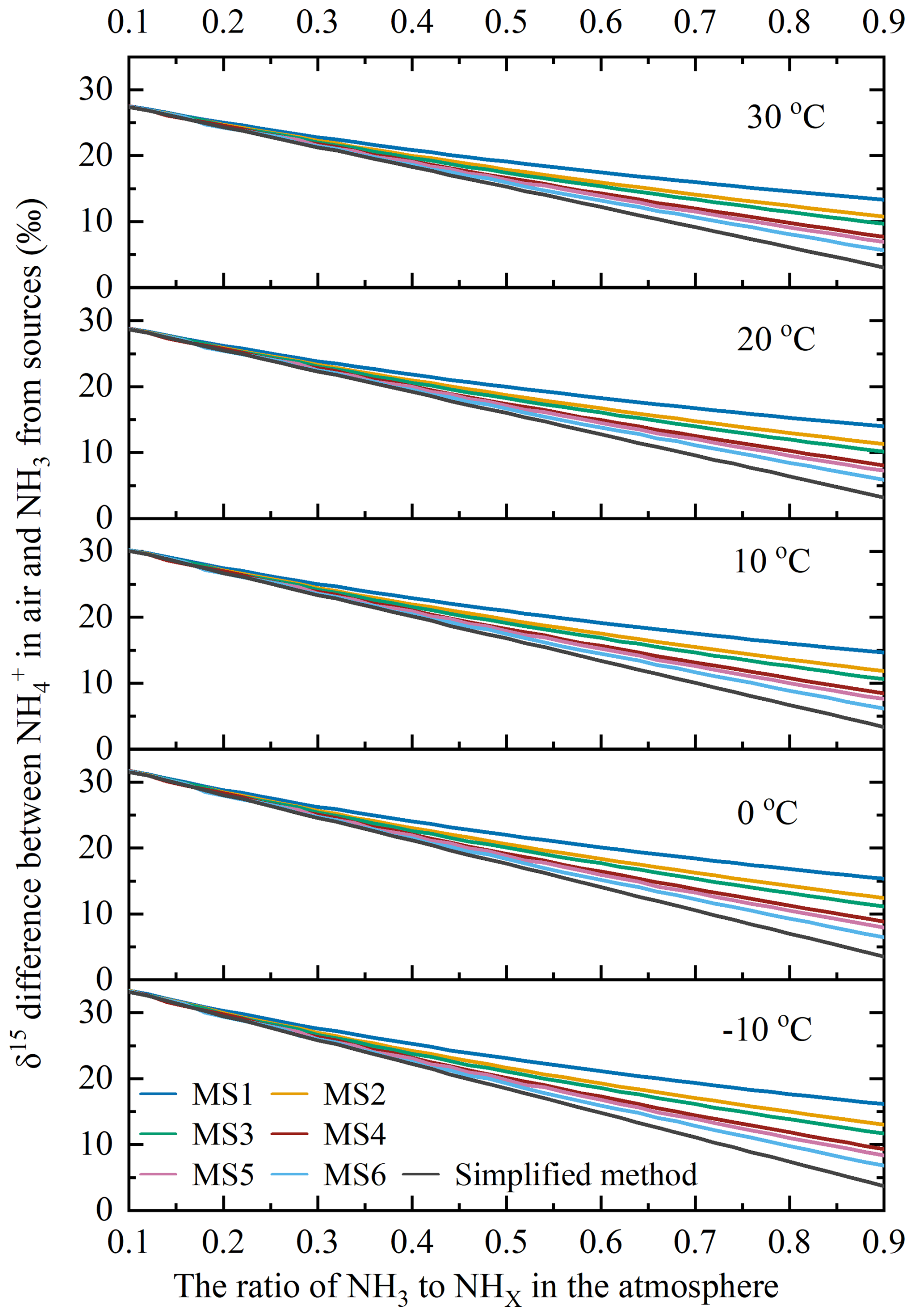
Figure 1 The variation in δ¹⁵N_4a-3s with f at −10, 0, 10, 20, and 30 °C simulated by the six model scenarios and the simplified method. (note: δ¹⁵N_4a-3s is the difference between δ¹⁵N-NH${}_{\mathrm{4}}^{+}$ in the atmosphere and δ¹⁵N-NH₃ emitted from sources, MS1–MS6 are the six model scenarios as listed in Table 1, the simplified method is showed in Eq. 4).

3.2 Sensitivity of δ¹⁵N_4a-3s to Input Parameters

The sensitivity coefficients of each input parameters (D₃, D₄, G₄, and T) to the δ¹⁵N_4a-3s values at 20 °C were calculated by using Eq. (11) across the six model scenarios (see Fig. 2). The sensitivity coefficient of D₃ variation on the simulation results ranged between 2.55 × 10⁻⁵ and 9.32 × 10⁻². The sensitivity coefficient of D₄ and G₄ variations on the δ¹⁵N_4a-3s ranged respectively from 1.77 × 10⁻⁵ to 0.474 and from 3.62 × 10⁻⁴ to 0.494, showing a similar variation signature, which intensified as the value of f increases. Additionally, the range of variation in D₄'s sensitivity coefficient also widened as the value of f increased. However, G₄ did not exhibit this characteristic. The variation range of the sensitivity coefficient of temperature (T) variation on the simulation results was narrow, falling between 0.092 and 0.094, and this influence diminished as the value of f increased. Generally, the sensitivity coefficient exceeding 0.5 is considered that the corresponding input parameter has a sensitive influence on the output result (Cao et al., 2007). It suggested that the influence of each individual input parameter on the simulation output result (δ¹⁵N_4a-3s) did not show obvious sensitivity in the six model scenarios.

In fact, the degree to which input parameters affect the simulation results is not only related to the sensitivity coefficient evaluated based on a single input parameter, but also to the synergistic effect of changes in all input parameters (Wang et al., 2023). In this model simulation, the changes in the δ¹⁵N_4a-3s and f were the results of the input parameter changes. Taking f as a comprehensive input parameter of D₃, D₄, G₄, and T, the sensitivity of f to output results based on the six simulation scenarios was calculated by formula (11). The variation range of the calculated corresponding sensitivity coefficient with f is also shown in Fig. 2. The variation characteristic of this sensitivity coefficient is similar to that of the input parameter D₄, showing that the variation range becomes larger and larger with the increase of f. When the f value was greater than 0.32, the maximum of the sensitivity coefficients obtained by the six simulation scenarios began to be greater than 0.5, that is, the changes in the input parameters (f) were generally considered to have sensitive effects on the output results (δ¹⁵N_4a-3s) (Cao et al., 2007). The maximum range of variation of this sensitivity coefficient was from 0.831 to 3.90 when the f value reached 0.9.

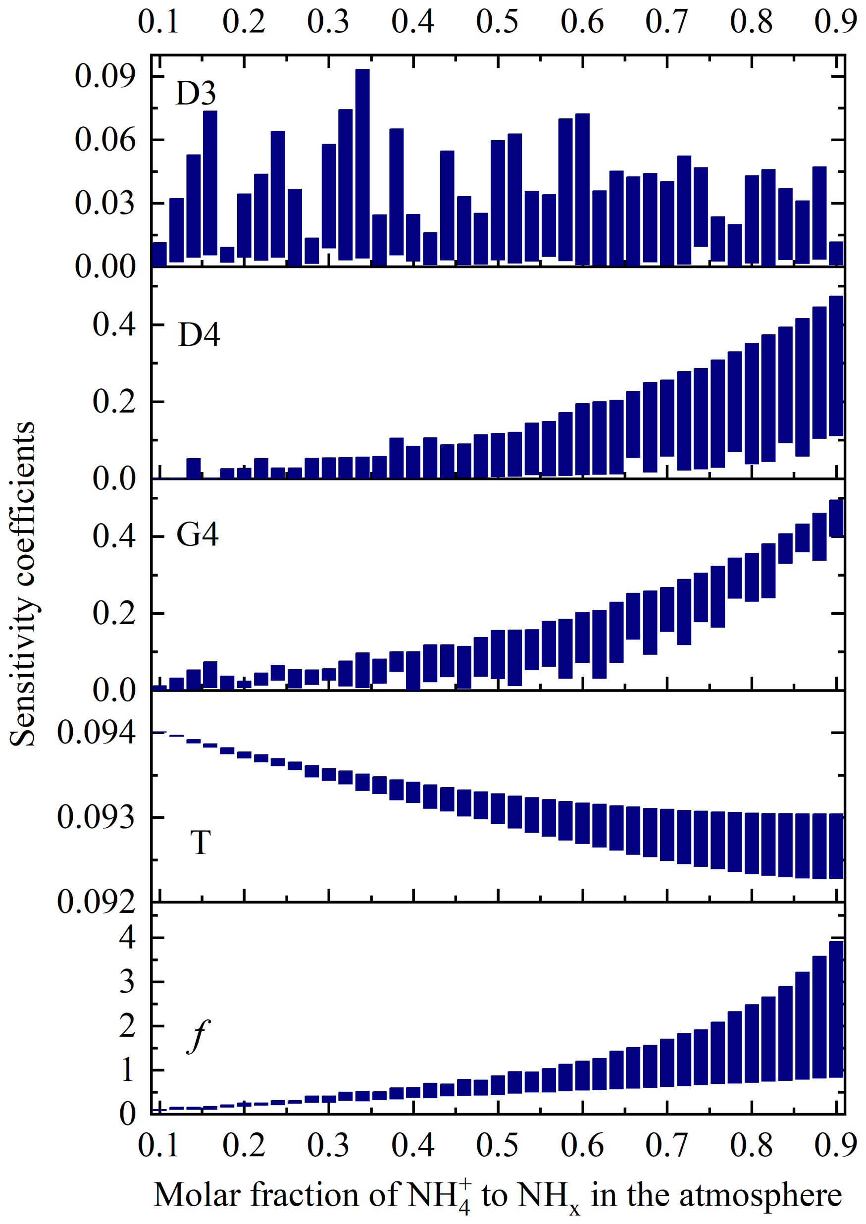
Figure 2 The variation range of sensitivity coefficients of input parameters to the δ¹⁵N_4a-3s values at 20 °C obtained from six simulation scenarios.

These ranges of sensitivity coefficients were generated by six simulation scenarios. To better understand them, the sensitivity coefficients of f to output results (δ¹⁵N_4a-3s) derived from the six simulation scenarios are shown in Fig. S1 of the Supplement. The simulation results of MS1 scenario had the lowest sensitivity to f, while the simulation results of MS6 scenario had the highest sensitivity to f, indicating that large D₄ and G₄ had a greater impact on the simulation results. The finding also indicated that in some urban areas with more acidic gases, especially in mountainous areas, more attention should be paid to the influence of f changes on the source apportionment of NH${}_{\mathrm{4}}^{+}$ in the atmosphere.

3.3 Construction of the Prediction Function for δ¹⁵N_4a-3s

As mentioned earlier, δ¹⁵N_4a-3s is generally calculated using Eq. (3) when apportioning sources of NH${}_{\mathrm{4}}^{+}$ in the atmosphere. The independent variable of this equation included the key influencing parameter f. Based on the form of Eq. (3) and the calculation results of the δ¹⁵N_4a-3s values, we constructed a calculation function for the δ¹⁵N_4a-3s values through nonlinear regression. The form of this nonlinear function is shown in Eq. (12). The coefficient values of B, C, and D in the equation were iteratively fitted for six simulation scenarios. During the fitting process, each simulation scenario took into account different temperature conditions, including −10, 0, 10, 20, and 30 °C.

$$\begin{array}{}\text{(12)}& {\mathit{\delta }}^{\mathrm{15}}{N}_{\text{4a-3s}}=\mathrm{1000}\left({\mathit{\alpha }}^B-\mathrm{1}\right)\left(\mathrm{1}-f^C\right)+D,\end{array}$$

Table 2 lists the iterative fitting values of the coefficients B, C, and D in Eq. (12) for the six model scenarios (MS1–MS6), as well as the determination coefficient (r²) and sum of squares error (SSE), which were often used to evaluate the fitting effect (Sun et al., 2023; Xu, 2017). Figures S2 and S3 of the Supplement show the comparison plots and scatter plots of the δ¹⁵N_4a-3s values calculated by the six fitted equations against the six model scenarios (MS) simulated by the developed model. The coefficients B and C are both greater than 0 and less than 1, and the two coefficients gradually increase from MS1 to MS6, indicating that the Eq. (12) for model scenarios from MS1 to MS6 approaches from nonlinear to linear. The determination coefficients obtained from the regression of the six fitting equations with the simulation results range from 0.967 to 0.998, indicating that these equations can fit the calculated δ¹⁵N_4a-3s values quite well (see Fig. S3 of the Supplement). As shown in Fig. S2 of the Supplement, the maximum deviation between the δ¹⁵N_4a-3s values obtained from the fitting equation and those calculated by the model occurs in the model scenario of MS1. Under −10 °C condition, the deviation reached its maximum value (1.82 ‰) when the f value was 0.9. This largest deviation was also significantly smaller than the variation range of δ¹⁵N values of NH₃, which emitted from various types of sources used in the source apportionment of atmospheric NH${}_{\mathrm{4}}^{+}$ (Gu et al., 2022; Zhang et al., 2023; Feng et al., 2022; Li et al., 2023). This indicated that these fitting equations would not significantly increase the uncertainty of the source-resolved assessment of NH${}_{\mathrm{4}}^{+}$ in the atmosphere when they were used.

3.4 Comparison of Source Apportionment of Atmospheric NH${}_{\mathrm{4}}^{+}$ in Two Case Studies

In order to evaluate the fitting equations as mentioned above using monitoring data, we conducted a source apportionment simulation of NH${}_{\mathrm{4}}^{+}$ again using the atmospheric δ¹⁵N-NH${}_{\mathrm{4}}^{+}$ in the Yellow River Delta in the summers of 2013 and 2021. Apart from the difference in the method of calculating δ¹⁵N_4a-3s values, the model, input data, etc. were consistent with those reported in our previous study (Zong et al., 2023). Briefly, the Bayesian mixing model (MixSIAR) developed by the R language was used for the source apportionment of NH${}_{\mathrm{4}}^{+}$. Four main types of NH₃ emission sources, including fertilizer use (−25.21 ± 9.43 ‰), livestock waste (−16.14 ± 7.98 ‰), vehicle exhaust (+6.62 ± 1.89 ‰), and NH₃ slip (−7.12 ± 7.62 ‰) (Table S3), were considered in the model. In the previous study, we used Eq. (3) (termed as simplified method) to calculate the δ¹⁵N_4a-3s values. In this simulation, we used the MS1 fitting equation to calculate the δ¹⁵N_4a-3s values. This is because these atmospheric particulate matter samples were collected at the Yellow River Delta Ecological Research Station of Coastal Wetland, Chinese Academy of Sciences (37°45^′ N, 118°59^′ E). The Yellow River Delta is an alluvial plain formed by the Yellow River, featuring a very flat terrain (Li et al., 2022; Zhang et al., 2025). Additionally, there are no obvious emission sources from industrial, transportation, and agricultural activities around the sampling site. Many studies regarded this sampling site as an atmospheric background point in North China (Zong et al., 2015; Sui et al., 2015), which met the characteristics of low pollution and a flat terrain in the MS1 scenario. Moreover, the deviation between the δ¹⁵N_4a-3s values calculated by the MS1 method and the simplified method is the largest as shown in Fig. 1, which is more conducive to our evaluation of the degree of difference between the source apportionment results obtained by the two methods.

Table 2 The regression coefficients calculated with δ¹⁵N_4a-3s as the dependent variable and the isotopic fractionation factor (α) and the molar fraction of NH${}_{\mathrm{4}}^{+}$ to NH_x in the atmosphere (f) as independent variables.

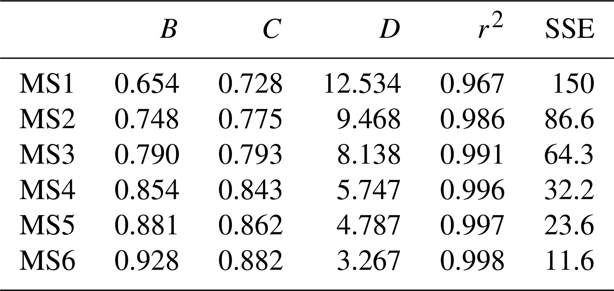
Note: r² is the determination coefficient and SSE is sum of squares error.

For ease of comparing the differences, we summarized both the reported previously results and the findings of this study in Fig. 3. For the sources of atmospheric NH${}_{\mathrm{4}}^{+}$ in 2013, the most noticeable difference between the two source apportionment methods was the significant increase in the contribution proportion of fertilizer application (from 32.9 % using the simplified method to 68.8 % using the fitting equation method) and the corresponding NH${}_{\mathrm{4}}^{+}$ concentration (from 1.33 µg m⁻³ using the simplified method to 2.78 µg m⁻³ using the fitting method). The contributions of the other three emission sources decreased to varying degrees. When we previously used the simplified method for NH${}_{\mathrm{4}}^{+}$ source apportionment, we found that literature reports indicated similar annual NH₃ emissions from fertilizer application and livestock farming in North China, and even in Shandong Province (Zhang et al., 2010). Based on this evidence, we determined that agricultural sources were the main contributors to atmospheric NH${}_{\mathrm{4}}^{+}$ in the Yellow River Delta region in 2013, accounting for 67.4 % (Zong et al., 2023). Recent NH₃ emission inventory results for Shandong showed that farmland fertilizer application sources were closer to the Yellow River Delta than livestock farming sources (Zhu et al., 2024), and that farmland emissions in summer are significantly higher than those from livestock farming (Li et al., 2021). This was consistent with the higher contribution proportion of fertilizer application to atmospheric NH${}_{\mathrm{4}}^{+}$ concentration obtained using the fitting equation method in this study, with the proportion also increasing correspondingly to 82.3 %. Thus, it could be seen that when considering the impact of atmospheric deposition on δ¹⁵N-NH_x in the atmosphere, the contribution of agricultural sources would increase to some extent, and correspondingly, the contribution of non-agricultural sources would decrease.

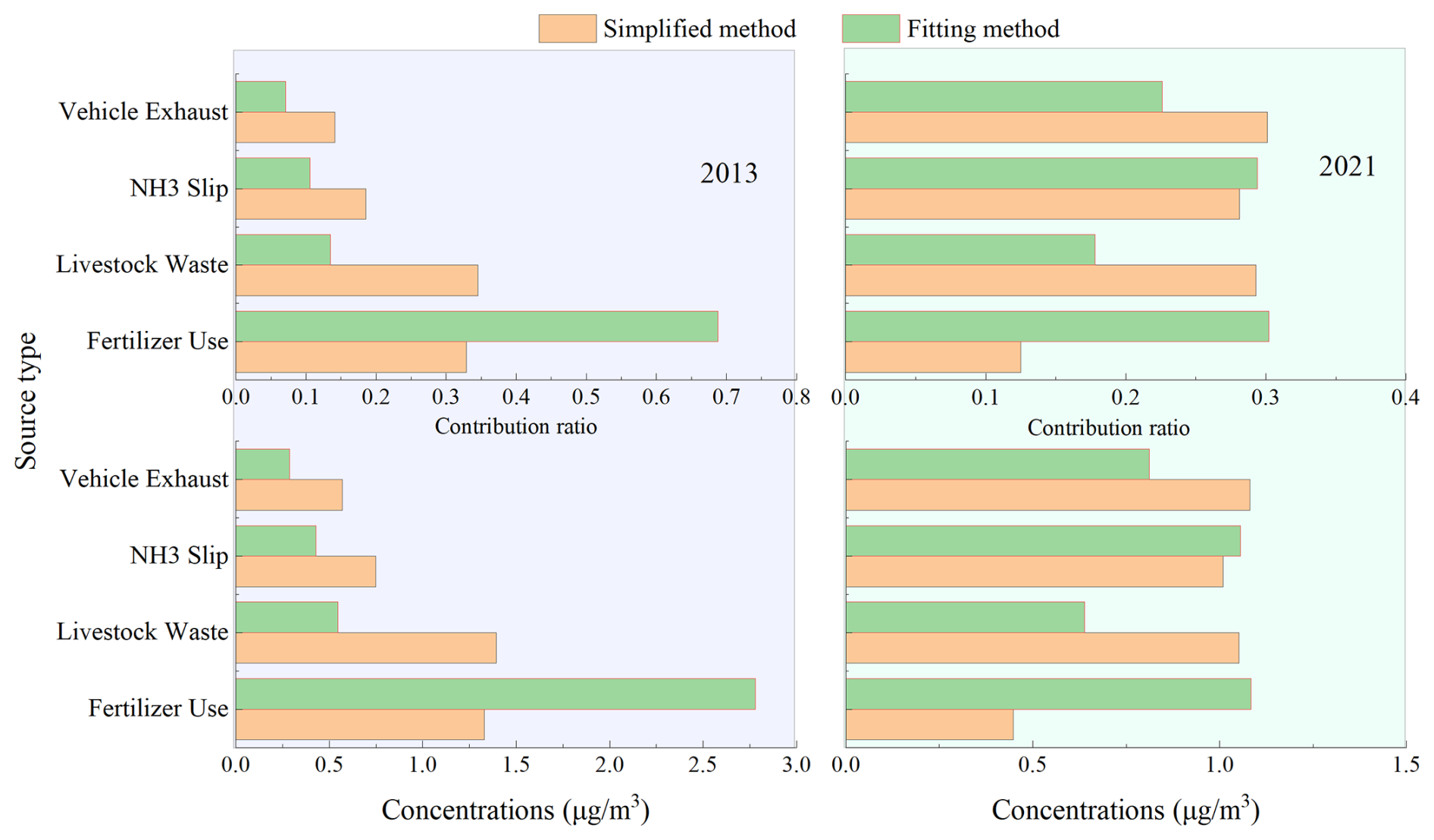
Figure 3 Comparison of the source contribution ratios (top) and source contribution concentrations (bottom) of NH${}_{\mathrm{4}}^{+}$ in the atmosphere of the Yellow River Delta in summer of 2013 (left) and 2021 (right) from four types of NH₃ emission sources using simplified method and the fitting equation method in this study.

For the sources of NH${}_{\mathrm{4}}^{+}$ in the atmosphere in 2021, the most noticeable difference between the two source apportionment methods remained that the contribution proportion of fertilizer application obtained using the fitting equation method was significantly higher (30.2 % by the fitting method vs. 12.5 % by the simplified method) and also significantly higher for the NH${}_{\mathrm{4}}^{+}$ concentration in the atmosphere (1.08 µg m⁻³ by the fitting method vs. 0.45 µg m⁻³ by the simplified method). At the same time, the predicted contribution percentage and concentration of NH₃ emissions from livestock farming by the fitting method was much lower than those by the simple method, 17.8 % and 0.64 µg m⁻³ for the former and 29.3 % and 1.05 µg m⁻³ for the latter, respectively. Thus, due to the offsetting increase and decrease in the contributions of these two types of agricultural sources to atmospheric NH${}_{\mathrm{4}}^{+}$ concentration, the differences in the contributions of agricultural and non-agricultural sources obtained using the two methods were not significant (agricultural sources: 41.8 % using the simplified method vs. 48.0 % using the fitting method; non-agricultural sources: 58.2 % using the simplified method vs. 52.0 % using the fitting method).

To evaluate the applicability of the proposed method in a typical urban environment, observational data of nitrogen isotopes in particulate ammonium (NH${}_{\mathrm{4}}^{+}$) in PM_2.5 collected in Changsha from December 2019 to October 2020 were incorporated in this study (Li et al., 2024). A Bayesian isotope mixing model was applied to quantify the contributions of ammonia sources. Except for the calculation of δ¹⁵N_4a-3s, the model structure, isotopic signatures of the four emission source categories (Table S4), and other relevant parameters were consistent with those reported by Li et al. (2024). Aerosol samples were collected on the rooftop of a building at Central South University of Forestry and Technology (28.1° N, 113.0° E) in Changsha. The sampling site is located in a typical urban functional area, surrounded by high-density residential zones and major traffic roads, and is therefore representative of the urban atmospheric environment of Changsha.

Changsha is located in central China and is characterized by relatively flat terrain within the Xiangjiang River alluvial plain (Zhang et al., 2024; He et al., 2024). The region is subject to strong anthropogenic influences, including vehicular emissions, residential activities, and surrounding agricultural sources, leading to relatively high levels of acidic gases in the atmosphere (Zhai et al., 2014; Ma et al., 2019). According to the classification framework proposed in this study, Changsha is best categorized as the MS5 scenario, representing urban areas with relatively flat terrain and high acidic gas levels. Therefore, the fitted equation developed under the MS5 scenario was applied to calculate δ¹⁵N_4a-3s in this simulation, in order to assess its applicability in a typical urban environment.

The simulation results indicate (Fig. 4) that, compared with the traditional “simplified method”, the use of the fitting equation developed in this study reveals that non-fossil fuel-related emissions dominate in the Changsha region, with their contribution increasing from 55.5 % (agricultural emissions: 28.3 ± 13.4 %, biomass combustion: 27.2 ± 14.3 %) to 59.2 % (agricultural emissions: 30.8 ± 21.1 %, biomass combustion: 28.4 ± 22.3 %). Meanwhile, the contribution from fossil fuel-related sources decreased significantly, falling from 44.5 % (coal combustion: 25.5 ± 14.1 %, vehicle emissions: 19.0 ± 10.5 %) to 40.8 % (coal combustion: 32.7 ± 24.5 %, vehicle emissions: 8.1 ± 8.1 %). It is worth noting that the optimised source contribution structure is closer to the NH${}_{\mathrm{4}}^{+}$ emission inventory for Changsha (Li et al., 2025).

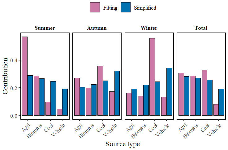
Figure 4 Comparison of source contributions ratios in Changsha from four types of NH₃ emission sources using the simplified approach and the fitted equation method developed in this study.

From a seasonal perspective, both methods indicated pronounced seasonal variations in atmospheric NH${}_{\mathrm{4}}^{+}$ sources in Changsha, generally characterized by an overwhelming dominance of non-fossil sources in summer and a substantial increase in fossil-fuel-related contributions in autumn and winter. In summer, agricultural emissions remained the largest source throughout. After applying the fitted equation, the contribution of agricultural emissions increased from 29.0 % to 57.0 %, whereas that of biomass burning decreased from 26.8 % to 28.5 %. The contributions from coal combustion and vehicle emissions decreased to only 9.7 % and 4.8 %, respectively, and the total contribution of non-fossil sources further increased from 55.8 % to 85.5 %. The optimized source apportionment was more consistent with emission inventory studies conducted in the Changsha–Zhuzhou–Xiangtan region and across China, which have shown that agricultural NH₃ emissions peak in summer and constitute the dominant component of regional NH₃ emissions during this season (Xu et al., 2020; Zhao et al., 2023).

Beginning in autumn, fossil-fuel-related sources gradually became dominant, and the total contributions estimated by the two methods were relatively close (simplified approach: 57.2 %; fitted-equation method: 53.1 %). This result is also more consistent with local observations in Changsha. Xiao et al. (2020) reported that atmospheric NH${}_{\mathrm{4}}^{+}$ in Changsha already exhibited a clear combustion-source dominance in autumn 2017, with fossil-fuel-related sources contributing 51.8 ± 14.9 %.

Winter exhibited the strongest fossil-fuel signature, although the two methods showed marked differences in the inferred structure within fossil-related sources. The fitted equation method identified coal combustion as the overwhelmingly dominant source in winter, with a contribution of 55.9 %, substantially higher than the 24.4 % estimated by the simplified approach. At the same time, the contribution of vehicle emissions was sharply reduced from 34.4 % to 13.5 %. According to the fitted equation method, the contributions of non-fossil and fossil sources in winter were 30.6 % and 69.4 %, respectively, compared with 41.2 % and 58.8 % derived from the simplified approach, further highlighting the dominant role of fossil-fuel emissions in winter. This interpretation is consistent with previous studies. Xu et al. (2020) and Pan et al. (2016) pointed out that winter heating increases coal consumption, leading to substantial increases in NH${}_{\mathrm{4}}^{+}$ and NO${}_{\mathrm{3}}^{-}$ concentrations, and that during severe winter haze episodes, the NH₃ precursor of urban NH${}_{\mathrm{4}}^{+}$ is mainly controlled by fossil-fuel emissions and related industrial processes, while the influence of agricultural sources is weakened.

In the MS1 case, the difference in source contributions in 2013 was significantly greater than that in 2021, which was mainly related to the change in the atmospheric f value (Zong et al., 2023). Specifically, the f value decreased from 71.9 % in 2013 to 41.6 % in 2021. As shown in Fig. 1, with decreasing f values, the discrepancy between the simplified approach and the fitted-equation method gradually became smaller, thereby reducing the difference in source apportionment results obtained by the two methods. In contrast, the f value (Li et al., 2024) in MS5 was 74.6 %, which was close to that of MS1 in 2013. Combined with Fig. 1, this suggests that the variation in the difference between the two methods was closely related to G₄ and D₄: when G₄ and D₄ were at relatively low levels, the difference between the two methods was comparatively small; however, in regions with higher NH${}_{\mathrm{4}}^{+}$ formation ratios (such as MS5 and MS6), the discrepancy between the two methods became more pronounced.

Overall, the use of experimentally validated model parameters (G₄, D₃, and D₄) can further refine the simulation results of source apportionment. Two independent cases, namely the background site MS1 and the urban site MS5, consistently demonstrated that, after accounting for atmospheric deposition, the fitted-equation method can more reasonably constrain the δ¹⁵N_4a-3s value, thereby yielding NH${}_{\mathrm{4}}^{+}$ source apportionment results that are more consistent with actual regional emission characteristics. This indicates that the established fitted equation has good applicability under different environmental gradients and can significantly improve the reliability of NH${}_{\mathrm{4}}^{+}$ isotope-based source apportionment, thus providing a more robust tool for identifying regional ammonia emission sources and formulating emission reduction strategies.

4 Implications and Outlook

Using Bayesian mixing models to apportion sources of atmospheric NH${}_{\mathrm{4}}^{+}$ based on δ¹⁵N data has garnered widespread attention and become a commonly applied tracing method in recent years. As the importance of this tracking method increases, this methodology is also continuously developing and improving. For instance, δ¹⁵N-NH₃ emitted from various sources were continuously reported and supplemented (Chang et al., 2016; Ti et al., 2021; Li et al., 2023), corrections were made for the impact of active and passive sampling on the δ¹⁵N values of atmospheric NH₃ and NH${}_{\mathrm{4}}^{+}$ (Kawashima et al., 2021; Pan et al., 2020), quantitative assessments were conducted on equilibrium and kinetic isotopic fractionation during the gas-to-particle conversion of NH₃ to NH${}_{\mathrm{4}}^{+}$ in the atmosphere, and etc (Walters et al., 2019; Gu et al., 2025).

NH₃ emitted into the atmosphere undergoes continuous gas-to-particle conversion between NH₃ to NH${}_{\mathrm{4}}^{+}$ as it is transported and dispersed, ultimately leaving the atmospheric system primarily in the form of NH₃ to NH${}_{\mathrm{4}}^{+}$ through deposition. The gas-to-particle conversion process of NH₃ to NH${}_{\mathrm{4}}^{+}$ in the atmosphere exhibits significant isotopic fractionation, and there are marked differences in the deposition ratios of NH₃ to NH${}_{\mathrm{4}}^{+}$, leading to continuous changes in the atmospheric δ¹⁵N-NH_x values. This change is widely recognized but has not been fully considered in the source apportionment method based on nitrogen isotope. This study developed a model to quantitatively assess the variation pattern of atmospheric δ¹⁵N values under atmospheric deposition scenarios. Furthermore, a regression equation was constructed through nonlinear fitting to facilitate the application of this research finding in the tracing of atmospheric NH${}_{\mathrm{4}}^{+}$. Two comparative case studies revealed that using simplified methods for source apportionment of NH${}_{\mathrm{4}}^{+}$ could overestimate the contribution of non-agricultural sources. This understanding could partly explain the discrepancies in atmospheric ammonium sources derived from emission inventory methods and nitrogen isotope methods (Chen et al., 2022; Gu et al., 2025; Chang et al., 2019a).

The key parameters in this model (e.g., D₃, D₄, and G₄) are currently set based on a synthesis of literature values. These parameters exhibit significant spatial heterogeneity and temporal dynamics, influenced by factors such as land surface type, meteorological conditions, and atmospheric chemical composition. Future work requires multi-site, multi-season synchronous observations combining micrometeorological methods and isotopic measurements to directly obtain parameter values under different environments. This will enhance the model's empirical foundation and regional applicability.