Characterisation of cloud shadow transition signatures using a dense pyranometer network

The small-scale variability of solar radiation including 3D radiative effects is poorly observed and understood. In this study, we characterise the transition of global solar horizontal irradiance from sunshine to cloud shadow and attribute the transition signature to 3D radiative effects. This analysis is based on 5 case days with shallow cumulus clouds at the ARM Southern Great Plains Central Observatory. Observations are conducted by PyrNet, a network of 60 autonomous pyranometer stations deployed during a field campaign in summer 2023. Complementary observations of cloud mask and shadow motion are derived from the Clouds Optically Gridded by Stereo (COGS) product. Concentrating on shallow cumulus clouds, we explore how geometrical effects and the macro- and microphysical properties of clouds affect the pattern of solar irradiance variation close to the cloud shadow edge. Individual cloud entities and cloud motion vectors are identified using COGS. We discovered that the amplitude of radiation enhancement can reach 20 % above the clear sky values. Significant influence factors are the size of the cloud gaps, the height of the cloud base and the geometry between the sun and the clouds. The distance from the cloud at which radiation enhancement remains significant depends on the effective radius of the cloud droplets, cloud optical depth, and solar zenith angle. Our findings underscore the necessity of accounting for these 3D effects in atmospheric modelling to enhance the representation of solar radiation processes and are a step towards the development of transition signature parametrisations for photovoltaic energy applications.

1 Introduction

Solar radiation in general, and global horizontal irradiance (GHI) in particular, exhibits strong spatio-temporal variability during broken cloud conditions, such as shallow cumulus clouds (e.g., Schroedter-Homscheidt et al., 2018; Gristey et al., 2020). This variability is of scientific interest because it impacts the coupled atmosphere-land system, including the energy balance and the water cycle (Vilà‐Guerau De Arellano et al., 2023). It affects plant photosynthesis (Durand et al., 2021; Darko et al., 2023), as well as the feedback mechanisms that govern cloud formation and organisation (Jakub and Mayer, 2017). These processes are sensitive not only to the total amount of incoming solar energy, but also to its spatial and temporal distribution, which is also of particular interest from an engineering standpoint for the performance and stability of photovoltaic (PV) power generation (e.g., Barry et al., 2020; Kreuwel et al., 2021; Omoyele et al., 2024). The scales of this variability range from seconds and metres to hours and kilometres (e.g., Madhavan et al., 2017; Schroedter-Homscheidt et al., 2020; Mol et al., 2024). Accurately capturing this variability is crucial, but it remains a significant challenge for current atmospheric models and satellite observations, even for those with enhanced spatial and temporal resolution (e.g., Hourdin et al., 2017; Schreck et al., 2020; Verbois et al., 2023).

A significant challenge in accurate estimation of GHI through both observational data and modelling arises in broken cloud conditions. Here, 3D radiative effects, such as local irradiance enhancement due to clouds (cloud enhancement, CE) and shadow displacement, become increasingly relevant (e.g., Gueymard, 2017). Since clouds and radiation are physically coupled in the atmosphere, inaccuracies in simulating one component can lead to cascading errors in the other. Although many studies have investigated these effects using 3D radiative transfer schemes with synthetic or modelled cloud fields (e.g., Hogan et al., 2019; Meyer et al., 2022) as input, observational validation is rare, particularly at finer spatio-temporal scales (e.g. sub-kilometre and seconds) (Villefranque and Hogan, 2021).

While the Baseline Surface Radiation Network (BSRN) and similar programmes provide high-quality long-term irradiance records, their data are typically limited to single-point measurements with one-minute temporal resolution (Driemel et al., 2018). This level of detail is insufficient for capturing sub-kilometre-scale irradiance patterns and their rapid fluctuations. Studies, such as those of Tomson (2010) and Yordanov et al. (2013), have stressed the need for at least 1 Hz sampling to resolve high variability and CE during cloud-shadow transitions. Mol et al. (2023) also emphasised the lack of spatially dense GHI data sets at resolutions that match cloud-induced variability scales.

Dense pyranometer networks have shown potential to fill this gap. Early efforts were made in 2009 deploying six stations in San Diego (Lave et al., 2012) and in 2010 a setup of 17 sensors to analyse spatial irradiance variability in Hawaii (Sengupta and Andreas, 2010; Tabar et al., 2014). Using observations obtained with the pyranometer network (PyrNet) of the Leibniz Institute for Tropospheric Research (TROPOS) during the HOPE (High Definition Clouds and Precipitation for advancing Climate Prediction (HD(CP)2) Observational Prototype Experiment) field campaign in 2013 (Macke et al., 2017), Madhavan et al. (2016, 2017) demonstrated strong spatial decorrelation of GHI under broken clouds, with irradiance fluctuations becoming uncorrelated beyond about 1 km at high temporal resolution. Lohmann et al. (2016) and Ranalli et al. (2020) used the same data to model smoothing effects in distributed photovoltaic systems and to show how irradiance variability propagates into power generation. He et al. (2024) also utilised this data to identify bimodal irradiance patterns due to cloud shadows and CE, and recommended optimising sensor layouts to improve observational efficiency. More recently, Mol et al. (2024) advanced the field by deploying a network of spectral sensors during the FESSTVaL (Field Experiment on submesoscale spatio-temporal variability in Lindenberg) and LIAISE (Land surface Interactions with the Atmosphere over the Iberian Semi-arid Environment) campaigns in 2021, documenting characteristic patterns of broadband and spectral GHI under various cloud types, including shallow cumulus. Tijhuis et al. (2023) derived parametrisations of diffuse radiation under shallow cumulus using these measurements.

Other relevant studies focus on specific radiative signatures or modelling tools. Berg and Kassianov (2008) produced a 5-year climatology of fair-weather cumulus at the Atmospheric Radiation Measurement facility in the Southern Great Plains (ARM-SGP), showing how their structure affects cloud fraction and radiative transfer. Deneke et al. (2021) and Wiltink et al. (2024) validated a downscaling method for Meteosat-derived GHI, highlighting cloud-type-dependent biases and the importance of ground truth at high resolution. Mol and Van Heerwaarden (2025) published a comprehensive overview of the mechanism of the 3D radiative effect in the vicinity of clouds using their radiative transfer model, building on the work of Tijhuis et al. (2023) and Mol et al. (2024). While our study shares a methodological overlap with these recent works, it differs in three key ways: (1) the PyrNet layout consists of 60 stations spread over an area of approximately 6 × 8 km which enables us to derive a large set of time series of cloud-shadow transition signatures, thus allowing for stable statistics, (2) we use the COGS (Clouds Optically Gridded by Stereo) 4D cloud mask for scene reconstruction and derive the cloud motion vector instead of relying on Large Eddy Simulation (LES) output, and (3) we leverage co-located measurements from the central ARM-SGP, including cloud microphysical properties, to study important features required for GHI parametrisation. Given the limited availability of high-resolution spatially distributed GHI data, our contribution is perfectly suited to fill this gap.

This study explores several research questions; first, is it possible to acquire direct observational evidence of 3D radiative effects at cloud edges, effects that are usually deduced from simulations? Second, how do the characteristics of cloud-shadow transitions vary based on the sun-cloud geometry and the macro- and microphysical properties of clouds? Finally, what observed characteristics are most relevant for the development of empirical models that aim to accurately represent GHI patterns in shallow cumulus conditions? We address these questions using data from the dense layout of PyrNet in the S2VSR (Small-Scale Variability of Solar Radiation) field campaign (Witthuhn et al., 2024) near the ARM-SGP site, together with auxiliary observations of cloud structure, motion, and optical properties. We focus on 5 d with shallow cumulus conditions.

The paper is structured as follows. Section 2 describes the field campaign and data sets used. In Sect. 3, we define the analytical framework. Section 4 presents the main results, focussing on the patterns of irradiance variability and transition characteristics and relating our findings to previous work. Finally, in Sect. 5, we conclude with a summary and an outlook, including potential future applications of the results within the broader context of PV forecasting and radiative transfer modelling.

2 S2VSR campaign

The S2VSR field campaign was carried out from June to August 2023 at the ARM-SGP observatory in Billings, Oklahoma, USA. PyrNet stations were deployed and arranged in a grid pattern around the observatory (latitude: 36.607° N, longitude: −97.488° E; see Fig. 1). The central motivation of the campaign was to connect cloud properties with GHI fluctuations, to evaluate the representativeness of single-point observations, and compare ground data with high-resolution satellite products, and atmospheric models. To address these goals, this campaign offers a unique opportunity through the combined availability of PyrNet observations (Sect. 2.1), the COGS 4D cloud mask product (Sect. 2.2), and the routine measurements conducted at the observatory (Sect. 2.3).

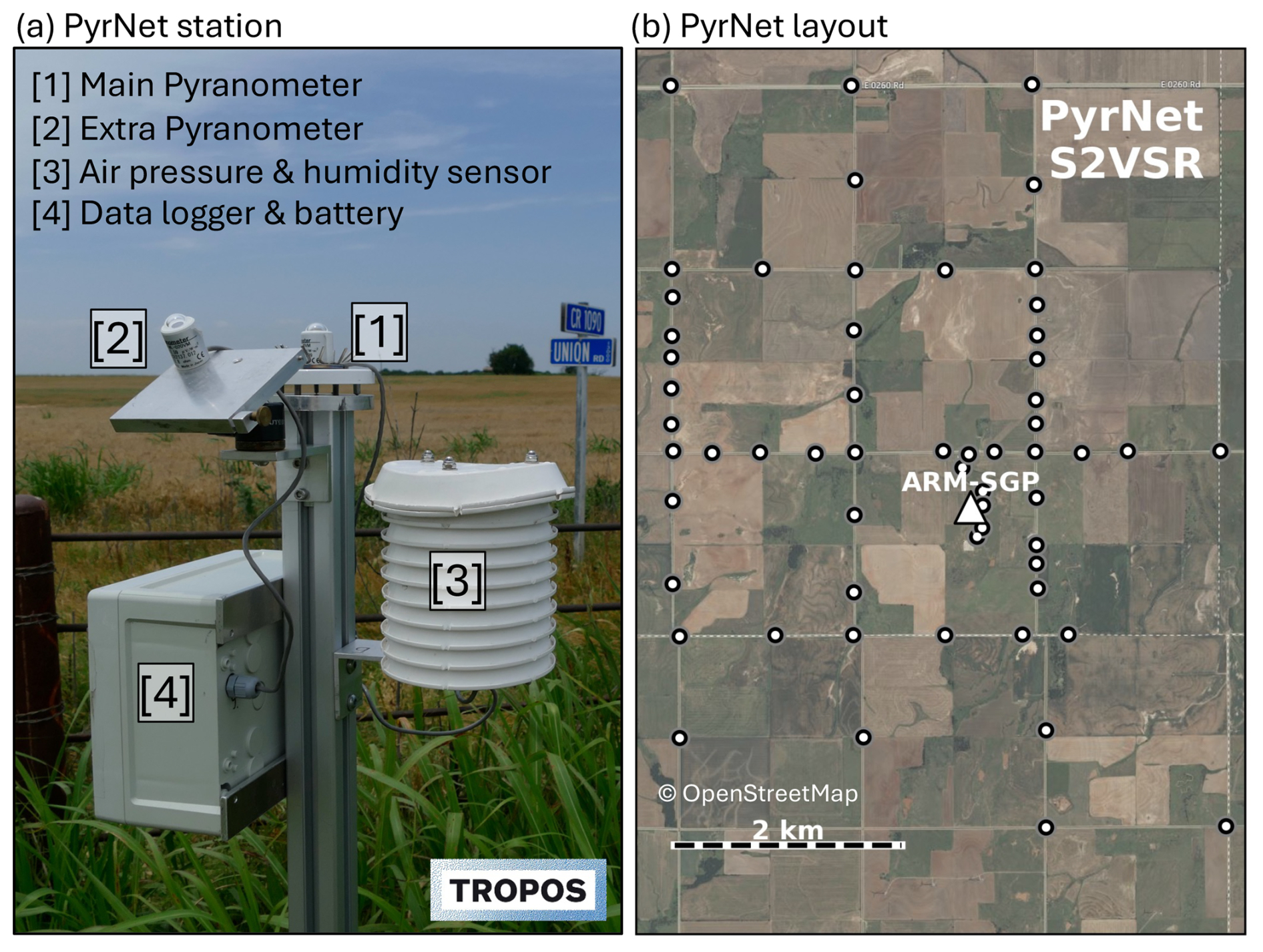
Figure 1 Annotated PyrNet station in panel (a): In this study, we used data exclusively from the main pyranometer [1], which was horizontally aligned for GHI measurement. The extra pyranometer [2] is used for tilted irradiance measurement. In addition, air pressure and humidity were monitored [3]. The data logging device [4] integrates a GPS antenna and records data on an SD card, with a battery that lasts approximately 10 d. S2VSR layout in panel (b): The white dots indicate the placement of every PyrNet station during the S2VSR campaign around the ARM-SGP site (marked by a white triangle). The shade of the ring surrounding the white dots indicates the measured broad transmittance ($\frac{\mathrm{GHI}}{{\mathit{\mu }}_{\mathrm{0}}{I}_{\mathrm{0}}}$, with I₀ the solar beam irradiance at the top of the atmosphere and μ₀ the cosine of the solar zenith angle). The sun's azimuth direction is shown by the dashed yellow line. The map is overlaid with the COGS cloud mask represented in a white transparent hue within the product's valid area (dashed line). The projected cloud shadow, derived from this mask and the sun's position, is depicted in a black transparent hue.

Typical summer weather conditions were experienced during the campaign period, with occasional thunderstorms and heavy rain. Agricultural activities, road dust displacement, and fires sometimes produced high concentrations of aerosols in the atmospheric boundary layer that polluted the sensor domes. Daily cloud conditions during the campaign, as determined using the ARM Cloud Type Classification product (Zhang et al., 2018), showed 25 % cloud-free conditions and 50 % single-layer cloud conditions, of which 45 % were attributable to convective clouds. Single-layer low cumulus clouds appeared in 14 % of all cloudy cases.

In this study, we focus on 5 d during S2VSR with single layer shallow cumulus situations and for which the COGS product was available (13 and 18 June, 7 July, 22 and 27 August 2023). During these days, the weather pattern remains largely similar. Cloud shadow speeds fluctuate between 2 and 6 m s⁻¹, and the clouds are primarily advected from south-easterly to south-westerly directions. In addition, cloud cover ranged from 20 to 80 %.

2.1 PyrNet

The PyrNet is a mobile surface radiation observation network originally developed for the HOPE field campaign (Madhavan et al., 2016; Macke et al., 2017). Its primary purpose is to capture the small-scale spatio-temporal variability of cloud affected short-wave radiation fields at the surface. During the S2VSR campaign, 60 stations were deployed around the ARM-SGP site, along the roads at the borders of fields (see Fig. 1). The covered area spans about 5 × 6 km with PyrNet stations distributed more densely around the ARM-SGP station, with distances of less than 100 m from each other, and further spread out in the outer area, with distances of up to 1.5 km from the next station. Each station is equipped with one or two Eko Instruments ML-020VM pyranometers. At the 30 stations with two pyranometers, solar irradiance from a tilted plane is measured along the GHI measurement (see Fig. 1a), but not used in this study.

The Eko Instruments ML-020VM pyranometers are of photoelectric type which have a spectral range from 400 to 1100 nm and response time (to reach 95 % of final output value following a sudden change in irradiance) of about 10 ms. Due to this response time they are perfect for fast sampling of rapid changes of GHI (Madhavan et al., 2016). During S2VSR, GHI is sampled with 10 Hz resolution, and then aggregated to 1 s by averaging sub-second samples. This processing stage involves quality control to identify data compromised by factors such as severe pollution or misalignment. Pollution of the sensor domes can arise unexpectedly due to activities such as nearby agricultural operations or traffic on the roads. Significant rainfall events can leave the soil muddy and cause the stabilisation rod to shift from its initial position. The automated testing algorithm includes extremal and physical limit tests of GHI data adapted from the BSRN quality check procedure (Schmithüsen et al., 2019). In addition, the recorded GHI of each network station is verified using the rolling 30 min average GHI value. Any station readings that fall outside a tolerance of ±10 % (or ±15 % when the solar elevation < 25°), such as stations affected by shading from nearby structures, are identified as anomalies. Each PyrNet station underwent weekly maintenance, which involved sensor cleaning and realignment. Additionally, manual quality checks were performed and recorded during these maintenance periods.

The absolute standard uncertainty for PyrNet pyranometers is estimated to be up to 10 % per sample, according to (Madhavan et al., 2016). Given that this study primarily examines the rapid temporal variations in the signal, this uncertainty is not of significant concern as long as there is comparability among individual stations. To enhance the comparability of data from different stations, we have implemented cross-calibration and cosine correction techniques. To achieve this, all stations were collectively installed on a deck of the ARM-SGP guest instrument facility one week before the campaign, from 2 to 8 June 2023. Cross-calibration was performed versus the primary standard baseline radiation station (Shi et al., 2003) following ISO 9847 standards, resulting in new absolute calibration factors assigned to each station. To improve comparability, a cosine correction was performed versus the solar zenith angle as in Barry et al. (2023), resulting in the following correction factor:

$$\begin{array}{}\text{(1)}& C\left({\mathit{\mu }}_{\mathrm{0}}\right)=-\mathrm{2.227}{\mathit{\mu }}_{\mathrm{0}}^{\mathrm{3}}+\mathrm{4.366}{\mathit{\mu }}_{\mathrm{0}}^{\mathrm{2}}-\mathrm{2.524}{\mathit{\mu }}_{\mathrm{0}}+\mathrm{1.385}\end{array}$$

where μ₀ denotes the cosine of the solar zenith angle. The calibration and cosine correction procedures are documented in the PyrNet repository documentation (Witthuhn et al., 2023).

2.2 Cloud and shadow masking

To identify the location of shadows and clouds, we used the COGS 4D product (Romps and Öktem, 2018) in our analysis, which provides a gridded shallow cumulus mask by triangulation of cloud features detected by three camera pairs in high resolution. The observation volume is centred on the ARM-SGP central facility and spans a cube of 6 × 6 × 6 km at a spatial resolution of 50 m and a temporal resolution of 20 s.

Contours of cloud objects are generated for each height level containing cloudy voxels, and are translated horizontally to the corresponding shadow locations based on the height of the level and sun geometry. Subsequently, the contour polygons from different height levels are combined using their geometric union, and subsequently converted back into a raster field. For these operations, the Python libraries contourpy and Shapely are used. Special attention is given to preserve the information on valid data given by the COGS product.

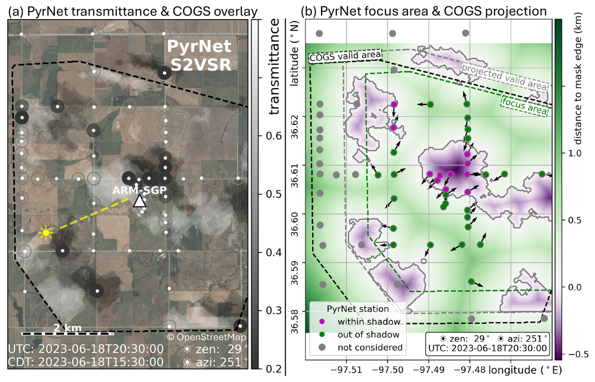
Figure 2 S2VSR layout in panel (a): The white dots indicate the placement of every PyrNet station during the S2VSR campaign around the ARM-SGP site (marked by a white triangle). The shade of the ring surrounding the white dots indicates the measured broad transmittance ($\frac{\mathrm{GHI}}{{\mathit{\mu }}_{\mathrm{0}}{I}_{\mathrm{0}}}$, with I₀ the solar beam irradiance at the top of the atmosphere and μ₀ the cosine of the solar zenith angle). The sun's azimuth direction is shown by the dashed yellow line. The map is overlaid with the COGS cloud mask represented in a white transparent hue within the product's valid area (dashed line). The projected cloud shadow, derived from this mask and the sun's position, is depicted in a black transparent hue. Focus and projected areas in panel (b): Contours of the projected shadow mask derived from the COGS cloud mask and the sun's position are displayed. The colours indicate the distance to the closest cloud shadow edge (negative within a shadow). At each PyrNet station location within the focus area (green/magenta for out-/inside a cloud shadow), an arrow shows the direction to the closest shadow edge. The dashed lines represent the valid area of the COGS cloud mask (black), the projected valid area to the surface derived from the cloud base height and sun's position (grey) and the focus area (green) with border of 0.005° to the projected valid area. PyrNet locations outside of the focus area (grey dots) are not considered for distance and angle calculations.

In Fig. 1b, we visualize the COGS cloud mask alongside the projected cloud shadow mask. These masks were used to compute the Euclidean distance and angle from the respective edges of the cloud or its shadow at distinct time intervals at PyrNet sites, utilizing the SciPy ndimage package (Virtanen et al., 2020). Figure 2 depicts the determined distances and angles to shadow edges in the same situation as shown in Fig. 1. Measures of distances and angles to the nearest mask edge are computed exclusively for stations located within the designated focus area depicted in Fig. 2. This region is derived from the valid area of the COGS product, projected onto the surface by considering the sun's position and average CBH from COGS. Moreover, a boundary of 0.005° is excluded to prevent calculating the distance to the valid area border instead of to a mask edge. For the calculation of distance and angle relative to the cloud mask, the 3D COGS cloud mask is vertically projected onto the surface plane, indicating if a cloud is situated directly above a station or its horizontal distance from it.

The 2D shadow mask projected from COGS is subsequently utilized to derive the flow vector of the present cloud field. We employed the Farnebäck optical flow algorithm as implemented in the OpenCV library (Bradski, 2000; Farnebäck, 2003), computing the flow vector for each frame at a 20 s interval, and we applied a rolling average over a 10 min duration. We analyse the time series data collected by PyrNet relative to the flow to ensure data comparability across different days with varying wind speeds. Throughout the study, the distance relative to the flow is always computed as the product of the flow speed with the time step.

2.3 ARM-SGP routine observations

The SGP atmospheric observatory, operated as a US Department of Energy's ARM user facility, has been collecting continuous, high-quality atmospheric data in north-central Oklahoma since 1992. Covering about 4600 km², ARM-SGP hosts a dense array of in situ and remote sensing instruments at its Central Facility, providing detailed records of temperature, moisture, wind, aerosols, clouds, and radiative energy for research and model evaluation.

In this study, we use several routine ARM-SGP devices and corresponding data products: (1) the Microwave Radiometer (MWR), which measures atmospheric microwave emissions at 23.8 and 31.4 GHz to retrieve liquid water path using site-specific statistical algorithms (Cadeddu and Tuftedal, 1993); (2) the Ceilometer (CEIL), which determines cloud-base heights for up to three layers with ±5 m uncertainty and 16 s resolution (Zhang et al., 1996); (3) the Multi-Filter Rotating Shadowband Radiometer (MFRSR), which provides overcast liquid-cloud optical depth (415 nm) and, paired with MWR data, liquid effective radius at 20 s intervals (Zhang, 1997); (4) the Total Sky Imager (TSI), which captures hemispheric daylight sky images every 15 min and estimates fractional sky cover (Flynn and Morris, 2000); and (5) the Broadband Radiometer Station (BRS), which records 1 Hz GHI using secondary standard pyranometers with quality standards comparable to BSRN (Shi et al., 2003).

3 Methods

In this study, we analyse observations of GHI for shallow cumulus cloud conditions. The values for 13 June 2023 are displayed in Fig. 3. As clear sky reference, we use the simplified Solis clear sky model (Ineichen, 2008) from the pvlib-python implementation (Anderson et al., 2023). This model was evaluated versus reference observations and shows good agreement given the minimal input variables required (Ineichen, 2016; Witthuhn et al., 2021). Radiation enhancement occurs in the gap between two clouds (shadows) due to several scattering mechanisms. Regarding these mechanisms, we stick to the naming conventions proposed by Mol and Van Heerwaarden (2025). Essentially, the side-escape mechanism is dedicated to radiation enhancement due to reflection on cloud edges, forward- and downward-escape describe enhanced radiation below the cloud due to forward-scattering of cloud droplets in optically thin cloud and/or multiple scattering in optically thicker clouds. Lastly, the albedo-enhancement describes diffuse radiation enhancement below the cloud due to multiple reflections from the surface and cloud base. When cloud (shadow) gaps are narrow, GHI observed within those gaps is higher than the reference clear sky value due to the side-escape mechanism. We defined a radiation enhancement level, shown as a black line in Fig. 3, by computing a two hour rolling mean over observed GHI values greater than the clear sky GHI and without a significant slope of 5 W m⁻² s⁻¹, similar to Lappalainen and Valkealahti (2015), to filter out the steep transition into cloud shadow GHI. As outlined in the section below, we analyse shadow transition signatures with respect to clear sky and the enhancement level.

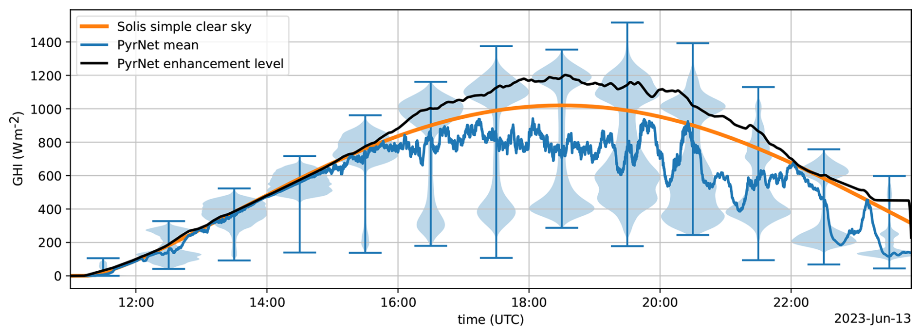
Figure 3 Observed GHI distributions from PyrNet at 13 June 2023 in hourly bins. The distributions as violin plot indicating extrema values in each bin and are of bi-modal shape in the presence of clouds (cloud shadow and shadow gap with enhanced radiation). In addition, the GHI mean over all PyrNet stations in 1 min resolution (blue line) and the calculated enhancement level in cloud shadow gaps (black), and the clear sky reference modelled by the Solis simple model (orange) are shown.

We refer to a cloud shadow transition signature of a GHI time series as follows: GHI values start low in the cloud shadow at the sharp transition from low to high or enhanced values at the cloud shadow edge. This continues until a certain distance in direct sunlight in the cloud shadow gap, where observed GHI values are larger than or equal to the clear sky reference GHI. In the following section, we describe how cloud shadow transition signatures are identified from the PyrNet data and our approach to achieve comparability and meaningfulness with regard to external variables.

3.1 Identification of cloud shadow transition signatures

In order to detect transition signatures in the GHI data from all PyrNet stations, we started by masking all GHI values lower than the clear sky reference. In addition, strong events with a slope of GHI values larger than 5 W m⁻² s⁻¹ are identified as transition to the cloud core shadow (Lappalainen and Valkealahti, 2015). Then the time series before and after a shadow event are analysed. For analysing them in a unified way, the time series before a shadow event is flipped, so that the shadow will always be the start of the snipped time series. Using the SciPy algorithm find_peaks, we identified the enhancement peak close to the shadow edge. Thereafter, employing the flow vector of the cloud field (Sect. 2.2), the time series are converted into distance series along the flow direction, centred on the detected peaks. For each of these peaks, a data segment is extracted that extends 60 m towards the cloud shadow from the peak location and 600 m towards the unshaded side of the enhancement peak. These bounds are chosen somewhat arbitrarily based on manual inspection: the first bound is set such that the GHI values fall below the clear-sky level within the shadowed part of the segment, while the second bound is selected where most segments have already intersected another cloud shadow. As a last step, we filtered out the snipped time series that already encountered another shadow within 300 m from the peak, to ensure a relatively undisturbed signature by nearby cloud mechanisms (except side-escape).

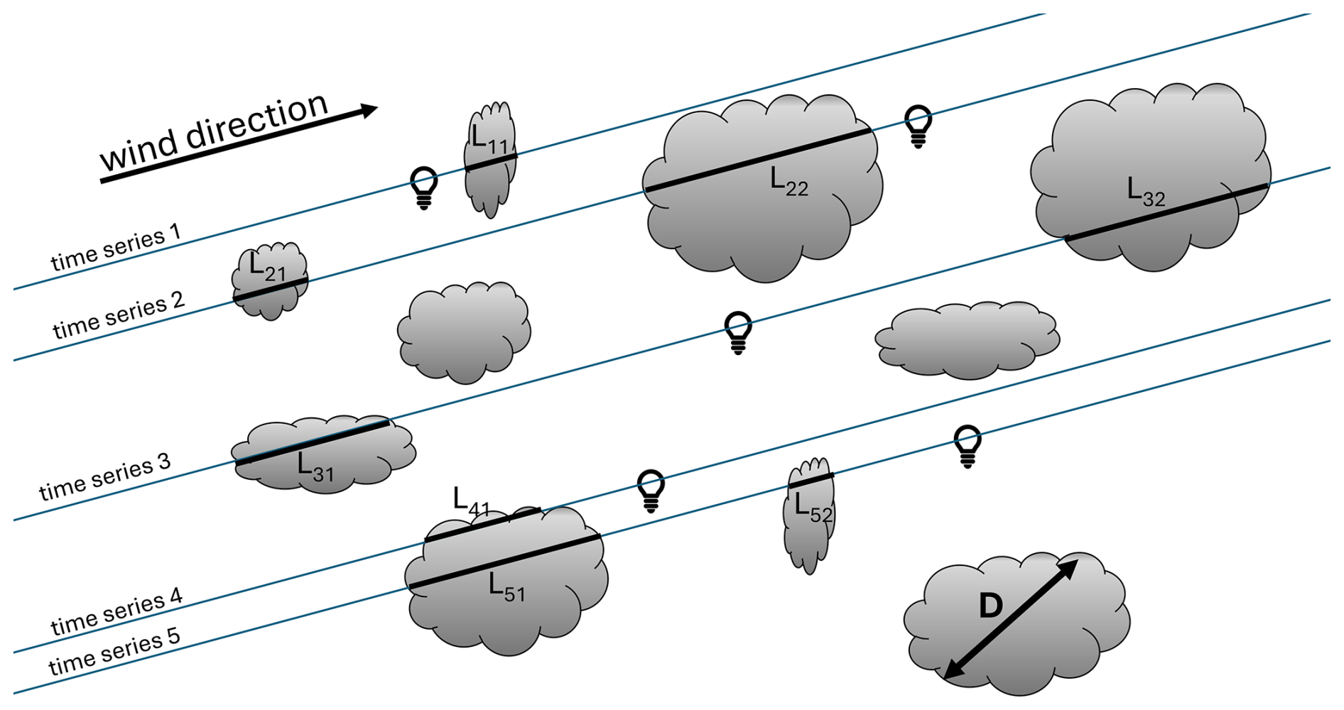
Figure 4 Diagram depicting how cloud shadow and sun light chord lengths are observed with PyrNet. Chord lengths describe the time period of a measured time series in a specific state, in this case staying in the shade or in the shadow gap. Cloud shadow chord lengths L_ij sampled by PyrNet, with i denoting the instrument number (e.g. the number of time series) and j the cloud chord number within one time series. The measure D represents a linear cloud size representation, which differs from the cloud shadow chord length recorded by PyrNet for two key reasons. Firstly, the relationship between shadow size and actual cloud size varies based on sun elevation and cloud height. Secondly, because the measurements are taken at fixed positions, the recorded shadow chord lengths capture only arbitrary cross-sections of the respective cloud shadows passing the stations. This figure is adapted from Romps and Vogelmann (2017).

Amid the intrinsic limitations of 1D time series data, the precise distance to the nearest cloud shadow edge is unknown. Figure 4 illustrates how this limitation contrasts with the 2D information available from COGS data. Since time series function as linear cross-sections through a cloud shadow field, a cloud shadow may be in close proximity but not interrupt the direct sunbeam to the measuring station, meaning that the shadow is not detected in the time series data. For analysing transition signatures from 1D data, our focus is on the enhancement peak region near the shadow edge, as it is likely that radiation enhancement is mostly originating from the cloud, which casts the shadow.

3.2 Fitting of cloud shadow transition signatures

To interpret transition signatures relative to the clear sky reference and to compare them against additional variables, we focus on the magnitude of the enhancement peak T_peak and how far radiation enhancement persists in distance to the cloud shadow. We chose to derive the e-folding distance x_e, which is the distance from the peak location where radiation enhancement falls below $(T_{\mathrm{peak}}-\mathrm{1})/e$, where e is the Euler number, as sketched in Fig. 5. Deriving these measurements from a single observed time series is challenging due to high fluctuation around the peak region, stemming from the strong cloud inhomogeneity. Therefore, we assumed that an undisturbed transition signature can be represented by the following modified Buckingham (exp,6) potential function (Mason, 1954):

$$\begin{array}{}\text{(2)}& \begin{array}{rl}T\left(x\right)=& \mathrm{1}-{\displaystyle \frac{\mathit{ϵ}}{\mathrm{100}(\mathit{\alpha }-\mathrm{6})}}\\ & \cdot \left(\mathrm{6}\cdot \exp \left(\mathit{\alpha }-{\displaystyle \frac{\mathit{\alpha }\cdot x}{\mathrm{10}\mathit{\sigma }}}\right)-\mathit{\alpha }{\left({\displaystyle \frac{\mathrm{10}\mathit{\sigma }}{x}}\right)}^{\mathrm{6}}\right),\end{array}\end{array}$$

where T denotes the GHI normalised to the clear sky reference GHI. The original potential function is modified in the way that ϵ describes the magnitude of the peak of the transition signature in percent versus clear sky by applying an offset of 1.

$$\begin{array}{}\text{(3)}& \mathit{ϵ}=\mathrm{100}\times (T_{\mathrm{peak}}-\mathrm{1})\end{array}$$

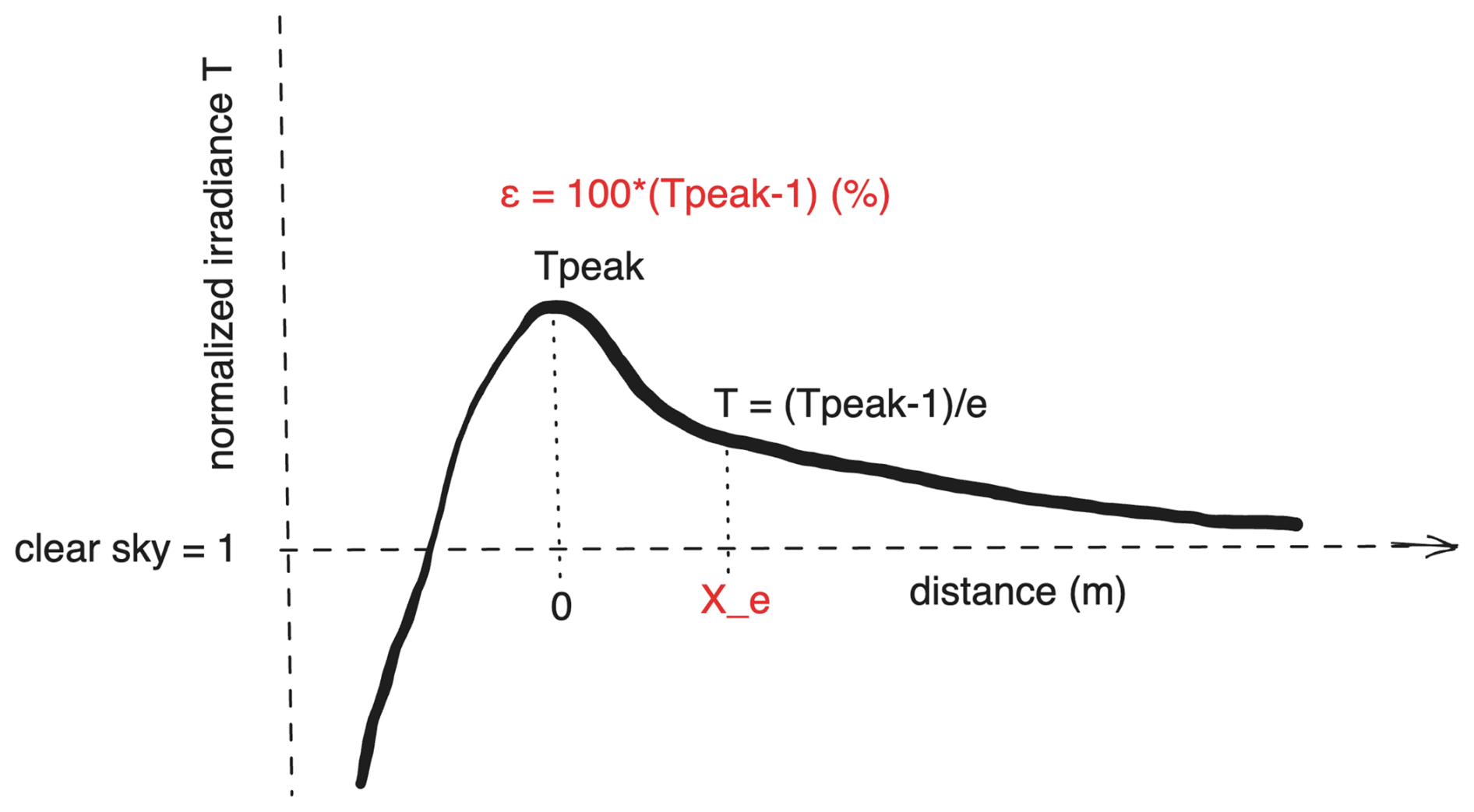
Figure 5 Sketch of the modified Lennard-Jones (exp,6) potential function (Eq. 2), highlighting ϵ the maximum potential peak (T_peak) and x_e the e-folding distance from the peak as parameters of interest. The function is modified so that the x axis is centred on the peak maximum and the values, relative to clear sky, approach the value 1, so that ϵ equals CE in percent.

The shape of the function is modulated by α and σ, where α describes the steepness of the dimming on the right side and σ modulates the width of the peak. From manual inspection compared to observed transition signatures, we set α to a value of 0.2. To centre Eq. (2) on the peak, the location of the extremum (x_m) is calculated by finding the root of its derivative:

$$\begin{array}{}\text{(4)}& \begin{array}{rl}{x}_m& =-{\displaystyle \frac{\mathrm{70}\mathit{\sigma }}{\mathit{\alpha }}}\mathrm{LambertW}\left(-{\displaystyle \frac{\mathit{\alpha }\exp (-\frac{\mathit{\alpha }}{\mathrm{7}})}{\mathrm{7}}}\right)\\ & =\mathrm{10}\mathit{\sigma }\mathrm{for}\mathit{\alpha }<\mathrm{7},\end{array}\end{array}$$

The e-folding distance is approximated from:

$$\begin{array}{}\text{(5)}& T\left(x_e\right)=\mathrm{1}+{\displaystyle \frac{T\left(x_m\right)-\mathrm{1}}{e}}=\mathrm{1}+{\displaystyle \frac{\mathit{ϵ}}{\mathrm{100}e}},\end{array}$$

as follows:

$$\begin{array}{}\text{(6)}& x_e=-{\displaystyle \frac{\mathrm{10}\mathit{\sigma }}{\mathit{\alpha }}}\ln \left({\displaystyle \frac{\mathrm{1}-\mathit{\alpha }}{e}}\right)\end{array}$$

We are able to fit Eq. (2), centred by x_m, to each observed transition signature to determine ϵ and σ by the curve_fit algorithm of the SciPy package (Virtanen et al., 2020). From the results of the fit we calculate x_e from Eq. (6). An example fit is shown in Fig. 10.

3.3 Feature importance analysis

We analyse the importance of externally measured variables for the derived ϵ and x_e parameters (see Sect. 3.2). As an initial step, we divided the data into several bins for three different external variables and applied the Virtanen et al. (2020) SelectKBest feature selection algorithm. Because our data set is relatively small compared to the large number of external variables, we constrained each feature-selection run to three variables at a time, each split into three bins. We then evaluated all possible combinations of three variables drawn from the entire set of external measurements. The choice of triplets is somewhat arbitrary, but provides a compromise between exploring a wide range of combinations and maintaining sufficient statistical robustness.

The SelectKBest method returns univariate F-test scores that quantify the linear dependence between each external variable and the target for a given triplet of variables. We consider scores larger than 0.3 to be significant. For each variable, we record how often it achieved a significant score in all combinations in which it appears. These frequencies are finally expressed as a percentage of significant occurrences per combination and are reported in Sect. 4.2.2. This metric indicates which variables are most suitable for parametrisation when the model is restricted to three variables. The objective is to demonstrate a systematic approach to constructing a parametrisation of transition signatures.

4 Results and Discussions

The selected case days with shallow cumulus clouds were used to study the characteristic signatures of cloud shadow transitions in the PyrNet observations during the S2VSR campaign. For example, during 13 June 2023 (shown in Fig. 3), shallow cumulus clouds are forming in the morning and continuously increase in cloud depth and form larger clusters until the afternoon. These clouds are relatively small in size; therefore, the common GHI signature frequently alternates between low and high values throughout the day due to the passage of several cumulus clouds (as also sketched in Fig. 4).

During a cloud gap, that is, in between two cloud shading events, the GHI is strongly enhanced compared to clear sky as shown in Fig. 3, where noon GHI values are about 20 % larger in cloud gaps than the reference clear sky values. Cumulus clouds appear around 16:00 UTC and can be identified by the resulting bimodal distribution of GHI that persists for the rest of the day. From 19:00 to 20:00 UTC on this day a second layer of high-level clouds appears, evident by two maxima in both the shadow and the enhanced peaks, indicating that radiation enhancement and cloud shadow irradiance are dependent on cloud height. Multilayer cloud events are excluded from further analysis in this study, as long as they are identified from the COGS data, to focus exclusively on single cloud shadow transitions.

Radiation enhancement can occur as a result of increased diffuse irradiance produced by reflections at nearby cloud edges (side-escape). Consequently, the side-escape mechanism is likely the dominant factor controlling the e-folding distance x_e on the bright side of the transition signature function (Eq. 2). For optically thin clouds with cloud optical depth (COD) below 10, radiation enhancement may also arise in the direct irradiance due to the pronounced forward-scattering characteristics of cloud droplets (forward-escape). The forward-escape mechanism likewise affects the e-folding distance by shaping the sharpness of the enhancement peak and strongly depends on the droplet scattering phase function, which is in turn governed by their effective radius. We do not account for phase (ice versus liquid) in this work, as we concentrate on shallow cumulus clouds with negligible ice content. Both forward- and side-escape mechanisms modify the bright side of the transition signature and are therefore expected to exert the strongest influence within the scope of our investigation. As shallow cumulus clouds rapidly deepen and attain COD values exceeding 10, the side-escape mechanism likely shows the strongest influence. The two mechanisms, albedo-enhancement and downward-escape, tend to increase diffuse irradiance within the shadow of the cloud. As a result, radiation levels may exceed clear-sky values near the cloud edge due to these processes, and the enhancement peak is extended further into the shadow region. The key parameters are the effective cloud droplet radius and COD for downward-escape and surface albedo for albedo-enhancement.

To study cloud shadow transitions in more detail, we analysed the selected signatures in two distinct ways: in Sect. 4.1, we evaluate GHI against the distance to cloud and cloud shadow mask edges using COGS data (refer to Sect. 2.2). This approach introduces 2D information that is not available from PyrNet time series alone, allowing us to determine the nearest shadow edge distance. However, this method is confined by the COGS product's resolution (20 s and 50 m), resulting in the smoothing of the transition signatures within a 50 m range. Interpolation between COGS time steps may compound this effect, and small cloud gaps might be overlooked when obscured by surrounding clouds. However, this provides a comprehensive view of radiation enhancements and shadow irradiance related to cloud proximity. In Sect. 4.2, we focus solely on PyrNet data, analysing transition signatures based on the relative distance from the shadow edge using the derived flow vector (see Sect. 3.2). Here, the resolution depends entirely on PyrNet's temporal resolution, allowing for a finer analysis of these signatures. However, the absence of two-dimensional data leaves the precise location of the nearest shadow edge unverified. Accordingly, we target the region near the transition peak, hypothesizing that it is primarily influenced by the cloud whose shadow recently moved past the station.

To characterise specific cloud properties, we rely on the following externally observed variables: CBH, geometrical cloud depth, and shadow chord length, which constrain the geometrical extent of the cloud; COD and droplet effective radius, which represent the optical characteristics of the clouds. Additionally, the sunlight chord length and the cloud fraction of opaque clouds indicate how separated or clustered individual clouds are. The sun's position and the atmospheric water vapour content are also taken into account to better constrain each individual situation.

4.1 Signatures analysed with distance information from COGS

Transition signatures are shown and analysed versus the geometric horizontal distance to the mask edge in Figs. 6, 7, 8, and 9. This is achieved using the COGS cloud and shadow masks as 2D information for the calculation of the distance to the nearest cloud and shadow edge (see Sect. 2.2). Therefore, this analysis is tied to the temporal resolution of COGS. At every COGS time step, the GHI observation of PyrNet is supplemented with information on the distance and direction to the nearest cloud and shadow edge.

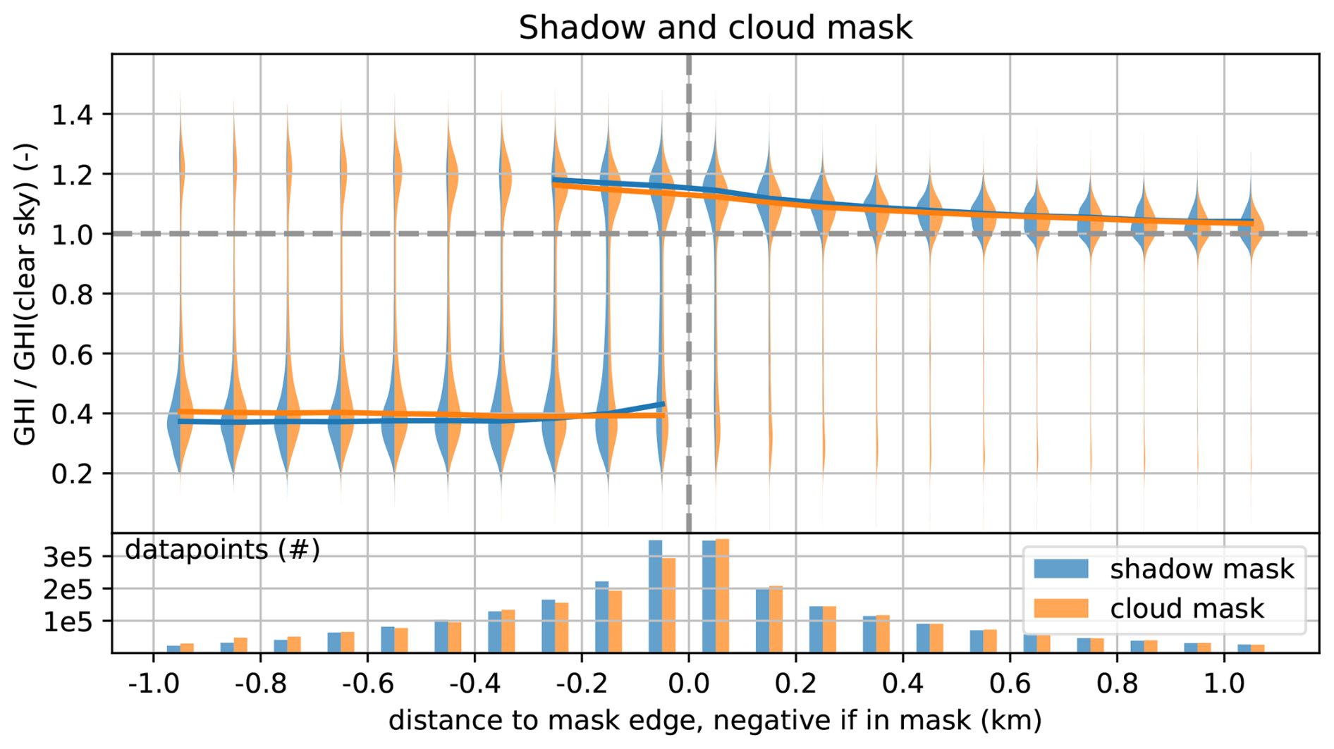
Figure 6 The violin plots showing observed GHI to clear sky GHI ratios for 100 m bins of distance to the respective cloud (orange) or shadow (blue) mask edge. Negative distances indicate that the data sample takes place inside the mask, meaning within the shadow or vertically below a cloud. In addition, the number of available data-points for each bin is shown.

The GHI observations are then aggregated into distance bins and are shown relative to their modelled clear sky reference value. The x-axis shows the horizontal distance to the corresponding mask edge, which means the edge of the cloud shadow on the ground (shadow mask) and the edge of the vertical projected cloud on the ground (cloud mask). Bins at negative distance values show observations from inside the mask, meaning within the cloud shadow (shadow mask) or vertically below a cloud (cloud mask). Inversely, bins at positive distance show observations in direct sun light (shadow mask) and in distance to a vertically projected cloud object (cloud mask). These analyses are bound to the COGS resolution; therefore, the data is displayed in 100 m bins to even out edge effects due to the 50 m COGS resolution. The violin plots in each figure panel are always two-fold for direct comparison, either comparing observations in distance relative to shadow or cloud mask (Fig. 6) or with respect to the shadow mask but splitting the data with reference to an external observation, such as CBH (Figs. 7, 8, and 9).

As shown in Fig. 6, focusing on the shadow masks, there is an approximately 20 % increase in radiation near the edge of the cloud shadow. This radiation enhancement peaks closest to the cloud shadow, but is already noticeable at roughly 1 km from the cloud shadow, indicating significant 3D-radiative effects, due to the side-escape mechanism (e.g., Mol and Van Heerwaarden, 2025). Moreover, the most pronounced enhancement is found in the −100 to −200 m bin, which may stem from small gaps in the cloud cover, especially near cloud edges, that are not captured by the cloud mask because of the COGS resolution. In addition, cloud edges are optically thin, so the forward-escape mechanism enhances radiation through pronounced forward scattering in these edge regions.

In the cloud mask in Fig. 6, the transition pattern resembles that of the shadow mask, yet it reveals increased radiation even when observations are directly underneath the cloud. This is clearly due to shadow displacement caused by the angle of solar incidence, yet these scenarios interestingly show the most substantial radiation enhancement. The significant increase in radiation beneath a cloud in direct sunlight strongly indicates 3D radiative effects, whether through downward- or forward-escape, or albedo enhancement mechanisms.

In Fig. 7, we only consider the shadow mask to analyse transition signatures and their dependency on the sun to cloud geometry, and in Figs. 8 and 9 on external observations of CBH, COD, cloud fraction and cloud droplet effective radius.

4.1.1 Dependence on sun-cloud geometry

Mol and Van Heerwaarden (2025) studied radiation enhancement for shallow cumulus clouds and found that the peak enhancement varies significantly with sun-cloud geometry. Their simulations focused on the side-escape mechanism, setting the surface albedo to zero. They found that the radiation enhancement peak is more pronounced on the sunlit side of the cloud and that this effect also depends on cloud depth. As the cloud depth decreases, the enhancement in radiation becomes weaker, though the sunlit side still remains significantly brighter than the shaded side. For instance, they reported roughly a 5 to 10 times stronger enhancement on the sunlit side of cumulus clouds with a depth of 500 m. In our case, the mean cloud depth is approximately 300 m. However, in our observations shown in Fig. 7a, these findings could not be replicated. We evaluated two data set selections: one on the shaded side, where the sun shares azimuthal alignment (±10°) with the cloud edge (blue violins), and another on the sunlit side, in the opposite azimuthal direction (orange violins). Our observations did not reveal significant radiation enhancement differences between the sunlit and shaded sides, probably due to the combined effects of side- and forward-escape and albedo phenomena. Natural clouds exhibit greater fractal complexity compared to idealised simulations, which can improve forward-escape, as suggested by Mol and Van Heerwaarden (2025). In addition, albedo was not considered in their research, but it can have a substantial impact (e.g., Gueymard, 2017; Villefranque et al., 2023). Apart from similar peak magnitudes of radiation enhancement on the sunlit and dark side of the cloud, radiation enhancement is slightly stronger at the lit side for all distance bins. This indicates still stronger side-escape effects on the lit side and is consistent with Mol and Van Heerwaarden (2025). Interestingly, the region under cloud shadow near the sunlit side appears considerably brighter than the shaded area, with radiation enhancement extending further within the cloud (see −200 to −100 m bin). This finding underscores the importance of the forward-escape and albedo-enhancement mechanisms which enhance diffuse irradiance in the shadow region in comparison to shadows close to the dark side of the cloud. We sought to differentiate between these effects by focussing on cases with a COD exceeding 15 in Fig. 7b, ensuring forward-escape impacts are confined to the edge of the cloud depending on solar incidence. The outcomes closely mirror Fig. 7a, though shadow irradiance near the sunlit side showed a slight increase, highlighting the notable influence of the albedo-enhancement.

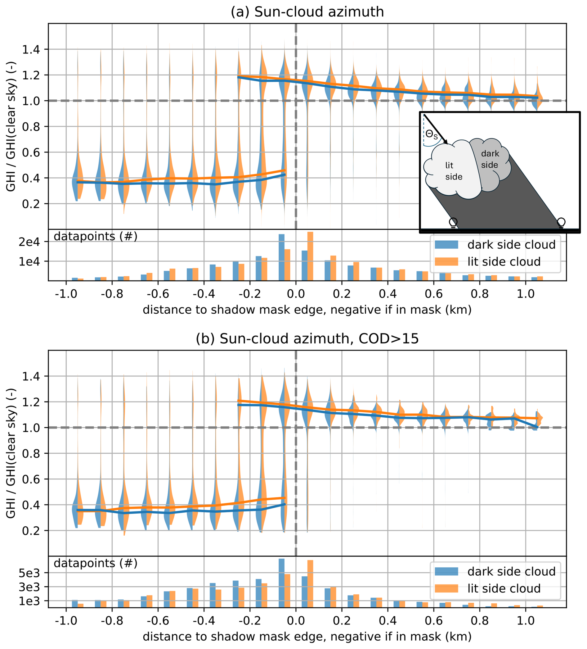
Figure 7 As Fig. 6 but orange and blue now refer always with respect to the cloud shadow mask. (a) Sun–cloud azimuth angle indicating the sample was taken close to the dark side of the cloud (blue, cloud shadow and solar azimuth are in the same direction), and the lit side of the cloud (orange, cloud shadow and solar azimuth are in opposite directions). Panel (b) is similar to panel (a) but limiting the data set to thick clouds of COD larger than 15 to reduce enhancement effects due to forward- and downward-escape.

4.1.2 Dependence on externally observed variables

In the following we examine transition signatures with respect to externally observed variables as depicted in Fig. 8. The threshold used to partition the data set is determined to ensure an approximately equal number of data points in each half.

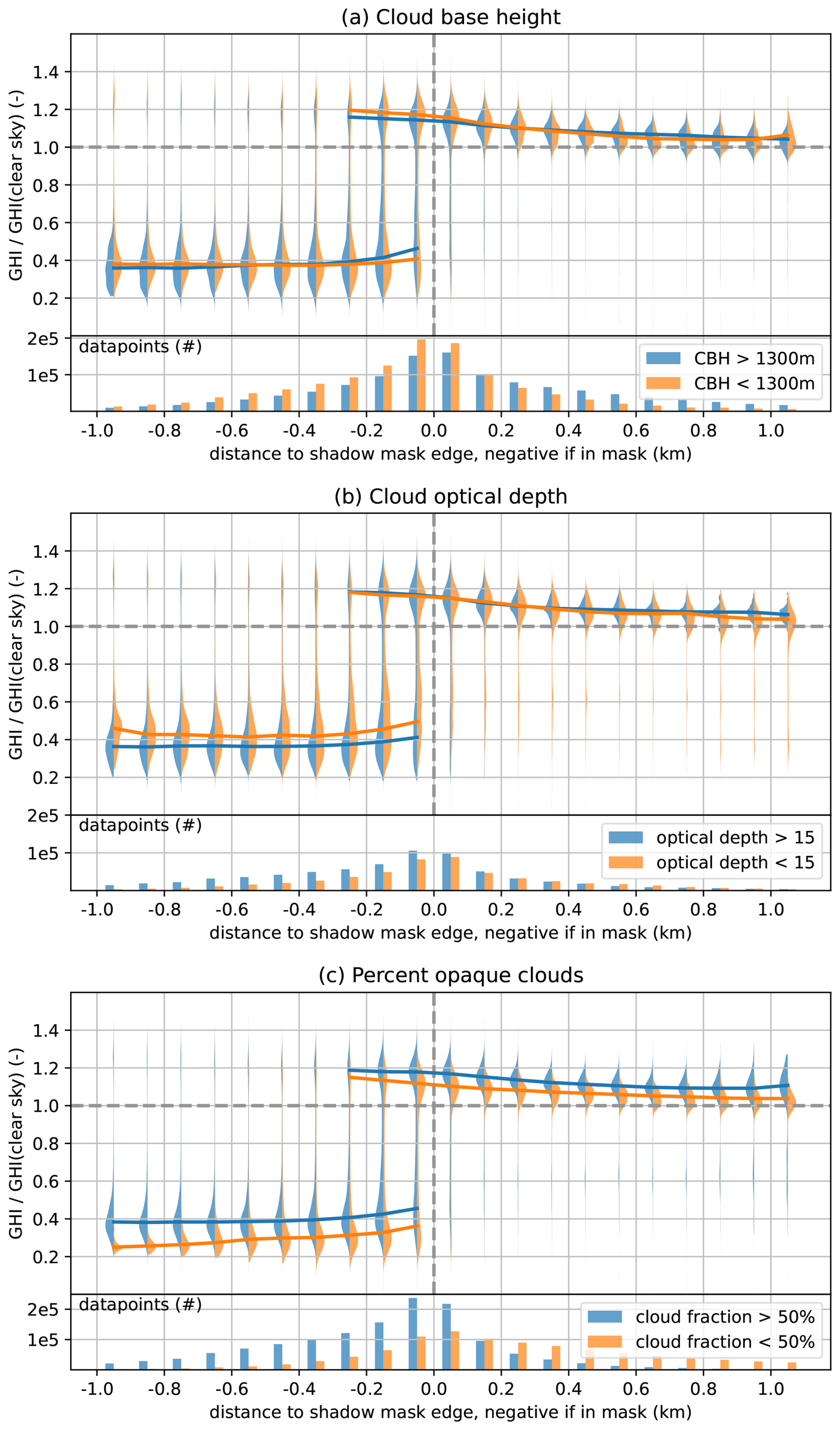
Figure 8 As Fig. 7 but for a different selection of external variables. Blue and orange violins indicating samples at respectively low and high values of cloud base height (a), cloud optical depth (b), and cloud fraction of opaque clouds (c).

Investigating the transition signatures with respect to CBH, we found lower peak values of radiation enhancement for higher clouds (Fig. 8a). This is intuitive from a geometric perspective, as higher clouds spread solar radiation to a wider area by side-escape. In addition, radiation enhancement is found slightly deeper into the shadow, even within the -300 to -200 m bin, which also indicates a wider spread granting a similar forward-escape effect. Due to the albedo-enhancement, one would expect brighter shadows from lower clouds (He et al., 2024), but up to the −500 to −400 m bin into the cloud shadow this is probably compensated in our observations by side-escape effects from other nearby clouds in the scene. Deeper into the shadow, the observation shows brighter shadows from lower clouds, as expected from the albedo-enhancement.

The COD (Fig. 8b) has only minor effects on radiation enhancement. This agrees with the findings of He et al. (2024) for liquid water content, where variations of ±40 % in liquid water content resulted in changes in GHI within shadow and enhancement regions of only about ±10 W m⁻². Obviously, shadows are brighter when the clouds are more translucent. Interestingly, there are several observations of shadow in bins from 500 to 1100 m showing that the COGS mask occasionally misses a cloud when it is optically thin.

He et al. (2024) found from their sensitivity studies that increasing cloud cover results in brighter shadows and more intense radiation enhancement close to the cloud shadow, as cloud gaps are smaller and therefore the side-escape effect impacts neighbour cloud shadows and the overall radiation enhancement in the area. Comparing the transition signatures with the TSI cloud fraction for opaque clouds in Fig. 8c leads to the same conclusion, supporting their findings of an increase in GHI of more than 50 W m⁻² in shadow and enhancement situations as the cloud shadow fraction rises from about 10 % to 20 %.

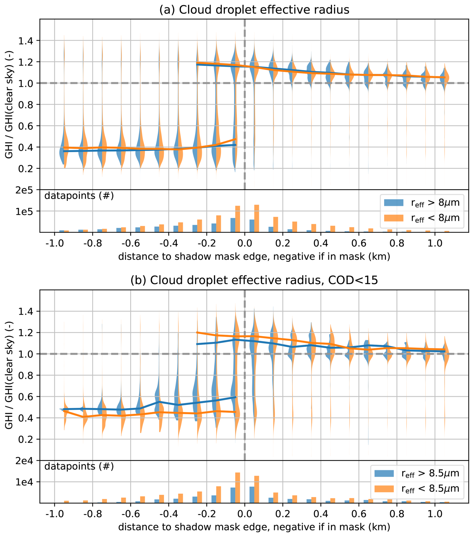
Figure 9 As Fig. 7 but blue and orange violins indication samples at respectively low and high values of cloud droplet effective radius. In panel (b) the data set is limited to thin clouds of COD lower than 15 to reduce the influence of side-escape and albedo-enhancement.

The lower effective radius of the cloud droplets leads to a higher cloud albedo and therefore should increase the albedo-enhancement and side-escape. In Fig. 9a deep shadows are brighter due to albedo-enhancement and close to the edge of the shadow, the increased forward-escape due to the stronger forward scattering of the larger droplets competes with the stronger side-escape from the nearby clouds. When the data set is limited to thin clouds (COD < 15), stronger forward-escape by larger cloud droplets becomes evident by the brighter overall shadows, while the enhanced side-escape of the smaller droplets is indicated by a stronger radiation enhancement close to the cloud shadow (see Fig. 9b).

4.2 Signatures analysed with distance relative to flow

Focusing in greater detail on the radiation enhancement peak close to the cloud shadow, we analyse the transition signatures identified by PyrNet as a function of the distance to the cloud shadow edge, derived from the flow vector. In this part of the analysis, we use only PyrNet measurements, supplemented by flow information. The high temporal resolution enables for a more detailed examination of the signature peaks. Because two-dimensional information is not used in this part of the study, we restricted the analysis to a small area around the transition peak, which is predominantly affected by the cloud whose shadow has just passed over the station. The identified transition signatures are fitted to obtain the two parameters ϵ and x_e, which represent the amplitude of the enhancement peak and the e-folding distance, respectively. In a second step, variations in external observed variables are compared with ϵ and x_e to assess their statistical feature importance, working towards a parametrisation of cloud shadow transition signatures.

4.2.1 Transition signature fit

Radiation enhancement is most prominent near the edge of the cloud shadow. When there is a shadow gap, the radiation values approach the radiation enhancement level. From 5 d with shallow cumulus clouds in the S2VSR campaign (Sect. 2), we detected 8931 transition signatures (Sect. 3.1) and presented them in a 2D histogram plot relative to the radiation enhancement (Fig. 10). For uniform comparison, all signatures are aligned at their peak and flipped so that the cloud shadow is consistently on the left. In this representation, the x-axis represents the distance with respect to the flow from the peak location. A pronounced increase in GHI can be observed at the edge of the shadow, about 2 % higher than the prevailing enhancement level. This rise could stem from side- or forward-escape, influenced by the solar beam's incident angle and COD, potentially extending into the projected shadow region for the latter. Due to the centring on the peak, this analysis does not differentiate these factors.

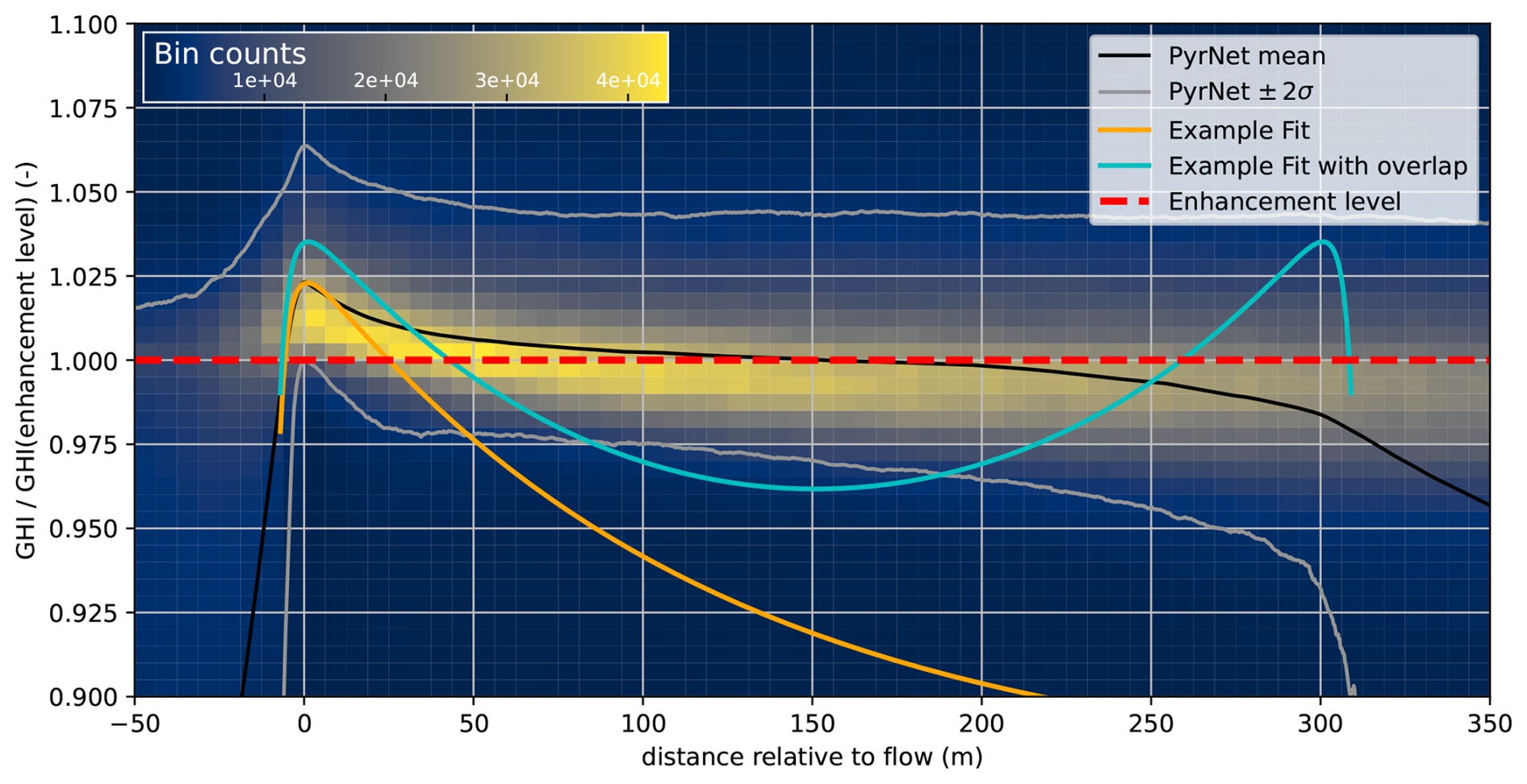
Figure 10 Histogram of all 8931 selected transitions signatures from PyrNet observations from 5 d with shallow cumulus clouds. Bright colors indicate bins with high number of samples. The data is shown relative to the enhancement level (red, dashed) in between cloud shadow gaps. The PyrNet mean value (black) approaches this value, while the example fit (orange line) of Eq. (2) approaches the respective clear sky value (outside of plot range). The cyan line shows the same fit, but with overlapping the inverted function simulating a nearby cloud with a distance of 300 m.

To examine the shape of the transition signature, we are particularly interested in the amplitude of the enhancement peak (ϵ) and the steepness of the peak as a measure of how far 3D effects from one cloud influence the point of observation. Therefore, we fitted Eq. (2) to each individual transition as described in Sect. 3.2, focusing on 30 m around the peak. In Fig. 10 the orange line shows a fit of one transition signature from the data set. Note that it starts to deviate strongly from the observational mean shortly after the peak because this function is designed to approach the clear sky radiation level at some point, which would be the case for an isolated cloud. In reality, multiple clouds influence the observations, so the mean transition signature approaches the radiation enhancement level because of the overlapping signatures. This is simulated by the cyan line in Fig. 10, where we show two overlapping signatures with a peak distance of 450 m. Overlapping of fit functions could potentially be used to infer cloud gap size if Eq. (2) can be parametrised well, and we assume similar cloud properties in the present cloud field. It is beyond the scope of this study to evaluate this approach, but it is a potential follow-up in the future.

4.2.2 Feature importance

To examine the dependence of ϵ (amplitude of enhancement) and x_e (e-folding distance of the enhancement) of Eq. (2) to several external observed variables, such as CBH, COD and droplet effective radius from the ARM data, we show the absolute Pearson correlation in Fig. 11a and b. Since the specific side of the cloud facing the sun is irrelevant, we can calculate the correlation for the sun to cloud azimuth angle by first normalizing it to a range of 0 to 180°. This is achieved by taking the absolute values for the range of 0 to −180°. In addition to Fig. 11, Fig. 12 shows the absolute changes of ϵ and x_e compared to these external observed variables.

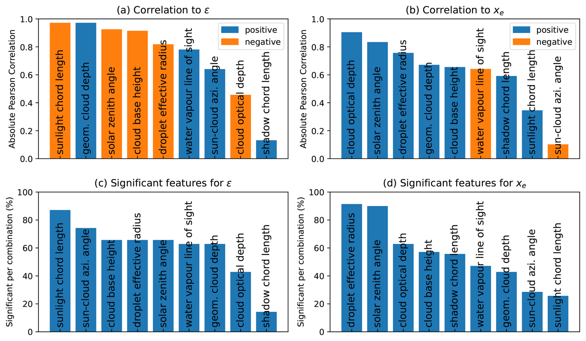
Figure 11 Feature absolute correlation and sign indicated by colours (a, b) and percentage of combinations of three features where a specific feature is significant (c, d) for cloud shadow transition signature parameters ϵ (a, c) and x_e (b, d).

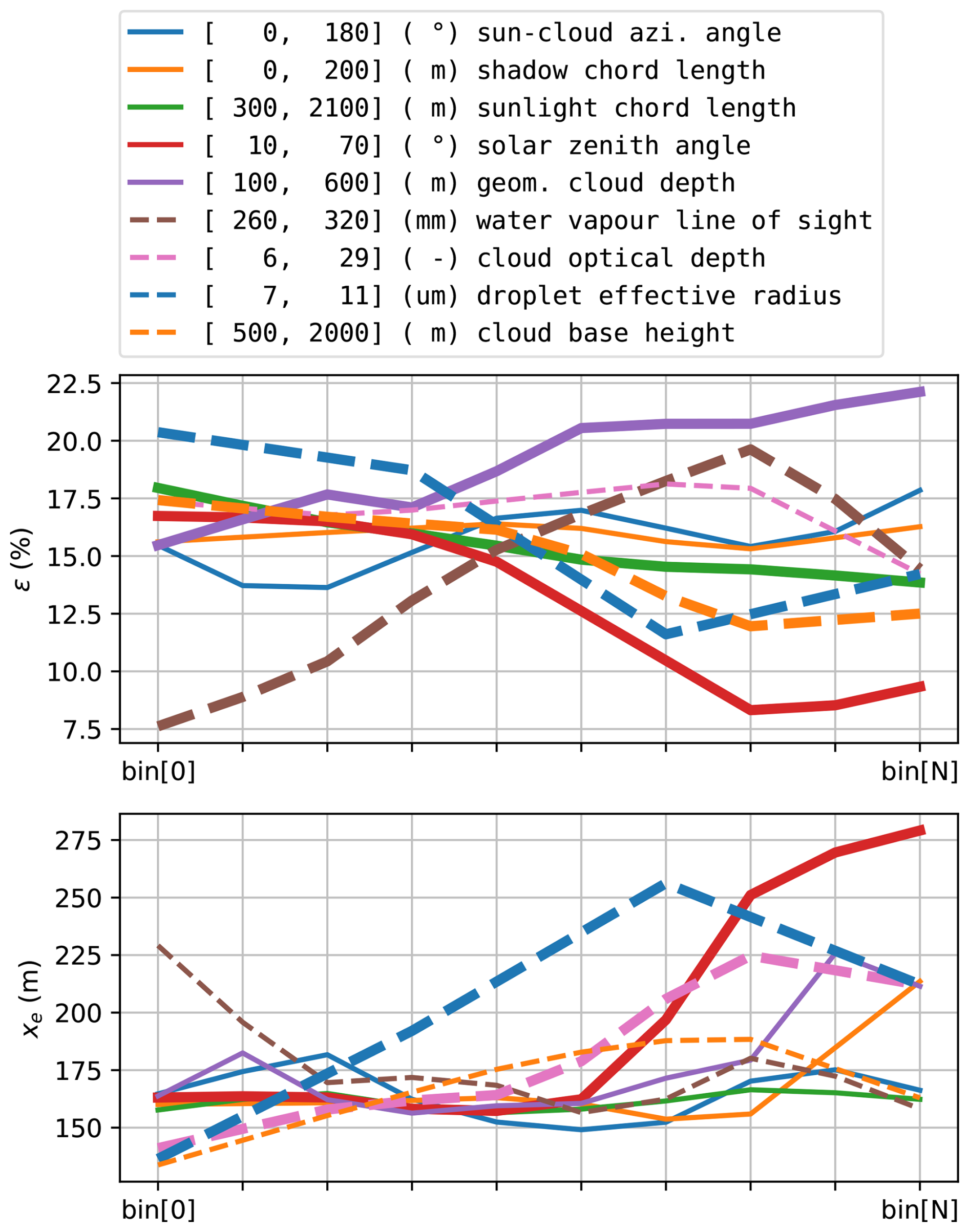
Figure 12 External features in comparison to ϵ and x_e, shown in a standardized binned representation. The legend of the figure indicates the range and units of the features. Lines are drawn with increased thickness if the linear correlation with ϵ and x_e exceeds 0.75.

In addition, for several combinations, each of three different external observed variables, we performed a feature importance analysis for variables in the respective combination, as described in Sect. 3.3. Figure 11c and d show the percentage of combinations where a specific variable has a significant dependency. The correlation indicates a direct linear dependency on the individual variables. Significance per combination, on the other hand, gives insight into which variables to choose for parametrisation if one limits the model to three variables. Therefore, the significance per combination can differ from the linear correlation for certain features.

The length of the sunlight chord shows a strong correlation with the amplitude of radiation enhancement (ϵ). Even if the sunlight chord length is only the 1D representation of cloud gap size, it resembles the cloud gap size information well. Smaller gaps between clouds cause greater overlap of transition signatures from side-escape, so the sunlight chord length is inversely related to ϵ. We find that ϵ decreases from roughly 18 % to 13 % as the sunlight chord length increases from 300 to 2100 m (see Fig. 12). As the size of the cloud gap does not effect the cloud albedo or the scattering function, a weak correlation is shown to x_e. So we found the sunlight chord length to be the most significant feature for ϵ and the least significant for x_e.

Similarly, other geometric variables, namely geometric cloud depth, solar zenith angle, cloud base height, shadow chord length, and the sun to cloud azimuth angle, show strong correlation with ϵ and less with x_e. There are three notable exceptions: The strong correlation of the solar zenith angle with x_e, since a flat angle of incidence increases reflection at the edge of the cloud. Second, the azimuth angle of the sun to the cloud is the weakest correlated variable among the geometric variables with respect to ϵ, as already found in Sect. 4.1 due to opposing enhancement mechanism and overall low geometric cloud depths. Third, the shadow chord length is only weakly correlated to both ϵ and x_e and therefore ranks very low according to significance. The size of the shadow doesn't matter much, but the distribution and optical properties of the cloud do. In our comparison, however, we were only able to present cases with relatively short cloud shadow chord lengths of up to 200 m (see Fig. 12), because situations with longer chords were rare and did not allow for statistically robust analysis.

Optical and microphysical properties of the clouds directly influence extinction of sunlight at the cloud, and so the radiation enhancement mechanisms. Although COD is not strongly correlated to ϵ as found also in Sect. 4.1, it does affect the broadness of the transition peak, so it is brighter from further away due to enhanced side-escape by higher COD values. The effective radius of cloud droplets affects the scattering function, leading to a negative correlation to ϵ as smaller droplets enhance cloud albedo and therefore the enhancement peak amplitude due to enhanced side-escape. Similarly, it shows a positive correlation to x_e, meaning a sharper enhancement peak from small droplets. This could be explained by a stronger separation of forward- and side-escape when cloud droplets are big and therefore show strong forward scattering, so forward-escape is more confined to within the projected shadow area and side-escape close to the shadow edge, while for smaller droplets both effects will overlap to a certain extent, leading to a sharp enhancement peak. As shown in Fig. 12, ϵ drops from about 20 % to 13 %, meanwhile the e-folding distance x_e increases from 140 to 220 m when the droplet effective radius changes from 7 to 11 µm.

Finally, we can summarise that to parametrise the transition signature of radiation enhancement, one needs to consider information from both geometrical and microphysical properties of the present cloud situation. If one had to choose a limited set of external variables to describe transition signatures for shallow cumulus clouds, one would start with the variables of highest significance shown in Fig. 11. The size of the cloud gap, the azimuth angle of the sun to the cloud, and the CBH are the most significant features regarding the peak enhancement amplitude. The droplet effective radius, solar zenith angle, and COD, on the other hand, are significant to describe the sharpness of the enhancement peak.

5 Conclusions, Summary and Outlook

In this study, we successfully combined radiation measurements and stereo reconstruction of clouds to study 3D radiative effects in the vicinity of clouds on an observational basis.

We examined characteristic signatures of cloud shadow transitions in high-temporal resolution time series of GHI as observed by PyrNet, a spatially dense pyranometer network. PyrNet was deployed at the ARM-SGP site in Oklahoma, USA, in summer 2023 during the S2VSR field campaign. We used the 4D COGS cloud mask derived from a stereoscopic cloud reconstruction for shadow identification, together with other routine ARM-SGP observations. Due to the high number of stations and network layout, PyrNet in synergy with COGS provided a unique data set of densely-sampled high temporal resolution GHI measurements and collocated cloud information. The quality and comparability of these time series were ensured through careful cross-calibration and cosine correction.

Our analysis concentrates on shallow cumulus cloud events during five selected case days of S2VSR, comprising a total of 550 hours of GHI observations during the daytime. Transition signatures were identified by comparing values against the simplified Solis clear sky model and identified by events of strong GHI slope. The signatures were temporally aligned to the exact time of transition and were subsequently converted to distances using cloud motion. The latter was calculated using flow vectors derived from the COGS cloud mask through the Farnebäck optical flow algorithm. Each signature was fit with a modified Buckingham (exp,6) potential function to determine the amplitude of the radiation enhancement and the e-folding distance, capturing the magnitude and sharpness of the transition.

We can summarize the key results as follows:

• The PyrNet setup enables clear resolution of cloud-shadow transition signatures.

• Observed data reveal radiation enhancement at cloud edges due to 3D radiative effects.

• The transition signature has been quantitatively characterized in this study. To parametrise the cloud-shadow transition signature, we examine how the observed signatures are affected by several different features.

• The peak amplitude of CE was approximately 2 % above the baseline enhancement level and 20 % above clear sky values. It is strongly influenced by:

  • cloud (shadow) gap size

  • cloud base height

  • sun-cloud geometry

• The maximum e-folding distance (a measure of the maximum sharpness) is approximately between 160–180 m and depends on:

  • cloud droplet effective radius

  • cloud optical depth

  • solar zenith angle

Consequently, we conclude that both geometric and microphysical cloud properties influence the cloud shadow transition signatures, and encourage their consideration in parametrisations of cloud shadow transition signatures. Dense observational networks such as PyrNet are essential for constraining such parametrisations. These parametrisations could be applied, for instance, in PV sensitivity analyses by artificially generating GHI time series from a clear sky model together with a distribution of shadow gap lengths defined by a specified cloud fraction and cloud size distribution. At the shadow edges, the parametrised transition signatures can be used to create time series with enhanced radiation.

This analysis was made possible by the number of pyranometer stations during the field campaign, in combination with the high sampling rate achieved using photoelectric pyranometers. A standard setup of one station with thermoelectric pyranometers would not be able to resolve the signatures because of their delayed response time and the low number of observable transition signatures in a few case days.

In our study, we limited our focus to shallow cumulus clouds over 5 d during S2VSR. We plan to extend this method to a larger data set that incorporates over a decade of PyrNet data from multiple field campaigns. Expanding this characterisation to other cloud regimes represents a further worthwhile step towards parametrising CE from observations. The integration of PyrNet and COGS data from the S2VSR campaign offers a valuable resource for research focused on the alignment and consistency of ground-based radiation measurements with high-resolution satellite imagery and products, such as those from the GOES-R ABI geostationary sensor and the Sentinel-2 MSI imager. Additionally, the analysis of tilted irradiance observed at PyrNet stations is particularly relevant to studies on photovoltaic energy output.