Mechanisms of air–sea CO₂ exchange in the central Baltic Sea

Air–sea gas exchange regulates the cycling of climate-relevant gases such as carbon dioxide (CO₂), yet significant uncertainties remain in its quantification. The gas transfer velocity (K), a key parameter for estimating CO₂ flux, is usually expressed as a function of wind speed (U_10N). This approach overlooks the role of fetch and surfactants, which can substantially affect K. However, no field study has systematically quantified their combined effects under fetch-limited and surfactant-abundant ocean conditions. To fill this research gap, we conducted air–sea gas exchange studies during a cruise in the central Baltic Sea, a system with high surfactant levels and a short fetch. We report independent determinations of K using eddy covariance (EC) and dual-tracer (${}^{\mathrm{3}}\mathrm{He}/{\mathrm{SF}}_{\mathrm{6}}$) techniques, together with direct measurements of natural surfactants and modelled wave parameters. Both methods yield consistent results; however, EC-based CO₂ transfer velocities are, on average, 33 % lower than those reported in previous EC studies in the open ocean. Sea-state-dependent parameterisations indicate that limited fetch reduces K by 8 %, while elevated surfactant concentrations may have contributed to the additional 25 % reduction. We developed an updated parameterisation that includes wind stress, sea state, and surfactants. When applied to climatological forcing, it yields a 40 % stronger seasonal cycle (greater oceanic uptake during summer and enhanced outgassing during winter) of CO₂ flux in the Baltic Sea than obtained with the conventional U_10N-based parameterisation. These findings highlight the need to move beyond U_10N in parameterising K and estimating regional fluxes, especially when evaluating the potential of marine carbon dioxide removal (mCDR) in coastal seas.

1 Introduction

The ocean is a major sink of carbon dioxide (CO₂) emitted by human activities, substantially mitigating climate change (Friedlingstein et al., 2025). Beyond its natural carbon uptake capacity, marine-based carbon dioxide removal (mCDR) has emerged as a climate mitigation approach under ongoing global warming (Doney et al., 2024). Accurate quantification of global ocean carbon flux and the regional mCDR efficiency is essential for climate predictions. Air–sea CO₂ flux is often estimated using the bulk formula:

$$\begin{array}{}\text{(1)}& F=K_{\mathrm{660}}{\left({\displaystyle \frac{\mathit{Sc}}{\mathrm{660}}}\right)}^{-n}({\mathit{\alpha }}_{w}f{\mathrm{CO}}_{\mathrm{2}w}-{\mathit{\alpha }}_{i}f{\mathrm{CO}}_{\mathrm{2}a})\end{array}$$

where F ($\mathrm{mmol}{\mathrm{m}}^{-\mathrm{2}}{\mathrm{d}}^{-\mathrm{1}}$) is the air–sea CO₂ flux, K₆₆₀ (cm h⁻¹) is the gas transfer velocity normalized to a Schmidt number (Sc) of 660, corresponding to CO₂ in seawater at 20 °C. The value of the exponent n is between $\mathrm{1}/\mathrm{2}$ and $\mathrm{2}/\mathrm{3}$ (Jähne et al., 1987), and is often assumed to be $\mathrm{1}/\mathrm{2}$ in the ocean environment (Wanninkhof et al., 2009). CO₂ solubilities (e.g., $\mathrm{mol}{\mathrm{L}}^{-\mathrm{1}}{\mathrm{atm}}^{-\mathrm{1}}$) at the base of the mass boundary layer and at the air–sea interface are α_w and α_i, respectively. CO₂ fugacity (fCO₂, µatm) at these locations is fCO_2w and fCO_2a. Sc and α depend on water temperature and salinity (Wanninkhof, 2014; Weiss, 1974). Notably, if both the CO₂ flux and fCO₂ are known, K₆₆₀ can be derived.

Equation (1) highlights the central role of K₆₆₀ as the kinetic forcing parameter in air–sea CO₂ exchange. K₆₆₀ is directly driven by near-surface turbulence (Garbe et al., 2014). On a global scale, wind forcing has a dominant effect on gas transfer velocity, and other factors, such as friction velocity, waves, and bubbles, are strongly linked with wind speed (Wanninkhof et al., 2009). Thus, the readily available 10 m neutral wind speed (U_10N) is often used as the sole variable for parameterising K₆₆₀ (e.g., Ho et al., 2006; Nightingale et al., 2000; Wanninkhof, 2014). However, wind is not the only factor driving gas exchange, as other factors not fully linked to wind speed can substantially influence this exchange at regional scales, particularly in the coastal ocean (Upstill-Goddard, 2006). Existing U_10N-based K₆₆₀ formulations in the Baltic Sea yield controversial results (e.g., Gutiérrez-Loza et al., 2022; Kuss et al., 2004), highlighting the lack of mechanistic understanding of air–sea gas exchange.

Surfactants are surface-active compounds, molecules, or biomolecules. They are ubiquitous in the ocean and often highly concentrated in coastal waters through biological production and terrestrial inputs (Mustaffa et al., 2020; Sabbaghzadeh et al., 2017; Wurl et al., 2011), suppressing gas exchange by damping surface turbulence and forming an additional diffusion barrier (McKenna and McGillis, 2004; Pereira et al., 2016). In contrast, wave breaking enhances gas transfer, especially for low-soluble gases, by introducing bubbles as an exchange pathway in addition to the interfacial exchange route (Bell et al., 2017; Blomquist et al., 2017; Dong et al., 2025; Woolf, 1997). Wave breaking is strongly impacted by wind fetch (defined as the distance over which wind acts on the water surface), because limited fetch suppresses wave breaking and bubble generation (Fairall et al., 2006; Kunz and Jähne, 2018; Ocampo-Torres and Donelan, 1995; Prytherch and Yelland, 2021; Woolf, 2005). Understanding how these mechanisms influence air–sea gas exchange is essential for regional (coastal) carbon budgets and for developing robust monitoring, reporting, and verification (MRV) frameworks to support mCDR strategies (e.g., Ho et al., 2023).

The Baltic Sea, with its high summer primary productivity (Schmidt and Schneider, 2011) and limited fetch, provides an ideal natural laboratory for investigating the combined effects of surfactants and fetch on air–sea gas exchange. We therefore conducted a comprehensive gas exchange experiment in the central Baltic Sea to quantify the impact of factors additional to wind speed on gas exchange.

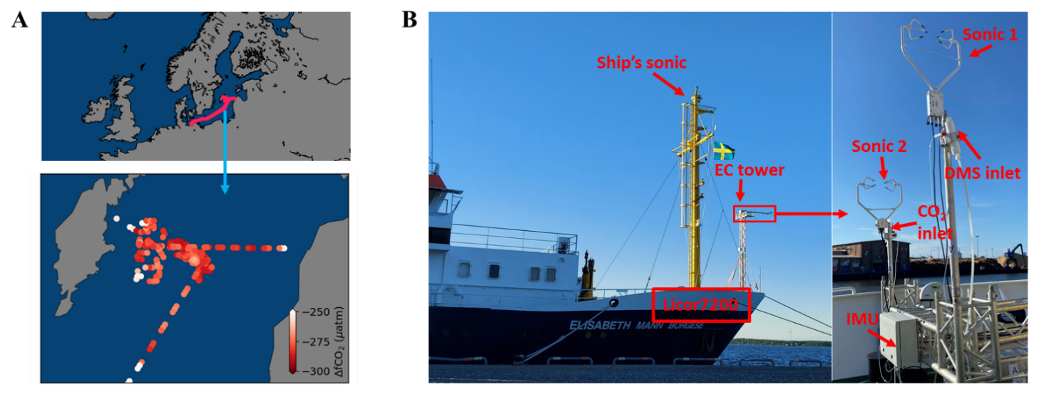
Figure 1 CenBASE cruise tracks and the ship-based eddy covariance (EC) system. Left panel: Cruise tracks in the central Baltic Sea, color-coded by air–sea CO₂ fugacity differences (ΔfCO₂). Middle panel: Research vessel EMB during the CenBASE cruise; a custom-built EC tower is mounted at the bow. Right panel: Instruments mounted on top of the tower, including sonic anemometers, a motion sensor (IMU), and the CO₂ inlet. Additional setup details are provided in Sect. 2.

2 Methods

2.1 CenBASE cruise

The Central Baltic Air-Sea Exchange Experiment (CenBASE; EMB 295) was conducted in summer 2022, immediately after the phytoplankton bloom season, to capture strong air–sea gas exchange signals (Parard et al., 2016; Bittig et al., 2024). The research cruise on the R/V Elisabeth Mann Borgese (EMB) departed from Rostock, Germany, on 2 July and returned on 18 July, with the primary study area located in the Gotland Basin (Fig. 1A).

Eddy covariance (EC) CO₂ flux observations (Sect. 2.2) and the ${}^{\mathrm{3}}\mathrm{He}/{\mathrm{SF}}_{\mathrm{6}}$ dual-tracer experiment (see Appendix A1) were performed simultaneously to determine gas transfer velocities, representing the second successful joint deployment of these two approaches after GasEx-98 (Ho and Wanninkhof, 2016; McGillis et al., 2001). Surfactant samples were collected from both the microlayer and underlying water (see Appendix A2). Wave parameters were extracted from the ERA5 hourly reanalysis data product (0.5° × 0.5°) (Hersbach et al., 2020) based on the cruise track's spatiotemporal coordinates. Additional measurements included fCO₂, sea surface properties, and meteorological variables to support the analysis.

2.2 Eddy covariance CO₂ flux measurements

The EC technique allows for direct measurements of air–sea CO₂ flux using the following equation:

$$\begin{array}{}\text{(2)}& F=\mathit{\rho }\stackrel{\mathrm{‾}}{w^{\prime }{c}^{\prime }}\end{array}$$

where ρ is the mean molar density of dry air (in mole m⁻³), w is the vertical wind velocity (in m s⁻¹), and c is the dry air mole fraction of CO₂ (in ppm or µmol mol⁻¹). The primes denote the fluctuations from the mean, and the overbar indicates time averaging. Due to the dynamic nature of the marginal sea environment, a 10 min averaging interval was chosen, shorter than the 20–30 min typically used in the open ocean (e.g., Blomquist et al., 2017). The CO₂ transfer velocity ($K_{\mathrm{660}\mathit{\_}{\mathrm{CO}}_{\mathrm{2}}}$) is derived by combining Eqs. (1) and (2). The EC momentum flux is similarly calculated as $\mathit{\rho }\stackrel{\mathrm{‾}}{w^{\prime }{u}^{\prime }}$, where u is the horizontal wind component. The friction velocity (u_∗) is then derived as the square root of the momentum flux divided by the air density.

Most components of the EC system were mounted on a custom-built tower at the bow of the ship to minimize the flow distortion (Fig. 1B). The tower extended 5 m above the deck, reaching a height of 14 m above mean sea level (a m.s.l.). A three-dimensional (3D) sonic anemometer (CSAT3B, Campbell Scientific) was installed on the starboard arm to measure the wind fluctuations, with a backup unit on the port side (CSAT3). An Inertial Measurement Unit (IMU, SBG Systems), housed in a meteorological box at the top of the tower, recorded ship motion. The IMU was positioned 66 cm from the starboard sonic and 173 cm aft of it. CO₂ fluctuations were measured using a LI-7200 gas analyzer. The sampled air was dried with a Nafion dryer operating in “reflux” mode (Perma Pure LLC). Air was drawn from the port-side inlet through a ∼ 10 m Teflon tube ($\mathrm{3}/\mathrm{8}$” inner diameter) at a stable flow rate of 33.2 ± 0.3 L min⁻¹, which results in turbulent flow within the tube. The 20 Hz signal from the sonic anemometer, IMU, and LI-7200 was logged by a datalogger (CR6, Campbell Scientific).

Data processing and quality control procedures followed those described in Dong et al. (2021). Briefly, motion corrections were applied to the wind (Edson et al., 1998; Miller et al., 2008) and CO₂ signals (Miller et al., 2010) to remove contamination from ship motion. A nitrogen puff test revealed a 0.3 s e-folding response time, which is used to correct the high-frequency attenuation (Blomquist et al., 2014). The time delay (∼ 2.5 s) between the inlet and the gas analyzer was assessed via the maximum covariance method. Flow distortion was minimized by mounting the EC tower arms beyond the ship's hull.

2.3 Auxiliary observations

The partial pressure of CO₂ in surface water was measured at 1 min intervals using the Mobile Equilibrator Sensor System (MESS) paired with two off-axis integrated cavity output laser spectrometers (oa-ICOS, Los Gatos Instruments) (Sabbaghzadeh et al., 2021). Seawater was continuously drawn from the ship's inlet at a depth of ∼ 3.3 m. Atmospheric CO₂ was measured daily using an air inlet mounted on the ship's foremast at 13.5 $\mathrm{m}\mathrm{a}.\mathrm{m}.\mathrm{s}.\mathrm{l}.$ These air CO₂ data are compared to the absolute CO₂ values measured by the EC gas analyzer (LI-7200, LI-COR, Inc.) to generate the 10 min time series of atmospheric CO₂. Sensor calibration was performed almost daily using standard gases from the Central Analytical Laboratories of the European Integrated Carbon Observation System (ICOS RI). Mean wind measurements were obtained from a sonic anemometer mounted 17 $\mathrm{m}\mathrm{a}.\mathrm{m}.\mathrm{s}.\mathrm{l}.$ on the ship's foremast to minimize flow distortion (O'Sullivan et al., 2013). Residual distortion was corrected using the ERA5 reanalysis wind product and nearby station records (see Appendix A3). Atmospheric pressure and temperature at ∼ 13.5 $\mathrm{m}\mathrm{a}.\mathrm{m}.\mathrm{s}.\mathrm{l}.$ were recorded by the onboard weather station. Surface seawater temperature and salinity were monitored by the ship's underway system and calibrated against CTD (conductivity, temperature, and depth) casts. A spar buoy equipped with cameras and sensors for temperature, salinity, and dissolved oxygen was deployed at several stations to characterize upper-ocean bubble and water column dynamics.

In addition, EC air–sea CO₂ flux observations from previous open-ocean cruises (Yang et al., 2022) are also used for comparison with the CenBASE results. Wave parameters were extracted from the ERA5 analysis wave product according to these open-ocean EC cruise tracks (see Yang et al., 2022) and the CenBASE cruise. The COARE model is used to estimate the bulk u_∗ (Edson et al., 2013). For the open-ocean scenario, environmental variables from the corresponding cruises are used as inputs to the COARE model (Yang et al., 2022). The environmental parameters observed during the CenBASE cruise are used to estimate the Baltic Sea u_∗ in the COARE model.

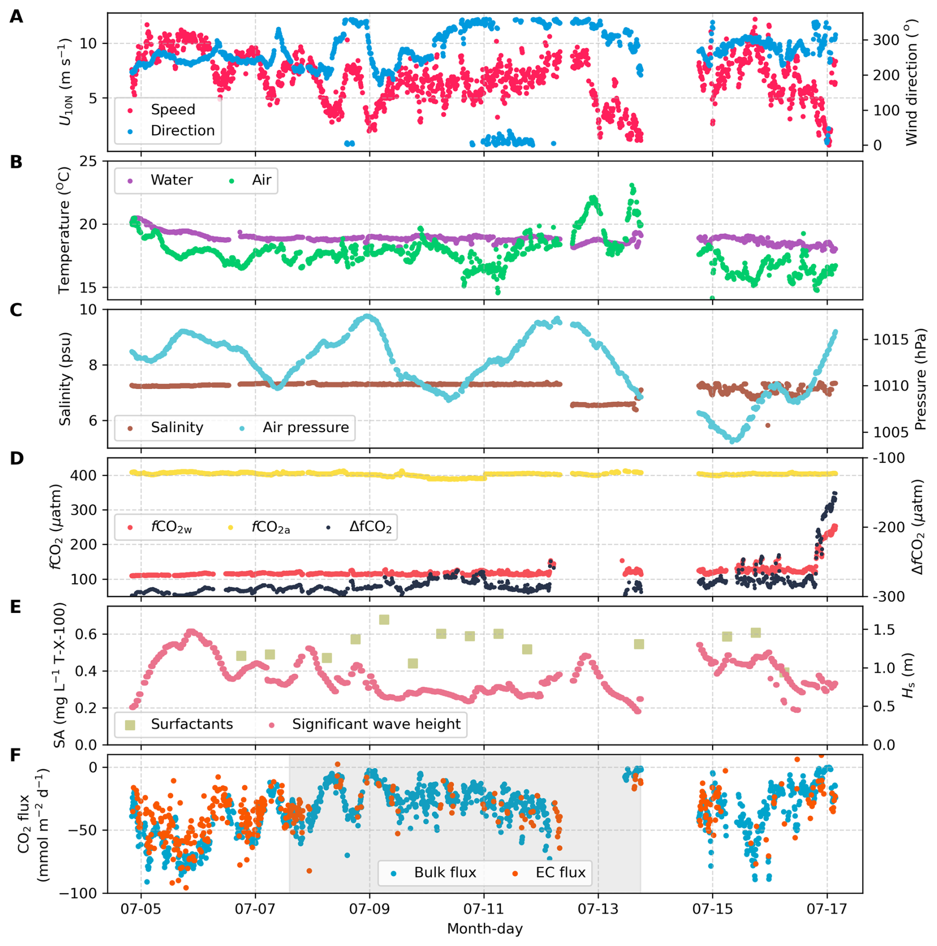
Figure 2 Ten min averages of environmental variables and air–sea CO₂ flux. (A) Neutral 10 m wind speed (U_10N, red) and wind direction (blue). (B) Surface seawater temperature (purple) and air temperature (green). (C) Seawater salinity (brown) and sea-level air pressure (light-blue). (D) CO₂ fugacity in surface seawater (red) and atmosphere (yellow), and their difference (ΔfCO₂, black). (E) Surface microlayer surfactant activity (SA, light green squares) and significant wave height extracted from ERA5 (H_s, red); (F) Bulk CO₂ flux estimates (blue, based on K₆₆₀ parameterisation from Ho et al., 2006) and EC CO₂ flux observations (orange). The dual-tracer tracing period is indicated by the light gray shading. Data are missing from 12–14 July due to a medical event and a temporary shortage of liquid nitrogen, which required the vessel to leave the primary study area.

3 Results

3.1 Environmental variables and the CO₂ flux

During CenBASE, winds predominantly originated from the west to north sector (Fig. 2A), with an effective fetch of approximately 50–300 km in the main study area (Fig. A1, Appendix). The wind speed ranged from 1 to 12 m s⁻¹ (Fig. 2A). Water depth across the central Baltic Sea study site ranged from ∼ 50 to 250 m. Surface water was generally warmer than the overlying air (Fig. 2B), resulting in an unstable boundary layer. Surface salinity remained consistent at approximately 7.3 throughout the study region (Fig. 2C). The cruise took place shortly after a summer phytoplankton bloom, resulting in remarkably low sea surface fCO₂ (∼ 120 µatm; Fig. 2D). Atmospheric fCO₂ remained constant at ∼ 403 µatm, creating a strong air–sea gradient (ΔfCO₂≈ −280 µatm on average; Fig. 2D) that generated strong ocean CO₂ uptake signals.

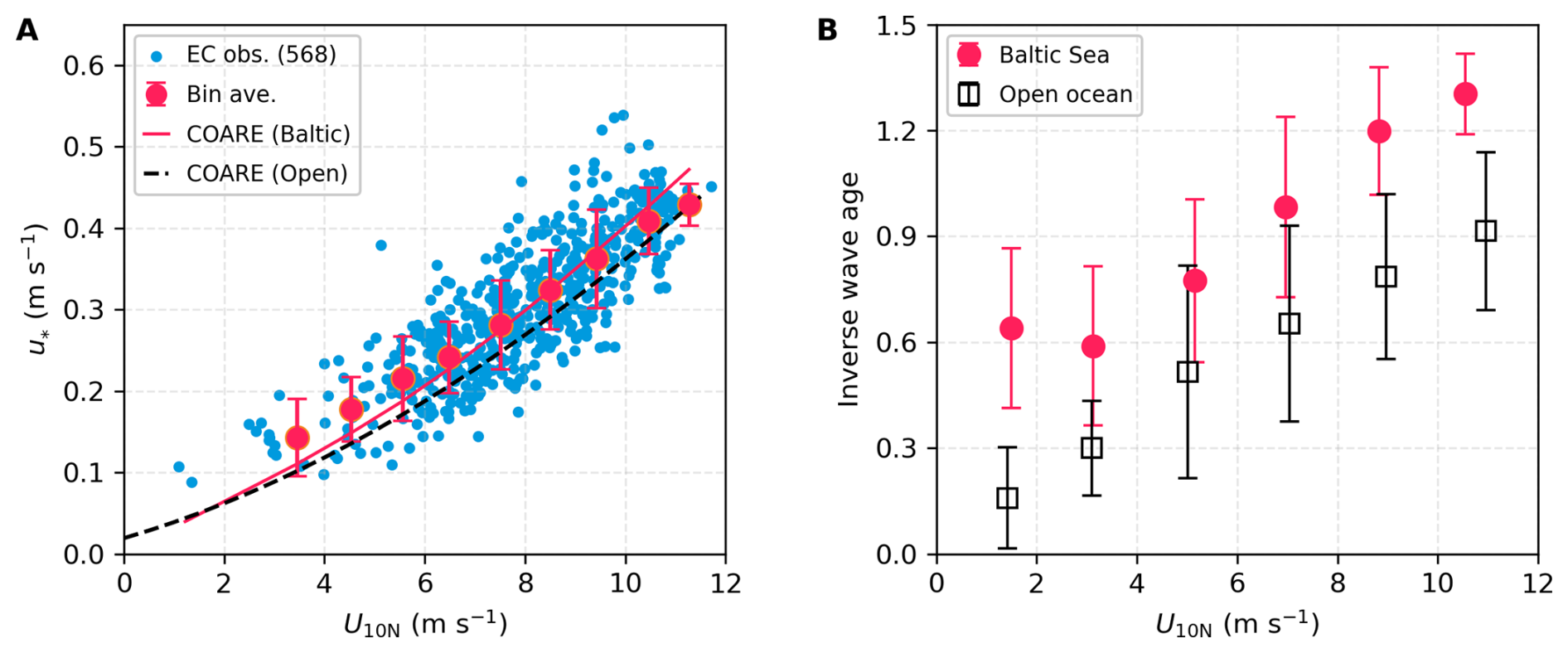
Figure 3 Friction velocity (u_∗) and inverse wave age in the Baltic Sea (CenBASE) and open ocean. (A) u_∗ derived from EC air–sea momentum fluxes versus 10 m neutral wind speed (U_10N). Blue dots: 10 min u_∗ observations during CenBASE (568 points), with red points corresponding to bin averages (per 1 m s⁻¹). Red line: u_∗ simulated by COARE3.6 using the Baltic Sea environmental data; Black-dashed line: COARE3.6 simulations in the open ocean. (B) Inverse wave age ($U_{\mathrm{10}\mathrm{N}}/C_p$) in the Baltic Sea (red dots) and open ocean (black squares). Error bars denote ± 1 standard deviation (SD) of bin averages. The hourly wave parameters are shown in Fig. A2 of the Appendix.

Surface microlayer surfactant activity (SA), expressed as Triton-X-100 equivalents, was relatively constant at 0.54 ± 0.08 mg L⁻¹ (Fig. 2E), significantly higher than typical open-ocean values (0.1–0.2 mg L⁻¹; Mustaffa et al., 2020; Sabbaghzadeh et al., 2017). Modeled significant wave height (H_s) remained below 1.5 m (Fig. 2E), lower than expected for comparable wind speeds in the open ocean (Fig. A2). Bulk CO₂ fluxes estimated from the measured ΔfCO₂ and an open-ocean dual-tracer K₆₆₀ parameterisation (Ho et al., 2006) were higher than observed EC fluxes under high wind speeds and lower than observed EC fluxes under low wind speeds (Figs. 2F and A3). During the tracer-tracking period (8–14 July), frequent ship heading changes reduced EC flux quality, leading to most valid EC measurements being obtained from outside this period (Fig. 2F, light-gray shading). Nevertheless, as both EC and dual-tracer were collected in the same study area, the K from both methods can be reasonably considered simultaneous measurements.

3.2 Friction velocity

The friction velocity is a key parameter characterizing near-surface turbulence. Observed values of u_∗ from EC momentum fluxes during CenBASE were 10 % higher than modelled open ocean u_∗ at the same wind speeds (Fig. 3A), likely reflecting fetch-related differences. The wave field in the central Baltic Sea is much younger than in the open ocean, with wave age ∼ 60 % lower at the same wind speed (Fig. 3B). The waves are shorter and steeper than in the open ocean (Fig. A2). This wave field enhances sea surface roughness and elevates u_∗ relative to the open sea. u_∗ predicted by the COARE3.6 model, when forced with observed environmental and extracted wave parameters during CenBASE, broadly agrees with measurements (Fig. 3A). This suggests that the COARE model remains applicable in fetch-limited marine environments when wave information is included, despite being developed primarily from open-ocean observations (Edson et al., 2013). Given that u_∗ is an indicator of surface wind-induced turbulence, this elevated u_∗ is expected to enhance CO₂ transfer velocity (see Sect. 3.4).

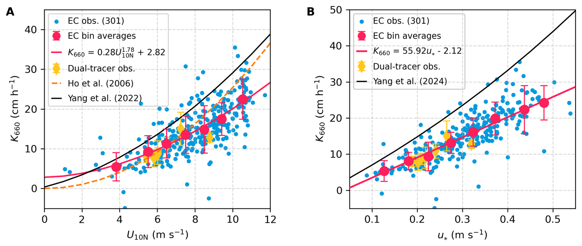
Figure 4 Gas transfer velocity ($K_{\mathrm{660}\mathit{\_}{\mathrm{CO}}_{\mathrm{2}}}$) in the central Baltic Sea during the CenBASE cruise. (A) Relationships between K₆₆₀ and U_10N. (B) Relationships between K₆₆₀ and observed u_∗. Blue dots in both panels represent 10 min $K_{\mathrm{660}\mathit{\_}{\mathrm{CO}}_{\mathrm{2}}}$ (N=301), with red dots denoting bin averages (1 m s⁻¹ U_10N bins or 0.05 m s⁻¹u_∗ bins) ± 1 SD. Red lines indicate the fit to the bins, with R² of 0.48 for the fit with U_10N and 0.59 for the fit with u_∗. Yellow diamonds show dual-tracer (DT) transfer velocities ($K_{\mathrm{660}\mathit{\_}{}^{\mathrm{3}}\mathrm{He}/{\mathrm{SF}}_{\mathrm{6}}}$) measured concurrently with EC. The orange line in panel (A) denotes the open ocean DT-based parameterisation from Ho et al. (2006). The black lines in panels (A) and (B) correspond to the open-ocean EC-based parameterisations of Yang et al. (2022; U_10N-dependent) and Yang et al. (2024; u_∗ and sea-state dependent), respectively.

3.3 Gas transfer velocities from EC and DT

The CO₂ transfer velocity ($K_{\mathrm{660}\mathit{\_}{\mathrm{CO}}_{\mathrm{2}}}$) was derived from EC air–sea CO₂ flux and ΔfCO₂ observations using Eq. (1). After quality control, 301 valid 10 min $K_{\mathrm{660}\mathit{\_}{\mathrm{CO}}_{\mathrm{2}}}$ data points were retained (Fig. 4). The large |ΔfCO₂| (∼ 280 µatm) ensured accurate $K_{\mathrm{660}\mathit{\_}{\mathrm{CO}}_{\mathrm{2}}}$ derivations, with hourly uncertainties of ∼ 20 % (Fig. A4), substantially lower than typical cruise-based uncertainties (e.g., ∼ 30 % during the HiWinGS cruise; Blomquist et al., 2017). The cool skin correction (reduces ΔfCO₂ by ∼ 2 µatm; Woolf et al., 2016) is negligible relative to the observed ΔfCO₂ and was therefore ignored. K₆₆₀ from the DT experiment is summarized in Appendix A1.

The EC dataset offers high temporal resolution (∼ 10 min), enabling investigation of small-scale processes influencing gas exchange. The EC observations span a broad range of wind speeds (1 to 12 m s⁻¹, Fig. 4A), providing a robust constraint of $K_{\mathrm{660}\mathit{\_}{\mathrm{CO}}_{\mathrm{2}}}$ under low-to-moderate wind conditions. In contrast, DT-derived K₆₆₀ represents daily averages, in which short-term extremes (i.e., low and high wind conditions) are smoothed, resulting in seven observations concentrated at U_10N of 5–9 m s⁻¹ (Fig. 4A). Within this wind range, DT-and EC-derived K₆₆₀ values are in good agreement, with the former on average being only slightly (∼ 8 %) lower than the latter (Fig. 4).

DT-derived K₆₆₀ values during CenBASE also generally agree with the open-ocean DT-based parameterisation of Ho et al. (2006) under equivalent wind speeds (orange dashed line in Fig. 4A), with the former on average being only ∼ 7 % lower than the latter. However, EC-derived $K_{\mathrm{660}\mathit{\_}{\mathrm{CO}}_{\mathrm{2}}}$ values deviate systematically from this open-ocean relationship (Ho et al., 2006), being higher at low wind speeds (1–7 m s⁻¹, +12 %) and lower at high wind speeds (7–12 m s⁻¹, −18 %) (Fig. 4A). This divergence does not contradict the agreement between the DT-and EC-based K₆₆₀ observations, as this agreement falls within the 5–9 m s⁻¹ range (where the DT data concentrate). Fitting $K_{\mathrm{660}\mathit{\_}{\mathrm{CO}}_{\mathrm{2}}}$ with U_10N reveals a weaker wind speed dependence than the open ocean DT-based parameterisation (Fig. 4A). It is worth noting that including a constant term in the $K_{\mathrm{660}\mathit{\_}{\mathrm{CO}}_{\mathrm{2}}}$-U_10N fitting function (i.e., $K_{\mathrm{660}\mathit{\_}{\mathrm{CO}}_{\mathrm{2}}}=a{U}_{\mathrm{10}\mathrm{N}}^{\mathrm{b}}+c$, R² = 0.48) improves the fit compared to a purely power-law form (i.e., $K_{\mathrm{660}\mathit{\_}{\mathrm{CO}}_{\mathrm{2}}}=a{U}_{\mathrm{10}\mathrm{N}}^{\mathrm{b}}$, R² = 0.42) (Fig. A5), suggesting a non-zero CO₂ exchange (∼ 3 cm h⁻¹) under calm conditions. This is unsurprising, since the chemical enhancement (Cole and Caraco, 1998; Fairall et al., 2022; Yang et al., 2022) and likely buoyancy flux sustain CO₂ transfer at low wind speeds (McGillis et al., 2004; Wanninkhof et al., 2009).

Notably, the DT data collected during CenBASE provide only limited constraints at wind speeds below 5 m s⁻¹ and above 9 m s⁻¹, and the K₆₆₀-U_10N relationship derived from these data is sensitive to the chosen functional form (Fig. A5). Moreover, the DT-based open-ocean K₆₆₀ estimates are lower than the EC CO₂-based estimates across the wind speed range observed during CenBASE (Fig. 4A), likely reflecting differences in methodology. Because the CenBASE DT data are interpreted elsewhere (Dobashi et al., 2026), and, more importantly, because the EC measurements resolve finer-scale processes and ensure methodological consistency, the subsequent section focuses on comparing EC CO₂ observations in the Baltic Sea with those in the open ocean.

3.4 Suppression of air–sea CO₂ exchange

The EC-derived $K_{\mathrm{660}\mathit{\_}{\mathrm{CO}}_{\mathrm{2}}}$ during CenBASE was generally lower than open-ocean EC CO₂ transfer velocities (Yang et al., 2022; 2024) (Fig. 4A and B), indicating a substantial suppression of CO₂ exchange in the Baltic Sea. To explain this reduction, we partition the total gas transfer velocity (K₆₆₀) into interfacial (K_i660) and bubble-mediated (K_b660) components (i.e., $K_{\mathrm{660}}=K_{\mathrm{i}\mathrm{660}}+K_{\mathrm{b}\mathrm{660}}$). K_i660 is primarily driven by wind stress or u_∗, whereas K_b depends on both the wind forcing and sea state. A machine-learning analysis of 15 open ocean datasets identified significant wave height (H_s, including both windsea and swell) as a key proxy for sea state that strongly affects $K_{\mathrm{660}\mathit{\_}{\mathrm{CO}}_{\mathrm{2}}}$ (Yang et al., 2024). Based on this analysis, Yang et al. (2024) express the K₆₆₀ as (Fig. 4B, black line):

$$\begin{array}{}\text{(3)}& K_{\mathrm{660}}=K_{\mathrm{i}\mathrm{660}}+K_{\mathrm{b}\mathrm{660}}=\mathrm{55}{u}_{\ast }+\mathrm{10}{u}_{\ast }{H}_{\mathrm{s}}\end{array}$$

Because K_b depends on solubility, normalizing it using the Schmidt number (i.e., converting K_b to K_b660) may not be strictly appropriate. However, the sensitivities of the CO₂ transfer velocity to ${\mathit{Sc}}^{-\mathrm{1}/\mathrm{2}}$ and α⁻¹ are nearly identical (see Fig. A1 in Dong et al., 2025). Therefore, normalization using either Sc or α produces almost the same gas transfer velocities. For simplicity and consistency, we adopt the ${\mathit{Sc}}^{-\mathrm{1}/\mathrm{2}}$-based normalization in this study.

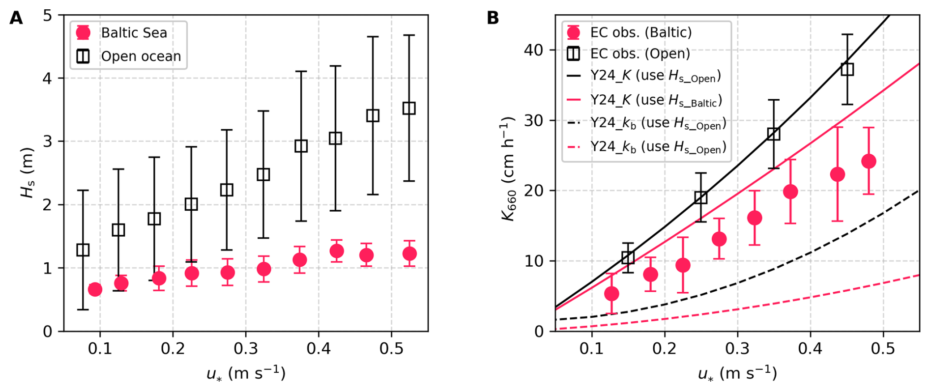
Figure 5 Comparison of significant wave height (H_s) and $K_{\mathrm{660}\mathit{\_}{\mathrm{CO}}_{\mathrm{2}}}$ between the Baltic Sea and the open ocean. (A) H_s in the Baltic Sea during CenBASE (red dots) and in the open ocean (black squares), with error bars representing ± 1 SD. The data are extracted from ERA5 according to the EC cruise tracks (Yang et al., 2022) and the CenBASE cruise track. (B) $K_{\mathrm{660}\mathit{\_}{\mathrm{CO}}_{\mathrm{2}}}$ observations in the Baltic Sea during CenBASE (red dots, the same as the red dots in Fig. 4B) and in the open ocean (black squares, Yang et al., 2022). The black and red solid lines correspond to the parameterised total CO₂ transfer velocity (i.e., $K_{\mathrm{660}\mathit{\_}{\mathrm{CO}}_{\mathrm{2}}}$ from Eq. 3; Yang et al., 2024) using the open ocean and the Baltic Sea H_s, respectively. The black and red dashed lines denote the parameterised bubble-mediated transfer component (K_b660; Eq. 3) using the open ocean and the Baltic Sea H_s, respectively.

Table 1 Comparison of mean gas transfer velocities between measurements in the Baltic Sea and estimates using the open ocean parameterisation from Yang et al. (2024) under identical wind speed conditions (Eq. 3). The percentages in parentheses in the K_i, K_b, and K columns indicate the relative difference between the Baltic Sea and the open ocean. The last column is the uncertainty assessment of the values in the K column with the values in parentheses representing the relative uncertainties. The positive (negative) sign represents the enhancement (suppression).

The observed EC K₆₆₀ during CenBASE averaged 14.9 cm h⁻¹. To compare this value with open-ocean conditions at equivalent wind speeds, we apply the wind-speed observations from the CenBASE cruise (i.e., wind speed values shown in Fig. 4A) to Eq. (3) to estimate open-ocean K₆₆₀, yielding average values of K_i660 = 15.1 cm h⁻¹, K_b660 = 7.0 cm h⁻¹, and K₆₆₀ = 22.1 cm h⁻¹. This means that the observed K₆₆₀ during CenBASE was 33 % (7.2 cm h⁻¹) lower than the open-ocean K₆₆₀ estimate.

Equation (3) implies a linear dependence of $K_{\mathrm{660}\mathit{\_}{\mathrm{CO}}_{\mathrm{2}}}$ on u_∗. Regression of the observed $K_{\mathrm{660}\mathit{\_}{\mathrm{CO}}_{\mathrm{2}}}$ against u_∗ indeed yields an approximately linear relationship (Fig. 4B), consistent with prior findings at low-to-moderate winds (Landwehr et al., 2018; Yang et al., 2022). Additionally, the $K_{\mathrm{660}\mathit{\_}{\mathrm{CO}}_{\mathrm{2}}}$-u_∗ fit (R² = 0.59) outperforms the $K_{\mathrm{660}\mathit{\_}{\mathrm{CO}}_{\mathrm{2}}}$-U_10N fit (R² = 0.48), confirming that u_∗ better captures variability in gas transfer velocity than U_10N (Jähne et al., 1987; Landwehr et al., 2018; Yang et al., 2022). As shown in Fig. 3A, the observed u_∗ during CenBASE was ∼ 10 % higher than open-ocean values under equivalent wind speeds, implying a ∼ 10 % enhancement in $K_{\mathrm{660}\mathit{\_}{\mathrm{CO}}_{\mathrm{2}}}$ due to fetch-related increases in shear stress (Vickers and Mahrt, 1997). It is important to note that the observed 33 % reduction in $K_{\mathrm{660}\mathit{\_}{\mathrm{CO}}_{\mathrm{2}}}$ includes this enhancement, suggesting that CO₂ exchange was suppressed even more, by ∼ 43 % (9.2 cm h⁻¹) relative to open-ocean conditions.

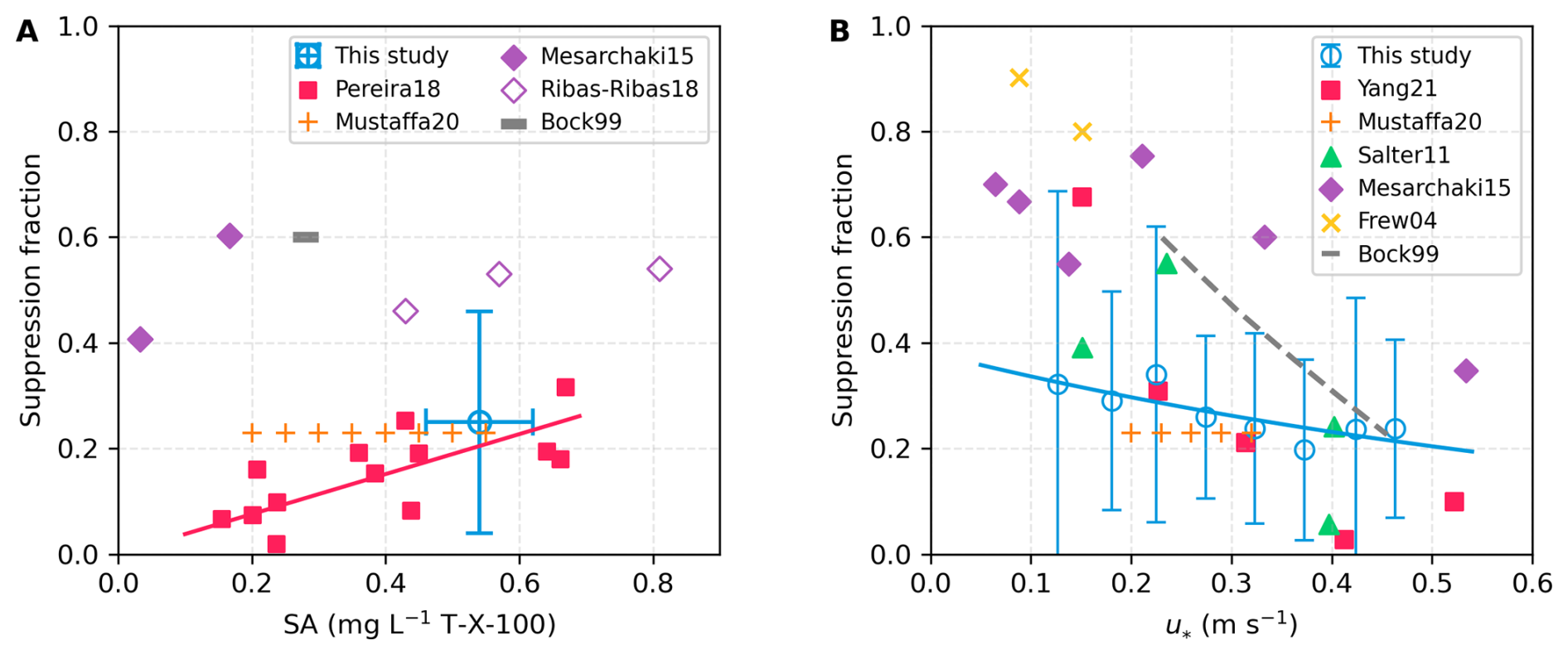
Figure 6 Surfactant-induced suppression fraction on K₆₆₀ (sf) from this study and previous work. (A) sf as a function of surfactant concentration under low-moderate wind speeds. The blue circle shows the mean constrained sf from this study; horizontal and vertical error bars denote the standard deviation of observed SA and the associated uncertainty of the constrained sf. Red squares indicate sf from wave-tank experiments with natural Atlantic seawater at wind speeds < 13 m s⁻¹ (Pereira et al., 2018), with the red line showing the linear fit (sf = 38 × SA). Orange pluses show sf constrained from field K₆₆₀ observations using the chamber technique with natural surfactant (Mustaffa et al., 2020). Diamonds (filled/unfilled) and the grey dash represent wave-tank studies using artificial soluble surfactants (Mesarchaki et al., 2015; Ribas-Ribas et al., 2018; Bock et al., 1999). (B) sf as a function of u_∗. Blue circles show sf constrained from the residual suppression of observed $K_{\mathrm{660}\mathit{\_}{\mathrm{CO}}_{\mathrm{2}}}$ from this study, with error bars indicating uncertainties. The blue line corresponds to the fit based on the blue circles (0.38 × e^1.25u∗, R² = 0.65). Red squares represent values derived from an EC-based CO₂ transfer velocity study (Yang et al., 2021). Orange pluses denote the Mustaffa et al. (2020) dataset with surfactant concentrations of 0.2–0.6 mg L⁻¹. Green triangles show sf inferred from EC-based DMS and DT exchange experiments in artificial insoluble surfactant patches (Salter et al., 2011). Purple diamonds represent Mesarchaki et al. (2015), who used ∼ 0.2 mg L⁻¹ of artificial soluble surfactant. Yellow crosses indicate sf derived from coastal heat transfer measurements (Frew et al., 2004). The grey dashed line shows laboratory experiments with artificial soluble surfactants at ∼ 0.3 mg L⁻¹ (Bock et al., 1999).

According to Eq. (3), K_b is linearly dependent on H_s. Due to the limited fetch, the H_s during CenBASE was 57 % lower than in the open ocean at the equivalent u_∗ (Fig. 5A, Table 1), and this reduction is expected to cause a comparable decrease in K_b. Using the extracted H_s values from ERA5 for CenBASE, the parameterised K_b660 decreases on average from 7.0 to 4.0 cm h⁻¹, corresponding to an 18 % suppression on the total $K_{\mathrm{660}\mathit{\_}{\mathrm{CO}}_{\mathrm{2}}}$ (Fig. 5B; Table 1), explaining about half of the observed suppression during CenBASE.

Surfactants inhibit both interfacial (e.g., Frew, 1997) and bubble-mediated gas exchange (e.g., Woolf, 1993), and their concentrations in the Baltic Sea are substantially higher than in the open ocean. We assume that all residual suppression of $K_{\mathrm{660}\mathit{\_}{\mathrm{CO}}_{\mathrm{2}}}$ during CenBASE, which cannot be explained by fetch effects, is caused by surfactants. Under this assumption, the residual 25 % suppression (i.e., 5.4 cm h⁻¹; Fig. 5B and Table 1) reflects the impact of elevated surfactant levels. This effect is not captured by the Yang et al. (2024) parameterisation, which is based primarily on open-ocean observations characterized by low surfactant concentrations (Wurl et al., 2011; Fig. A6).

The resulting suppression fraction (sf) is consistent in magnitude with previous field-based estimates (Fig. 6; Mustaffa et al., 2020; Salter et al., 2011; Yang et al., 2021) within uncertainty (see Sect. 3.5). The constrained sf is generally smaller than laboratory-derived values (Fig. 6A), likely due to challenges in extrapolating laboratory conditions to the field. Notably, previous studies report conflicting relationships between sf and surfactant concentration. Some show increasing sf with increasing concentration (Mesarchaki et al., 2015; Pereira et al., 2018; Ribas-Ribas et al., 2018), whereas others identify a threshold concentration above which sf shows little change (Mustaffa et al., 2020; Schmidt and Schneider, 2011) (Fig. 6A). Because surfactant concentrations were nearly constant during CenBASE, we cannot assess this relationship here.

Several studies also show that sf decreases with wind speed (Fig. 6B; Bock et al., 1999; Mesarchaki et al., 2015; Salter et al., 2011; Yang et al., 2021), and the sf constrained here aligns well with these findings, especially those from field observations. Fitting sf as a function of u_∗ yields a correction factor (i.e., 1−sf) that can be applied to Eq. (3) to account for surfactant effects, generating the updated parameterisation:

$$\begin{array}{}\text{(4)}& K_{\mathrm{660}}=(\mathrm{1}-\mathrm{0.38}{e}^{-\mathrm{1.25}{u}_{\ast }})(\mathrm{55}{u}_{\ast }+\mathrm{10}{u}_{\ast }{H}_{\mathrm{s}})\end{array}$$

This parameterisation reflects conditions during CenBASE, where the surfactant concentration was relatively stable at ∼ 0.5 mg L⁻¹. If a SA concentration-dependent sf is needed, one option is the published linear relationship $\mathrm{sf}=\mathrm{0.32}\mathrm{SA}+\mathrm{0.025}$ (Pereira et al., 2018). However, this formulation maybe physically inconsistent because it predicts a non-zero suppression even when SA=0, whereas sf should theoretically approach zero in surfactant-free conditions. To address this, we re-evaluated the same dataset used in the original study (Pereira et al., 2018) and fitted a proportional relationship that passes through the origin: sf=0.38SA. The goodness-of-fit (R² = 0.49) is only marginally lower than the original relationship (0.51, Pereira et al., 2018), indicating that the proportional form captures the data nearly as well while remaining physically realistic. For the mean CenBASE surfactant concentration (SA = 0.54 mg L⁻¹), this relationship yields sf = 0.21. Applying this SA-dependent suppression to the wind-dependent correction in Eq. (4) results in the combined parameterisation:

$$\begin{array}{}\text{(5)}& K_{\mathrm{660}}={\displaystyle \frac{\mathrm{1}-\mathrm{0.38}\mathrm{SA}}{\mathrm{0.79}}}(\mathrm{1}-\mathrm{0.38}{e}^{-\mathrm{1.25}{u}_{\ast }})(\mathrm{55}{u}_{\ast }+\mathrm{10}{u}_{\ast }{H}_{\mathrm{s}})\end{array}$$

Previous studies have suggested that water-side convection may influence gas exchange in both open-ocean (McGillis et al., 2004) and Baltic conditions (Rutgersson and Smedman, 2010). During CenBASE, a small spar buoy recorded oxygen, temperature, and salinity at depths of 1.2 and 2.9 m. Dissolved oxygen exhibited small-scale variability with similar patterns at both depths (Fig. A7), indicating coherent near-surface structure over 5–20 m scales, likely driven by wind-induced turbulence intermittently exposing surface patches to the atmosphere. In contrast, no corresponding variability was observed in temperature or salinity (Fig. A7), suggesting that convection played a negligible role in gas exchange under the observed conditions. This supports our assumption that the deviation in $K_{\mathrm{660}\mathit{\_}{\mathrm{CO}}_{\mathrm{2}}}$ between the Baltic Sea and the open ocean can be fully attributed to the combined effects of limited fetch and elevated surfactant levels.

3.5 Uncertainty analysis

The quantification results shown above are not free from uncertainty. First, we use the $K_{\mathrm{b}}\propto u_{\ast }{H}_{\mathrm{s}}$ relationship for the bubble component, which fits best with the EC-based $K_{\mathrm{660}\mathit{\_}{\mathrm{CO}}_{\mathrm{2}}}$ observations (Yang et al., 2024). However, alternative formulations have been proposed, such as $K_{\mathrm{b}}\propto u_{\ast }^{\mathrm{1.67}}{H}_{\mathrm{s}}^{\mathrm{0.67}}$ (Deike and Melville, 2018) and $K_{\mathrm{b}}\propto u_{\ast }^{\mathrm{0.9}}{H}_{\mathrm{s}}^{\mathrm{0.9}}$ (Brumer et al., 2017a; Fairall et al., 2022). These different exponents indicate that the relative contributions of u_∗ and H_s to gas exchange may vary slightly, introducing parameterisation uncertainty. Yang et al. (2024) reported that the R² for the fit (i.e., Eq. 3) is ∼ 0.75, indicating that ∼ 25 % of the variance in the observed K remains unexplained by the parameterisation. We therefore assign a 25 % uncertainty to the parameterisation given in Eq. (3). This uncertainty propagates through the suppression estimates. For instance, the uncertainty in the u_∗-related K enhancement estimate is approximately 0.6 cm h⁻¹ (i.e., 2.2 cm h⁻¹ × 25 %). The suppression analysis uses H_s data derived from ERA5 reanalysis, which likely carries an uncertainty of about 30 % in the Baltic Sea (Giudici et al., 2023). Consequently, the uncertainty in the H_s-related suppression estimate is ∼ 1.6 cm h⁻¹ (i.e., $\sqrt{(\mathrm{4.0}\times \mathrm{25}\mathit{\%}{)}^{\mathrm{2}}+(\mathrm{4.0}\times \mathrm{30}\mathit{\%}{)}^{\mathrm{2}}}$ cm h⁻¹). The uncertainty associated with the surfactant-related suppression is substantially larger because it is not directly determined but inferred as a residual after accounting for other components. Combining the propagated uncertainties from the parameterised total K and from two fetch-induced suppression estimates yields an uncertainty of 5.8 cm h⁻¹ (i.e., $\sqrt{(\mathrm{22.1}\times \mathrm{25}\mathit{\%}{)}^{\mathrm{2}}+{\mathrm{0.6}}^{\mathrm{2}}+{\mathrm{1.6}}^{\mathrm{2}}}$ cm h⁻¹), corresponding to approximately 110 % of the estimated suppression value (Table 1).

Furthermore, it is worth noting that the two corrections in Eq. (5) (i.e., the SA-sf correction and the u_∗-SA correction) are implicitly assumed to be independent. However, potential interactions between u_∗-dependent SA variation and the SA influence on sf may introduce additional uncertainty into Eq. (5).

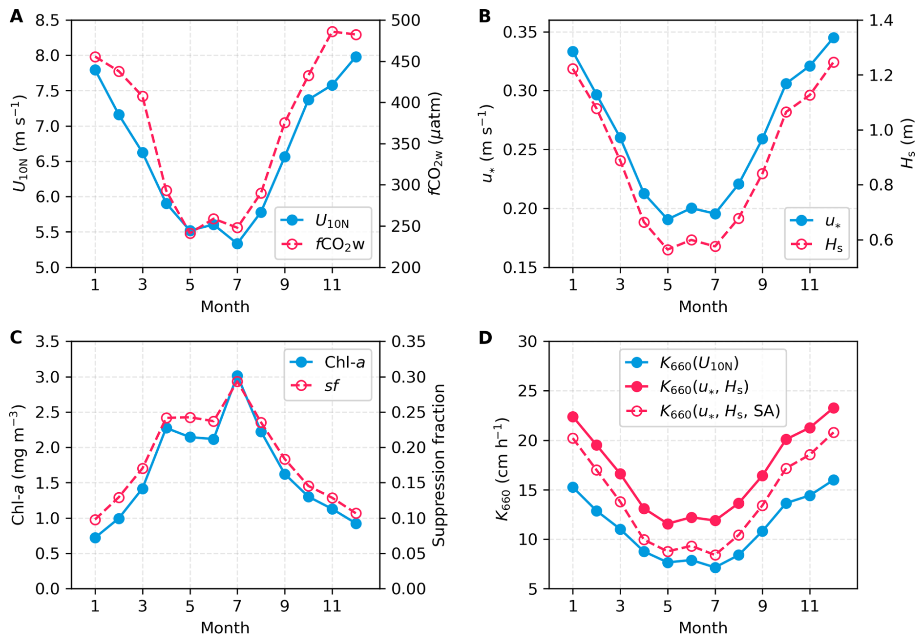
Figure 7 Climatological seasonal variations of environmental variables and gas transfer velocities in the Baltic Sea. (A) U_10N (blue) and fCO_2w (red; Bittig et al., 2024). (B) u_∗ (blue) and H_s (red). U_10N, u_∗, and H_s are averaged from the ERA5 monthly reanalysis data product (Hersbach et al., 2020) for 1998–2018. (C) Surfactant concentrations scaled from monthly chlorophyll a (Chl a) (Pitarch et al., 2016) and surfactant-induced suppression fraction of K₆₆₀ based on the SA- and U₁₀-dependent parameterisation (Eq. 5). (D) K₆₆₀ estimated from different parameterisations: U_10N-based (blue; Ho et al., 2006), u_∗-H_s-based (red solid; Eq. 3, Yang et al., 2024); u_∗-H_s-SA-based (red dashed; Eq. 5).

3.6 Implications for Baltic Sea CO₂ flux estimates

The CenBASE cruise took place during the summer bloom (July), when chlorophyll a (Chl a) is high (Pitarch et al., 2016) and fCO_2w is strongly reduced by primary productivity (e.g., Parard et al., 2016; Bittig et al., 2024). To upscale these results, we adopt a fCO_2w product from Bittig et al. (2024) to examine how fetch and surfactants shape the climatological CO₂ flux of the Baltic Sea. This climatological fCO_2w product is derived by combining observations and model patterns. The fCO_2w indicates a CO₂ sink in summer and a source in winter (Fig. 7A). However, weaker summer winds and stronger winter winds suggest that the magnitudes of uptake and outgassing may be similar. Seasonal cycles of u_∗ and H_s closely follow wind speed (Fig. 7B), while Chl a peaks during the spring-summer bloom and remains low in winter (Fig. 7C). We estimate monthly surfactant concentrations by scaling the July CenBASE value (0.54 mg L⁻¹) with monthly Chl a concentrations following the idea of Wurl et al. (2011) and using the formula 0.54 × Chl a/Chl a_July mg L⁻¹. Equation (5) is then used to compute the corresponding suppression of gas transfer, $\mathrm{1}-\frac{\mathrm{1}-\mathrm{0.38}\mathrm{SA}}{\mathrm{0.79}}(\mathrm{1}-\mathrm{0.38}{e}^{-\mathrm{1.25}{u}_{\ast }}$). The resulting sf reflects the seasonal Chl a cycle and modulations by u_∗, yielding ∼ 25 % suppression in summer and ∼ 10 % in winter (Fig. 7C). However, surfactant concentrations are not solely determined by Chl a; for example, humic acids also act as surfactants (e.g., Klavins and Purmalis, 2010), and the Baltic Sea is known for elevated humic acid levels due to significant terrestrial inputs (Hammer et al., 2017). Therefore, estimating surfactant levels solely from Chl a has inherent limitations.

We estimate K₆₆₀ using three parameterisation schemes: the conventional open ocean DT-based U_10N formulation (Ho et al., 2006), the open ocean EC CO₂-based u_∗-H_s formulation (Eq. 3; Yang et al., 2024), and the Baltic Sea EC CO₂-based u_∗-H_s-SA formulation (Eq. 5). Although all these schemes reproduce similar seasonal patterns, their magnitudes differ (Fig. 7D), reflecting sea state and surfactant effects as well as methodological differences. The u_∗-H_s-SA parameterisation yields lower values than the u_∗-H_s scheme because it incorporates surfactant-induced suppression from the surfactant. This suppression is especially strong in summer when SA concentrations are highest, leading to the largest discrepancies between the estimated climatological K₆₆₀ from the u_∗-H_s-SA and the u_∗-H_s schemes. As shown in Sect. 3.4, K₆₆₀ during CenBASE has been reduced by 33 %. Notably, this reduction is relative to open-ocean EC-based estimates. However, compared with the open ocean DT-based U_10N formulation, however, this reduction occurs only at wind speeds above ∼ 7 m s⁻¹. At lower wind speeds, the EC-based K₆₆₀ observations during CenBASE exceed the DT-based estimates (Fig. 4A). Because climatological Baltic Sea wind speeds are typically below 7 m s⁻¹ in Spring, Summer, and Autumn (Fig. 7A), the u_∗-H_s-SA parameterisation produces higher K₆₆₀ than the U_10N formulation in these seasons. In winter, despite higher wind speeds, the u_∗-H_s-SA scheme still exceeds the U_10N-based estimates due to modulation of the surfactants. The SA concentration in winter is estimated to be three times lower than during the summer CenBASE cruise (Fig. 7C), resulting in much weaker suppression.

Overall, relative to the conventional U_10N formulation (Ho et al., 2006), the u_∗-H_s-SA parameterisation increases K₆₆₀ in all seasons, enhancing both summer CO₂ uptake by ∼ 10 % and winter outgassing by ∼ 30 %, and amplifying the seasonal cycle by ∼ 40 %. These opposing seasonal effects are expected to largely compensate, resulting in only a modest change in the annual mean CO₂ flux.

4 Discussion and conclusions

A robust understanding of air–sea gas exchange mechanisms is fundamental for accurately quantifying CO₂ fluxes, which is essential for accurate carbon budgets and climate projections. Most previous studies have focused on the open ocean, where K₆₆₀ is typically parameterised as a function of wind speed. In contrast, marginal seas such as the Baltic Sea exhibit more complex dynamics due to limited fetch and abundant surfactants, which modulate the wind speed dependence of gas exchange. To investigate these processes, a dedicated experiment was conducted in the central Baltic Sea during the CenBASE cruise, employing two commonly used techniques: eddy covariance and dual-tracer methods. The K₆₆₀ derived from both techniques agrees well, confirming the reliability of both methods for gas transfer velocity observations. The observed CO₂ transfer velocity shows a significant reduction compared to the open-ocean CO₂ observations and parameterisations under comparable wind conditions (Yang et al., 2024; Fig. 4). This reduction can be attributed to three competing processes (summarized in Fig. 8): (1) a 10 % enhancement from fetch-limited increases in friction velocity, (2) an 18 % suppression from reduced significant wave height, and (3) a 25 % suppression from elevated surfactant concentrations. Together, these effects explain the overall 33 % reduction in CO₂ exchange during CenBASE relative to the EC-based open ocean $K_{\mathrm{660}\mathit{\_}{\mathrm{CO}}_{\mathrm{2}}}$.

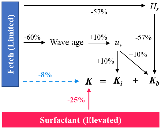
Figure 8 Schematic illustrating how fetch and surfactants modulate the CO₂ transfer velocity (K) in the Baltic Sea relative to the open ocean. Values denote the relative magnitude of enhancement (+) or suppression (−) for each process (Table 1). Black arrows and their associated values indicate the effect of fetch on individual gas exchange components, while the blue value on the dashed arrow shows the net fetch effect on total K. The red value and arrow represent the constrained surfactant-induced suppression of K.

During CenBASE, fetch lengths ranged from 50–300 km, in contrast to more than 1000 km in the open ocean. The limited fetch exerts both enhancing and suppressing effects on gas exchange in the Baltic Sea (Fig. 8). Shorter fetch produces a younger wave field dominated by shorter and steeper waves, increasing surface roughness and thereby enhancing u_∗ and K₆₆₀. At the same time, limited fetch constrains wave development, leading to a ∼ 60 % reduction in H_s (Fig. 5A). As a key proxy for wave-breaking intensity (Brumer et al., 2017b; Deike, 2021; Zhao et al., 2003), reduction in H_s diminishes wave breaking and consequently suppresses bubble-mediated gas transfer (Dobashi and Ho, 2023; Fairall et al., 2006; Ocampo-Torres and Donelan, 1995; Woolf, 2005). These findings emphasize the need to incorporate sea-state dependence into K₆₆₀ parameterisations (Brumer et al., 2017a; Deike and Melville, 2018; Fairall et al., 2022; Yang et al., 2024). When direct wave observations are unavailable, reanalysis products (e.g., ERA5; Hersbach et al., 2020) can serve as a first-order estimate of wave conditions for K evaluation (Bessonova et al., 2025; Giudici et al., 2023).

Although bubble effects are expected to be stronger for low-solubility tracers such as ³He and SF₆ than for CO₂, the EC CO₂-derived and dual-tracer-derived K₆₆₀ values agreed closely (Fig. 4A). This is primarily because the bubble contribution to the total gas exchange during CenBASE was relatively small due to the low wind regime (Fig. 5B). According to the widely used model (Woolf, 1997), bubble-mediated transfer contributes ∼ 25 % to total CO₂ exchange and ∼ 35 % to ${}^{\mathrm{3}}\mathrm{He}/{\mathrm{SF}}_{\mathrm{6}}$ exchange under wind speeds of 0–12 m s⁻¹. This difference corresponds to only ∼ 1.5 cm h⁻¹ higher K₆₆₀ for dual tracers, which lies well within the measurement uncertainty and is therefore not practically distinguishable. Moreover, the much lower salinity in the Baltic Sea further limits the bubble-induced solubility dependence of K. Although the bubble size observations with the bubble cameras on a spar buoy did not work during CenBASE, it is well established that bubbles coalesce easily in fresh water (this is inhibited in salt water), so the initial bubble size distribution in fresher water quickly evolves towards larger bubbles through coalescence (e.g., De Leeuw et al., 2011). This coalescence effect has little influence on the gas transfer of moderately soluble gases such as CO₂ but reduces K_b for very low-solubility gases (e.g., ³He and SF₆) due to the reduction of bubble surface area, thereby narrowing the difference in K_b660 between CO₂ and ${}^{\mathrm{3}}\mathrm{He}/{\mathrm{SF}}_{\mathrm{6}}$. This also indicates that the parameterisation of the bubble-mediated component derived from open-ocean EC data (Yang et al., 2024) remains applicable to the Baltic Sea, despite differences in salinity and, thereby, the bubble-size distribution.

The suppression of gas exchange by surfactants has been well documented in laboratory studies, which report 10 %–65 % reductions in K depending on surfactant concentration (Bock et al., 1999; Frew et al., 1990; Goldman et al., 1988; Mesarchaki et al., 2015; Pereira et al., 2016, 2018; Ribas-Ribas et al., 2018; Schmidt and Schneider, 2011). Based on the empirical relationship derived by Pereira et al. (2018) using laboratory data, the CenBASE microlayer surfactant concentration (0.54 ± 0.08 mg L⁻¹) corresponds to an estimated ∼ 20 % reduction in K. Field studies have reported similar magnitudes of suppression (24 %–55 %) under artificial surfactant additions (Brockmann et al., 1982; Salter et al., 2011). More recently, field chamber measurements indicate ∼ 23 % suppression for natural surfactant levels exceeding 0.2 mg L⁻¹ (Mustaffa et al., 2020), and EC-based $K_{\mathrm{660}\mathit{\_}{\mathrm{CO}}_{\mathrm{2}}}$ observations have shown ∼ 30 % suppression at moderate winds (∼ 7 m s⁻¹) under likely high surfactant conditions (Yang et al., 2021). Thus, the 25 % suppression estimated in this study agrees well with previous laboratory and field results.

Our findings refine the mechanistic understanding of air–sea gas exchange and have important implications for estimates of coastal CO₂ flux estimates. Using the u_∗-H_s-SA parameterisation, both summer uptake and winter outgassing of CO₂ in the Baltic Sea increase compared to a conventional U_10N-based parameterisation, amplifying the seasonal cycle. Because many coastal regions exhibit similarly short fetches and elevated surfactant concentrations (Fig. A6), the mechanism-based parameterisation proposed here is expected to yield systematically different gas exchange efficiencies than conventional wind-speed-based formulations. The mechanism-based K parameterisation could alter coastal CO₂ flux estimates (e.g., Resplandy et al., 2024), influencing annual means, long-term trends, seasonal cycles, and spatial patterns. An improved estimate of the ocean CO₂ sink may also help reduce discrepancies between the data-based and model-based global carbon budgets (Friedlingstein et al., 2025). The improvement in the estimate of K is especially important for mCDR studies, which are often tested or developed in coastal environments (e.g., Ho et al., 2023). Beyond CO₂, the updated parameterisation may also apply to other greenhouse gases, such as N₂O, which share the same interfacial exchange mechanism and exhibit similar bubble-mediated behavior due to their comparable solubility. Application to DMS is also possible, provided the bubble-mediated component is omitted.

Despite the advances from the CenBASE campaign, several uncertainties remain. The surfactant-induced suppression was inferred from residual differences between Baltic Sea and open-ocean $K_{\mathrm{660}\mathit{\_}{\mathrm{CO}}_{\mathrm{2}}}$ after correcting for fetch effects, and therefore carries considerable uncertainty even though the magnitude is consistent with previous field constraints. We were unable to partition the surfactant-induced suppression between interfacial and bubble-mediated pathways because available evidence is insufficient to quantify their relative roles. Observations were limited to low-to-moderate wind speeds (< 12 m s⁻¹), preventing evaluation of the surfactant effect under high wind-speed conditions. Furthermore, surfactant concentrations were relatively uniform during CenBASE, so suppression could not be assessed across natural SA concentration gradients. Given the strong seasonal and spatial variability in biological production, the transferability of our quantified suppression values beyond the CenBASE conditions is uncertain. Addressing these limitations will require coordinated, multi-season observations across diverse fetch conditions, surfactant regimes, and wind speeds. Such efforts are essential for building a generalizable framework for gas exchange in marginal seas and for improving both regional CO₂ budgets and assessment of emerging mCDR applications.

Appendix A

A1 Dual-tracer experiments

The K was determined using the ${}^{\mathrm{3}}\mathrm{He}/{\mathrm{SF}}_{\mathrm{6}}$ dual tracer technique in addition to the eddy covariance method. ³He and SF₆ were injected into the surface ocean, and their concentrations were monitored over time. Assuming that air–sea gas exchange is the only process affecting the ${}^{\mathrm{3}}\mathrm{He}/{\mathrm{SF}}_{\mathrm{6}}$ ratio, K can be derived from the temporal change in their ratio (Nightingale et al., 2000). The two tracers, ³He and SF₆, were injected with a molar ratio of 1:340 on 6 July 2022 at ∼ 7 m depth for 40 min, centered at 57.263° N, 20.147° E. The injected tracers were then tracked using an underway SF₆ analysis system (Ho et al., 2002), which continuously measures the SF₆ concentration at the water surface, and the vessel-mounted acoustic Doppler current profiler (ADCP) (150 kHz Ocean Surveyor, RD Instruments).

Near the center of the patch of injected tracers, water samples were taken using the CTD rosette equipped with 13 5 L Niskin bottles. Discrete SF₆ samples were taken from the Niskin bottles using 250 mL syringes. The SF₆ concentration was measured onboard the ship using a gas chromatograph equipped with an electron capture detector (GC-ECD) in combination with a purge-and-trap system (Bullister and Weiss, 1988; Gerke et al., 2024). About 40 mL of seawater for discrete ³He samples was collected in copper tubes placed in aluminum channels, with both ends sealed by stainless steel clamps. The ³He samples were sent to the laboratory at the Institute of Environmental Physics at the University of Bremen after the cruise. There, ³He was analyzed using a helium isotope mass spectrometer (MAP 215-50) (Sültenfuß et al., 2009).

A2 Surfactant sampling

Surfactant samples from the SML were collected from a small workboat positioned ∼ 500 m upwind of the research vessel (Karnatz et al., 2025). The SML was sampled using the glass-plate technique and transferred into amber borosilicate glass bottles (Cunliffe and Wurl, 2014; Harvey and Burzell, 1972). When weather conditions were unfavorable, SML sampling was conducted from the bow of the research vessel using a Garrett screen. For surfactant samples, 18 mL of SML samples were transferred into acid-washed and pre-combusted (500 °C, 8 h) 20 mL glass vials and immediately frozen at −20 °C. Surface activity was analyzed within one year of collection by phase-sensitive alternating-current voltammetry using a 797 VA Computrace polarograph (Metrohm, Switzerland), following Cosović and Vojvodić (1982).

A3 Wind speed distortion correction

During CenBASE, wind speed was measured using two instruments: a 2D sonic anemometer mounted on the ship's foremast (∼ 17 $\mathrm{m}\mathrm{a}.\mathrm{m}.\mathrm{s}.\mathrm{l}.$) and a 3D EC sonic anemometer on the front tower (∼ 14 $\mathrm{m}\mathrm{a}.\mathrm{m}.\mathrm{s}.\mathrm{l}.$) (Fig. 1). The foremast measurements are expected to be less distorted because of the higher position of the sensor (O'Sullivan et al., 2013) and are, therefore, used in this study. Nevertheless, previous work shows that foremast-mounted anemometers can still be biased when the wind is not bow-on (e.g., Landwehr et al., 2018). To address this, we follow Landwehr et al. (2020) and use ERA5 reanalysis wind speeds, which are not affected by ship-relative flow distortions, to correct the ship measurements.

Because ERA5 winds may contain regional biases, we first calibrate ERA5 using in situ measurements from the Östergarnsholm station (Rutgersson et al., 2020). Winds from five measurement heights (normalized to U₁₀) are highly consistent, supporting the robustness of the station record (Fig. A8). We then compare station winds with ERA5 winds extracted at the station location for the period March–December 2024. To avoid land contamination, only winds from the open sector (80–160°; Rutgersson et al., 2020) are used. ERA5 is slightly lower than the station wind below 6 m s⁻¹ but higher at stronger winds (Fig. A8). Two linear regressions are applied to ERA5 data, resulting in good agreement with the station winds (Fig. A8). Although the ERA5 wave data used in this study are simulated by a wave model forced with ERA5 winds, which may contain minor biases, these are not expected to substantially affect the simulated wave fields (Durrant et al., 2013).

The corrected ERA5 winds are then extracted at the CenBASE cruise location and time to serve as a reference for correcting ship wind distortions. The ratio of ship to corrected ERA5 wind speed as a function of relative wind direction shows the expected distortion pattern (Fig. A9; Moat et al., 2006; Moat and Yelland, 2015). We fit this ratio using three functions according to the relative wind direction: (1) quadratic for −30 to 45°, (2) linear for −90 to −30°, and (3) linear for 45 to 90° (Fig. A9). This fitted relationship is used to correct the ship's wind speed. After correction, the ratio of ship to ERA5 wind speeds aligns closely with unity (Fig. A9).

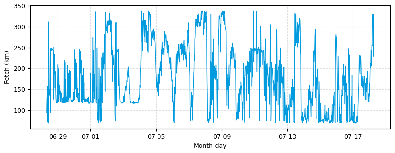
Figure A1 Fetch of the location according to the CenBASE cruise track. It is estimated based on the length to the land and the wind direction.

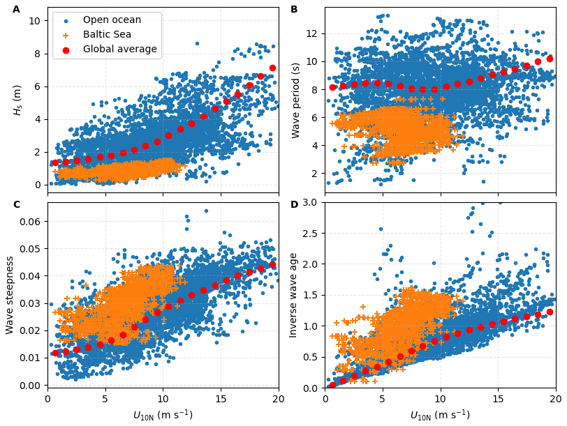
Figure A2 Wave properties versus wind speed. Orange: Waves in the Baltic Sea during CenBASE; Blue: Waves in open ocean cruises with eddy covariance measurements (see Yang et al., 2022); and Red: Waves in the global ocean average. For the global ocean average, we use the year 2024 as an example and take the first day of each month at 00:00 UTC to capture seasonal variability. (A) Significant wave height; (B) Wave period; (C) Wave steepness; (D) Inverse wave age. See Sect. 2.3 of the Method for information on wave data extraction.

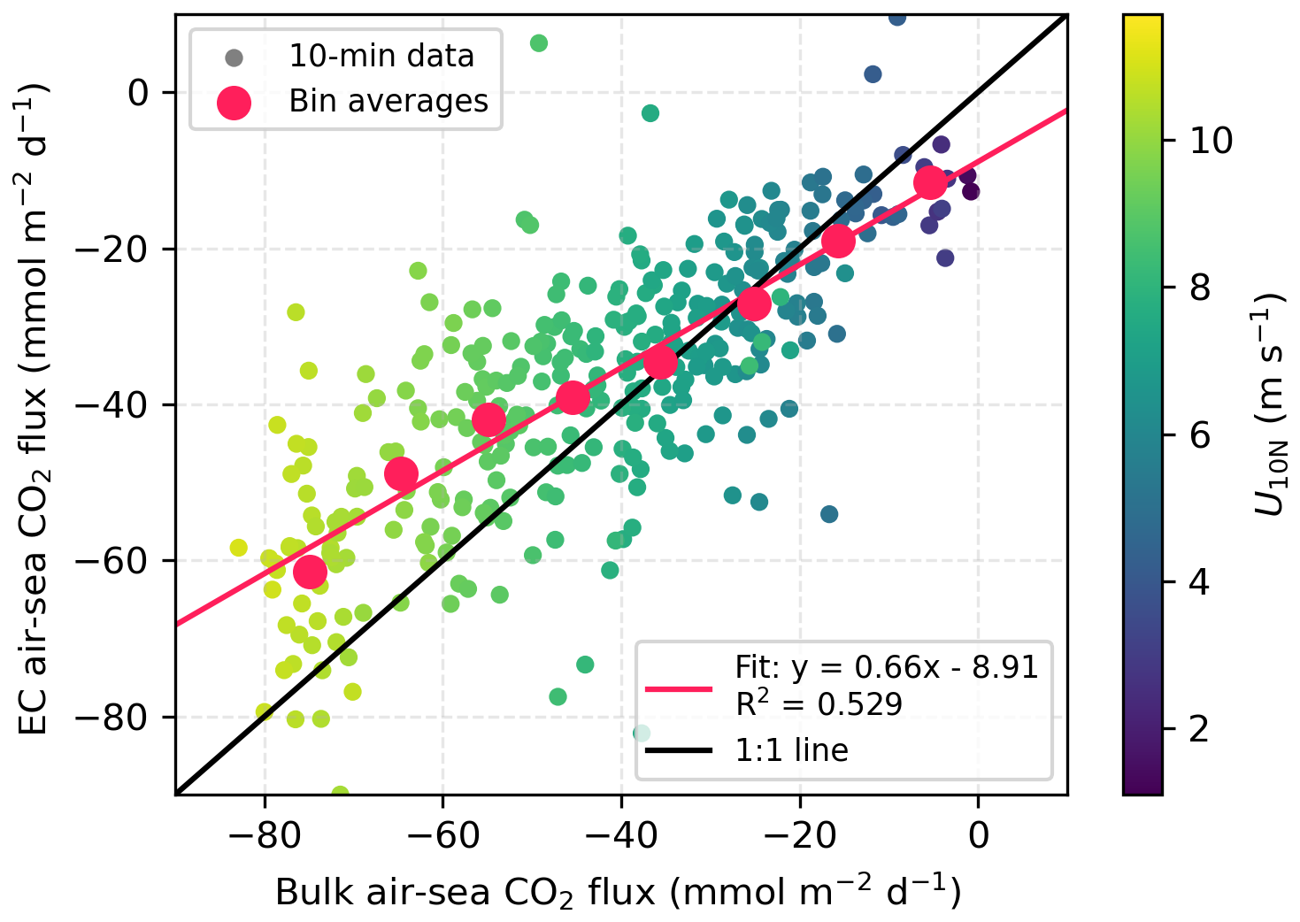
Figure A3 Bulk air–sea CO₂ flux estimates versus EC air–sea CO₂ flux observations. The Ho et al. (2006) parameterisation is used for the bulk flux estimate. The small dots are 10 min flux data, and the large red dots represent the bin averages for every 10 $\mathrm{mmol}{\mathrm{m}}^{-\mathrm{2}}{\mathrm{d}}^{-\mathrm{1}}$ flux interval. The EC flux observations are lower in magnitude than the bulk flux estimates at wind speeds higher than ∼ 7 m s⁻¹.

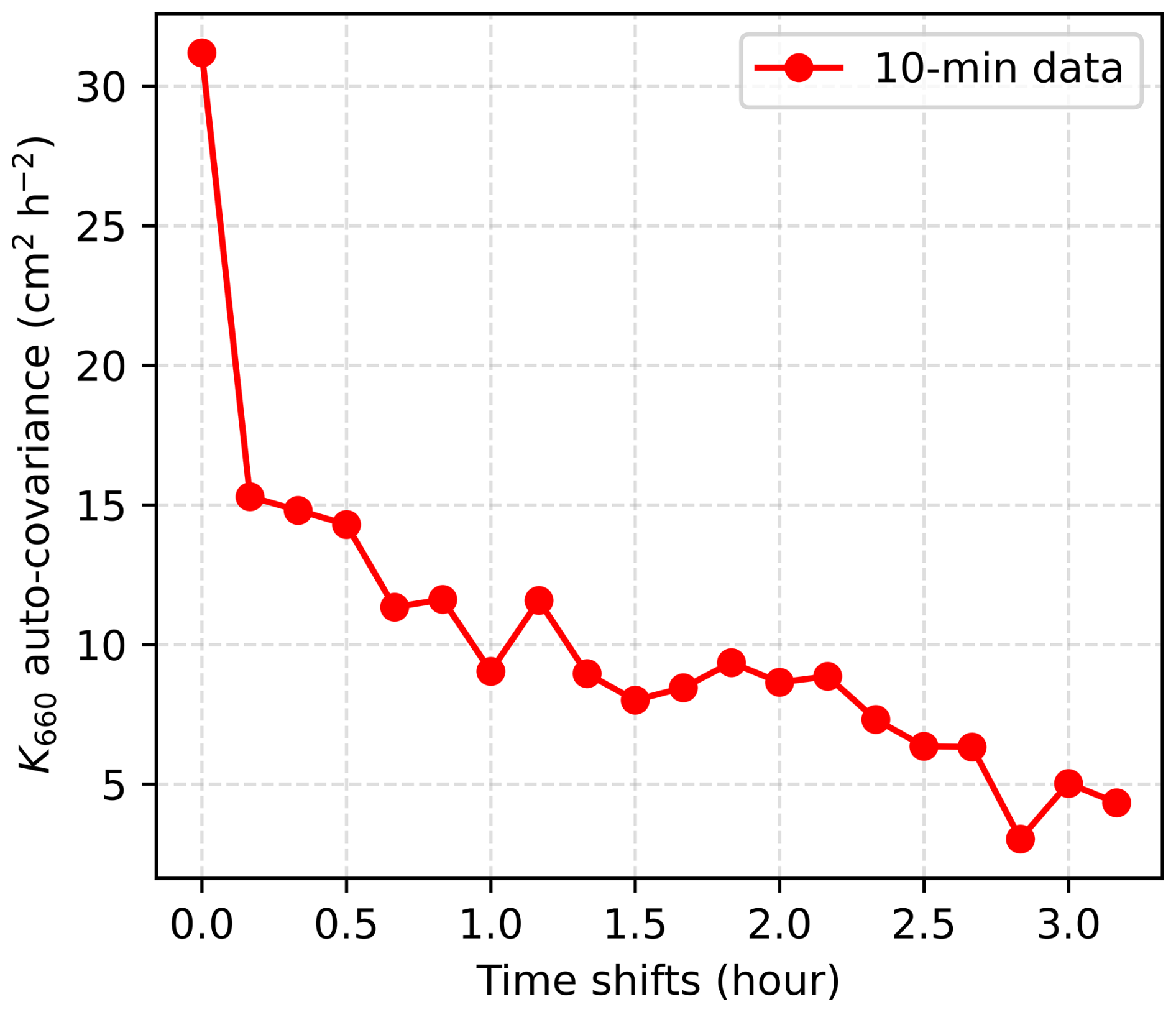
Figure A4 Auto-covariance of EC-derived CO₂ transfer velocities (K₆₆₀). The 10 min K₆₆₀ time series from 4–7 July, selected for its continuity (see Fig. 1F), was used for this analysis. The first point represents the variance of the K₆₆₀ time series, while the second point shows the covariance between the original series and a version shifted by one point (i.e., 10 min). The decrease from the first to the second point indicates the random uncertainty in this K₆₆₀ time series (∼ 50 %). This uncertainty can be further reduced to ∼ 20 % for a 1 h average (i.e., $\mathrm{50}\mathit{\%}/\sqrt{\mathrm{6}}$).

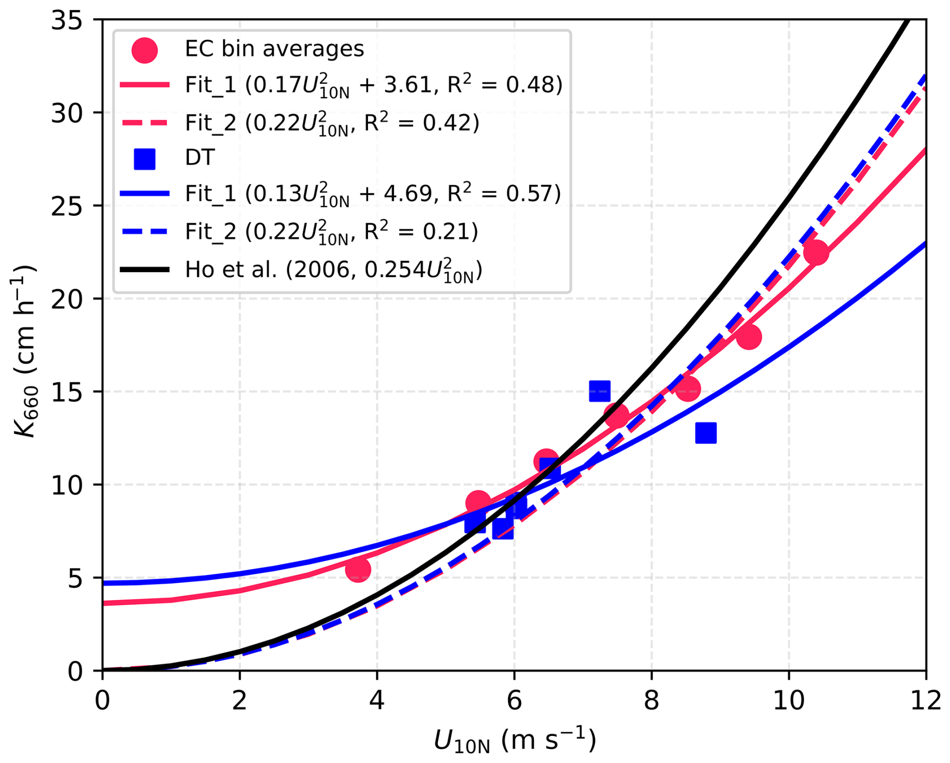
Figure A5 Observed and parameterised gas transfer velocities (K₆₆₀). Red dots show 10 min EC-derived bin averages (for each 1 m s⁻¹ U_10N bin), with red lines representing parameterisations fitted to these data. Blue squares denote DT-derived K₆₆₀ values (timescale ∼ 1 d), with blue lines showing corresponding parameterisations. Solid lines follow the fitting form $K_{\mathrm{660}}=a{U}_{\mathrm{10}\mathrm{N}}^{\mathrm{2}}+b$, while dashed lines follow $K_{\mathrm{660}}=a{U}_{\mathrm{10}\mathrm{N}}^{\mathrm{2}}$.

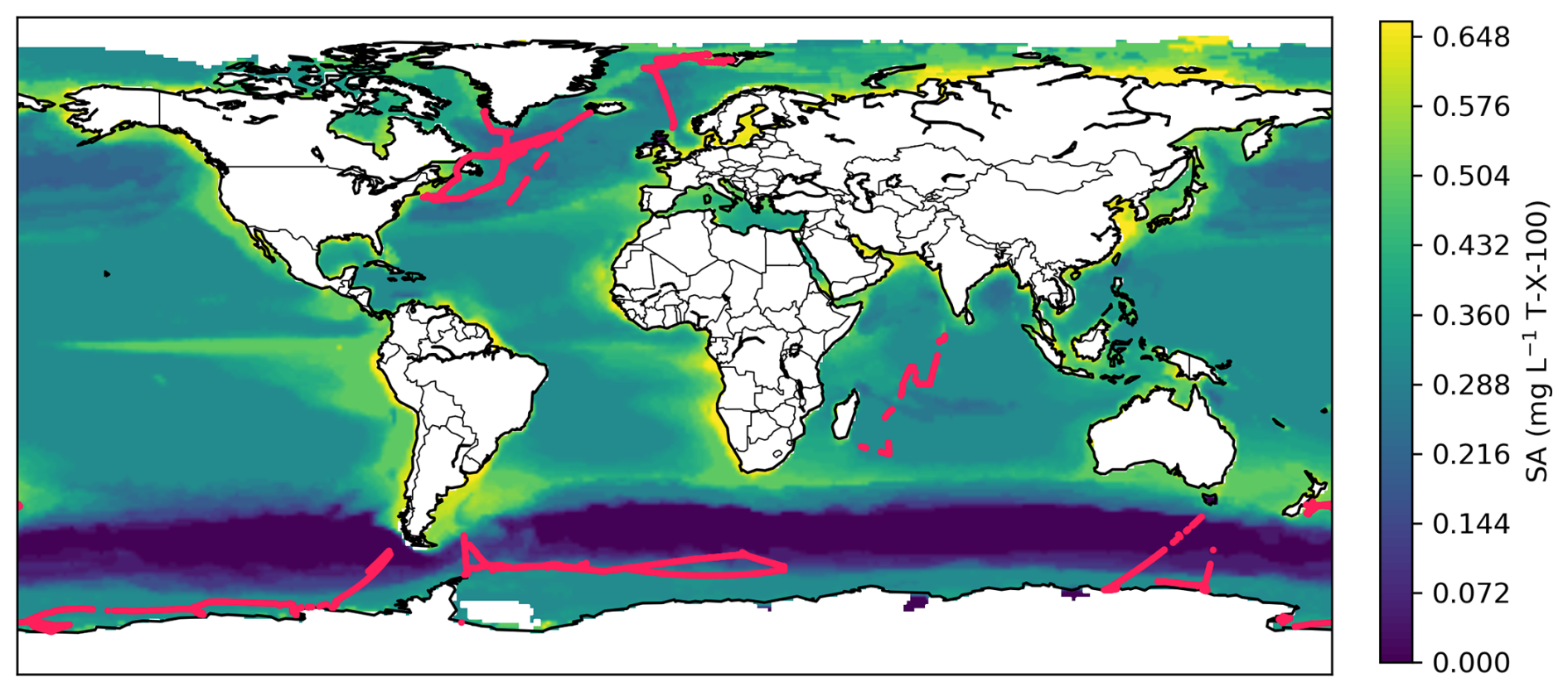
Figure A6 Estimated surfactant distributions in the global ocean and the open ocean EC cruise tracks. The surfactant concentration is estimated following Wurl et al. (2011) shown here as an annual mean. Red lines indicate the EC cruises that were synthesized in Yang et al. (2022).

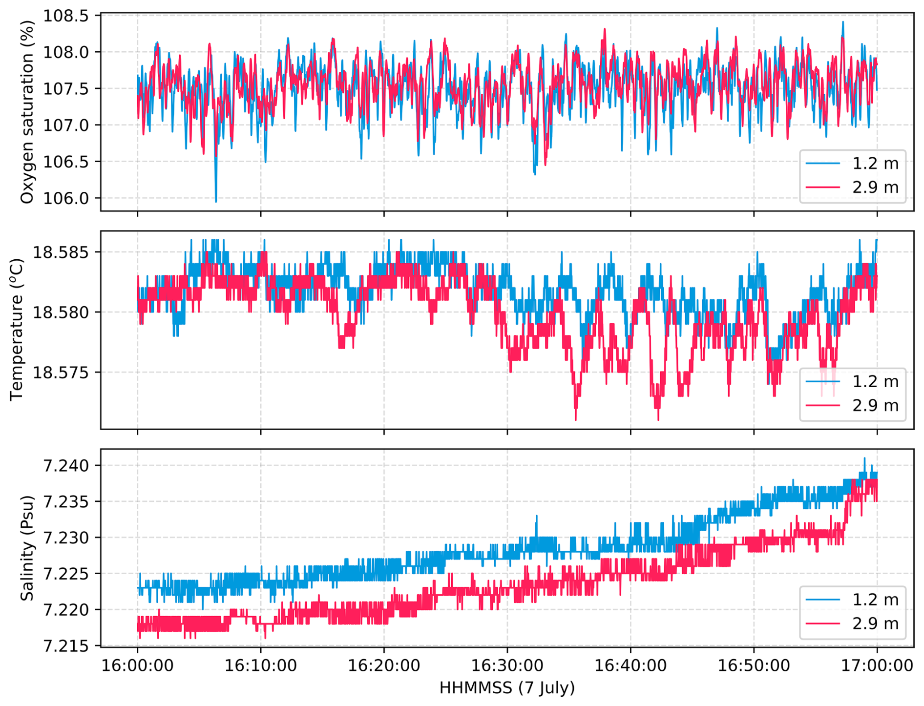
Figure A7 Representative dissolved oxygen, salinity and temperature data from the small spar buoy, showing the differences measured at 1.2 and 2.9 m depth. The patterns shown here are typical of both day and night measurement periods. The time shown here represents the UTC time.

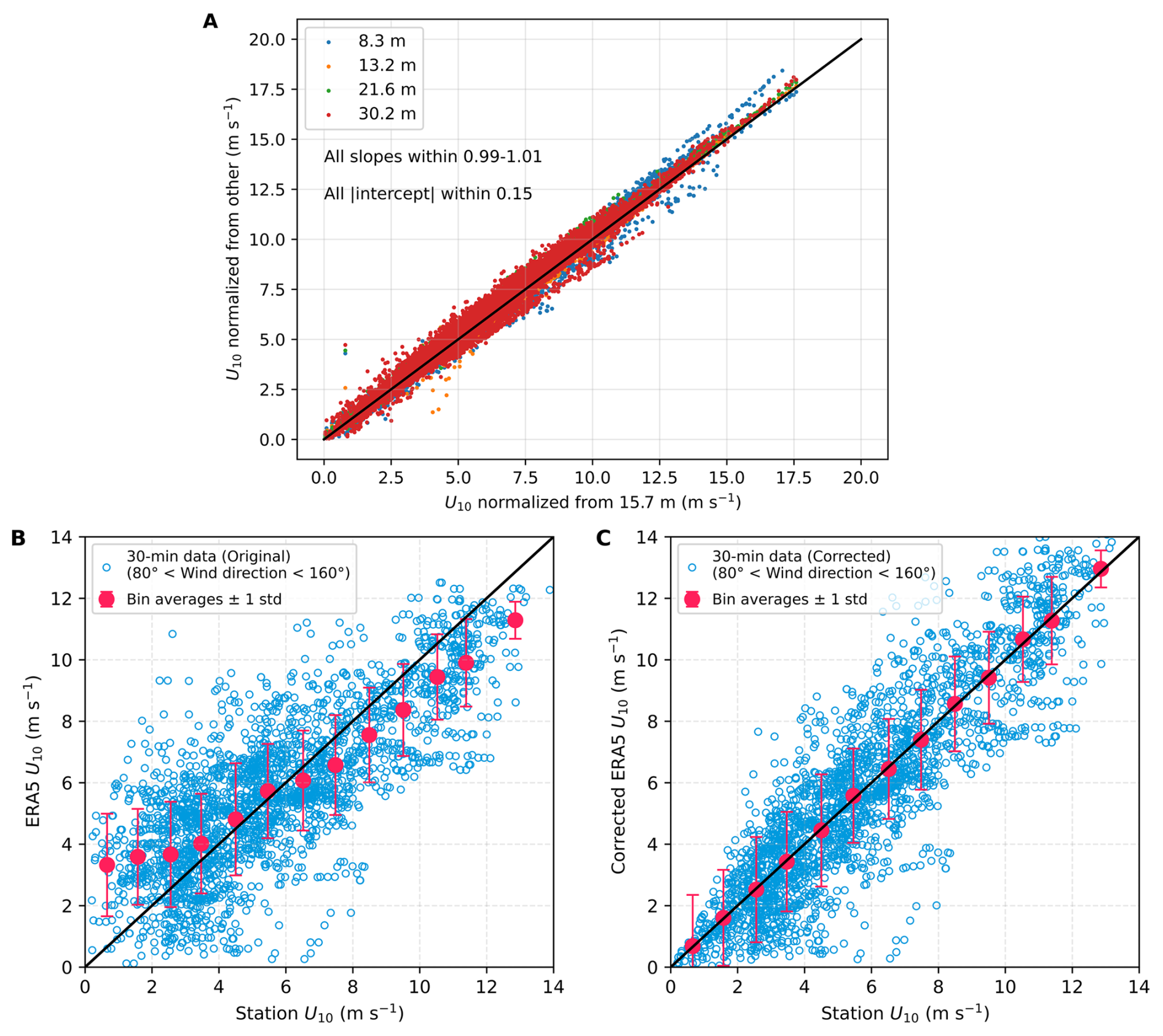
Figure A8 Correction of ERA5 wind speed using reference measurements from the Östergarnsholm station (restricted to the open sector, 80–160°; Rutgersson et al., 2020). (A) Comparison of the wind speed measurements from different heights at the Östergarnsholm station. All wind speeds were normalized to 10 $\mathrm{m}\mathrm{a}.\mathrm{m}.\mathrm{s}.\mathrm{l}.$ (U₁₀). (B) Comparison of the station U₁₀ measurements and the extracted ERA5 U₁₀ at the location of the Östergarnsholm station. The red points are bin averages with error bars representing 1 standard deviation. The red points in panel (B) are fitted with 2 linear relationships: (1) $y=\mathrm{0.64}x+\mathrm{2.05}$ for station U₁₀ < 7.5 m s⁻¹, and (2) $y=\mathrm{0.88}x+\mathrm{0.28}$ for station U₁₀ > 7.5 m s⁻¹ for correction. (C) Comparison of the station and ERA5 U₁₀ after the corrections using the relations in panel (B).

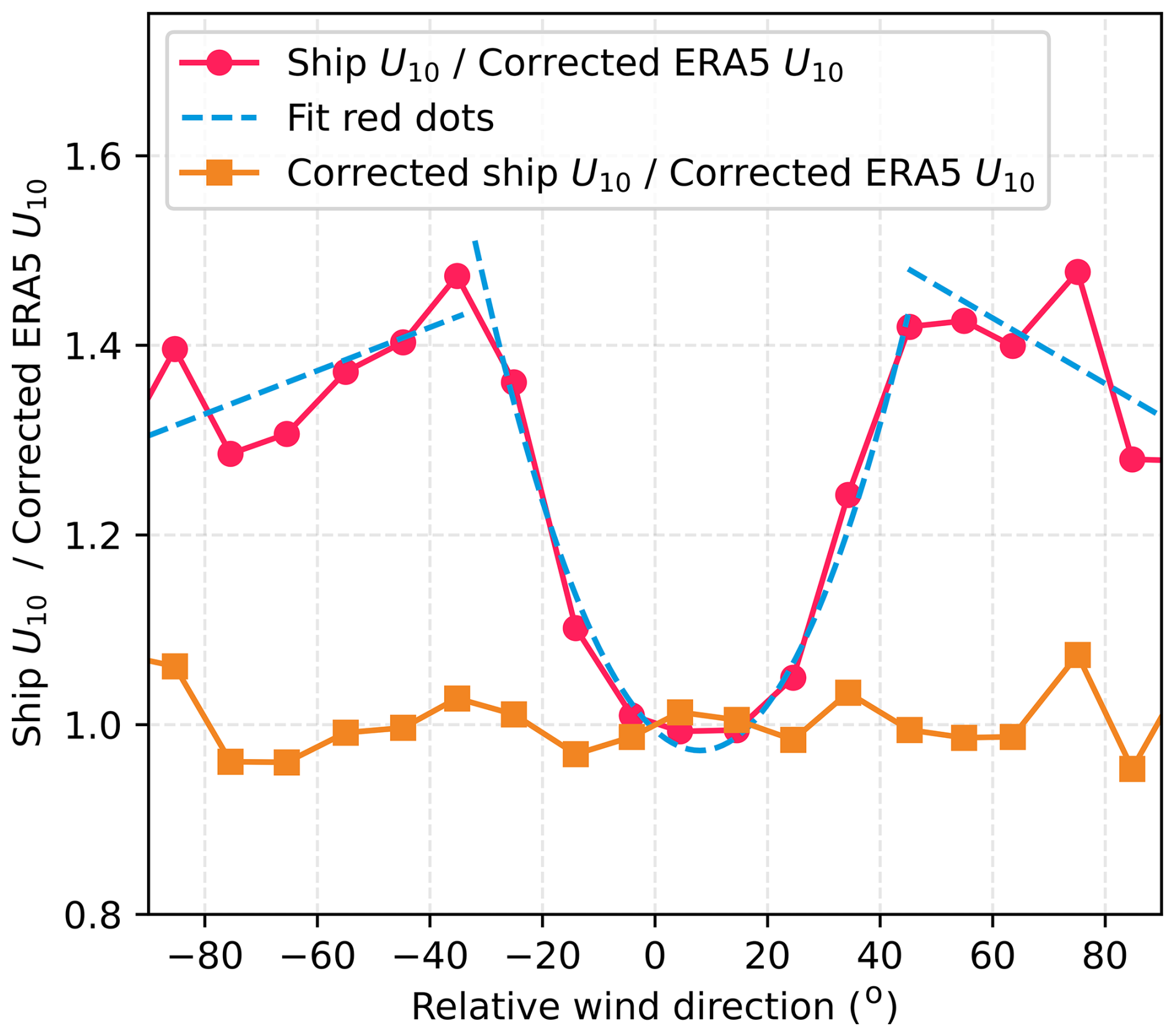
Figure A9 Ratio of ship wind speed to subsampled ERA5 wind speed before (red) and after correction (yellow) as a function of relative wind direction (RWD). ERA5 wind speeds were first calibrated against the Östergarnsholm station record (Fig. A8). The fitted relationships (blue) are: (1) $y=\mathrm{0.00036}(\text{RWD}-\mathrm{8}{)}^{\mathrm{2}}+\mathrm{0.97}$ for −30 to 45°, (2) $y=\mathrm{0.0023}\text{RWD}+\mathrm{1.51}$ for −90 to −30°, and (3) $y=-\mathrm{0.0035}\mathrm{RWD}+\mathrm{1.64}$ for 45 to 90°.