Turbulent atmospheric particle fluxes in the High Arctic: surface type dependence and variability

The Arctic is warming at a significantly faster rate than the global average. This is altering the sources and sinks of aerosols, which influence the regional radiation balance and cloud formation. However, direct observations of turbulent particle fluxes over sea ice are scarce, limiting our understanding of the processes that control the exchange of aerosols between the surface and the atmosphere. During the ARTofMELT campaign in spring 2023, five weeks of continuous eddy covariance measurements of turbulent particle fluxes were conducted in the High Arctic to investigate particle sources and sinks over closed ice, leads, and open water. Overall, net particle deposition dominated, with median deposition fluxes of −0.02 (interquartile range −0.10 to 0.04) × 10⁶ m⁻² s⁻¹ over closed ice. This confirms the role of ice surfaces as a particle sink under low to moderate turbulence. Under strong winds, net particle emission fluxes of up to 0.98×10⁶ m⁻² s⁻¹ (95 % confidence interval excluding zero) were observed over closed ice surfaces, which are likely linked to processes involving blowing snow. A mixture of emission and deposition was observed over leads and open water surfaces. These observations highlight how surface heterogeneity and turbulence intensity can influence particle exchange in the High Arctic. As sea ice retreats and the extent of open water increases, local particle sources are expected to become more relevant to Arctic aerosol budgets and cloud processes. The results provide observational constraints on particle fluxes and may help to reduce related uncertainties in Arctic aerosol and climate model simulations.

1 Introduction

The Arctic is experiencing climate change at a significantly faster rate than the global average (Westergaard-Nielsen et al., 2018; Meredith et al., 2019; You et al., 2021; Rantanen et al., 2022). Since 1979, warming has occurred two to seven times faster than the global rate, with the most pronounced changes in the Eurasian sector, particularly the Barents Sea region (Rantanen et al., 2022). This accelerated warming, also known as Arctic amplification (e.g., Wendisch et al., 2019), is closely linked to feedback mechanisms in the climate system and has an impact on weather systems and climate worldwide (Cohen et al., 2014). Aerosol particles, hereafter referred to as particles, play a central role in the Arctic climate system (Serreze and Barry, 2011; Arctic Monitoring and Assessment Programme, 2021). They influence the energy balance directly by scattering and absorbing solar radiation, and indirectly by acting as cloud condensation nuclei or ice nucleating particles (Twomey, 1977; Albrecht, 1989; Carslaw et al., 2013). As particle concentrations in the Arctic are frequently low, particularly in autumn (Tunved et al., 2013), even small changes can impact cloud formation and radiative processes (Mauritsen et al., 2011; Stevens et al., 2018). Furthermore, recent studies have demonstrated that Aitken mode particles (<70 nm) can act as cloud condensation nuclei under conditions of sufficiently high supersaturation and low accumulation mode particle concentrations (Baccarini et al., 2020; Karlsson et al., 2022). Therefore, understanding the processes controlling particle sources and sinks is essential for improving our knowledge of Arctic aerosol cloud interactions.

The Arctic is strongly influenced by the long-range transport of anthropogenic aerosols, especially in winter and spring. This phenomenon is known as Arctic haze (e.g., Shaw, 1995). During the summer months, large scale atmospheric circulation patterns shift, reducing the influence of long range transport to the High Arctic. At the same time, more frequent precipitation enhances wet scavenging, leading to lower aerosol particle concentrations in the boundary layer. Consequently, local Arctic sources can play a comparatively more important role (e.g., Law and Stohl, 2007; Garrett et al., 2010; Schmale et al., 2022). These local sources include secondary aerosol formation from marine precursor gases (e.g., Heintzenberg et al., 2015), emissions from open leads and associated sea spray production (e.g., Lapere et al., 2023), terrestrial emissions (e.g., Bullard et al., 2016), and biological sources from both sea ice margins and terrestrial environments (e.g., Moschos et al., 2022; Pereira Freitas et al., 2023; Tobo et al., 2024). However, the individual contributions of these sources to total particle number concentration remain unclear. The climatic relevance of different particle types is not necessarily reflected in their number concentration. Newly formed particles may dominate in number, but their impact on aerosol cloud interactions depends on subsequent growth to sizes large enough to activate as cloud condensation nuclei (e.g., Kulmala et al., 2004; Spracklen et al., 2008). Conversely, ice nucleating particles occur at very low concentrations and can nonetheless exert a strong influence on cloud properties (e.g., Kanji et al., 2017; Creamean et al., 2022). The relative contributions of different sources to total aerosol particle number concentration remain uncertain, which leads to uncertainties when quantifying their regional climate impacts (Chylek et al., 2016; Song et al., 2022).

The knowledge of the processes controlling aerosol abundance in the Arctic remains incomplete, particularly with regard to emissions, transport, transformation, and removal (Korhonen et al., 2008; Willis et al., 2018). These gaps hinder the representation of accurate aerosol-climate interactions. While aerosol microphysical properties and processes are important for these simulations, their quantitative contribution to uncertainties in simulated Arctic aerosol concentrations remains poorly constrained (Matsui and Liu, 2022). Incomplete emission inventories also contribute to these uncertainties (Whaley et al., 2022; Koike et al., 2025). Furthermore, dry deposition depends on the physical properties of the particles, meteorological and surface specific factors (Donateo and Contini, 2014; Mohan, 2015; Farmer et al., 2021; Donateo et al., 2023). As Willis et al. (2018) and Schmale et al. (2021) point out, very few measurements of the turbulent flux of particles and aerosol precursor gases have been taken in the Arctic to date. Such measurements are crucial for modeling aerosol formation and emissions. Therefore, accurate quantification of vertical turbulent particle fluxes is required to enhance our understanding of the local particle budget in the High Arctic (Saylor et al., 2019).

Initial evidence of local aerosol sources over open leads was described by Scott and Levin (1972), and the first quantitative particle flux measurements in the High Arctic were provided by Nilsson and Rannik (2001) and Nilsson et al. (2001). Subsequent measurements were conducted by Held et al. (2011a, b), Donateo et al. (2023, 2025), Mathes et al. (2025) and Simon et al. (2025). Comparable measurements also exist from Antarctica (Grönlund et al., 2002; Contini et al., 2010). However, the available measurements are sparse, particularly over sea ice, and additional, more extensive datasets are still required. Furthermore, while many studies focus on particle deposition, comparatively few address both emission and deposition fluxes. Conducting eddy covariance measurements poses considerable challenges. On the one hand, a temporal resolution of about 10 Hz is needed to capture small-scale turbulent fluctuations. On the other hand, low particle concentrations and instrumental limitations make detection difficult (Donateo and Contini, 2014). The gradient method is an alternative to eddy covariance. It is based on flux profile relationships and requires a lower instrumental time response but relies upon the assumptions underlying Monin-Obukhov surface layer similarity being valid (Petelski and Piskozub, 2006; Held et al., 2011b; Foken and Mauder, 2024).

This study examines the surface dependent variability of particle sources and sinks in the Arctic Ocean. It is based on a continuous eddy covariance dataset covering five weeks of turbulent particle flux measurements in the High Arctic. Previous ship based eddy covariance studies in the Arctic have typically covered periods ranging from approximately 5 d (Nilsson et al., 2001) to about two weeks (Held et al., 2011a). Although longer measurements of several months have been reported, these were conducted at fixed land based sites in the polar region rather than over the Arctic Ocean (Grönlund et al., 2002; Donateo et al., 2023, 2025). Direct observations of particle exchange between the surface and the atmosphere are still scarce in the Arctic, and the mechanisms influencing vertical particle exchange are not yet fully understood. Fluxes are classified according to three surface types: open water, leads, and closed ice. This allows us to evaluate the impact of surface conditions on particle exchange and identify the circumstances in which the Arctic Ocean surface acts as a net source or sink of particles. The results provide observational data that may help reduce uncertainties related to particle fluxes in Arctic model simulations.

2 Data and methods

This work is based on data collected during the ARTofMELT (Atmospheric Rivers and the Onset of Arctic Sea Ice Melt) expedition, which took place in the Arctic Ocean in spring 2023 aboard the Swedish icebreaker Oden. The primary objective of the campaign was to improve our understanding of the processes that trigger the onset of sea ice melt and to investigate its connection to atmospheric rivers, which carry warm, moist air poleward in narrow corridors (Swedish Polar Research Secretariat, 2024; Tjernström and Zieger, 2025). The expedition embarked from Svalbard on 8 May 2023 and concluded there on 15 June 2023. After departure from Longyearbyen, Oden headed northwest towards the marginal ice zone and into the pack ice. The expedition then followed the route in Fig. 1, encountering varying surface conditions with sea ice, leads and open water. During two extended ice camps, Oden was moored to an ice floe and drifted with the ice. The first ice camp took place from 16 to 21 May 2023 at 79.6° N, 1.3° W, and the second from 29 May to 11 June 2023 at 79.8° N, 2.8° E. After the second ice camp, Oden returned through the marginal ice zone before heading back to Svalbard.

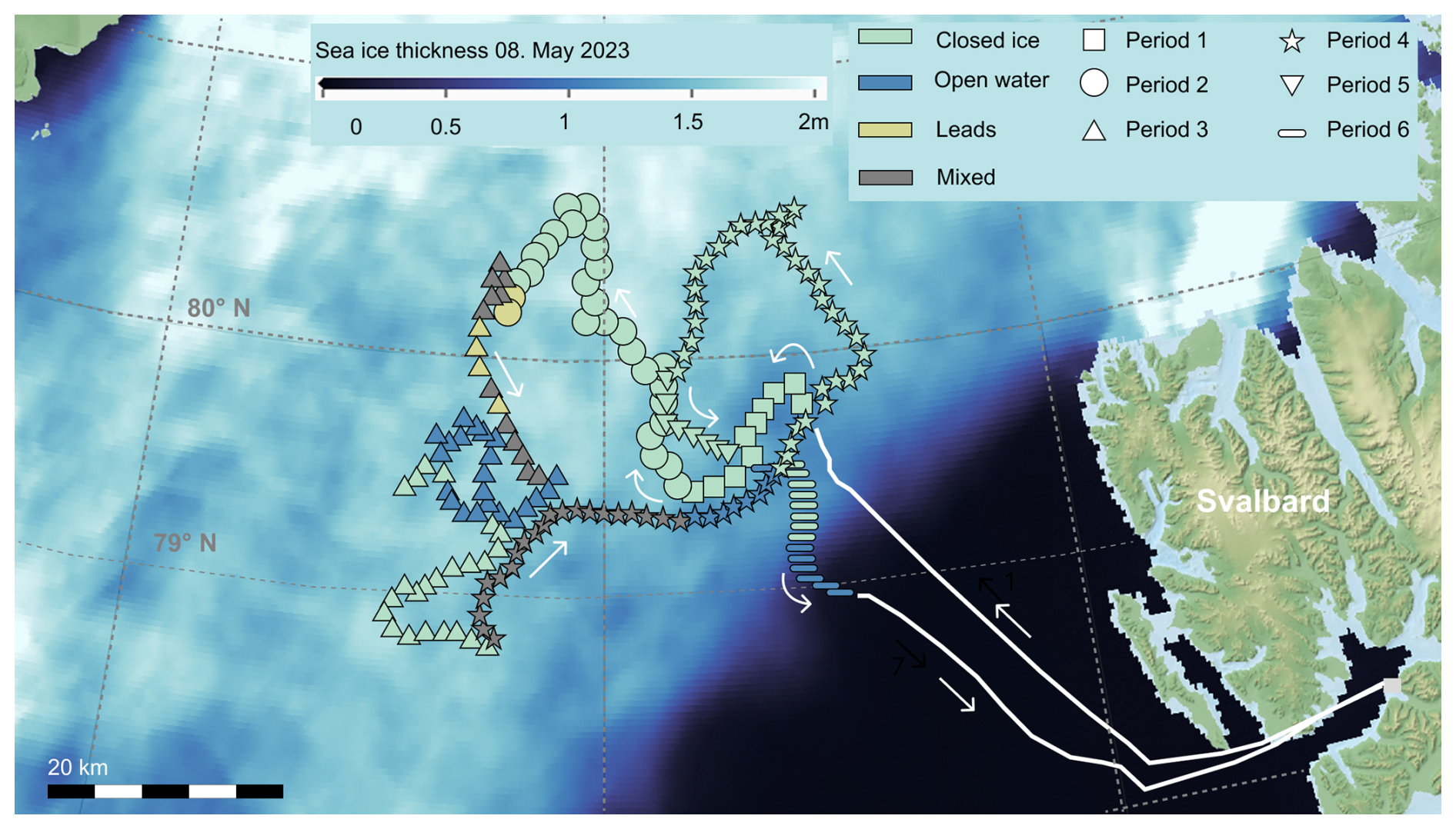
Figure 1 Expedition track of the ARTofMELT campaign overlaid on sea ice thickness on 8 May 2023. The different symbols indicate the meteorological periods. Colors show the dominant surface type. The white sections of the track indicate periods for which no surface type information was available, corresponding to the transit into and out of the sea ice. The arrows indicate the direction of travel along the expedition track. Sea ice thickness data © Copernicus Marine Service (CMEMS), 2023.

This manuscript presents eddy covariance particle fluxes, which were continuously measured on Oden's foremast between 10 May and 12 June 2023. Additional measurements of particle number concentrations and meteorological parameters were used for data interpretation. Profiles of temperature, humidity, and wind speed were obtained from radiosonde weather balloons, launched every 6 h (Murto et al., 2024b). Near-surface meteorological conditions were obtained from a weather station deployed on the 7th top deck (Murto et al., 2024a). The analysis focuses on the potential dependence of turbulent particle fluxes on the surface type. Based on hourly images taken on the seventh deck, the surface was divided into three categories:

1. closed ice: smooth snow-covered ice surfaces without ridges or melt ponds (e.g., Fig. 2a);

2. open water: extensive open water and wide lead surfaces (e.g., Fig. 2b);

3. lead: open water within leads or thin ice within pack ice (e.g., Fig. 2c).

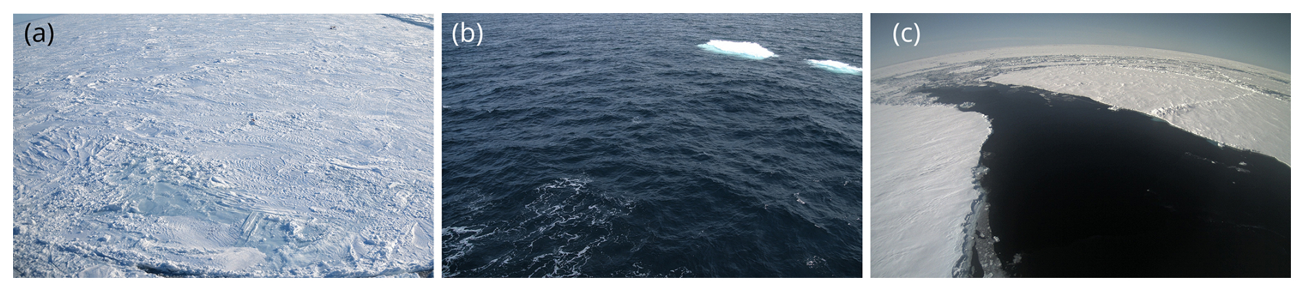
Figure 2 Example pictures from the automatic camera showing different dominating surface types: (a) closed ice; (b) open water; (c) leads.

Since Oden was typically aligned with the main wind direction for atmospheric measurements, the relative wind direction was most frequently onto the bow (53 % of the measurement campaign, 315 to 45°). The relative wind direction was towards the port side in 19 % of the cases (215 to 314°), and towards the starboard side in 21 % of the cases (46 to 145°) (Murto et al., 2024a). The remaining percentage represents wind onto the aft deck, but these periods are typically affected by ship exhaust and are therefore discarded from further analysis.

2.1 Sampling methodology

Turbulent particle fluxes were measured by eddy covariance using a sonic anemometer (uSonic-3, Metek, Elmshorn, Germany) and a mixing-type condensation particle counter (MCPC 1720, Brechtel, Hayward, CA, USA). The sonic anemometer measured three-dimensional wind components and sonic temperature at an acquisition rate of 40 Hz. It was installed on the foremast, 20.3 m above the water or ice surface, over the Oden's bow (Fig. A1). For particle measurements, an aluminium box housing the MCPC was installed at the bottom of the foremast (Fig. A1c and d). The box was heated to 15 °C to ensure stable instrument operation, while the sampling lines inside the box were kept as short as possible to reduce residence time and thereby minimize potential evaporation. The inlet of the MCPC sampling line was positioned directly next to the sonic anemometer (Fig. A1e).

At the top of the foremast, the sampling line started with 10 cm of conductive tubing with an inner diameter of 6.2 mm, oriented downward to protect the sampling line from precipitation. From there, 11.2 m of stainless steel tubing with an inner diameter of 4.5 mm ran downward along the foremast to the mast base. The final section consisted of 2.8 m of conductive tubing with an inner diameter of 4.2 mm, connecting the mast base to the MCPC box located at the bottom of the foremast. A bypass system was used due to the long sampling line to obtain a total flow rate of approximately 5.5 L min⁻¹ in the sampling line. Part of the flow was diverted around the MCPC via an auxiliary flow path driven by a second vacuum pump, and then recombined downstream (Philipp Oehlke, personal communication, 2026). This increased the inlet flow velocity and reduced residence time. Butanol was used as the working fluid in the MCPC, and was then removed from the exhaust gas using activated charcoal. The MCPC measured particle number concentrations with a lower cutoff diameter of 7 nm. According to the manufacturer, the nominal response time of the MCPC is 180 ms, corresponding to a high frequency sampling cut off at 5.6 Hz. Particle counts were recorded at 20 Hz. The particle number concentration was calculated and corrected using the simultaneously logged 1 Hz particle counts and flow data. The sensible heat flux was calculated from the sonic anemometer measurements of vertical wind velocity and sonic temperature. Absolute air temperature and relative humidity were measured with an aspirated sensor at the top of the foremast (MP101, Rotronic, Hauppauge, NY, USA). Together with height-adjusted air pressure measurements from the seventh deck weather station, these data were used to calculate air density. The raw heat flux was corrected for the contribution from the latent heat flux, which was estimated using water vapor measurements from an open-path LI-7500 gas analyzer (LI-COR Biosciences, Lincoln, NE, USA).

Hourly images of the ship's surroundings, which were used to classify the surface types, were captured using three Mobotix M24 IP cameras (Mobotix M24 IP, Langmeil, Germany). These were installed on the seventh deck of the Oden, facing the port side, starboard side, and bow. For each surface classification, an image was selected from the camera facing the upwind fetch according to the relative wind direction averaged over 1 h.

2.2 Data analysis

2.2.1 Particle concentration data

The measured particle number concentrations were corrected for particle loss occurring in the sampling inlet. In particular, small particles are lost through diffusion to the tubing and inlet walls (Kulkarni et al., 2011). Diffusional losses in a flow through a circular tube with a uniform inlet were calculated for various particle diameters according to Gormley and Kennedy (1949). To determine the penetration fraction of the ambient particle population, the number size distribution of particles between 15 and 792 nm was taken into account. This was measured with a temporal resolution of 12 min using a differential mobility particle sizer (DMPS) on the fourth deck of Oden, with an inlet at roughly the same height as the mast. Periods influenced by pollution from the ship's exhaust were excluded based on the derivative of the total particle number, following a similar principle as described by Beck et al. (2022). The calculated penetration efficiency was between 25 % for 15 nm particles and 100 % for particles from 240 to 792 nm. The mean penetration efficiency for the total particle population was 95 %.

As the particle fluxes were measured using a closed-path instrument, it was necessary to determine the time lag between fluctuations in the vertical wind component and particle concentration. Based on the pipe length and inner diameter of the inlet tubing, the total inlet tubing volume was estimated to be 0.22 L. With a volume flow rate of 5.5 L min⁻¹, the resulting theoretical travel time is approximately 2.4 s. An additional residence time of approximately 0.6 s within the MCPC was included. This results in an estimated total time lag of 3 s, which was confirmed by covariance maximization.

Data contaminated by ship exhaust were removed. To this end, the relative wind direction with respect to the ship's bow, the particle concentration measured at the foremast using an MCPC, and the particle concentration measured using a CPC in the aerosol container on the fourth deck were evaluated. First, the MCPC and CPC concentrations were averaged to a time resolution of 1 min. A “wind alarm” was triggered when the relative wind direction onto the bow was outside the clean sector of 270 to 90°. A “concentration alarm” was triggered when the CPC in the aerosol container exceeded a threshold concentration. This threshold varied throughout the expedition depending on the ambient background concentration. The following pollution cases were thus defined:

Case A:

At least one alarm was active. The particle concentration of the MCPC exceeded 200 cm⁻³ and was at least 10 % higher than the 20 min mean concentration of the MCPC.

Case B:

At least one alarm was active, and the absolute difference between the particle concentration of the MCPC and the CPC in the aerosol container was less than 200 cm⁻³; the MCPC was more than 20 % above the 20 min mean concentration.

Case C:

At least one alarm was active, and the particle concentration of the MCPC exceeded 800 cm⁻³.

Case D:

The MCPC concentration exceeded 2000 cm⁻³, regardless of any alarm status.

An additional 10 s interval was removed before and after each pollution case to ensure that the polluted air parcel was not included in the analysis. 20 min averaging intervals containing more than 10 % missing data were discarded. Data gaps were not replaced or interpolated. In total, 17 % of the entire measurement data were affected by pollution (including the 10 s buffer) and were removed. Within the fraction of the measurement data affected by pollution, Cases A and C occurred most frequently, at 32 % and 58 %, respectively.

2.2.2 Turbulence data

Turbulent wind measurements made from a moving platform like the foremast of a ship require correction for both their changing orientation and the motion of the platform. 3-axis accelerations and rotation rates were measured at 40 Hz at the base of the sonic anemometer on the foremast (MTi-G-700, XSens, Enschede, NL) and averaged to 20 Hz. These measurements were then combined with lower frequency ship navigation data to calculate corrections for the orientation and motion of the anemometer (Edson et al., 1998; Prytherch et al., 2015). Distortion of the mean flow over the ship's superstructure is corrected using the results of a CFD modeling study of Oden (Moat et al., 2015; Prytherch et al., 2017). After motion correction, double rotation was applied to align the coordinate system with the mean flow streamlines and to ensure a zero mean vertical wind velocity (Wilczak et al., 2001). Wind components were linearly detrended (Moncrieff et al., 2006). In addition, spike count and removal procedures following Mauder et al. (2013) were used. A tolerance level of 1 % was set for accepted spikes and dropouts. The processed wind measurements were averaged to 10 Hz for the turbulence and flux calculations in this study.

Friction velocity (u_*, in m s⁻¹) was calculated as a measure of near-surface turbulence:

$$\begin{array}{}\text{(1)}& {\displaystyle }{u}_{*}={\left[(\stackrel{\mathrm{‾}}{u^{\prime }{w}^{\prime }}{)}^{\mathrm{2}}+(\stackrel{\mathrm{‾}}{v^{\prime }{w}^{\prime }}{)}^{\mathrm{2}}\right]}^{\frac{\mathrm{1}}{\mathrm{4}}}\left[\mathrm{m}{\mathrm{s}}^{-\mathrm{1}}\right].\end{array}$$

u and v (in m s⁻¹) are the horizontal wind components, w (in m s⁻¹) is the vertical wind component. The prime denotes the fluctuation about the mean value, and the overbar denotes the average. The dimensionless parameter $\mathit{\zeta }=z/L$ was used to characterize atmospheric stability, where z is the height and L is the Obukhov length (both in m):

$$\begin{array}{}\text{(2)}& {\displaystyle }L=-{\displaystyle \frac{u_{*}{}^{\mathrm{3}}}{\mathit{\kappa }\frac{g}{T}\stackrel{\mathrm{‾}}{w^{\prime }{T}^{\prime }}}}\left[\mathrm{m}\right]\end{array}$$

where κ=0.4 is the dimensionless von Kármán constant, g=9.81 m s⁻² is the gravitational acceleration, $\stackrel{\mathrm{‾}}{w^{\prime }{T}^{\prime }}$ (in K m s⁻¹) is the covariance of the turbulent fluctuations of vertical wind speed w and sonic temperature T (in K). Near zero values for the dimensionless stability parameter $z/L$ indicate neutral conditions, while positive and negative values indicate stable and unstable stratification, respectively (Sorbjan and Grachev, 2010).

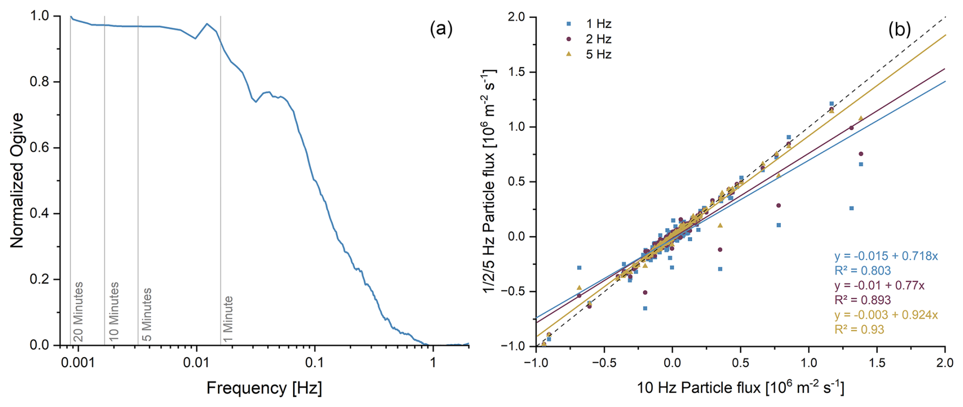
Figure 3 Normalized mean ogive for the particle flux (a), calculated from 10 Hz eddy covariance data. The vertical lines show the frequencies corresponding to 20, 10, 5, and 1 min intervals. Scatter plot (b) of particle number fluxes calculated using 10 Hz data (on x axis) and 1, 2, 5 Hz (on y axis), and linear regressions. The dashed line indicates the 1:1 slope.

2.2.3 Particle flux calculation

Eddy covariance calculations of the particle fluxes were performed using Eddy Pro software (LI-COR, Inc., 2021), employing measured particle concentrations (see Sect. 2.2.1) and the corrected 10 Hz vertical velocities from the foremast turbulence instruments (see Sect. 2.2.2). The direction of the turbulent particle fluxes is defined such that an upward flux is positive and a downward flux is negative. To determine a suitable averaging period for eddy covariance calculations, ogives (i.e., cumulative cospectra representing the contribution of different frequencies to the total flux) were calculated following linear detrending and double rotation of the wind components. To this end, preliminary particle flux calculations and spectral analyses were performed. The mean ogives, averaged over multiple time periods, were normalized to the total particle flux covariance so that they converge to 1 at low frequencies. The choice of an averaging interval was guided by the interpretation of ogive plots, as suggested by Moncrieff et al. (2006). As shown in Fig. 3a, most of the turbulent contributions to the flux are captured within 5 min periods. An averaging interval of 20 min was selected. This allows slightly larger turbulent eddies to be included and averaging over multiple eddies at dominant flux-carrying scales, giving better statistical stability to the flux estimate. At the same time, slower variations that are not related to local turbulent exchange are not considered.

Figure 3b shows results of using different lower sampling frequencies (1, 2, and 5 Hz) compared to 10 Hz, given the effective sampling rate of the MCPC assumed to be 5.6 Hz. The results, indicated by the slopes of the regression lines, show a systematic reduction in turbulent particle fluxes using the lower time resolution. The 5 Hz results are the closest to the 1:1 curve, with a slope of 0.92, indicating a systematic reduction of 8 %. This suggests that the MCPC can measure small-scale turbulent fluctuations of at least 5–10 Hz and that its time response is likely to be within this range. A comparison of the theoretical flux reduction (18 % at 1 Hz, 8 % at 2 Hz, and 2 % at 5 Hz) according to Horst (1997) shows qualitative agreement with the experimental reductions of 29 %, 23 %, and 8 % indicated by the slopes of the linear regressions. High-frequency losses were corrected after Horst (1997), using transfer functions of the eddy covariance system to estimate flux losses analytically, taking into account the measurement height, mean wind speed, system time constant, and stability dependent cospectral parameters. Hence, the covariance fluxes were calculated from vertical winds and aerosol concentration averaged to a frequency of 10 Hz. This captures small-scale turbulent fluctuations in the 5–10 Hz frequency range, while remaining consistent with the effective time response of the MCPC.

The sampling error of the particle fluxes was estimated following Finkelstein and Sims (2001). This approach considers the temporal autocorrelation of turbulence and estimates the number of statistically independent turbulent eddies contributing to each 20 min flux measurement. Consequently, the sampling error after Finkelstein and Sims (2001) reflects the expected variability in the flux estimate resulting from the finite sampling period and the number of independent turbulent events. The median sampling error of the measured particle fluxes following Finkelstein and Sims (2001) was 0.07×10⁶ m⁻² s⁻¹. In extreme cases, this sampling error may be 0.26×10⁶ m⁻² s⁻¹ (95th percentile). The random uncertainty due to limited counting statistics was estimated from the mean particle concentration, the particle sample flow rate, the standard deviation of vertical wind velocity, and the 20 min averaging time following Buzorius et al. (2003). To combine these two error contributions, the sampling error following Finkelstein and Sims (2001) and the random uncertainty due to limited counting statistics following Buzorius et al. (2003) were propagated using the root sum of squares method.

2.2.4 Dry deposition modeling and emission flux calculation

The measured particle fluxes represent a combination of emission and deposition of particles, with positive net fluxes dominated by emission and negative net fluxes by deposition. To separate deposition from potential emission contributions to the measured net particle fluxes, the dry deposition velocity of aerosol particles was calculated using a size resolved resistance model following Zhang et al. (2001) and Emerson et al. (2020). The approach combines gravitational settling with turbulent transfer through the atmospheric surface layer and surface uptake processes. Contrary to the original formulation by Zhang et al. (2001), Brownian diffusion efficiency was parameterized according to the method of Emerson et al. (2020). Previously, this parameterization showed better agreement with observations. Recent developments in dry deposition models have mainly focused on improving deposition over vegetated surfaces by refining impaction and canopy processes (Saylor et al., 2019; Farmer et al., 2021; Pleim et al., 2022). However, observational constraints for smooth ice and open water surfaces remain limited. The median difference between deposition fluxes calculated using the Emerson and Zhang parameterizations was large, with a median value of the absolute differences of 0.62×10⁶ m⁻² s⁻¹.

The modeled deposition velocity V_D(D_p) (in m s⁻¹) for particles of diameter D_p (in nm) is given by:

$$\begin{array}{}\text{(3)}& V_{\mathrm{D}}\left(D_{\mathrm{p}}\right)=v_{\mathrm{g}}\left(D_{\mathrm{p}}\right)+{\displaystyle \frac{\mathrm{1}}{R_{\mathrm{a}}+R_{\mathrm{s}}}}\left[\mathrm{m}{\mathrm{s}}^{-\mathrm{1}}\right]\end{array}$$

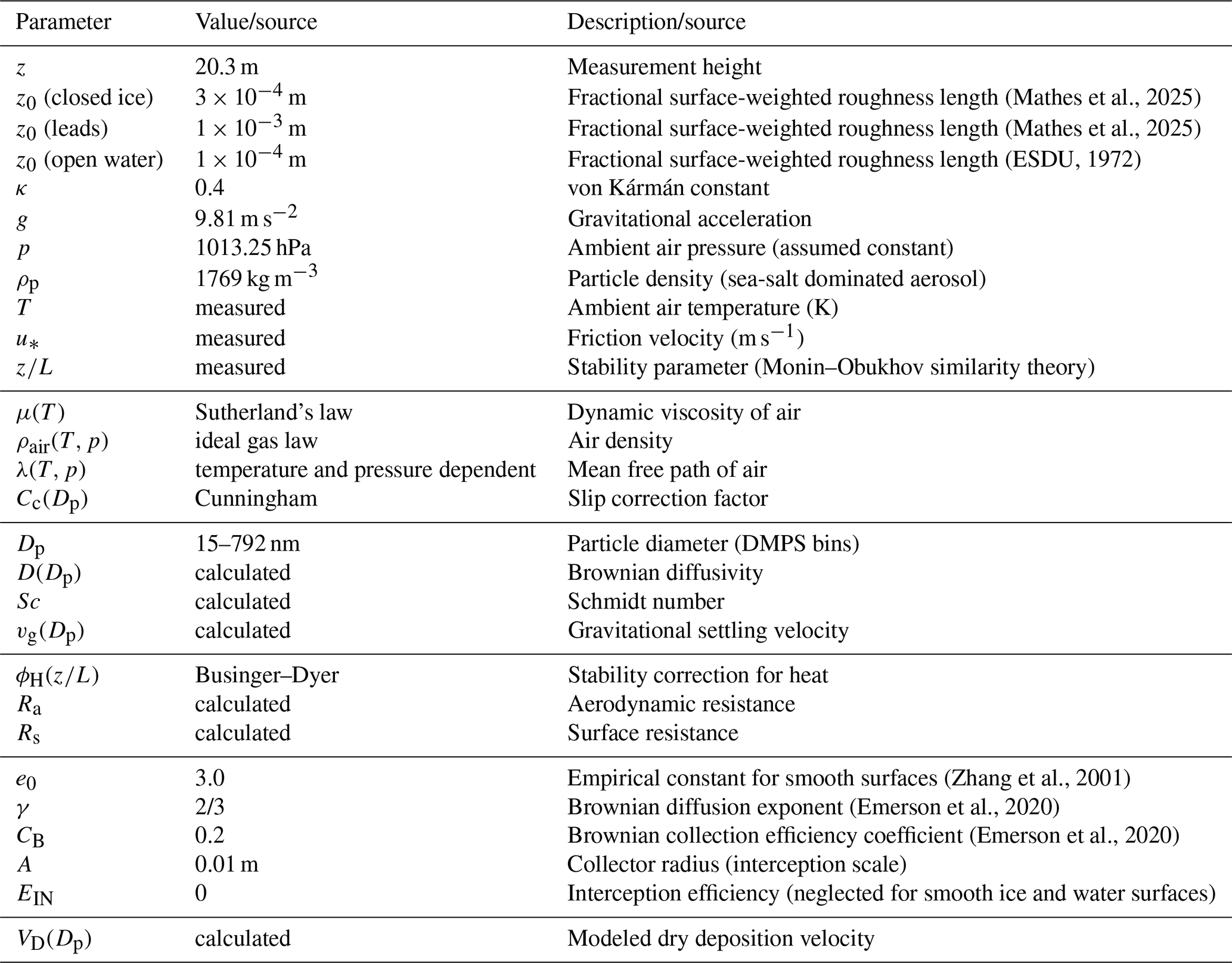
where v_g (in  m s⁻¹) is the gravitational settling velocity, R_a (in s m⁻¹) is the aerodynamic resistance, and R_s (in s m⁻¹) is the surface resistance. Model parameters are summarized in Table A1. The aerodynamic resistance was calculated as:

$$\begin{array}{}\text{(4)}& R_{\mathrm{a}}={\displaystyle \frac{\ln \left(z/z_{\mathrm{0}}\right)}{\mathit{\kappa }{u}_{*}}}{\mathit{\varphi }}_{\mathrm{H}}(z/L)\left[\mathrm{s}{\mathrm{m}}^{-\mathrm{1}}\right]\end{array}$$

where z₀ (in m) is the surface roughness length. z₀ was assigned according to the observed surface types. The effective roughness length (Table A1) was calculated as the fractional area-weighted mean of the individual surface types. A comparison with calculations using a constant z₀ value of 0.009 m showed a median difference in the modeled deposition flux of 0.0016×10⁶ m⁻² s⁻¹, indicating that the results are almost insensitive to z₀.

ϕ_H is a dimensionless stability correction function depending on the stability parameter $z/L$. Stability corrections follow standard Businger–Dyer formulations, and extreme values of $z/L$ were limited to the range [−5, 5] for numerical stability. The surface resistance was calculated as:

$$\begin{array}{}\text{(5)}& R_{\mathrm{s}}={\displaystyle \frac{\mathrm{1}}{e_{\mathrm{0}}{u}_{*}\left(E_{\mathrm{B}}+E_{\mathrm{IM}}+E_{\mathrm{IN}}\right)R_{\mathrm{1}}}}\left[\mathrm{s}{\mathrm{m}}^{-\mathrm{1}}\right]\end{array}$$

where e₀ is an empirical, dimensionless collection efficiency constant for smooth surfaces after Zhang et al. (2001), and E_B, E_IM, and E_IN (dimensionless) represent collection efficiencies due to Brownian diffusion, inertial impaction, and interception, respectively. The dimensionless term $R_{\mathrm{1}}=\exp (-\sqrt{St})$ accounts for reduced collection efficiency at low Stokes numbers, with the Stokes number defined as:

$$\begin{array}{}\text{(6)}& St={\displaystyle \frac{v_{\mathrm{g}}{u}_{*}^{\mathrm{2}}}{g\mathit{\nu }}}\left[\mathrm{dimensionless}\right]\end{array}$$

where ν (in m² s⁻¹) is the kinematic viscosity of air. In contrast to the original formulation by Zhang et al. (2001), the Brownian diffusion efficiency was parameterized following Emerson et al. (2020), using:

$$\begin{array}{}\text{(7)}& E_{\mathrm{B}}=C_{\mathrm{B}}S{c}^{-\mathit{\gamma }}\left[\mathrm{dimensionless}\right]\end{array}$$

where Sc is the dimensionless Schmidt number and C_B and γ are constants, adopted to better represent particle transfer over smooth ice and water surfaces (Table A1). The Schmidt number was calculated as:

$$\begin{array}{}\text{(8)}& Sc={\displaystyle \frac{\mathit{\nu }}{D}}\left[\mathrm{dimensionless}\right]\end{array}$$

where ν is the kinematic viscosity of air (m² s⁻¹) and D is the particle Brownian diffusivity (m² s⁻¹). The inertial impaction efficiency was calculated as:

$$\begin{array}{}\text{(9)}& E_{\mathrm{IM}}={\displaystyle \frac{S{t}^{\mathrm{2}}}{\mathrm{400}+S{t}^{\mathrm{2}}}}\left[\mathrm{dimensionless}\right].\end{array}$$

Particle loss due to interception (E_IN) is not taken into account in the applied model, because interception is only parameterized for surfaces with collectors, which is not applicable for ice and water surfaces (Zhang et al., 2001; Emerson et al., 2020). The gravitational settling velocity was calculated assuming Stokes flow with Cunningham slip correction. Air viscosity, density, and mean free path were computed as functions of temperature and pressure. The size-resolved deposition flux for each diameter bin was calculated as:

$$\begin{array}{}\text{(10)}& F_{\mathrm{dep},i}=-V_{\mathrm{D}}\left(D_{\mathrm{p},i}\right)C_i\left[{\mathrm{m}}^{-\mathrm{2}}{\mathrm{s}}^{-\mathrm{1}}\right]\end{array}$$

where C is the particle number concentration (in m⁻³) in size bin i, taken from the DMPS measurements on the fourth deck. The total modeled deposition flux was obtained by summing over all size bins from 15 to 792 nm. The inferred emission strength was defined as the difference between the measured net particle flux and the modeled deposition flux. Positive values indicate periods during which particle emission at the surface is inferred. Negative values indicate periods during which the measured net particle flux is smaller than the modeled dry deposition. Uncertainties of both the measured net particle flux and the modeled deposition flux can lead to negative inferred emission fluxes, which indicate periods without particle emission or very low particle emission, typically within the estimated flux uncertainty.

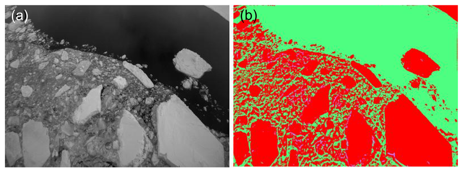
Figure 4 Example of surface type characterization, showing the (a) cropped camera image and the (b) analyzed surface types. Thick ice is displayed in red, open water in green, and thin ice in purple.

2.2.5 Surface characterization

The surrounding surface types were automatically evaluated using a random forest algorithm implemented in the Trainable WEKA Segmentation plugin (Waikato Environment for Knowledge Analysis) within the Fiji distribution of ImageJ (Schneider et al., 2012; Schindelin et al., 2012; Arganda-Carreras et al., 2017) and applied to an image of the surface taken every hour. Depending on the direction of the wind in relation to the ship's position, one of three image orientations was selected to define the surface type located upstream. For each hourly surface classification, a single image from the camera facing the upstream fetch was analyzed. The data on the relative wind direction was also averaged over a period of 1 h. Image processing macros within Fiji were used for the surface type analysis and to tilt, crop, and resize the images. The Trainable WEKA Segmentation plugin was chosen because it performs supervised, pixel based image classification. It uses manually labeled training data to train a classifier that can then be used to automatically classify the remaining images. Several commonly used image segmentation approaches (Minaee et al., 2022) were evaluated before selecting the final workflow. These included threshold based methods (Otsu, 1979), k-means clustering (Nameirakpam et al., 2015), and Trainable WEKA Segmentation (Arganda-Carreras et al., 2017). Threshold based methods are sensitive to image noise and variations in image intensity. In contrast, random forest classification has been shown to improve robustness against interference and reduce the need for manual intervention in complex sea ice images (Wang et al., 2024). Therefore, Trainable WEKA's supervised random forest classification was selected for this study. ImageJ macros were used to automate the workflow, enabling efficient and consistent batch processing of large image datasets. The images were cropped to a predefined region of interest representing the upwind area, excluding the ship structure and other irrelevant parts of the image. The training data for the WEKA classifier was generated by manually labeling representative pixels belonging to the different surface classes. WEKA on Fiji was subsequently employed to train different classifiers for image segmentation. Separate classifiers were trained for the various camera perspectives and lighting conditions experienced during the expedition. The trained classifiers were then applied to the full set of images using ImageJ macros. This approach enabled the complete image dataset to be processed automatically with consistent classification settings, while substantially reducing the amount of manual processing required. Finally, ImageJ was used to calculate the area ratio of the segmentation into closed ice surfaces, water surfaces, and mixed surfaces consisting of thin ice and brash ice (Fig. 4).

The analysis was manually checked, as the algorithm sometimes misclassified surface types in images affected by fog, water droplets on the camera lens, or small waves. These images were analyzed manually. To avoid misclassification due to changing surface types, surface type data should be considered with caution for periods of maneuvering, icebreaking, and/or when the speed over ground was larger than 1 kn (approximately 0.51 m s⁻¹). For the statistical evaluation of the surface type fraction, only periods during which Oden was drifting with a low speed over ground ≤ 1 kn were considered. Taking into account this criterion, approximately 75 % of the dataset remained available for analysis.

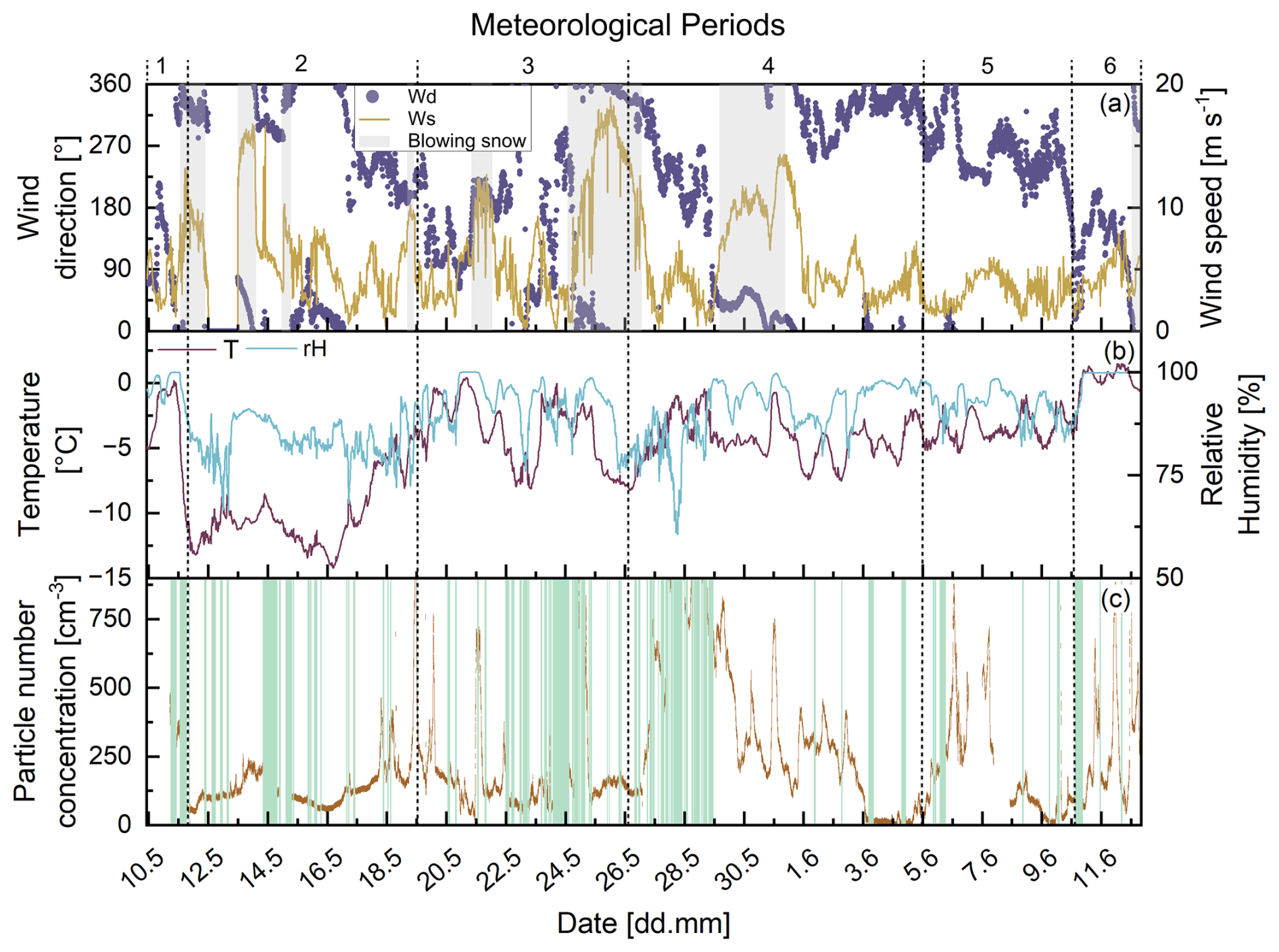
Figure 5 Overview of the six periods (dashed lines) for the entire measurement period, from 10 May to 12 June 2023, with (a) wind direction (W_d, purple, in °) on the left y axis. Meteorological data are shown as 10 min averages. The high wind speed events are shown in grey. Panel (b) shows the temperature (T, brown, in °C) on the left axis and the relative humidity (RH, blue, in %) on the right axis. Panel (c) shows the particle number concentration (cm⁻³), with pollution periods marked in turquoise.

3 Results and discussion

3.1 General overview

Based on radiosonde data, wind direction, and wind speed (Murto et al., 2024a, b), the expedition can be divided into six periods. For the first one and a half days, up until the morning of 11 May (Fig. 1), it was mild and moist, with temperatures around −2 °C and winds blowing from the southeast (Fig. 5a and b). Period 2, until 19 May, was characterized by low temperatures down to −14 °C and northwesterly/northeasterly winds. Period 3, until 26 May, was mild and moist again. The first temporary warming occurred on 20 May, when temperatures rose above 0 °C and southerly winds predominated. In Period 4 until 5 June, northerly winds predominated, accompanied by fluctuating temperature and humidity. Period 5, until 10 June, had temperatures near the melting point again, with warm, dry air aloft and westerly winds. Persistent melt onset occurred on 10 June in the early morning around 06:00 UTC, at the start of period 6, accompanied by rain and southerly winds. In total, eight high wind speed events with durations of at least 4 h were identified during the campaign. These events had wind speeds sufficiently high that blowing snow could potentially occur. Blowing snow cannot be described by a single fixed wind speed threshold (Fig. A2), as the threshold varies with temperature and snow properties. Warmer snow increases cohesion, while very cold snow increases friction, both leading to higher threshold wind speeds (Li and Pomeroy, 1997). Therefore, a critical threshold derived from air temperature and wind speed using an empirical model was calculated (Li and Pomeroy, 1997). These periods are indicated by grey shading in Fig. 5a. The longest continuous high wind speed event occurred between 24 and 26 May, during which wind speeds reached 19 m s⁻¹ (10 min average).

After excluding pollution periods, the average particle concentration for the entire period from 10 May to 12 June 2023 is 220 cm⁻³. Days with particularly high concentrations were 27 to 29 May, when the daily average was between 500 and 750 cm⁻³ (Fig. 5c). Conversely, periods with particularly low concentrations were 15 May and 3 and 4 June, with daily averages between 20 and 80 cm⁻³. The particle size distribution indicates a characteristic transition from Arctic haze to less polluted conditions in late May. Before 26 May, there is a pronounced accumulation mode, with particle concentrations peaking at diameters around 110 nm. This is subsequently replaced by a dominant Aitken mode, with a maximum concentration near a diameter of 50 nm. Also, events of high wind speed on 13 May, 24 to 26 May, and 31 May coincide with elevated particle number concentrations. Strong winds can enhance sea salt aerosol production through processes such as sea spray and sublimation of blowing snow (Heutte et al., 2025; Ranjithkumar et al., 2025). However, increased concentrations may also reflect transport of marine aerosol from open water (Lapere et al., 2024). The higher concentrations on 12 June could be linked to the onset of melting, as melt-related surface changes have been suggested to enhance aerosol production in the High Arctic (e.g., Mirrielees et al., 2024; Pereira Freitas et al., 2025). Low particle concentrations occurred during periods 2 and 4, which were characterized by lower temperatures (especially during period 2) and northerly winds. Air masses from the northern Arctic often contained relatively few aerosol particles due to the scarcity of local sources over the pack ice and deposition losses during transport.

The hourly surface type distribution based on the camera images over the full measurement period (Fig. 6a) shows that closed ice was most common at the beginning of the campaign and during the second ice camp from 29 May to 11 June. In contrast, during the first ice camp from 16 to 21 May, surface conditions varied more strongly, with mixed or rapidly alternating types. Overall, closed ice dominates on roughly two-thirds of the 34 measurement days. This high proportion is partly related to the ice camps (shaded in beige in Fig. 6d), during which Oden was typically surrounded by closed ice, resulting in a stronger influence of closed ice conditions, although open water was occasionally present.

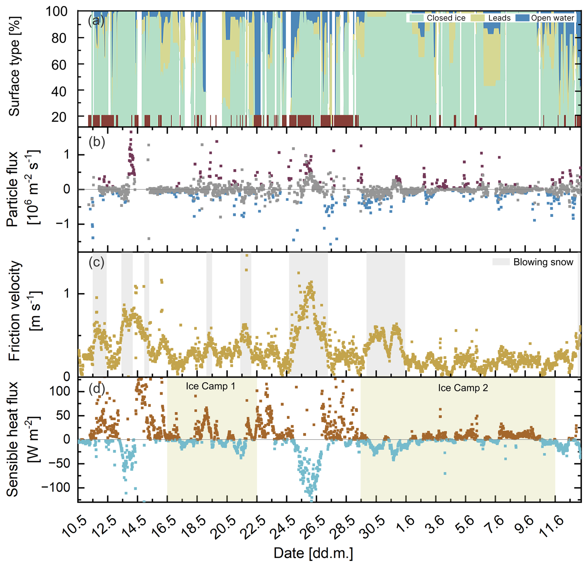
Figure 6 Overview of the surface types, particle and sensible heat fluxes, as well as the friction velocity for the entire measurement period, from 10 May to 12 June 2023. The top panel (a) shows the hourly distribution of the three surface types: closed ice (turquoise), leads (beige), and open water (blue). Periods with ship speeds ≥ 1 kn are indicated in red. The second panel (b) shows the particle flux (in 10⁶ m⁻² s⁻¹) evaluated in 20 min intervals (red squares indicate net particle emission, blue squares indicate net particle deposition, and grey squares indicate fluxes when 95 % confidence intervals include zero). The third panel (c) shows the friction velocity (u_*, in m s⁻¹) in beige, and the high wind speed events are shown in grey. The bottom panel (d) shows the sensible heat flux (W m⁻²) evaluated in 20 min intervals and the periods of the two ice camps (beige shading).

Over the entire expedition, the median 20 min net particle flux was −0.02 (interquartile range, IQR: −0.09 to 0.05) × 10⁶ m⁻² s⁻¹ (Fig. 6b). This overall net deposition results from a slightly larger proportion of net deposition intervals (58 % of 20 min intervals). Among the 20 min intervals with particle fluxes significantly different from zero at the 95 % confidence level, 53 % showed net deposition. Long, strongly pronounced continuous emission periods occur, for example, on 13 and 25 May, with median particle fluxes of 0.76 (IQR 0.46 to 0.97) × 10⁶ m⁻² s⁻¹ and 0.48 (IQR 0.18 to 0.53) × 10⁶ m⁻² s⁻¹, respectively. For extended net deposition, an example is the period from 29 to 31 May, with a median net particle flux of −0.14 (IQR −0.24 to −0.06) × 10⁶ m⁻² s⁻¹. When comparing emission- and deposition-dominated periods, no systematic differences in particle size distributions were observed between net positive and net negative flux periods. The median geometric mean diameter was 79.6 and 78.0 nm for net positive and net negative fluxes, respectively.

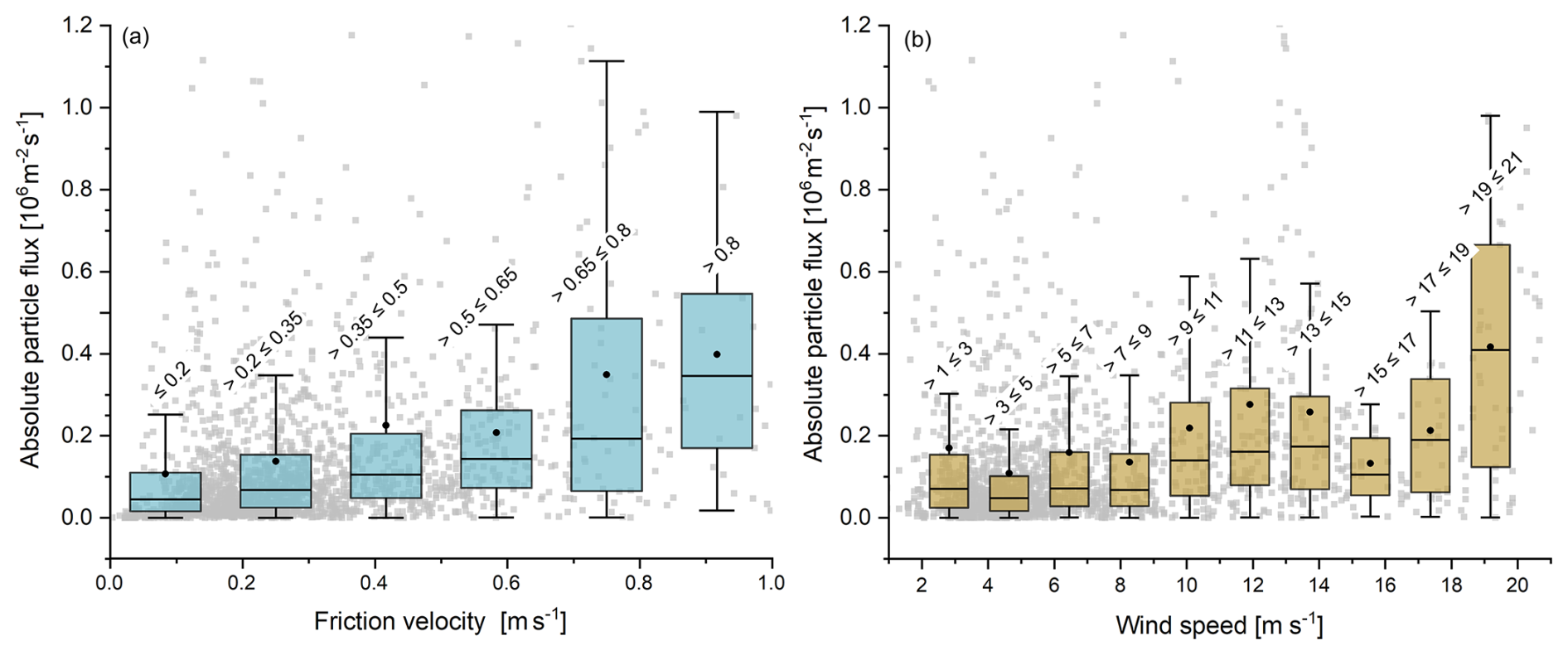
Figure 7 (a) Relationship between friction velocity (m s⁻¹) in different size bins and absolute net particle flux (in 10⁶ m⁻² s⁻¹). (b) Relationship between wind speed (m s⁻¹) in different size bins and absolute net particle flux (in 10⁶ m⁻² s⁻¹). The grey squares represent the individual 20 min values plotted against the corresponding friction velocity or wind speed on the x axis. The boxplots summarize these values within the bins indicated by the labels above each box. The boxes represent the 25th to 75th percentiles, while the whiskers indicate 1.5 times the interquartile range. The horizontal line denotes the median, and the black square represents the mean.

Previous studies have shown that the strength and direction of the sensible heat flux (Fig. 6d) are closely related to the surface type. Low or negative fluxes are typically observed over closed ice, whereas higher positive fluxes occur over open water (e.g., Held et al., 2011b; Mathes et al., 2025; Simon et al., 2025). The increased upward fluxes can be explained by the temperature gradient between the relatively warm water surface (close to the freezing point) and the colder air above. In contrast, thick pack ice has a strong insulating effect, limiting heat exchange with the underlying ocean. Surface temperatures are therefore lower, and sensible heat fluxes are reduced (Held et al., 2011b). Figure 6a and d shows that enhanced upward sensible heat fluxes coincide with periods of leads and open water. Strongly negative sensible heat fluxes during high wind speed events suggest heat is being transferred from the atmosphere to the ice surface. This is likely associated with the advection of warmer air masses over the colder ice surface. Higher wind speeds enhance turbulent exchange, thereby increasing the flux. During these periods, turbulent heat fluxes largely control the energy exchange at the surface. On average, sensible heat fluxes are close to zero over the full annual cycle (Tjernström et al., 2012), indicating that they are not controlled by surface type alone but also by seasonal and atmospheric variability.

The net particle flux is strongly influenced by the intensity of turbulence, which is indicated by the friction velocity u_* (e.g., Grönholm et al., 2009; Donateo et al., 2023). The median value of u_* is 0.26 (IQR 0.17 to 0.40) m s⁻¹ across the entire campaign (Fig. 6c). Days of high absolute particle fluxes coincide with periods of particularly high friction velocities (Fig. 7a). A linear regression analysis of the centers of six friction velocity bins (u_*) and the net particle flux reveals a strong correlation, with an R value of 0.88 (Fig. 7a). The first bin covers $u_{*}\le \mathrm{0.2}$ m s⁻¹ and the last bin covers $u_{*}>\mathrm{0.8}$ m s⁻¹, while the remaining boundaries were evenly spaced in between, with a width of 0.15 m s⁻¹. The relationship between wind speed and net particle flux was analyzed in the same way. The absolute net particle fluxes within the wind speed bins are varying (Fig. 7b), and the linear regression using the bin centers yields a correlation coefficient of R=0.62. This suggests that higher wind speeds are generally associated with stronger particle fluxes, although the linear relationship is weaker than for friction velocity (more on this in Sect. 3.3).

The stability parameter $z/L$ shows that weakly unstable conditions ($\mathrm{-}\mathrm{0.2}<z/L<\mathrm{-}\mathrm{0.02}$) dominated the measurement campaign. These conditions occurred in 34 % of the 20 min flux intervals. A predominance of near-neutral conditions and a broad range of atmospheric stability regimes have also been observed during previous turbulence measurements in the Arctic (Grachev et al., 2005; Srivastava et al., 2024). Neutral conditions ($\mathrm{-}\mathrm{0.02}<\mathit{\zeta }<\mathrm{0.02}$) were also common and occurred in 30 % of the intervals. Weakly stable conditions ($\mathrm{0.02}<\mathit{\zeta }<\mathrm{0.2}$) were much less common, occurring in 19 % of the intervals. There was no clear correlation between the observed particle fluxes and atmospheric stability conditions.

3.2 Particle fluxes – dependence on surface type

3.2.1 Measured particle fluxes

On 23 out of 34 measurement days, the particle flux measurements were primarily influenced by closed ice. On five other days, half of the surface was covered with closed ice. Previous studies have shown that the net particle flux over closed ice surfaces is often directed to the surface, indicating that closed ice surfaces act as particle sinks (e.g., Held et al., 2011a; Donateo et al., 2023). Taking into account all intervals in which closed ice covers more than 70 % of the surface, the median net particle flux is −0.02 (IQR −0.10 to 0.04) × 10⁶ m⁻² s⁻¹. From 29 May to 2 June, Oden was mostly surrounded by closed ice during the second ice camp (Fig. 6a). During this time, the particle flux was dominated by net deposition, except on 31 May (Fig. 6b). Comparing the net particle fluxes over closed ice with other studies over the same surface type shows that they span a wide range of magnitudes (Fig. 8). For instance, fluxes ranging from −0.08 to 0.05×10⁶ m⁻² s⁻¹ were observed at closed ice surfaces in the Arctic using the eddy covariance method (Nilsson and Rannik, 2001; Held et al., 2011a; Donateo et al., 2023). Net particle fluxes using the gradient method are −0.16 to 0.12×10⁶ m⁻² s⁻¹ (Held et al., 2011b; Mathes et al., 2025). In Antarctica, median fluxes ranged from −3.33 to 2.75×10⁶ m⁻² s⁻¹ (Grönlund et al., 2002). Direct comparisons of flux magnitudes between studies should be made with caution. Strong fluxes often represent individual (e.g., a single 20 min averaging period) measurements. When averaging or calculating medians, positive and negative fluxes tend to cancel each other out, resulting in values closer to zero.

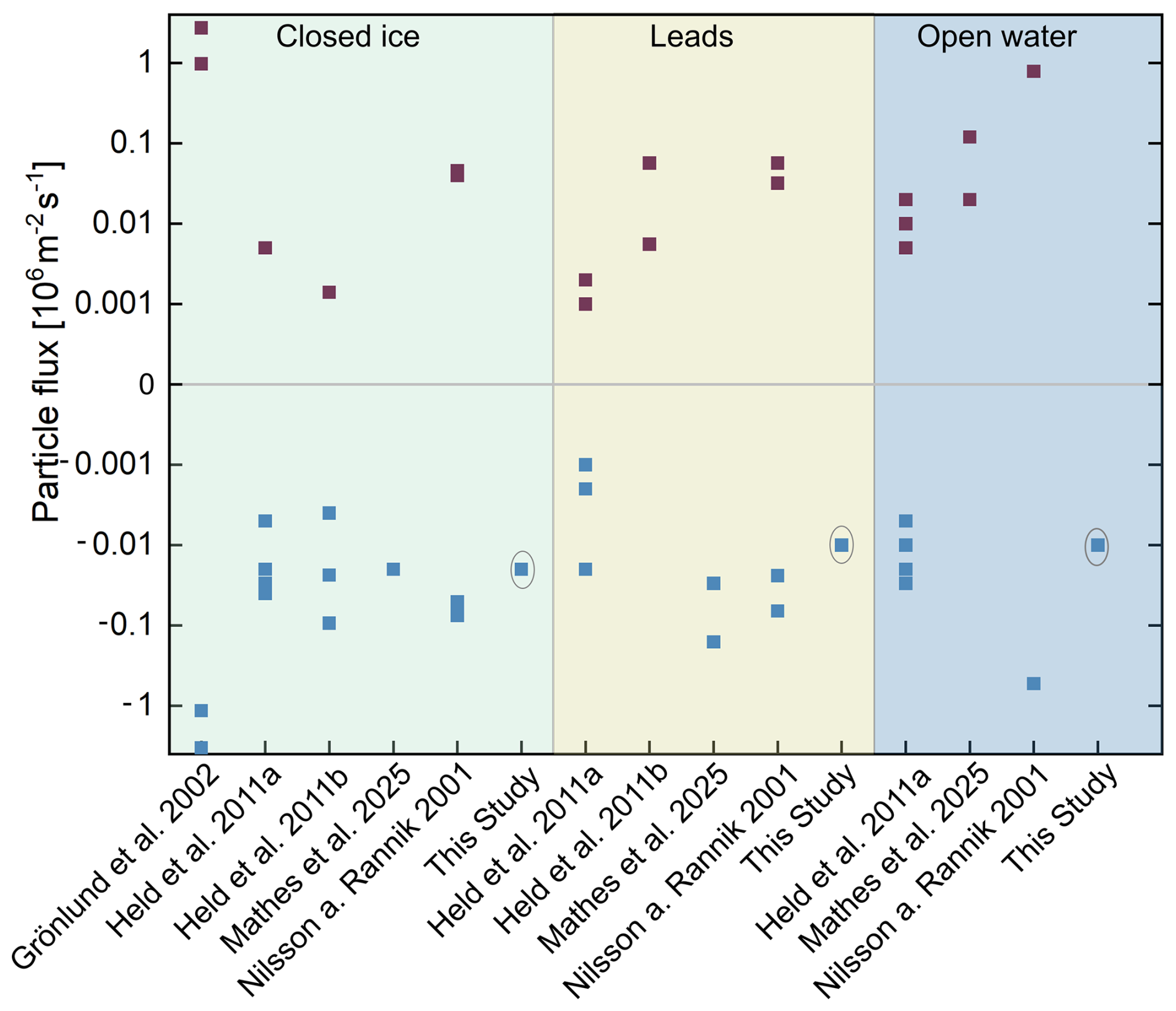
Figure 8 Overview of particle fluxes (10⁶ m⁻² s⁻¹) of this study and comparable studies, depending on the surface type. Positive fluxes indicate net emission (red), whereas negative fluxes indicate net deposition (blue). The three background colors indicate the surface types closed ice, leads, and open water. For this study, the grey circles indicate the median particle flux for each surface type. Multiple values shown for previous studies correspond to values reported by the respective authors (e.g., different measurement sites, periods, or statistics).

Existing literature makes little distinction between open water, wide, and narrow leads. As the flux footprint may extend beyond the lead, the effective footprint depends on the lead width, limiting the attribution to one specific surface type. Various explanations have been proposed for the formation of particles in connection with leads. Bubble bursting has been observed at wind speeds of around 4 m s⁻¹ and above (May et al., 2016; Kirpes et al., 2019). However, Held et al. (2011a) demonstrated that measurable particle emission fluxes can also occur at low wind speeds. This suggests that emissions from leads and open water are not exclusively driven by wind. The formation of marine aerosols without wind influence has been well documented, including in the High Arctic (Leck et al., 2002). Bubble formation can also occur independently of wind speed. Possible mechanisms include the nucleation of microbubbles at low supersaturation levels, their stabilization by surfactants, and the formation of subsurface bubble layers that can be detected acoustically. These processes can result in bubbles bursting more slowly at the interface between air and sea. Freezing and melting processes, and the release of biogenic gases, may further support these mechanisms (Mulhearn, 1981; Johnson and Wangersky, 1987). This is consistent with earlier reports of aerosol emission over open leads without visible bubble activity (Scott and Levin, 1972). It is also in agreement with observations of bubbles in the surface waters of leads occurring under weak wind conditions and thin ice cover (Norris et al., 2011). In the open ocean, wind-driven breaking waves typically produce bubble clouds that extend a few meters below the surface (e.g., Anguelova and Huq, 2012). These conditions also promote the selective uptake of high molecular weight organic matter into sea spray droplets (Farmer et al., 1993). Whitecaps in pack ice regions tend to be smaller and occur less frequently than in the open ocean. This may explain the comparatively weak net emission observed over leads and open water during this campaign, where the median particle flux is close to zero. This suggests that, although such emission events are possible, they do not dominate the overall particle exchange between the surface and the atmosphere.

Quantitatively, the magnitude and sign of the fluxes observed in this study are in good agreement with earlier measurements. Held et al. (2011a) reported an almost equal number of net emission and deposition events associated with open water. The observed fluxes ranged from −0.03×10⁶ to 0.02×10⁶ m⁻² s⁻¹ (Fig. 8). These closely match the near zero median fluxes obtained here. Both positive and negative fluxes over open sea were also observed by Nilsson and Rannik (2001). The median value of positive fluxes above open water was 0.79×10⁶ m⁻² s⁻¹, while the median value of negative fluxes was −0.53×10⁶ m⁻² s⁻¹ (Nilsson and Rannik, 2001).

For narrow leads, Held et al. (2011a) reported fluxes in a similar range from −0.02×10⁶ m⁻² s⁻¹ to slightly positive values using the eddy covariance method. In contrast, fluxes determined using the gradient method were all positive but limited to a few selected periods (Held et al., 2011b). The flux reported by Nilsson and Rannik (2001) for leads ranged from −0.07 to 0.06×10⁶ m⁻² s⁻¹ (Fig. 8). When both positive and negative fluxes are considered, the net flux is found to be close to zero (Nilsson and Rannik, 2001). However, as each value represents the net flux, this does not imply an absence of emissions, but rather that emission and deposition events balance each other out. This is consistent with the dominance of weak deposition or median flux values close to zero observed in this campaign. May et al. (2016) and Willis et al. (2018) state that the strongest net emission particle fluxes occur most frequently in the vicinity of seawater, although fluxes from leads are an order of magnitude lower than those over the open ocean. Model simulations suggest that leads contribute between 0.3 % and 3 % to the annual locally emitted sea salt particle flux (Lapere et al., 2024).

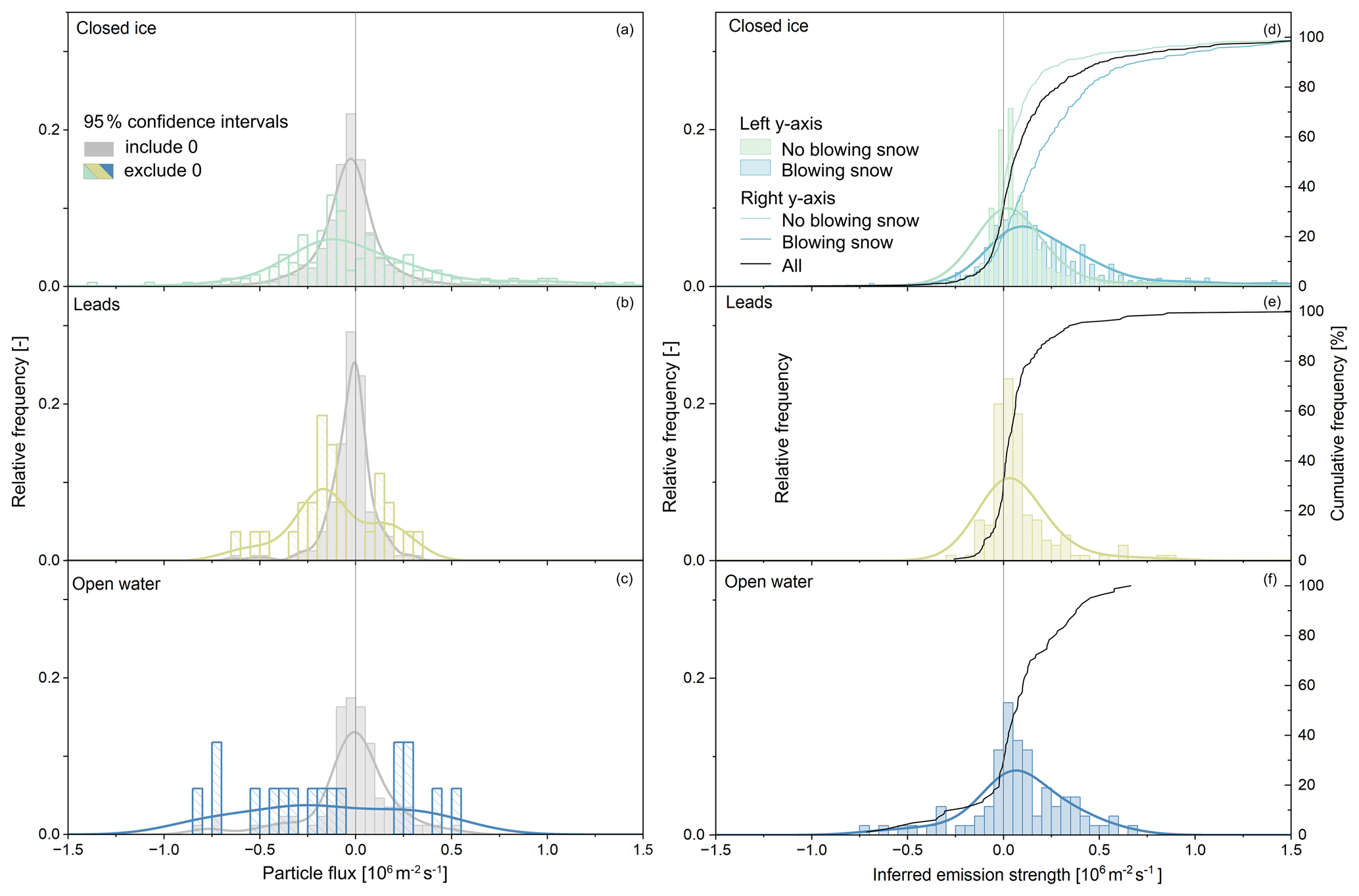
Figure 9 The left panels (a)–(c) show the relative frequency distributions of particle number fluxes (in 10⁶ m⁻² s⁻¹) for the three surface types: (a) closed ice, (b) leads, and (c) open water. Colored bars represent fluxes when 95 % confidence intervals exclude zero, whereas grey bars represent fluxes when 95 % confidence intervals include zero. The vertical grey line indicates zero flux, separating net particle deposition from net particle emission. Only stationary periods with ship speed ≤ 1 kn are included. The bold curves show the kernel density estimation. The right panels (d)–(f) show relative and cumulative frequency distributions of inferred emission strength (in 10⁶ m⁻² s⁻¹) for the three surface types: (d) closed ice, (e) leads, and (f) open water. The distributions are derived from observed particle fluxes and modeled deposition velocities, shown separately for periods without potential blowing snow (green) and with potential blowing snow (blue), depending on the blowing snow threshold. For closed ice (d), distributions are shown separately for periods without potential blowing snow (green) and with potential blowing snow (blue). The bold curves show the kernel density estimation. The left y axis (histograms) shows the relative frequency, while the right y axis shows the cumulative frequency distributions for no potential blowing snow (green line), potential blowing snow (blue line), and all observations (black line).

The relative frequency distribution of particle number fluxes over closed ice (Fig. 9a) shows that the particle flux is dominated by deposition, accounting for about 70 % of all intervals. The largest contribution (approximately 22 %) is associated with weak deposition, with fluxes between 0 and −0.025×10⁶ m⁻² s⁻¹. For intervals during which leads were the dominant surface type (>50 % of the classified surface area, approximately 7 % of the total measurement period), net deposition was dominant, with a median flux of −0.01 (IQR −0.10 to 0.08) × 10⁶ m⁻² s⁻¹ (Fig. 9b). For intervals in which open water was the dominant surface type (>50 % of the classified surface area, approximately 5 % of the total measurement period), the median net particle flux was −0.01 (IQR −0.09 to 0.05) × 10⁶ m⁻² s⁻¹. Positive and negative flux intervals occurred in nearly equal numbers (Fig. 9c). This indicates that although open water surfaces can act as a particle source, their overall contribution to particle emission is limited during the campaign. A substantial fraction of open water periods was removed from the dataset, since Oden was typically underway when open water was present, and surface type evaluation was restricted to slow movement of the vessel. As a result, particle fluxes associated with open water are likely underrepresented in the filtered dataset. These results place the observed fluxes over leads and open water in a regime characterized by weak net exchange and substantial variability, a behavior that is consistent with previous studies. Comparing fluxes for which the 95 % confidence intervals exclude zero (colored bars) with fluxes for which the intervals include zero (grey bars) shows that the majority of fluxes close to zero fall into the latter group. The qualitative pattern is similar in both cases. Negative fluxes predominate over closed ice, while both positive and negative fluxes occur over leads and open water.

3.2.2 Inferred particle emission strength

The inferred emission strength is defined as the difference between the measured net particle flux and the modeled deposition flux. Figure 9d–f shows the relative and cumulative frequency distributions of the inferred emission strength categorized by surface type and by periods with and without potential blowing snow. Positive values indicate the estimated particle emission at the surface. Negative values result from a measured net flux more negative than the modeled deposition. These cases result from the natural scatter in both the measured net particle flux and the inputs to the deposition model, as well as from the uncertainty in the deposition model itself. In our study, negative inferred emission strengths occurred in 32 % of the evaluated measurement intervals. However, the median magnitude of these negative inferred emission strengths ($-\mathrm{0.05}\times {\mathrm{10}}^{\mathrm{6}}$ m⁻² s⁻¹) was smaller than the combined uncertainty (0.07×10⁶ m⁻² s⁻¹) of the sampling error following Finkelstein and Sims (2001) and the random uncertainty due to limited counting statistics according to Buzorius et al. (2003). Furthermore, 57 % of the negative inferred emission flux values were smaller than the combined uncertainty of the corresponding particle flux measurements. This indicates that most negative inferred emission fluxes are within the uncertainty of the particle flux measurements. In the absence of particle emission, the measured net particle flux is expected to approach the modeled deposition flux, resulting in inferred emission values that scatter around zero within the associated uncertainties. The predominance of small negative values is consistent with this expected behavior. For measured net emission fluxes, the inferred emission strength is always more positive than the measured flux, because the modeled deposition flux is negative by definition. Therefore, independent of uncertainty in the magnitude of the modeled deposition flux, a positive inferred emission strength is statistically significant when the 95 % confidence interval of the measured net emission flux does not cross zero. This criterion was met in 29 % of intervals with measured net emissions.

Over closed ice (Fig. 9d), high wind speed conditions are associated with a shift in inferred emission strength towards higher values. During periods when the threshold for blowing snow was not exceeded, the distribution is centered around zero and dominated by weak inferred emission. In contrast, periods with high winds show a higher frequency of positive inferred emission. These results suggest stronger particle emission relative to deposition under high wind speed conditions. This behavior is also reflected in the cumulative frequency distributions. Together, the results in Fig. 9d demonstrate that high wind speed conditions are primarily associated with enhanced inferred particle emission over closed ice. For leads (Fig. 9e), only a small number of intervals meet the blowing snow threshold. This reflects limited sampling during high wind speed conditions, as measurements during storm events were predominantly conducted over closed ice. Consequently, few high wind cases are available for leads, and the effect of blowing snow on inferred emission strength cannot be robustly assessed. For open water (Fig. 9f), blowing snow is not relevant, and none of the intervals exceed the blowing snow threshold.

3.3 Net particle emission during high wind speed events

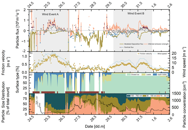
In total, eight events of high wind speed with a potential for blowing snow were identified during the campaign (see Sect. 3.1). Due to the faster mobilization of cold, dry snow, the blowing snow threshold would at times already be reached at wind speeds of 6 m s⁻¹ at low temperatures (Fig. A2). Five of the eight events are characterized by net particle emission. One shows flux values close to zero, and two are dominated by net deposition. Most of the events of high wind speed occurred when the prevailing surface type was closed ice. Across all eight events, the median friction velocity ranged from 0.45 to 0.69 m s⁻¹, reflecting consistently enhanced turbulence during conditions favorable for blowing snow. Two emission dominated high wind speed events, on 24–26 and 29–31 May, are highlighted in Fig. 10 as they exhibit strong and persistent particle emission fluxes. Event A (24–26 May) is characterized by strong net emission fluxes of up to 0.98×10⁶ m⁻² s⁻¹ (95 % confidence interval excluding zero) and by being the longest continuous net emission period of the entire measurement campaign (Fig. 10a). The inferred emission strength reached a maximum value of 1.2×10⁶ m⁻² s⁻¹. Figure 10b further shows that the strongest emission fluxes occur nearly simultaneously with peaks in friction velocity and wind speed. During this event, closed ice dominated the surface conditions (Fig. 10c), although individual hours were intermittently influenced by open water. Similarly, during the event from 29 to 31 May (Event B), closed ice remained the predominant surface type, and the inferred emission strength reached values up to 1.57×10⁶ m⁻² s⁻¹ (Fig. 10a). The coincidence of favorable conditions for blowing snow, enhanced turbulence, and net particle emission over predominantly closed ice suggests the presence of a wind related particle source. This is consistent with processes associated with blowing snow, which can temporarily outweigh the deposition fluxes typically observed over closed ice.

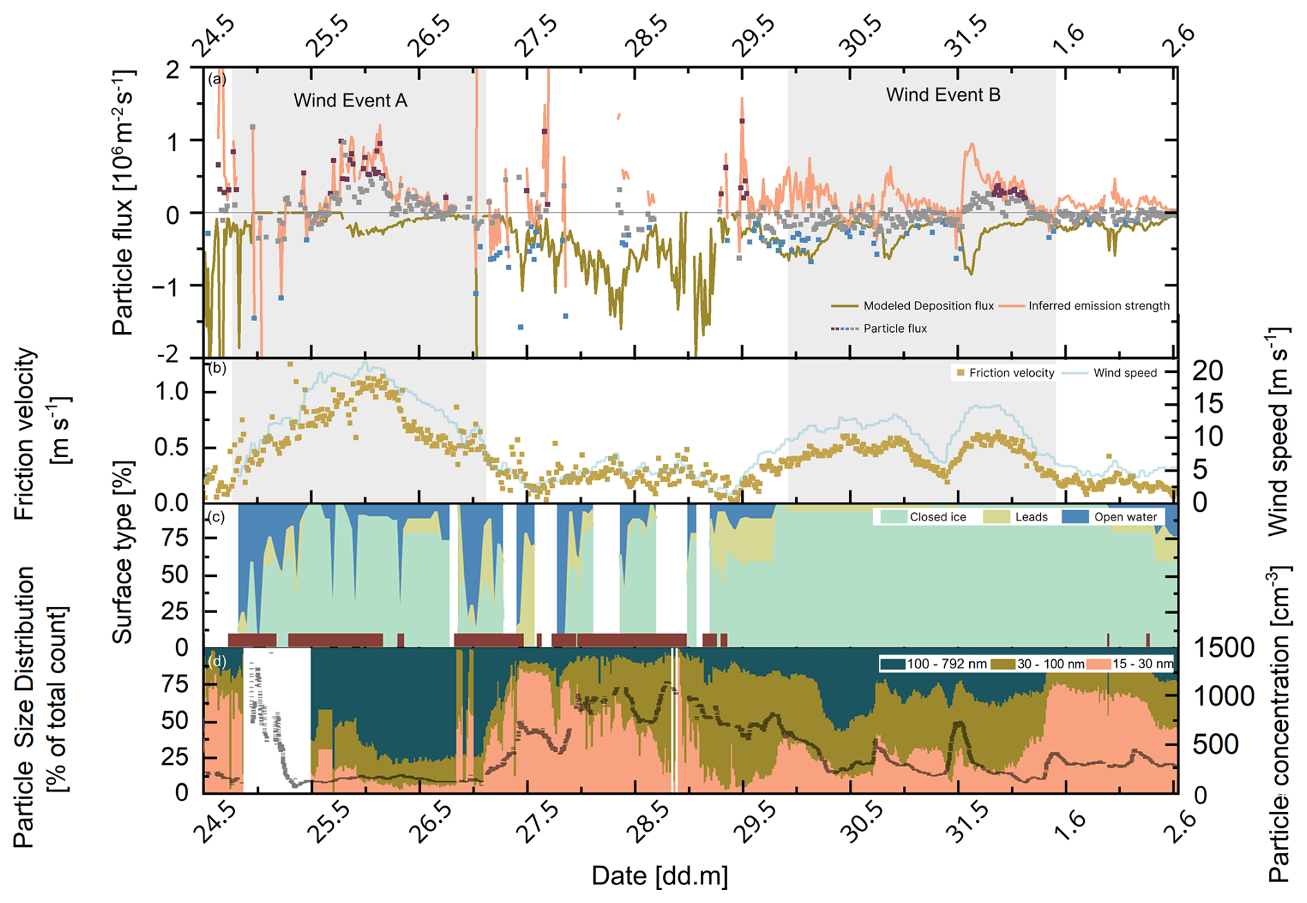
Figure 10 (a) Particle fluxes (red squares indicate net particle emission, blue squares indicate net particle deposition, and grey squares indicate fluxes when 95 % confidence intervals include zero), modeled deposition flux (dark beige), and inferred emission strength (salmon-colored) from 24 May to 2 June evaluated in 20 min intervals (in 10⁶ m⁻² s⁻¹). Panel (b) shows the friction velocity (u_*, beige, in m s⁻¹) and wind speed (light blue, in m s⁻¹). The grey shading in (a, b) shows the time periods when the threshold for blowing snow is exceeded. Panel (c) shows the hourly distribution of the three surface types: closed ice (turquoise), leads (beige), and open water (blue). Periods with ship speeds ≥ 1 kn are indicated in red. (d) Particle size fractions from 15 to 792 nm in three accumulated groups (left y axis, in % of total particle number concentration) measured with a DMPS on the fourth deck of Oden and total particle number concentration (cm⁻³), measured with an MCPC at the foremast (black symbols; right y axis).

One type of particles associated with high wind speeds above sea ice is sea salt aerosol (SSA), which spans particle sizes from submicron to coarse ranges and can be produced by the sublimation of blowing snow. While the open ocean is the largest source of SSA, with wave breaking and bubble bursting generating film and jet drops (e.g., de Leeuw et al., 2011), several studies show that strong SSA sources are also associated with sea ice. Sublimation of salty blowing snow is considered a major source of SSA in sea ice dominated environments (Frey et al., 2020; Ranjithkumar et al., 2025). In addition to particles measured in coarse mode (Yang et al., 2019; Frey et al., 2020; Ranjithkumar et al., 2025), Gong et al. (2023) observed an increase in particles ranging from 10 to 300 nm during blowing snow events. The evolution of the particle size distribution in Fig. 10d shows that particles between 100 and 300 nm were dominant during Event A. During Event B, enhanced concentrations were mainly observed between diameters of approximately 30 and 100 nm, while no distinct nucleation mode was evident. This is consistent with elevated particle concentrations below 300 nm as observed by Gong et al. (2023). Therefore, one likely explanation for the observed net particle emissions during Events A and B is that particles were generated by the sublimation of blowing snow during the high wind speed events. This production outweighs the deposition processes occurring simultaneously on closed ice surfaces. This is also evident in the results of the deposition model (Fig. 10a), which shows an increased inferred emission strength. Furthermore, it becomes clear from Fig. 10a that at the onset of Event B, the particle emissions caused by blowing snow are masked by deposition fluxes, so that there is no net emission but deposition at the beginning of this event. Measurements of particle fluxes taken on the ice during the same campaign using the gradient method also indicate emission fluxes associated with blowing snow (Mathes et al., 2025). An alternative source of the observed particles could be sea spray aerosol generated from leads or open water (Kirpes et al., 2019; Dall'Osto et al., 2026). The classification as closed ice indicates that closed ice accounted for at least 70 % of the surface within the selected area. Therefore, small fractions of leads or open water may have been present during some intervals, and a contribution from sea spray aerosol cannot be completely excluded. However, the predominance of closed ice and the coincidence of positive particle fluxes with blowing snow conditions suggest that sea spray aerosol was unlikely to be the main source. New particle formation is also considered unlikely to explain the observed positive particle fluxes. This process requires precursor gases and oxidants, and particle formation may occur within or above the atmospheric boundary layer rather than directly at the surface (Burkart et al., 2017; Simon et al., 2025). Newly formed particles would therefore not necessarily produce an upward particle flux originating within the flux footprint. Furthermore, the measured particle size distributions during Events A and B did not exhibit a distinct nucleation and growth pattern. Instead, elevated particle concentrations were observed across a broad size range, supporting the interpretation that blowing snow was the more likely source of the observed particle emissions (Gong et al., 2023; Ranjithkumar et al., 2025).

Previous modeling studies have often assumed that blowing snow particles consist solely of sea salt (Chen et al., 2022). However, this assumption ignores the chemical complexity of Arctic snow, which has been shown to contain organic matter, as well as nitrate and sulphate (Grannas et al., 2007; Macdonald et al., 2018; Mori et al., 2019). Studies demonstrate that blowing snow events are associated with increased sulphate concentrations (Gong et al., 2023) as well as elevated submicron sodium and chloride masses (Chen et al., 2022). Observations from the ARTofMELT campaign further demonstrate that Arctic snow contains amounts of organic and biological material, and black carbon. They highlight that blowing snow particles cannot be assumed to consist of sea salt alone (Pereira Freitas et al., 2025).

4 Summary and conclusions

During the ARTofMELT campaign, turbulent particle fluxes in the High Arctic were successfully determined using a continuous five week eddy covariance dataset. The measurements were conducted under a variety of meteorological and surface conditions. The results provide insight into the surface dependent variability of particle exchange processes over closed ice, leads, and open water, in a region undergoing rapid climate change.

Throughout the campaign, periods of net particle emission and periods of net particle deposition were observed, with deposition slightly predominating (58 % of all 20 min flux intervals). Among the intervals when 95 % confidence intervals excluded zero, 53 % showed net deposition. Median net deposition fluxes of −0.02 (IQR −0.10 to 0.04) × 10⁶ m⁻² s⁻¹ over closed ice confirm that this surface type generally acts as a particle sink under low to moderately turbulent conditions. However, net particle emission fluxes over closed ice were observed during periods of strong winds and increased turbulence with friction velocities $u_{*}>\mathrm{0.45}$ m s⁻¹. Under such conditions, the mobilization and sublimation of blowing snow can act as a source of particles in the atmosphere. The resulting net emission fluxes reached 0.98×10⁶ m⁻² s⁻¹ (95 % confidence interval excluding zero), much higher than the net deposition fluxes. These strong particle emission events were accompanied by an increase in total particle concentration, suggesting that particle emissions from blowing snow can temporarily dominate the local aerosol budget and mask the deposition typically observed over ice surfaces. This interpretation is supported by the comparison of measured net particle fluxes with modeled deposition fluxes, which reveals enhanced inferred emission during high wind speed events over closed ice. The magnitude of these inferred emissions remains subject to substantial deposition modeling errors. Net particle emission was also observed during periods influenced by open water. The magnitude and variability of these fluxes suggest that open water can act as a particle source, however, at times too weak to outweigh particle deposition. Similarly, leads exhibited deposition and emission events, with median fluxes close to zero. This reflects their dual role as both a particle source and a particle sink.

Our results demonstrate that surface heterogeneity has a strong influence on turbulent particle fluxes in the High Arctic. The emission fluxes observed in this study, and their contribution to local particle concentrations, suggest that particle emissions from leads could impact the microphysics of Arctic clouds under suitable meteorological conditions. However, this influence has yet to be quantified. Climate models predict continued sea ice loss and a corresponding increase in open water areas (IPCC, 2023). Changes in the frequency and intensity of particle exchange processes associated with sea ice are expected. Such changes may influence the background aerosol population and thereby affect concentrations of particles relevant to cloud formation and cloud properties. However, the net effect remains poorly constrained and depends on competing source and sink processes.

The overall climatic effects of changing particle and CCN number concentrations in the Arctic, whether cooling due to increased cloud albedo or warming due to changes in cloud lifetime and phase, remain uncertain (e.g., Cox et al., 2015; Schmale et al., 2021; Tan et al., 2023). In summary, this study has improved our understanding of the interactions between particles, surfaces, and the atmosphere in the Arctic. The quantitative characterization of particle deposition on closed ice and particle emissions from leads can help to better constrain and reduce uncertainties in model simulations of Arctic aerosol–cloud–climate interactions.

Appendix A

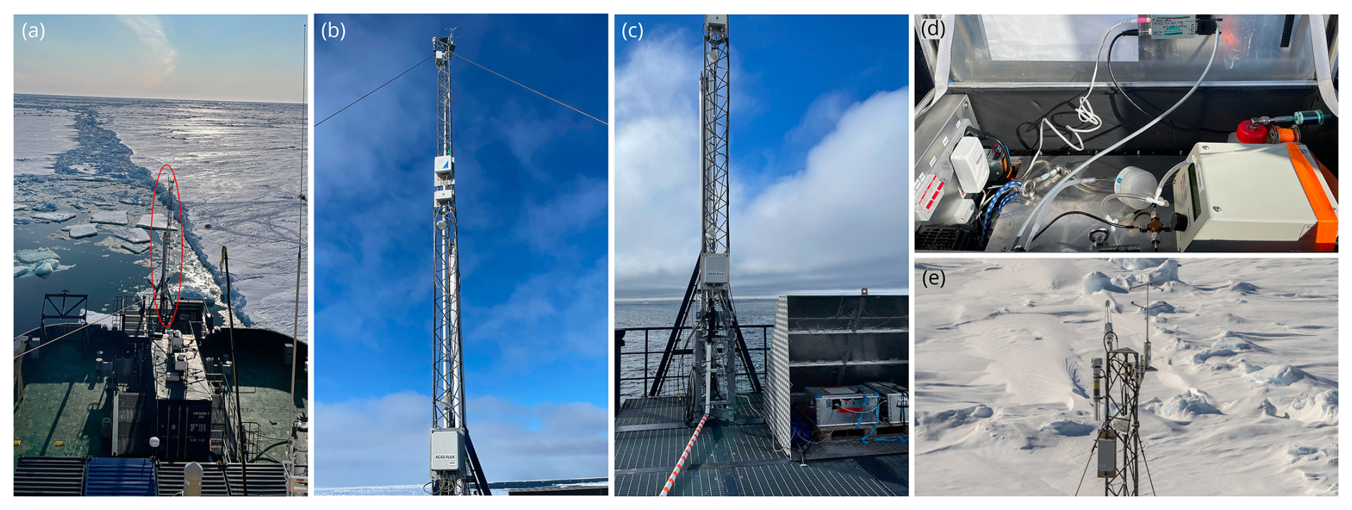
Figure A1 Pictures of the eddy covariance instrumentation installed on the foremast of Oden. (a) Forward looking view of the foredeck illustrating the position of the foremast at the bow of the ship (the red circle shows the foremast). (b) View of the foremast showing the sonic anemometer mounted at the top of the mast. (c) View of the lower part of the foremast with the aluminium housing containing the MCPC installed at the base of the mast. (d) MCPC with bypass system in the aluminium housing. (e) View of the top of the foremast with the sonic anemometer (Image credit Michael Tjernström).

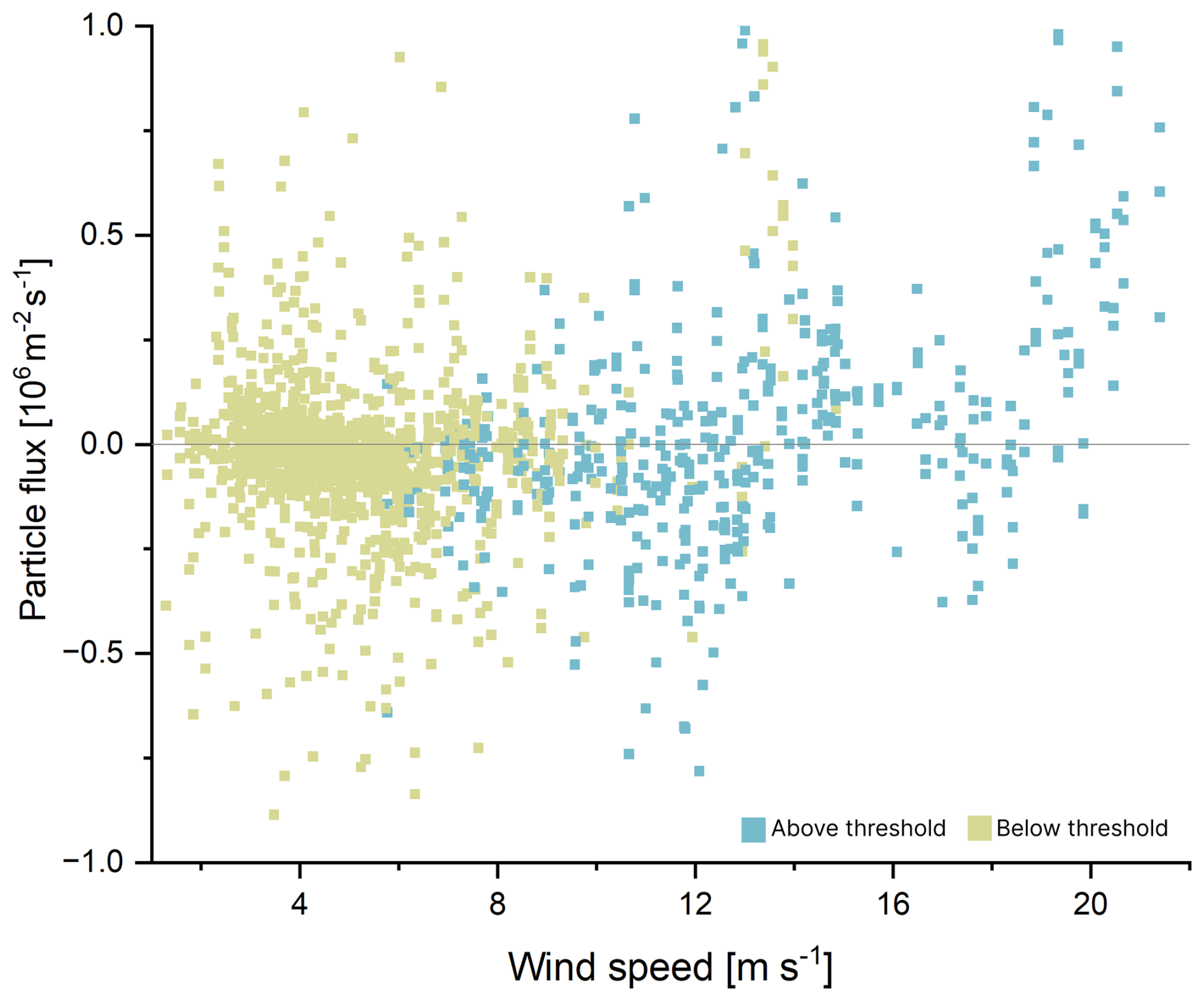
Figure A2 Net particle flux (in 10⁶ m⁻² s⁻¹) for closed ice as a function of wind speed (in m s⁻¹). Colors indicate whether the blowing snow threshold is exceeded (beige: below threshold, turquoise: above threshold), highlighting the conditions under which snow transport is initiated.

(Mathes et al., 2025)(Mathes et al., 2025)(ESDU, 1972)(Zhang et al., 2001)(Emerson et al., 2020)(Emerson et al., 2020)

Table A1 Parameters and constants used for the calculation of size-resolved dry deposition velocities following Zhang et al. (2001), with modifications after Emerson et al. (2020).