Influence of irradiance and mixing layer height on the vertical trace matter distribution in the lower planetary boundary layer – drone-based investigation

Drone-based atmospheric measurements allow time-resolved investigation of stratification in the lower atmosphere of many atmospherically relevant variables. Measuring a variety of variables can be used, e.g., for mixing layer (height, MLH) identification and examination of the representativity of ground-based measurements in the lowermost boundary layer. We present drone-based vertical profiling during two 2.5-week summer field campaigns in rural Germany to investigate the vertical distribution of trace matter and meteorological variables in the lowermost troposphere.

Night-time vertical profiling of temperature, humidity, wind speed, and trace substances (CO₂, O₃, particle mass and number concentrations) in the lowest 120 m revealed a multiple-layer fine-scale stratification. Trace substances surpassed several traditional meteorological variables in sensitivity for MLH detection. Among all variables, O₃ and potential temperature were the most reliable MLH markers, highlighting combining trace matter and meteorological measurements to understand stratification processes.

Using a gradient-based approach for diurnal vertical profiles up to 500 m above ground, we evaluate under which conditions and to which degree ground-based measurements, used world-wide in networks or during individual field campaigns, can be taken as representative for the lowermost mixing layer, and how strong radiative-driven mixing reduces vertical gradients. Location-specific sources and sinks affect the trace matter distribution in the ML much stronger than irradiance. However, homogeneity of aerosol particle concentrations was strongly promoted under high-radiative conditions, even at low MLHs. This suggests distinguishing between high- and low-irradiation conditions in the planetary boundary layer could improve parameterization for vertical mixing and should be considered when evaluating ground-based data.

1 Introduction

Ground-based measurements have been the primary method for ambient air quality research and monitoring, evolving from single-point observations to monitoring networks for various pollutants (EPA, 2025; UBA, 2025) and reference stations (Hoerger et al., 2015; Pastorello et al., 2020). It is typically assumed that measurements from a single station are representative for a broader area. The representativity of a measurement site is a vaguely defined quantity for how well a measurement station provides data that are not influenced by local anomalies (Hakuba et al., 2013; Merlone et al., 2024). Horizontally, representativity may range from only a few tens of meters for urban stations, but may reach over several hundreds of kilometers in flat, homogenous terrain (Ho et al., 2020; Yang et al., 2020). Vertical representativity is less critically reflected and is constrained by two considerations:

• a.

  It varies with horizontal location in complex terrain or in heterogeneous emission areas, where the vertical structure of air masses differs over short distances (Peters et al., 2022), and

• b.

  even over homogeneous terrain, the lower troposphere exhibits a pronounced diel stratification with diel changes in turbulence strength, limiting how well a near-surface measurement represents the boundary layer (Dandou et al., 2009).

Although these limitations are recognized – and (a) is typically considered during site selection, (b) is often neglected in ground-based studies, where the planetary boundary layer (PBL) is implicitly treated as uniformly “mixed.”

The mixing layer height (MLH) describes the upper boundary of a well-mixed lowermost layer, where chemically or dynamically different air masses adjoin. Reliably distinguishing the mixing layer from the adjacent layers is essential for the interpretation of microphysical and dynamical processes. The most-studied stratification in the lowermost troposphere is the PBL and free troposphere, at which boundary chemical, and thermodynamical different layers interface. We use the term “mixing layer” explicitly to describe a distinct atmospheric layer, independent on its location and time, i.e., a mixing layer can be the PBL or any shallow layer near ground. As MLHs differ throughout the times of day, and are affected by various mechanisms (e.g., formation of inversion layers, entrainment due to atmospheric instability Stull, 1988), definitions and diagnostic criteria that describe the upper boundary of the mixing layer are manifold and case dependent. Definitions range from changes of stability measures like the Richardson number and of the potential temperature gradient (Monin and Obukhov, 1954; Busch et al., 1976; Wyngaard and LeMone, 1980; Troen and Mahrt, 1986) to changes in the trace matter concentration profiles of, e.g., aerosol particles, O₃, or CO₂ (Collis and Ligda, 1964; Okada et al., 2012; Perrone and Romano, 2018; He et al., 2023). Some definitions are based on threshold values, other approaches consider gradient changes or inflection points in vertical profiles. Thus, a universal definition of the location of the upper boundary of the mixing layer and therefore the MLH does not exist (Mercer et al., 2018). Tan et al. (2025) characterized different PBLHs simultaneously and distinguished between a dynamical, thermal and material PBLH and attributed them to different atmospheric processes, which explains why different PBLHs coexist.

Available techniques for studying boundary layer meteorology include model approaches, experimental data, and hybrid methods. Regional-scale and re-analysis models provide insights into the vertical structure of the PBL (Nieuwstadt, 1984; Debolskiy et al., 2023), but model idealization may not reflect the influence of complex terrains like valleys or hills with complex dynamics and fail at predicting unusual stratification (Moeng and Sullivan, 1994; Emanuel and Živković-Rothman, 1999). Systematic variation of the MLH was even observed between different reanalysis tools (Julaha et al., 2025), showing the need of in-situ measurements. Ground-based measurements at different altitudes are often extrapolated to model vertical profiles (Monin and Obukhov, 1954; Troen and Mahrt, 1986). Remote-sensing tools like Lidars, radars and sodars provide low maintenance-intense altitude-resolved observations to support ground-based in-situ observations or to correct model data (Collaud Coen et al., 2014; Duncan Jr. et al., 2022; Kotthaus et al., 2023; Wang et al., 2025), though remote-sensing tools have an enhanced risk of misinterpretation due to the limited number of measurable variables. In situ platforms like balloons (Seidel et al., 2010; Valero et al., 2025), aircraft (Moores et al., 1979; Dai et al., 2014), tall towers (Andreae et al., 2015; He et al., 2023), and UAS (uncrewed aerial systems) can be used to record multiple variables for a comprehensive analysis (Reuder et al., 2012; McWilliams et al., 2023; Moormann et al., 2025), reducing uncertainty in boundary layer analysis. However, these methods are costly and labour-intensive (in construction and/or operation) and require extensive validation of the respective platforms. Weather balloons and aircraft rather focus on larger-scale phenomena, while towers and UAS typically operate within the lower few hundred meters above ground only. Towers require extensive installation, but can provide continuous long-term measurements, while UAS usually provide less data coverage but are flexible and manoeuvrable and therefore optimal for short-term boundary layer observations.

Recent studies used multi-platform approaches to improve UAS-based characterization of PBLs. UAS fleets have been applied to monitor atmospheric transport in a horizontal plane (Wetz et al., 2023), or vertical profiles to rule out temporal changes in the probed air masses (Borchers et al., 2025). Ground-based measurement stations have demonstrated to be not always useful as a reference (Barbieri et al., 2019), but can be used for spatial and temporal correction of UAS-based measurements for in-flight characterization of measurement instruments (Greene and Salesky, 2023; Moormann et al., 2025). For boundary layer studies, such multi-platform studies focused on, e.g., wind dynamics (Greene et al., 2022), altitude- and daytime-dependent aerosol composition within the PBL (Borchers et al., 2025), reconstruction of PBLs after the passage of rain fronts (Moormann et al., 2026), or the air pollutant distribution near civilization (Pohorsky et al., 2025). Furthermore, UAS can detect shallow layers near the ground by variables indicating dynamical, thermal and material mixing layer heights (Greene et al., 2022; Chilinski et al., 2024; Moormann et al., 2026).

Two fundamental assumptions for such studies are the representativity of UAS measurements within the PBL in general and the comparability of variables between UAS- and ground-based measurements. Greene et al. (2025) addressed the first assumption along with recommendations for sampling strategies, while this study focuses on the second one, using parallel UAS-based and ground-based in-situ measurements at two similar hilly rural sites in Central and Southern Germany during summer to evaluate

• a.

  the applicability and sensitivity of vertical profiles of various meteorological variables and trace matter (CO₂, O₃, and aerosol particle concentrations) for detecting fine scale vertical structures, including the mixing layer height, using gradient-based methods (up to 120 m altitude with 2 m vertical resolution) during a single nighttime event, featuring a fog event and a low-level jet,

• b.

  the dependence of aerosol gradients and atmospheric instability on irradiance and the PBL height (PBLH),

• c.

  the representativity of ground-based measurements with respect to the whole mixing layer (from vertical 500 m-profiling measurements) for meteorological variables and trace matter, focusing on influences from irradiance, the sampling site and standardization methods.

2 Methodology

Two field measurement campaigns (BISTUM23, August 2023 and BISTUM24, June 2024) were conducted at rural sites in Southern and Central Germany in summertime to investigate the influence of stratification on the trace matter distribution in the lowermost troposphere. For 2.5 weeks each, co-located UAS-based and ground-based measurements were performed.

2.1 Measurement sites

Both campaigns, BISTUM23 and BISTUM24, were conducted in rural grassy-forested areas in the German low-mountain ranges, with no strong nearby emission sources.

BISTUM23 took place near Albstadt, Swabian Alb (48°15^′ N, 8°59^′ E, Fig. S1 in the Supplement), with the ground station at 886 m above sea level from 3 until 17 August 2023. The site was chosen due to the absence of large habituated or industrialized regions upwind of the location.

BISTUM24 was performed near Spielberg, Vogelsberg region (50°19^′ N, 9°15^′ E, Fig. S1) with a ground station at 391 m a.s.l. from 7 until 22 June 2024. Air masses reaching the BISTUM24 site showed an anthropogenic influence indicated by enhanced pollution levels when they had passed the Frankfurt Rhine-Main metropolitan area (FRM, ∼ 30 km upwind with 5.9 million inhabitants). 24 h-backward trajectories (Sect. 2.2) with starting points in 50 m-altitude increments were used to differentiate between air masses that had passed FRM and air masses that had passed only rural regions prior to arriving at the BISTUM24 site. Using this classification, average vertical profiles of the trace substance variables O₃, CO₂ and the particle number concentration were calculated for both aspiration cases. Figure S2 shows that, although pollutant levels were higher when air masses had recently passed FRM, in both cases pollutants were well-mixed in the lowermost 500 m. Therefore, we consider the BISTUM24 site as sufficiently distant from major emission sources to be able to assume that anthropogenic plumes have already been vertically mixed.

Hence, we assume that the variability of trace matter concentrations in the lowermost 500 m for both campaigns and measurement sites are due to natural boundary layer dynamics and additional atmospheric processes and not driven by anthropogenic emissions.

2.2 Experimental data

During both campaigns, atmospheric data were collected using ground-based and UAS-based measurements. The ground-based aerosol research platform “MoLa” (Mobile Laboratory, Drewnick et al., 2012) operated continuously with inlets for aerosol and trace gases positioned 6 m above ground It was used for on-line measurement of various variables, including CO₂ and O₃ mixing ratios, particle number concentrations (PNC), particle mass concentrations across different size ranges, and meteorological data such as wind speed and direction, relative humidity, temperature, precipitation, and solar irradiance (Table S1). An ultrasonic 3D anemometer, positioned 5 m above ground near MoLa, was used to determine latent heat flux (Table S1; exclusively during BISTUM24).

The UAS-based measurement platform, known as the Flying Laboratory (FLab, Moormann et al., 2025), monitored a set of variables similar to several of those measured by MoLa. These included CO₂ and O₃ mixing ratios, PNC for particles larger than 10 nm (PNC_> 10 nm) and 350 nm (PNC_>350 nm), particulate matter PM₁ and PM_2.5, as well as meteorological data like horizontal wind speed and direction, temperature, and relative humidity (Table S1). The bulk Richardson number Ri, the potential temperature θ and equivalent potential temperature θ_eq were derived from the meteorological UAS data (Moormann et al., 2026).

While in MoLa, high-grade instrumentation was used for precise ground-based measurements, FLab utilized mid-grade sensors to minimize payload and enable aerial operation. FLab was typically operated hourly for vertical profiling up to 500 m above ground during the day, if rain or stormy gusts (> 16 m s⁻¹) did not threaten safe operation. In addition, one full-night operation for profiling the lowest 120 m was conducted during BISTUM24. Each flight lasted ∼15 min and began with hovering at 6 m above ground near the MoLa inlet for about one minute, followed by two ascents and descents with a vertical speed of 3 m s⁻¹. Between these ascents and after the final descent, additional hovering near the MoLa inlet was performed for comparison of the high-grade ground data with the UAS data.

2.3 Data Analysis

Instrumentation of MoLa and FLab were calibrated prior to the campaign. Regular inter-platform comparisons between MoLa and FLab (Sect. 2.2) were used to correct for sensitivity drifts of UAS-borne instruments as suggested in Moormann et al. (2025). The influences of rapid changes in humidity, temperature and pressure on the instruments during vertical motion were corrected with formulae provided by the respective manufacturers.

To account for temporal variation of advected air mass properties within the 15 min time frames of the individual flights, the FLab data were corrected using the ground-based measurements on-board MoLa. This approach neglects the altitude dependence of air mass transport properties (i.e., wind velocity and direction), based on the assumption that turbulent mixing levels out these influences to a certain degree and was applied in absence of the necessary measurement data, needed to account for such effects. Details on these corrections are explained in detail in Appendix A1. Data from UAS-borne measurements were averaged for vertical increments of 2 and 25 m for further investigation. Error calculations account for the standard error of the averages and the instrument's uncertainty for the respective averaging time (Moormann et al., 2025).

The PBLHs for both campaigns were estimated from the ICON-D2 model forecasts using the following criteria (Crueger et al., 2018; DWD, 2025): Brunt–Väisälä frequency > 5 × 10⁻⁵ s⁻¹, vertical gradient of potential virtual temperature > 0.3 K km⁻¹, and vertical gradient of absolute humidity must be curved. The setup and refining of the ICON-D2 model and the detailed PBLH estimation is methodically described in Moormann et al. (2026). The obtained model-based PBLH qualifies for comparison with trace substance and meteorological variables, as (a) dynamical, thermal and material PBLHs show a tight coupling in summer daytime under strongly convective conditions (Xin et al., 2026) and (b) thermal and material criteria were used in the model for the estimation of a single combined PBLH.

3 Case study: Height criteria and fine-scale structure of the nocturnal boundary layer

In the evening, the PBL transitions from convectively mixed daytime conditions to stable, stratified nocturnal conditions. This change results in a complex, time-dependent vertical structure of the boundary layer with several distinct layers (Nieuwstadt, 1984; Kotthaus et al., 2023). Various methods and modelling approaches are employed to determine nocturnal MLHs, similar to how MLHs are determined during the day. However, MLH detection methods that are based on a single atmospheric variable often fail unpredictably and independently of the daytime due to temporal changes in air mass dynamics or composition around the upper edge of the mixing layer or due to the lack of vertical resolution (Kotthaus et al., 2023). Remote sensing of various variables, revealed the simultaneous existence of different types of MLHs based on the variables referring to statical or dynamical stability and the vertical distribution of atmospheric constituents that identified stratification in a complex terrain with mountainous, urban and waterbody influences. Respective variables led to the definition of a dynamical, thermal and material boundary layer, respectively (Tan et al., 2025). This differentiation between those categories helps to explain atmospheric processes. While many MLH estimations rely on ground-based data, remote sensing and modelling approaches, methods based on frequent high-resolution in-situ measurements are considered the most accurate ones. These latter methods can typically determine MLHs with accuracies of a few meters (Cava et al., 2019; Mahrt and Acevedo, 2023).

To explore which are the most sensitive and most accurate atmospheric variables for determining MLHs during nighttime, we operated the FLab hourly throughout the night from 20 to 21 June 2024. Deriving the fine-structure of the NBL from different types of MLHs allows explaining atmospheric processes that cannot be identified otherwise. Vertical profiling commenced after the passing of a cold front (with associated heavy rain) at 15:00 (local summer time) on 20 June. During the night, the vertical profiling was legally limited to 120 m above ground, which was anticipated to be sufficiently high to surpass the nocturnal boundary layer (NBL) and eventually reach mixing layers aloft. While this limitation restricted the profiling flights to lower altitudes than in other measurements, it allowed to ascent/descent slower and more often. Longer sampling time in the 120 m range reduced data noise of the spatially highly-resolved hourly vertical profiles (2 m-increments in Fig. S3) helping to identify MLHs manually with a variety of FLab-measured trace substance concentrations (Fig. 1a) and meteorological variables (Fig. 1b) based on the observation of strong gradient changes and inflection points to address thermal and material MLHs, respectively. To account for subjectivity of this manual MLH-assignment approach, we estimated a conservative uncertainty based on the respective vertical profile (i.e., we estimated the range of justifiable MLHs for each case). Additionally to the gradient-based criteria, we use the bulk Richardson number (Ri) as a fixed criterion to identify the dynamical MLH due to its widespread use in boundary layer studies (Stull, 1988). Ri > 0.25 indicates dynamically stable atmospheric conditions (as expected inside the NBL due to the inversion and often weaker winds), while Ri< 0.25 describes unstable conditions (i.e., lower stability in the residual layer just above the NBL by laminar shear winds).

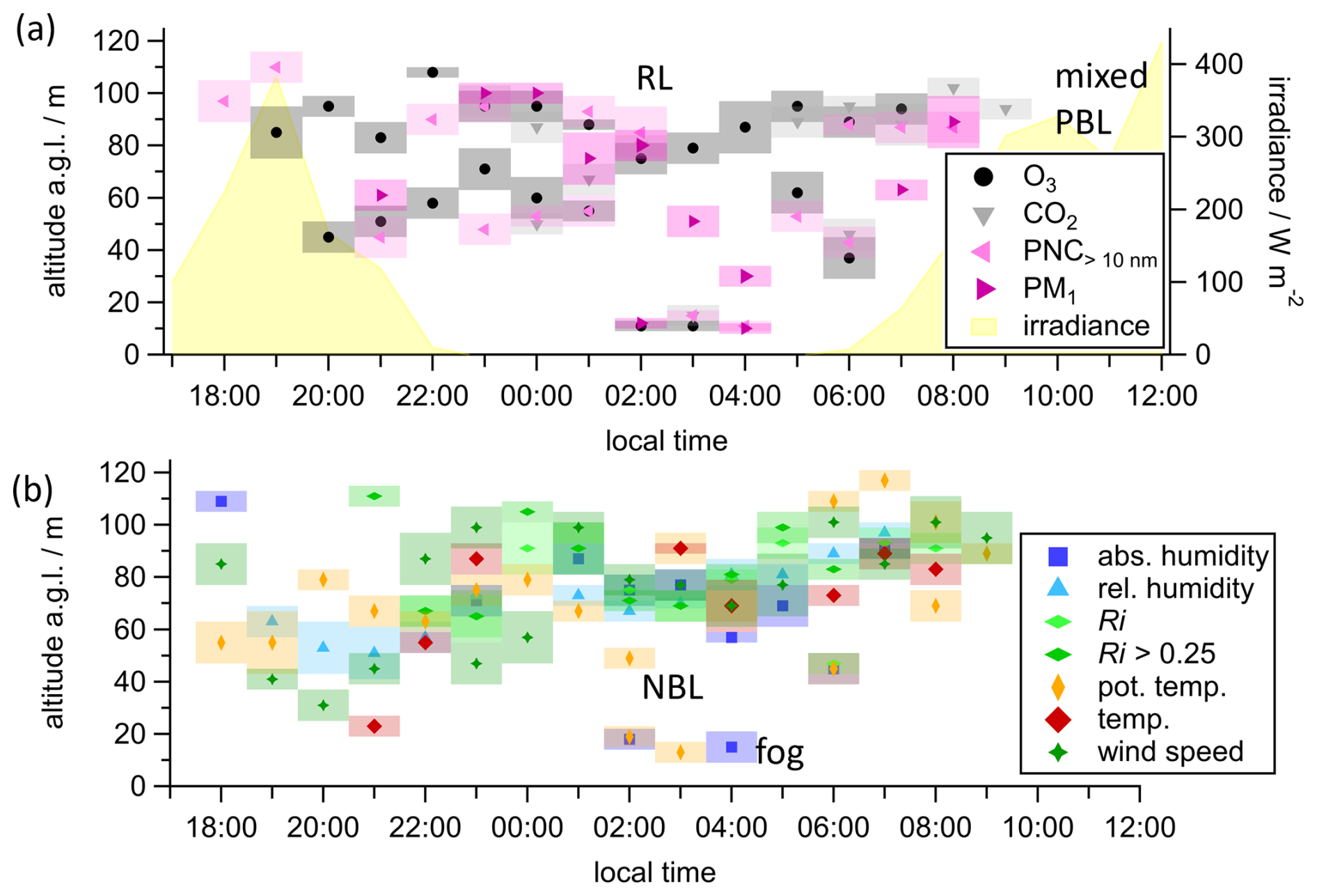
Figure 1 Estimated boundary layer heights (solid markers, with uncertainty ranges depicted as shaded areas) during the night of 20 to 21 June 2024. The boundary layer heights were derived from strongest gradient changes of the respective trace matter variables (a) and meteorological variables (b) and when the criterion Ri > 0.25 was fulfilled. The yellow shaded area in (a) represents the measured irradiance, which was reduced by cloudiness in the afternoon and the late morning.

Figure 1 depicts all determined 1 h-MLHs and shows that a nocturnal cycle is discernible in MLHs determined, both from trace matter and from atmospheric variables. Even before sunset at 22:00, vertical profiles of all variables suggest layers in different heights across the 120 m altitude range. After sunset until 02:00, a layer top was observed at (50 ± 30) m with a strong spread between variables, which slightly ascended to (75 ± 10) m while the spread narrowed. Changes in gradients of trace matter and thermodynamical variables indicates a thermal and material mixing layer height in the same range. Cooling of the ground due to weakening irradiance likely forms this inversion layer, which hinders buoyancy-driven transport of trace matter above the inversion layer height. This process explains the tightness of the thermal and material mixing layer height and defines the upper boundary of the NBL. After 05:00 in the morning, this uppermost (within the probed altitude range) detected ML boundary was slightly lifted from (75 ± 10) m to (100 ± 20) m and then disappeared after 10:00 in good agreement especially with MLHs determined from dynamical and thermal variables. A material MLH is less pronounced after 08:00, likely due to enhanced mixing at this layers' intersection, which weakens material gradients. Based on this general analysis, the lower layer is attributed to the NBL and the upper layer to the residual layer (RL) as they are the most prominent nocturnal layers.

In addition to the determination of the NBL height, the highly time-resolved profiles of various variables allowed the identification of atmospheric processes behind three fine-structured layers that temporally formed in the lowermost 120 m: a descending layer between 23:00 and 01:00 from above 120 m down to 100 m, a shallow layer between 02:00 and 04:00 below 10 m and an additional layer in the NBL reaching from the ground up to 50 m from 05:00 to 08:00, while the NBL height was ∼ 90 m.

The descending ML top (from 23:00 to 01:00) relates to a material and dynamic MLH, which is primarily detected by abrupt changes of the trace matter gradients (O₃, CO₂, and PM₁) and of wind-related variables (Ri and wind speed), respectively. The first layer situated above the NBL is likely part of the RL that remained from the previous day. We also observe a second ML being part of the RL subsidizes down to the upper boundary of the NBL. The enhanced dynamical stability in this upper ML can result from a decoupling of the RL from the surface, while keeping a high stability despite faster winds in this altitude range. The descent of this layer suggests a sinking inversion, and is indicated by suddenly enhanced vertical trace matter gradients. The gradients suggests that the upper air mass originate from more distant regions or was less affected by local and surface-bound emissions, underlining that the uppermost depicted layer can be related to a completely different air mass and explains the coupling of the material to dynamical MLH. Starting at 01:00, the separation between the RL and this distantly-influenced ML vanishes, which indicates a weakening of the inversion layer after at least 3 h after its first observation.

Furthermore, independent of the establishment of a well-developed NBL, the absolute humidity- and potential temperature (θ)-profiles indicate the formation of a colder humid shallow layer up to 10 m above ground at 02:00, 1 h before the ground-based measurement station recorded a fog event. While the fog thickened, in Fig. S4 the ground-based station detected a swelling of particles, indicated by an increase of PM₁, and reduced O₃ possibly through reaction with soil-emitted NO triggered by highly humid conditions (Andersen et al., 2024). MLHs with a boundary in 10–12 m above ground were derived from vertical gradients of PNC and O₃ and agree with those from absolute humidity- and θ-profiles. In contrast to the previous subsidising fine-structure, local thermodynamical processes lead to the formation of a thermal mixing layer that 1 h later, results in the formation of a martial mixing layer.

A third fine-structure in the stratification was identified at 05:00 in (50 ± 10) m and lasted for 4 h until its dissipation before 09:00. Apparently, the preceding fog event initiated the formation of a cold pool during night (Chachere and Pu, 2016), which converts turbulent energy into an upwards directed latent heat flux and may have formed a shallow inversion layer in (45 ± 5) m above ground (Wilson and Fovell, 2016). Fig. S5 shows that despite irradiance levels during this morning are similar to the campaign's morning mean, turbulent kinetic energy is a magnitude lower than usual at this time of the day, while latent heat flux remains unaffected and still increases until the air is dried to 75 % RH. After the fogs' disappearance at 06:00, the chemical influence of the fog on trace matter markers (CO₂, O₃ and PM₁) is diminished. However, their vertical gradients seem to be more sensitive for the identification of this layer than meteorological variables (except for 07:00 in 45 m). It was not possible to detect the layer using thermodynamic stability indicators like θ or Ri, likely due to relatively small variability of the already low amount of energy at night, while the distribution of CO₂, O₃ and PM₁ near ground is limited by the available turbulent energy for mixing. As, after sunrise, radiative heating starts warming the ground, this lowermost layer dissipates 2 h prior to the NBL, which emphasises the sensitivity of this stratification. This third example of the fine-structure analysis shows that the spatially highly-resolved vertical profiles are not only capable of identifying mesoscale phenomena such as sinking inversions, but also of revealing favourable local conditions for fog and of characterizing the vertical extent of fog events. As shown in this example, using trace matter variables to estimate a material MLH can be helpful to differentiate layers under dynamically weak conditions, where meteorological indicators might fail.

These analyses of the NBL fine-structure using hourly vertical profiles of multiple variables show that there is a strong difference between the power and potential of different variables to detect details in atmospheric stratification. We could show that in the early night, a dynamical MLH goes along with a material MLH, due to long-range transport. In contrast a developing fog event was identified using a thermal MLH even before it was observable using a material MLH, while a dynamical MLH was absent in a similar altitude range. A material MLH still indicated the slow recovering of the fog's aftermaths. The absence of a dynamical and thermal MLH at this time in this altitude range highlights the low dynamics due to a lack of energy, which could be converted by latent heat that hinders convective mixing.

In respect to individual variables, the profiles of O₃ and θ provide MLH information in 22 and 19 times, respectively, with multiple MLs being detected in a single vertical profile throughout the night from 18:00 to 10:00. In contrast, the air temperature and the Ri= 0.25-criteria indicated a MLH in only 8 profiles each. Under low winds (here 0–2 m s⁻¹ near ground), Ri does not work as a reasonable indicator and dynamic MLH are hard to identify. O₃- and θ-profiles even provide information on multiple layers in 7 profiles during the night, whereas the other variables typically reveal information on double layers only once or not at all. O₃ and θ appear therefore to be the most sensitive indicators for thermal and material MLHs, and fine scale stratification detection. Hence, they are recommended for nocturnal MLH detection. Nevertheless, as a best-practice, we suggest to confirm MLHs determined by any indicator using multiple other variables, also to understand its formation background and the underlying dynamics that often cannot be interpreted from a sole variable alone.

This analysis demonstrates that:

• a.

  Highly spatially- and time-resolved vertical profiles of various variables are essential for detecting shallow layers.

• b.

  While meteorological variables are necessary for characterizing the dynamical and thermal properties of air masses, trace matter variables offer a different perspective on material accumulation and stratification due to various atmospheric processes, especially in the NBL. A combined approach enhances the sensitivity and accuracy of MLH detection.

• c.

  Trace matter variables can provide information about stratification even when dynamic influences are minimal.

However, there remains a need for objective stratification detection algorithms, as manual estimations of MLHs can be subjective and may lead to misinterpretation.

4 Influence of solar irradiance on trace matter distribution

After sunrise, radiative heating of the ground increases instability of the NBL leading to enhanced sensible heat flux and vertical convective mixing through the formerly stable NBL. The PBL becomes more convective and grows vertically, mixing in more and more air from the RL. Although this relationship is widely recognized, the impact of solar irradiance on the distribution of trace matter in the lowermost troposphere remains an active area of research (Rowlinson et al., 2025; Deot et al., 2025).

Site selection for ground-based measurements typically focuses on horizontal representativity, whereas vertical representativity within the mixing layer – where stations are often located – is commonly assumed to be “sufficient”. This assumption is typically idealized. In practice, the PBL is frequently treated as a single, well-mixed layer with only its height being diagnosed, neglecting vertical gradients, fine-scale stratification, dynamical processes and temporal variability of MLHs. Here, we investigate the influence of solar irradiance on the vertical distribution of trace matter, their gradients, and to which extent ground-based measurements describe the conditions in the PBL accurately, particularly under convective conditions. Recent studies differentiate between a dynamical, thermal, and material PBLH that can originate from different atmospheric processes as already shown in Sect. 3 (Tan et al., 2025). In summer time, especially during daytime, these PBLHs are tightly coupled, hence a further differentiation is not required here (Xin et al., 2026).

4.1 Classification of “clear-sky” and “cloudy” days

All measurement days during BISTUM23 and BISTUM24 could be categorized as “B/C” (moderately/slightly unstable) according to the Pasquill-Gifford stability categories (Gifford, 1961). This scheme is traditionally used to classify the atmosphere regarding its stability, based on wind speed and solar irradiation. Since wind speeds depend strongly on local topography and Pasquill-Gifford methods often fail to identify daytime instability at many sites (Kahl and Chapman, 2018), especially in the “B/C” regime, further classification is necessary.

For simplicity, we categorize measurement days throughout the campaigns into “clear-sky” and “cloudy” depending on the integrated daily solar irradiance that reached the measurement site. A strong correlation (Pearson's r²= 0.74, Fig. S6) between sensible heat flux measured in 5 m above ground and irradiance during BISTUM24 (30 min-averages) suggests that irradiance can be used as a proxy for solar radiation-driven mixing, especially in the lower part of the PBL (Behrendt et al., 2020). Noting, that, there are additional drivers for sensible heat flux apart from irradiance which we do not regard in this study (Lu et al., 2024). The classification was performed on a daily basis for simplicity and more importantly due to the fact that any shorter time spans would still be influenced by effects from previous conditions lasting for several hours, such as evaporation from ground or a PBLH that results from the cumulative irradiance. After each day, the PBL is reset naturally and needs to be re-formed from irradiance-driven turbulence making this a comparable time span. For BISTUM23 and BISTUM24, the unimpeded average hourly solar irradiance was calculated from local photometer measurements under perfectly cloudless conditions. Based on these data, we categorize measurement days throughout the campaigns into “clear-sky” (> 75 % of the potential maximum of daily integrated irradiance) and “cloudy” (up to 75 %). Days with rainfall (> 0.5 mm h⁻¹) were also classified as “cloudy”, independent of their daily integrated irradiance, to account for evaporation-driven gradients (Fig. S7), resulting in a total number of 4 “clear-sky” and 10 “cloudy” days for BISTUM23 and 5 “clear-sky” and 10 “cloudy” days for BISTUM24. Results from a sensitivity study in Sect. 4.2 considering respective irradiance thresholds of 65 %, 75 %, and 85 % demonstrate that the 75 % criterion is reasonable to observe clear differences, between “clear-sky” and “cloudy” days.

Average hourly UAS-based 500 m-vertical profiles were calculated for all measured variables from both campaigns for the time intervals from 08:00 until 21:00. Hours of the day represented by only a single available profile within a campaign and cloudiness-class were excluded from further analysis. The procedure resulted in 42 hourly vertical 500 m-profiles under “clear-sky”-conditions during BISTUM23 and 70 profiles during BISTUM24. In comparison, 42 and 59 vertical 500 m-profiles were probed during “cloudy” days during BISTUM23 and BISTUM24, respectively. The number of profiles with respect to the number of measurement days is relatively smaller for both campaigns for the “cloudy” days due to the often less favorable flight conditions on these days, compared to “clear-sky” days. On average, the daily mean irradiance during “cloudy” days was 170 W m⁻² (−36.6 %) smaller than for “clear sky” days for BISTUM23 and 178 W m⁻² (−33.5 %) smaller for BISTUM24 (calculated for 13 h of irradiance > 50 W m⁻²); the daily mean precipitation during “cloudy” days was 3.0 mm (BISTUM23) and 3.5 mm (BISTUM24). larger than during “clear sky” days These results suggest comparability of both campaigns, although measurement site-specific influences (sources, sinks, heat reservoir, etc.) and different weather events, especially on “cloudy” days, can significantly affect the lower tropospheric structure due to cold pool formation, additional stratification and air mass entrainment (Moormann et al., 2026). In contrast, “clear-sky” days are expected to be more similar due to the dominance of irradiance-driven convective mixing.

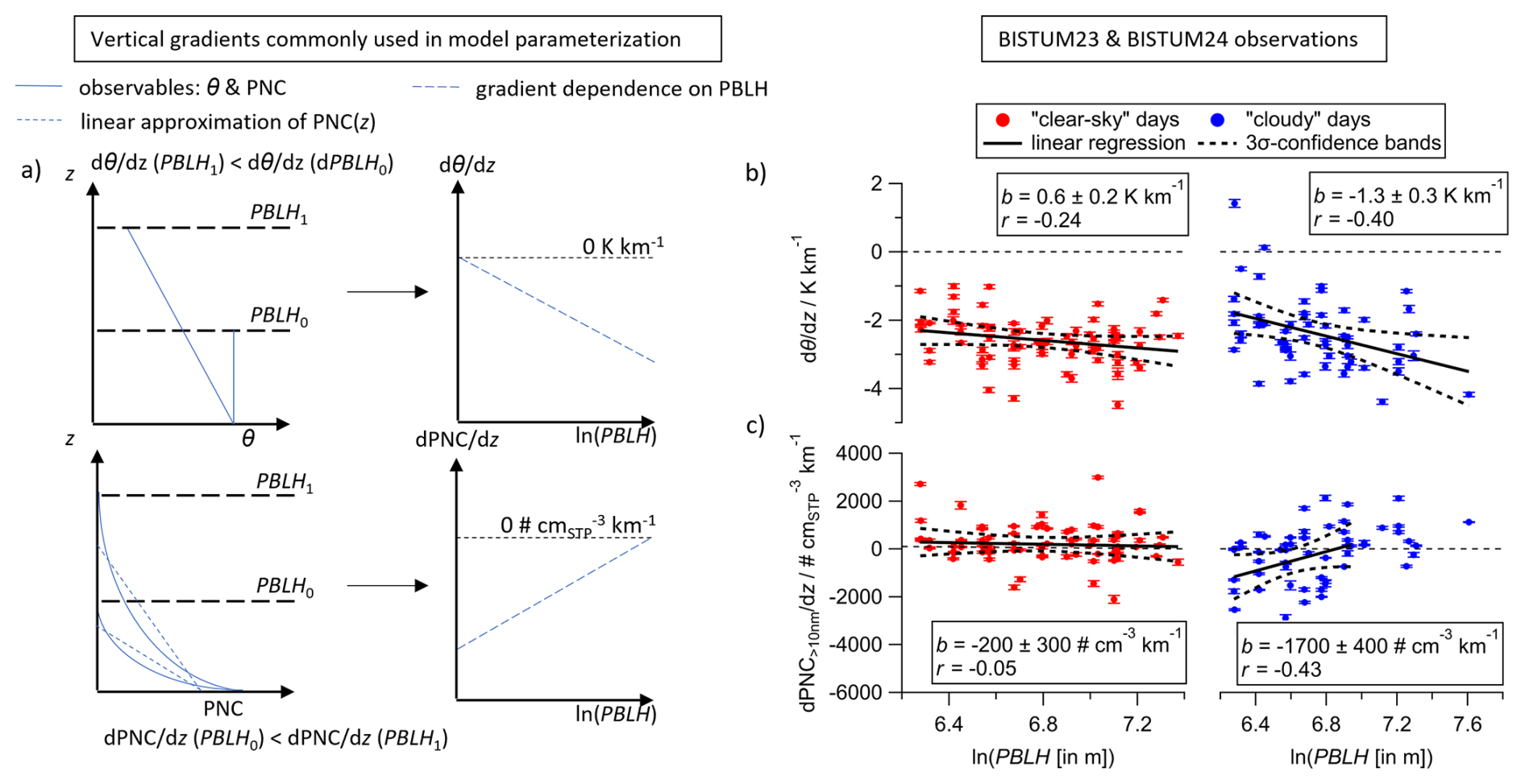
Figure 2 (a) Schematic description of the dependency of atmospheric stability (reflected by θ(z), with the altitude z) and a pollutant with source at ground level (PNC(z)) on altitude for the well-mixed planetary boundary layer with a height PBLH_i as commonly used in model parameterizations (a, left). Deriving the dependence of d$\mathit{\theta }/\mathrm{d}z$ and $\mathrm{d}PNC/\mathrm{d}z$ from PBLH results in a linear-logarithmic dependency of respective gradients on the boundary layer height (a, right). Experimental data of gradients of the potential temperature θ (b) and the particle number concentration PNC_> 10 nm (c) in the lowermost 500 m in a mixed PBL from both campaigns are plotted versus associated logarithms of respective planetary boundary layer heights (PBLH, in m). Linear regression with the slope b and its 3σ-confidence bands are depicted in solid and dotted lines.

4.2 Influence of solar irradiance on trace matter gradients in the PBL

The direct influences of solar irradiance on the mixing and vertical distribution of trace matter variables in the PBL are not considered in Lagrandian modelling tools that are commonly used to study vertical pollutant transport: FLEXPART represents turbulent vertical dispersion but shows low agreement with observations near the surface under slightly unstable conditions (Hanna, 1984; Bakels et al., 2024). LAGRANTO computes air-parcel trajectories and can be used to identify air flow pathways and synoptic scale structures, but lacks turbulence, microphysical changes of air parcels and their surface interactions (Sprenger and Wernli, 2015). These convective transport schemes equate strong irradiance with an increased PBLH, based on two assumptions:

• a.

  The PBLH scales with the solar radiation, which enhances the atmospheric instability, i.e., stronger irradiance enhances the instability that drives the PBLH upwards.

• b.

  The PBLH solely depends on the driving instability and turbulence in the PBL and further lifting is not affected by aloft layers, e.g., inversion layers that hinder further PBLH increase.

In general, a high PBLH is associated with stronger turbulent vertical mixing by larger eddies and consequentially with weaker trace matter gradients. Hence, both assumptions allow estimation of the vertical distribution of trace matter for situations when the PBLH increase is unhindered, but could be misleading, when radiative convection does not scale with the PBLH. More stable air masses aloft that result from the synoptic meteorological conditions and cannot be ruled out and thus, always should be considered. The correlation of the PBLH with irradiance on “clear-sky” (r²= 0.86) is enhanced compared to that on “cloudy” days (r²=0.57), especially during BISTUM23. Differences in the slopes scaling of the PBLH with irradiance between BISTUM23 (1.38 W m⁻¹) and BISTUM24 (1.97 W m⁻¹) highlight difficulties when applying these assumptions universally on different measurement sites (Fig. S8).

4.2.1 Driving force of convective mixing: Irradiance vs. PBLH

To investigate the influence of irradiance on the vertical gradients of trace matter, we examine the dependence of gradients d$\mathit{\theta }/\mathrm{d}z$ and dPNC${}_{>\mathrm{10}\mathrm{nm}}/\mathrm{d}z$ on the PBLH. The gradients were estimated from in-situ data of the lowermost 500 m. The PBLH was derived from the ICON-D2 model as described in Sect. 2.2. We differentiated between “clear-sky” and “cloudy” days to account for different radiation intensities and only considered data when a single layer was probed, i.e., PBLH > 500 m and a mixed layer can be assumed throughout this altitude range, which was typically after 12:00. Within a well-mixed PBL, several meteorological variables such as the temperature, absolute humidity, or wind speed show a linear dependency on the logarithm of the altitude (Stull, 1988). A similar trend is expected for concentrations of trace matter that are emitted at ground and dilute with altitude. Figure 2a shows that with lower PBLH (z₀) this vertical profile is compressed, intensifying the gradients of the variables, whereas a deep PBL (z₁) stretches the profile, attenuating the gradients.

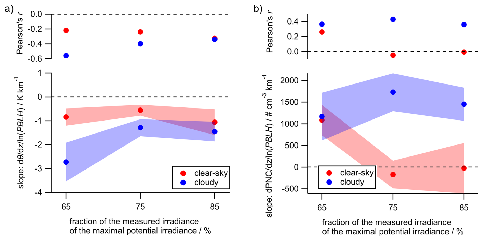
Figure 3 Influence of the irradiance threshold as a criterion to separate “clear-sky” (red) and “cloudy” days (blue) on the dependency of d$\mathit{\theta }/\mathrm{d}z$ and dPNC${}_{>\mathrm{10}\mathrm{nm}}/\mathrm{d}z$ on the PBLH (in m). Pearson's correlation coefficient r and slopes of the respective gradients versus the logarithm of the PBLH are depicted with 1σ-confidence bands. The classification criteria are the ratios of the measured irradiance in respect to the maximal potential irradiance.

Firstly, we analyze the gradient of the potential temperature d$\mathit{\theta }/\mathrm{d}z$ as a surrogate for static stability and turbulent mixing, where more negative d$\mathit{\theta }/\mathrm{d}z$ indicates greater instability and larger positive values indicate increased stability. We test our in-situ data for a linear relationship between d$\mathit{\theta }/\mathrm{d}z$ and the natural logarithm of the PBLH (ln(PBLH)) above ground level to assess the applicability of the parameterization scheme for atmospheric instability, used in previously named vertical transport models (Fig. 2a), to our ambient data (Fig. 2b) before using the same method on vertical gradients of aerosol particle concentrations (Fig. 2c). In Fig. 2b, hourly d$\mathit{\theta }/\mathrm{d}z$-data from both campaigns were combined assuming that differences in the gradients originate primarily from different PBLHs rather than from measurement site's influences, noting that also the local topography can influence the PBLH.

On all investigated “clear-sky” and virtually all “cloudy” days, d$\mathit{\theta }/\mathrm{d}z$ is negative, and the correlation plot shows a further decrease with increasing PBLH (Fig. 2b) indicating enhanced atmospheric instability increases the PBLH. This is consistent with enhanced convective turbulence in deeper PBLs. Despite similar trends for both cases, this dependency of d$\mathit{\theta }/\mathrm{d}z$ on the ln(PBLH [in m]) is more pronounced on “cloudy” days (slopes for “clear-sky” days: (−0.6 ± 0.2) K km⁻¹, Pearson's r= −0.24 and “cloudy” days: (−1.3 ± 0.3) K km⁻¹, r= −0.40). Under “clear-sky” days the weaker relationship of d$\mathit{\theta }/\mathrm{d}z$ with ln(PBLH), shows that further PBLH lifting is mainly hindered by stable air masses aloft than by missing internal radiative convection.

Figure 2c shows the relationship between vertical gradients of the PNC_> 10 nm (dPNC${}_{>\mathrm{10}\mathrm{nm}}/\mathrm{d}z$), which is a reliable pollutant tracer with a low measurement uncertainty, and ln(PBLH). In a perfectly mixed layer that is capped by a strong inversion layer, neither a vertical gradient nor an influence of the PBLH on the vertical gradient of PNC_> 10 nm is expected. This is observed on “clear-sky” days (red in Fig. 2c, r= −0.05), suggesting efficient mixing of the PBL during all flights. Contrary, on “cloudy” days, dPNC${}_{>\mathrm{10}\mathrm{nm}}/\mathrm{d}z$ is negative for small PBLHs, suggesting a source of particles near ground and imperfect mixing. For larger PBLHs, associated with stronger turbulent mixing, the gradient of particle concentrations increases (r=0.43) and vanishes for PBLHs above ∼ 1300 m (ln(PBLH [in m]) = 7.2); a positive dPNC${}_{>\mathrm{10}\mathrm{nm}}/\mathrm{d}z$ can only be explained by sinks at the ground or advected inhomogeneous air above the ground. Similar dependency and correlations were found for the non-logarithmic PBLH (Fig. S9). This observation shows that on “cloudy” days, the PBLH is a useful indicator for the mixing conditions, whereas on “clear-sky” days irradiance-driven turbulence appears sufficient to homogenize PNC_> 10 nm largely independently of PBLH.

The irradiation threshold (75 % of potential maximum of integrated daily irradiation) to separate “cloudy” and “clear-sky” days was arbitrarily selected. Therefore, a sensitivity study was performed to evaluate the reasonability of this irradiance threshold using the same gradient-based analysis approach for different threshold values. In this exercise, days were classified as “clear-sky”, when respectively > 65 % or > 85 % of the maximal potential irradiance was measured at the measurement site.

Figure 3 shows differences in the dependencies of d$\mathit{\theta }/\mathrm{d}z$ and dPNC${}_{>\mathrm{10}\mathrm{nm}}/\mathrm{d}z$ on the PBLH for “clear-sky” and “cloudy” days for the various threshold criteria. In Fig. 3a d$\mathit{\theta }/\mathrm{d}z$ does not show a dependency on the PBLH for “clear-sky” days for any threshold value. In contrast on “cloudy” days, d$\mathit{\theta }/\mathrm{d}z$ depends stronger on the PBLHs for the 65 % threshold criteria compared to less negative d$\mathit{\theta }/\mathrm{d}z$-ln(PBLH) relationships for 75 % and 85 %. The negative d$\mathit{\theta }/\mathrm{d}z$/ln(PBLH) agrees with the textbook example from Fig. 2a. The atmospheric stability is less stable for lower PBLHs under the 65 % threshold criteria, due to, e.g., frontal situations that are often associated with cloudiness. Days with frontal situations, i.e., enhanced atmospheric instability, contribute stronger to days under the 65 % threshold than to 75 % or 85 %, leading to a relatively high correlation of d$\mathit{\theta }/\mathrm{d}z$ and ln(PBLH) of r=0.57. For the relationship of $\mathrm{dPNC}/\mathrm{d}z$ from ln(PBLH) no difference between values for “clear-sky” and “cloudy” days is observed for the 65 % irradiance threshold, while for thresholds of 75 % and above, a clear difference between both irradiation classes is found. This observation suggests that an irradiance threshold of 75 % is necessary and sufficient to separate the effects of irradiance-driven mixing and of PBLH on the vertical gradients of particle concentrations We conclude that using “75 % of the maximal potential irradiance” is a reasonable threshold criterion for the simple classification between “clear-sky” and “cloudy” days, which allows usage of the irradiance to describe properties of the trace matter distribution.

Summarizing, irradiance plays a crucial role in controlling mixing in this grassy, hilly terrain. To finally understand irradiance-driven convective transport processes, similar studies spanning a broader range of irradiance levels and PBL depths in regions with different heat reservoirs and turbulence regimes that can influence convective mixing (e.g., rainforests, polar areas) would be valuable.

4.2.2 Diurnal variation of trace matter gradients

The previous section indicates that besides irradiance and the PBLH, sources and sinks in any part of the vertical range of the PBL can shape the gradients of aerosols in the boundary layer. These sources and sinks are not necessarily permanent and can vary with daytime. To enhance the understanding of such processes, we computed hourly vertical gradients for both campaigns within the 0–500 m column; non-zero gradients indicate an inhomogeneous distribution of a variable, that can be due to its natural dilution from local sources and sinks which can lead to stratification (i.e., an incompletely mixed layer). Absolute magnitudes of the gradients could be used for comparison to other measurement sites. However, absolute gradients reaching up to a few hundreds of meters into the PBL are sparse in literature. Such a literature comparison is beyond the scope of this manuscript.

We discuss the diurnal variation of gradients of CO₂, O₃, and PNC_> 10 nm (Fig. 4), which are often measured ground-based in atmospheric studies. These variables cover a range of different behaviors, as CO₂ is a chemically inert anthropogenic tracer, frequently originating from ground-level sources like industrial production or vehicle exhaust with a daytime vegetation sink, also at ground level, whereas O₃ is more reactive and is depleted via reactions with NO and unsaturated volatile organic compounds as well as by photolysis (Atkinson et al., 1992; Olszyna et al., 1994). For a general understanding, a rough comparison of the efficiency of physical and chemical loss mechanisms might be useful to demonstrate the relevance of different loss pathways. The chemical loss of O₃ by reaction with NO can be estimated by using the rate constant $k_{\mathrm{NO}+{\mathrm{O}}_{\mathrm{3}}}=$ 1.9 × 10¹⁴ cm³ molec.⁻¹ s⁻¹ and a reasonable NO concentration [NO] ≈ 0.1 ppbv during night and [NO] ≈ 0.5–1.0 ppbv during daytime (Dewald et al., 2022; IUPAC, 2025), resulting in lifetimes ${\mathit{\tau }}_{\mathrm{chem}}=\frac{\mathrm{1}}{k_{\mathrm{NO}+{\mathrm{O}}_{\mathrm{3}}}\left[\mathrm{NO}\right]}\approx$ 30–60 min during daytime and up to 10 h in the night. Physical loss due to diffusion can be estimated by the related lifetime ${\mathit{\tau }}_{\mathrm{diff}}=\frac{L^{\mathrm{2}}}{K_z}$ with the vertical length L and the eddy diffusivity K_z. Assuming L= 25 m for the vertical range that is relevant for chemical processes, and K_z ≤ 0.1 m² s⁻¹ for moderately stable conditions as in the morning and during night time (diffusion dominated) and K_z ≈ 1 m² s⁻¹ for convective conditions as during the day (turbulence dominated) above grassland (Stull, 1988). We can now estimate a diffusion-related lifetime τ_diff= 2 h for stable and a convective-related lifetime τ_conv= 10 min for convective conditions. The lifetimes τ_chem and τ_diff are in a similar range, while convective conditions reduce the lifetime. This shows that chemical and physical loss are both relevant depletion pathways and mainly depend on the convective conditions and prevalent NO levels.

PNC_> 10 nm reflects processes in the particle phase and can be influenced by anthropogenic emission sources at ground level or by new particle formation (NPF). Figure S2 shows that, although polluted air doubles the particle number concentration, anthropogenic air masses advected from the Frankfurt area are already well-mixed at the measurement site and do not show a gradient in PNC_> 10 nm. Continuous size-resolved particle size distribution measurements (> 7 nm) by MoLa at ground level indicate NPF starting around noon on most days, when NPF-precursors are well-mixed in the lowermost layers (Fig. S10). Therefore, NPFs happens along the whole vertical range. Conclusively, the gradient of particles, observed in the morning, is likely due to regional emissions near the ground, when convection has not homogenized the material PBL, yet.

In the morning and the evening hours, all three variables CO₂, O₃, and PNC_> 10 nm show substantial gradients across the 500 m-column. The periods between 12:00 and 20:00 (highlighted in yellow in Fig. 4) allow the investigation of gradients within a single mixing layer as the MLH is larger than 500 m; as a consequence the vertical profiling with FLab results in insignificant gradients in the lowermost 500 m for CO₂ and O₃, despite O₃ mixing ratios generally increase in the troposphere with altitude (Roelofs and Lelieveld, 1997) and CO₂ is generally emitted at or near ground level. Slightly negative gradients of CO₂ are probably observed due to emission near ground and dilution with altitude. Similar observations on “clear-sky” and “cloudy” days reveal little influence of the irradiance on the distribution of both trace gases. For the same period, an insignificant gradient for PNC_> 10 nm is observed on “clear-sky” days for BISTUM23 and BISTUM24 (see Sect. 4.2.1), indicating nearly complete irradiance-driven mixing. On “cloudy” days when convective turbulence is expected to be lower, negative gradients of PNC_> 10 nm are apparent, reflecting reduced vertical transport for BISTUM23 and until 15:00 for BISTUM24.

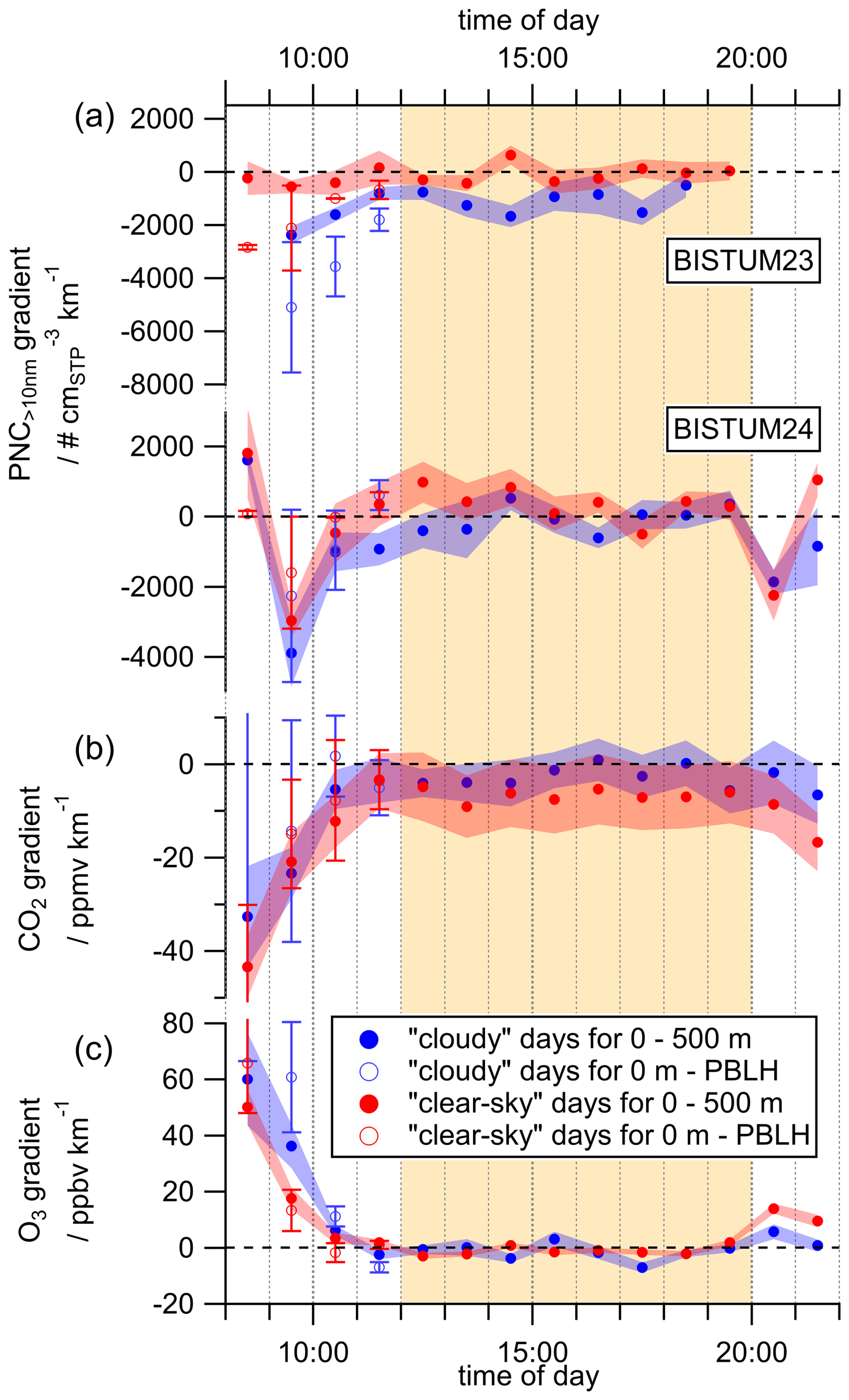
Figure 4 Average hourly-resolved gradients of PNC_> 10 nm (a), CO₂ (b) and O₃ (c) in the lowermost 500 m above ground show a diurnal variation for “clear-sky” (red) and “cloudy” days (blue). Open markers represent gradients and ratios calculated for measurements solely within the PBLH, when PBLH was lower than 500 m. The yellow shading represents hours with the PBLH being higher than 500 m. Propagated uncertainty bars (1σ) are presented as shaded areas.

Before 12:00 and after 20:00, the gradient within the lowermost 500 m has been determined across multiple layers, e.g., the NBL and the RL (see Sect. 3). In addition, gradients have also been calculated only for the lowermost layer (empty circles in Fig. 4), i.e., within an increasing altitude range from 08:00 to 12:00 that only covers the forming lowermost mixing layer. The NBL height, which limits the respective altitude range, was estimated from sudden changes in the gradients of the mean vertical profiles of CO₂, O₃, PNC_> 10 nm, and θ at the particular hour for all measurement days. Although, the lowermost layer is assumed to be well-mixed, the gradients are not consistently lower compared to when probing across multiple layers at the same time. This may be due to high day-to-day variability of the PBLH in the morning hours as its dissipation depends on the available convective strength, the stability of the RL aloft, and that vertical mixing has not equilibrated the vertical distribution already. Figure 4 shows that the difference of gradients up to the NBL height and 500 m-range gradients systematically align with increase of the MLH, i.e., with daytime until noon. For lower PBLHs, sinks and sources of the aerosol at the surface are more strongly weighted in gradients as the fractional contribution of the lowermost bin increases with a lower number of considered altitude levels, causing non-zero gradients as well.

In conclusion, sources and sinks near/at the ground play an important role on gradients, especially when convective mixing is not strong like in the morning. Despite the variety of influences on the trace matter distribution, the gradient comparison of CO₂, O₃, and PNC_> 10 nm between “clear-sky” and “cloudy” days before 12:00 indicates that enhanced irradiance contributes to lower gradients and a more homogeneous distribution, as expected.

4.3 How representative are ground-based measurements?

The analysis of nocturnal MLHs (Sect. 3) and the diurnal variability of trace matter distribution in the lowermost 500 m (Sect. 4.2.2) highlight that stratification significantly affects vertical gradients of meteorological and trace matter variables. In Sect. 4.2.1, the analysis of gradients within the lowermost mixing layer further shows that atmospheric instability and vertical mixing are mainly driven by solar irradiance and that deducing turbulent mixing solely from the PBLH and surface roughness might result in significant biases (especially for strong radiative conditions). In this section, we investigate how well ground-based measurement are capable to quantitatively represent conditions in the lowermost 500 m which is sufficient to represent conditions in the ML. We used only the daily periods from 12:00 to 20:00, i.e., times without a NBL to ensure that the probed vertical 500 m-column only includes a single atmospheric layer and does not extend into another air mass aloft (Sect. 4.2.2). A metric R was developed to quantify the representativity of ground-based measurements for the lowermost 500 m and discuss the diurnal trace matter variation of the representativity (Fig. 5). We summarize the results of the representativity of meteorological and trace matter tracers within a single mixed layer in Fig. 6.

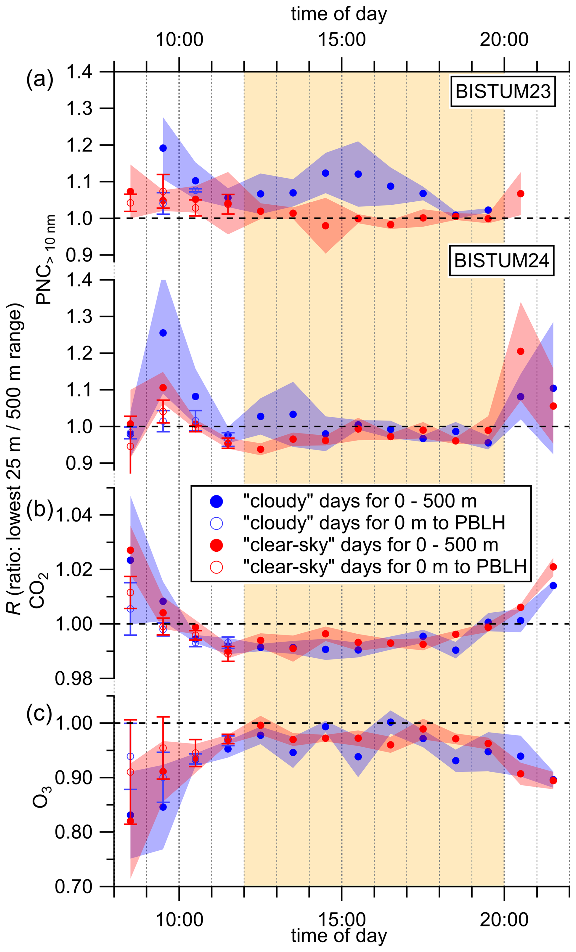
Figure 5 A diurnal variation the representativity R of PNC_> 10 nm (a), CO₂ (b) and O₃ (c) of ground-based measurements for the 500 m-column above. Open markers represent ratios calculated for measurements solely within the PBLH, when PBLH was lower than 500 m. The yellow shading represents hours with the PBLH being higher than 500 m. Propagated uncertainty for data points derived from the whole 500 m and from ground to the PBLH are represented as shaded areas and error bars as 1σ-uncertainties, respectively.

4.3.1 Metrics for representativity of ground-based measurements

In order to evaluate how well ground-based measurements can quantify and represent conditions in the lowermost 500 m of the mixing layer, we define R as a quantitative measure of the vertical representativity of ground-based measurements. R is the ratio of the mean vertical column value of the lowermost altitude bin (0–25 m above ground, for 25 m vertical resolution, from drone measurements only) for a certain variable to the respective mean column value over the lowermost 500 m range and was separately calculated for each hour and separated by time of the day, campaign, and cloudiness class. Perfect representativity is given for R=1, whereas our “ground-based” measurements overestimate mixing layer quantities (i.e., within the 500 m column) for R> 1 and underestimate them for R< 1.

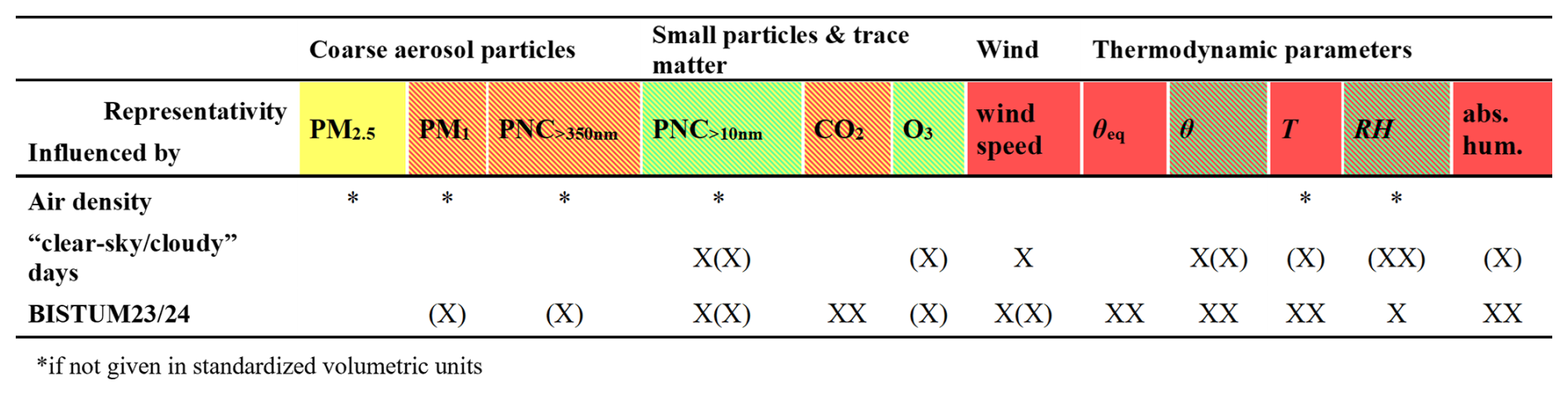
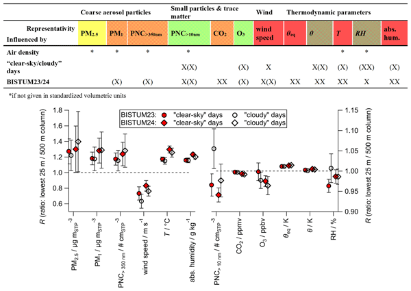
Figure 6 Representativity of ground-based measurements for various variables for the lowermost 500 m: green (very representative), yellow (mostly representative) and red (poorly representative). The pattern is striped with the respective colors, when different classification levels were identified, depending on the location or irradiance influences. The effects of decrease the of air density with increasing altitude (“^*”), and of the intensity of radiative heating and measurement location-specific influences (sinks, sources, etc.) on the representativity are additionally indicated (with “X” and “XX”, see text for definition).

The mean sampling height in the lowest altitude bin was at ∼ 9 m above ground, considering the longer hover periods in 6 m altitude in between vertical profiling flights. This mean height is suitable for comparison with typical ground-based measurements, because most ground-based stations probe air in 3–10 m altitude (Savijärvi, 2006), while sampling in 10 m is common for meteorological stations to reduce surface influences (Pastorello et al., 2020; WMO, 2025a).

An overall evaluation of how well ground-based measurements represent the conditions within the lowermost mixing layer is presented in Fig. 6. It is based on the representativity values R and their uncertainties from Fig. 7. The uncertainty bars in Fig. 7 are dominated by the variability σ of the ground-based measurements (of only a single height bin) compared to lower standard error of the mean of the 500 m column from multiple height bins. We use the uncertainty of R, σ, to assess the significance of deviations of ground-based measurements from perfect representativity for the perfectly mixed PBL (R=1). To highlight the importance of different types of influences, we consider in this assessment influences of air density, locations (BISTUM23/24), as well as irradiance (“clear-sky/cloudy” days) separately.

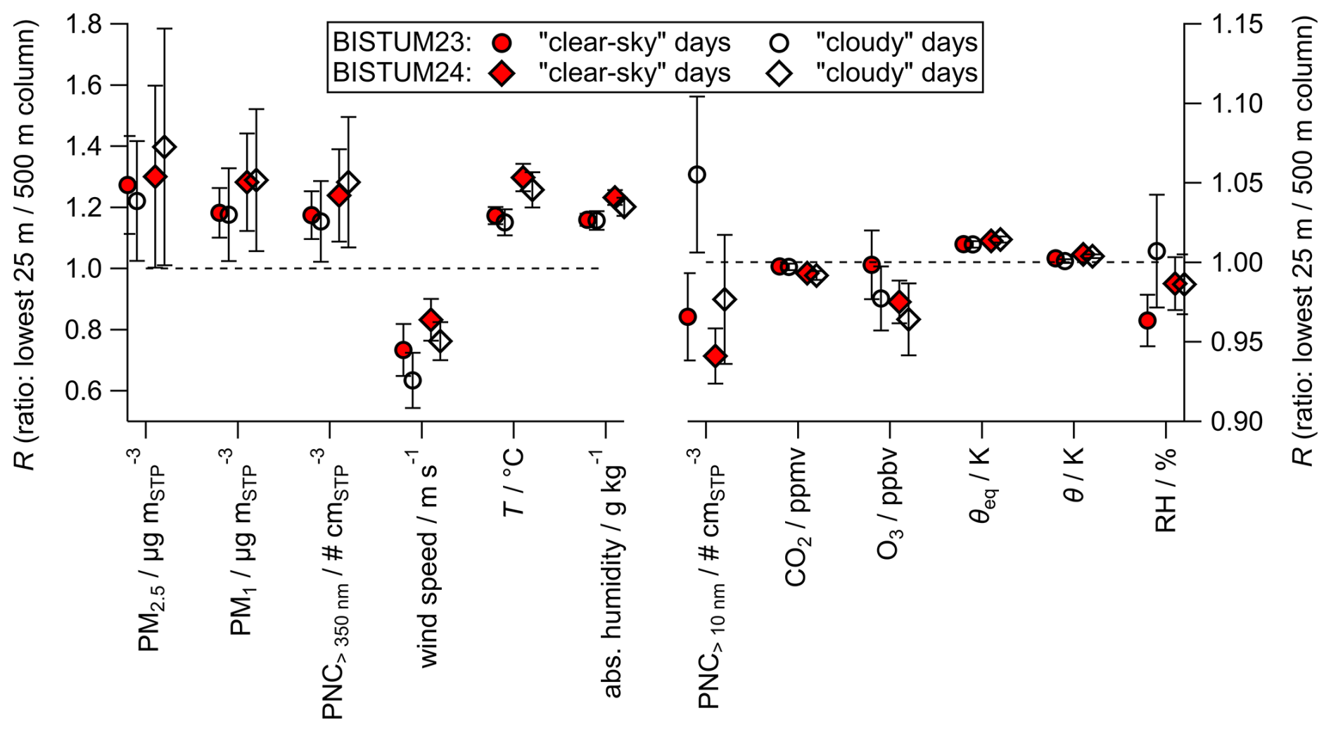
Figure 7 Representativity R (ratio of lowest 25 m/500 m column averages) of ground-based measurements with regard to the lowermost 500 m in a mixed PBL for meteorological and trace matter variables for two campaigns (circles and diamonds) for “clear-sky” and “cloudy” days (red and white filled markers, respectively). The x axis is split to enhance visibility of variables with better representativity (note the different scaling of the y axes). Error bars represent the overall uncertainty, mainly due to day-to-day variability.

The influence of air density, irradiance levels based on “clear-sky/cloudy” day, and location of the campaigns is marked in the body of Fig. 6. The “air density” changes due to reduced pressure at higher altitudes in the vertical profiles. This changes the number of particles/molecules per unit of volume as well as the temperature according to the ideal gas law. “Clear-sky/cloudy” conditions highlight different irradiance levels as already used in Sect. 4.1, while differentiation between the campaigns allow a comparison of locally specific sources and sinks at the measurement sites.

A green color in the variable name boxes in Fig. 6 depicts that very representative measurements are possible and is used if R=1 is within the ±1σ range of determined R values for the respective variable; a yellow color describes moderate representativity with the variable mean being within the ±2σ range, but outside the ±1σ range from R=1; and red highlights significant challenges for ground-based measurements with mean R values deviating > ±2σ from R=1. The pattern is striped with the respective colors, when different classification levels were identified, for different location or irradiance conditions.

For each variable, the strength of the influence of irradiance and the measurement site on R is provided: “^*” marks influence of the air density on the variables, “X” shows medium impact on R and is given, when the ratio of the propagated uncertainties (σ_A and σ_B) to the difference of R of the same influencing factor $\frac{\sqrt{{\mathit{\sigma }}_{\mathrm{A}}^{\mathrm{2}}+{\mathit{\sigma }}_{\mathrm{B}}^{\mathrm{2}}}}{\left|R_{\mathrm{A}}-R_{\mathrm{B}}\right|}$ is > 0.5 but < 1; “XX” reveals a strong impact with the ratio being > 1. “X” is written in parentheses if the respective influence occurs only for one of the irradiance or location cases, e.g., for a significant difference between “clear-sky/cloudy” days for BISTUM23, but not for BISTUM24.

The results are discussed separately for meteorological and trace matter variables in the following.

4.3.2 Diurnal variation of representative ground-based measurements of trace matter

Meteorological variables and trace matter concentrations show similar diurnal trends in representativity of ground-based measurements for the mixing layer for both campaigns. Exemplarily for BISTUM24, Fig. 5 illustrates the average diurnal variation of representativity for the trace gases CO₂ and O₃, and PNC_> 10 nm. Similar to the analysis of vertical gradients, (Sect. 4.2.2) we observe a significant over- or underestimation by ground-based measurements with respect to the 500 m-column in the morning and evening, while the deviation from perfect representativity (dotted line in Fig. 5) is minimal between 12:00 and 20:00. The main reason for this is that before 12:00 and after 20:00, multiple chemically different layers in the lowermost 500 m were considered and result in a bad representativity values. During these times, probing near the ground only, i.e., in the NBL remnant, would result in sampling lower O₃ mixing ratios, but higher levels of CO₂ and PNC_> 10 nm, compared to the RL, which consequentially results in an underestimation of O₃ and an overestimation of CO₂ and PNC_> 10 nm by ground-based measurements for the complete lowermost 500 m column. However, when only taking the lowermost layer into account (open markers in Fig. 5) the representativity by ground-based measurements for the single mixing layer improves strongly and the representativity approaches that of the measurements between 12:00 and 20:00 that are also within a single layer. In contrast to the gradient analysis, the day-to-day variability is low and less affected by the absolute trace matter levels.

Between 12:00 and 20:00, insignificant gradients of CO₂ and O₃ indicate a well-mixed layer, (Sect. 4.2.2) the measurements in the lowermost 25 m slightly underestimate the CO₂ and O₃ levels in the mixing layer by 4 ppmv and 0.4 ppbv (1 % and 3 % of the absolute levels), respectively. O₃ depletion near ground occurs frequently due to an enhanced concentration of reaction partners near ground as well as dry deposition of O₃, while O₃ mixing ratios generally increase in the troposphere with altitude (Roelofs and Lelieveld, 1997). Although CO₂ is generally emitted at or near ground level, reduced mixing ratios might be measured near ground as photosynthesis could be a significant sink in this biogenically dominated environment during the day.

O₃ and CO₂ data show similar trends in representativity between 12:00 and 20:00 on “clear-sky” and “cloudy” days. The variability of the representativity for the chemically inert CO₂ is low and similar between “clear-sky” and “cloudy” days; hence it is independent on the cloudiness/precipitation. In contrast, for R of O₃ varies by ∼ 1 % on “clear-sky” days, but it varies between 0 % to 8 % on “cloudy” days. The enhanced variability on “cloudy” days, might be due to O₃ depletion at and near the surface triggered by primary biogenic or NO emissions after rain events (which are included in the “cloudy” days), while O₃-rich air is more often entrained from the free troposphere down to 500 m on such days (Moormann et al., 2026).

While the distributions of trace gases are weakly affected by irradiance, the influence of irradiance-driven mixing is stronger for PNC_> 10 nm (see Sect. 4.2.1). Strong vertical mixing allows representative ground-based measurements for the lowermost 500 m during BISTUM23, in contrast to BISTUM24, where measurements in the lowest 25 m-increment typically slightly underestimate the PNC_> 10 nm by up to 6 % until 15:00 (Fig. 5) for “clear-sky” days. Potential reasons are particle sinks at ground level, particle entrainment/advection at higher levels, albeit we do not have an explanation for this observation.

In general, diurnal profiles of CO₂, O₃, and PNC_> 10 nm show that ground-based measurements represent the lowermost mixed atmospheric layer well, however the dynamically changing PBLH influences the altitude range for which ground-based measurements are representative. Even within a “mixed” atmospheric layer, the representativity can be decreased by sources and sinks that influence trace matter in the gas and particle phase and dominates over the balancing effects of vertical mixing. Even though CO₂ is chemically inert, the interaction at the surface (emission, photosynthesis) prevents the compound for being an optimal tracer for PBLH analysis.

4.3.3 Representativity of ground-based measurements in a mixed PBL

The overall representativity of ground-based measurements for the lowermost 500 m for trace gases and meteorological variables is summarized in Fig. 6 based on the metrics in from Sect. 4.3.1 with respect to the periods from 12:00 to 20:00 when only a single layer, i.e., the lower part of the PBL, was probed (Fig. 7). As the PBLH varies depending on its definition, for example, whether it is identified as dynamical, thermal, or material PBLH, a 10 % variability between different PBLHs in summer would result in a 10 % change in the gradients of the variables in Fig. 4. However, the interpretation would not substantially change under such conditions since the relative uncertainty is larger anyway. R values are even more robust since surface chemistry and diffusional losses occur in the lowest layer and would be negligibly affected by a slightly different PBLH.

Trace matter variables

The vertical distribution of trace matter is affected by the horizontal advection of clean or polluted air masses, local emissions, and vertical mixing, which reduces vertical inhomogeneities and distributes surface-influenced air in the mixing layer. An ideally mixed layer would have a negligible vertical gradient for trace matter mixing ratios. Different trace matter levels due to different air mass origins lead to a larger uncertainty when average gradients are calculated from absolute values (Fig. S11), while the R should not be affected. However, day-to-day variability in the vertical trace matter distribution above ground may lead to the discrepancy between very good and poorly representative ground-based measurements for the lowermost 500 m for a single variable in Fig. 6.

Mixing ratios of trace gas variables as CO₂ and O₃ in the stratification-free lowermost 500 m can be measured at ground with a slightly underestimation by 0 %–2 % and 0 %–6 %, respectively. The underestimation of both gases was especially strong for BISTUM24 and probably results from sinks at the ground, such as chemical depletion of O₃ and biosphere-driven uptake (photosynthesis) for CO₂ at the surface, which bias, i.e., lowers surface mixing ratios. The differences in representativity between the measurement sites are especially strong for CO₂, whose emission at ground, i.e., anthropogenic emissions, may largely balance the CO₂ sink during BISTUM23, causing a very good representativity of ground-based measurements. We further expect that with higher cloudiness, e.g., on “cloudy” days, reduced photochemical O₃ production and reduced turbulence limit in-situ O₃ production and vertical mixing, respectively, so entrainment from O₃-rich air from aloft (RL/free troposphere) cause enhanced O₃ levels at high altitudes, while O₃ levels near ground are lower. Although this effect may be relevant in single events, on average it is not significant for the comparison between “clear-sky” and “cloudy” days. An improved representativity for the whole mixing layer can be archived for ground-based measurements, when biases caused by sinks at ground level and entrainment from above during single events are taken into account.

While trace gases are frequently quantified using mixing ratios (which are independent of the pressure decrease of ascending air masses with altitude), ground-based aerosol measurements are commonly reported in volumetric concentrations that are not always standardized to standard temperature and pressure. Consequently, if vertical differences in air density are not accounted for, using ground-level volumetric concentrations to represent a well-mixed 500 m column, they will overestimate the column-mean aerosol load by ∼ 2.7 %. This bias is considered in Fig. 5 as a best practice example as ground-based measurement stations should report volumetric variables in standardized units, e.g., in m${}_{{\mathrm{STP}}^{-\mathrm{3}}}$ “standard cubic meter” at 1013.25 hPa and 298 K, in agreement with international standardization rules (EEA, 2023; WMO, 2025a).

Aerosol particles with diameters larger than 350 nm were measured on-board FLab with an optical particle counter, but only showed low concentrations, associated with poor counting statistics and consequently high uncertainty. The number and mass fractions of these particles (PNC_> 350 nm, PM₁, PM_2.5), which were inferred from near-ground measurements, tend to overestimate the corresponding 500 m-column averages by ∼ 25 % or ∼ 22 % for standardized units, respectively, albeit with large uncertainties (error bars corresponding to roughly 10 %–80 % overestimation in Fig. 7). This ratio appears to be site-dependent, although with no significant differences. Irradiance does not appear to affect the representativity of ground-based measurements for larger particles. In contrast, the representativity of ground-based measurements for the 500 m column and the vertical gradients of PNC_> 10 nm (dominated by ultrafine particles) is significantly influenced by irradiance and measurement site location. Good representativity for this variable is achieved on “clear-sky” days. The systematic overestimation of larger particles (PNC_> 350 nm, PM₁ and PM_2.5) compared to PNC_> 10 nm in the lowermost 25 m-increment with respect to the vertical 500 m profiles might be due to ground-level particle sources, which vary with the particle size, and entrainment of particle-poor air from above the surface layer. Particles in the size range from 10 nm to 1 µm are similarly mixed by eddies, hence no difference in mixing efficiency is expected for PM₁ and PNC_> 10 nm, resulting in respective lifetimes of days, by depositional removal, that should not influence the particle distribution in the PBL (Hinds, 1999). Dry deposition, which is based on surface roughness length, describes the transport efficiency of trace matter in eddies around surface obstacles, naturally varies with the measurement sites. Consequentially, differences in the ground-near sources of small particles and the surface roughness between the sites explain the small discrepancy between BISTUM23 and BISTUM24 data.

Meteorological variables

Vertical gradients of meteorological variables from both campaigns show significant influence in higher altitudes from air mass intrusion from aloft, e.g., with dry air that reduces the absolute humidity that is fed by water evaporated from ground. Reduced ambient pressure with increasing altitudes causes adiabatic cooling of ascending air masses, which forms the vertical gradient of temperature (T) and, together with moisture dilution, shapes the gradient of relative humidity (RH). The gradients of the potential temperature (θ) and equivalent potential temperature (θ_eq) are markers for atmospheric stability, hence θ accounts for dry-adiabatic effects and θ_eq also incorporates water-vapor variability. Therefore, θand θ_eq, are more versatile/standardized, when describing the properties of a mixing layer, in contrast to T and RH.

In Fig. 7, strong differences in the observed representativity are presented for all four variables especially between the locations, resulting in an “XX” (“X” for RH) in Fig. 6. The influence of different irradiance levels is only minor. Differences in heat reservoirs at ground due to various kind of soil and vegetation between the locations can lead to enhanced or reduced temperatures measured slightly above ground, although this effect vanishes with altitude due to turbulent mixing.

The gradients of θ and wind speed are the only meteorological variables that also show a significant difference between “clear-sky” and “cloudy” days. The influence of solar irradiance on the gradients of θ, i.e., d$\mathit{\theta }/\mathrm{d}z$ was already discussed in Sect. 4.2.1. Wind measurements were less representative on “cloudy” than on “clear-sky” days. The larger ratio of wind speeds in the lowermost 25 m to those in the 500 m column on “cloudy” days can be explained by the fact that closer to the surface, convergence/divergence play a more important role as vertical motion is inhibited at the surface. Hence, ascent/descent of air masses are compensated by horizontal wind patterns, which is often observed under e.g., frontal events, which imply cloudiness. As Ri depends on temperature, humidity and horizontal wind speed, representative measurements with ground-based stations for this variable are also hard to achieve (see strong gradient variability in Fig. S11). Ri was not displayed in Fig. 7 and is consequentially not included in Fig. 6 as it is a variable based on gradient measurements and cannot be derived from a single ground measurement alone.

The representativity of ground-based measurements with respect to the mixing layer depends for almost all meteorological variables on the measurement site and is generally hard to accomplish without further knowledge of the local PBL. This shows that vertical profiling with drones or towers at the individual measurement site is required to characterize the structure of the lowermost troposphere.

4.4 Best practice: How to maximize the representativity of ground-based measurements?

Our analysis reveals several influences that reduce the representativity of ground-based measurements for a mixed layer, which is often considered for the PBL. From the previous results we extract best-practice advise:

• As the PBL varies throughout the day, monitoring the PBLH indicates the maximal range for which ground-based measurement are valid for. It is recommended to estimate the PBLH with as many in-situ measured variables as possible (preferably with both, meteorological and trace matter variables) to validate the accuracy of a modeled PBLH for the site. Thereupon, a modeled PBLH with a known uncertainty can be used to avoid time- and cost-intense vertical profiling at the same location.

• Atmospheric instability is mainly irradiance-driven under strong solar radiation and independent on the PBLH, because stable layers aloft may block further deepening of the PBL despite strong turbulent mixing within the PBL. We found that the vertical distribution of PNC_> 10 nm in the PBL is strongly associated with atmospheric instability and convective transport. Hence, we recommend measuring the solar irradiance whenever the vertical distribution of small aerosol particles is estimated.

• For aerosol particle concerns, standardized volumetric units should always be used not just for monitoring networks as usually conducted, but also for individual field campaign data that often provide valuable more comprehensive data sets.

• Gases and aerosol particles have different sources and sinks that are often location-specific. In this study we have identified differences in the O₃ and CO₂ gradients for similar obstacle-free grassland locations. The differences are expected to be stronger in regions with canopy layers or urban structures due to different emissions and dilution behavior for venting between the structures (Cao et al., 2020; Lee and Kwak, 2020; Dewald et al., 2024). In order to identify respective sources and sinks as well as the influence of dilution through venting, we recommend to characterize the measurement site vertically once the measurement site is set up. This additionally helps to estimate the strong location-dependence of temperature and humidity gradients that influence extrapolation from ground-based measurements into the PBL.

A suitable approach are multiple parallel measurements of meteorological variables and trace matter of interest within few meters in altitude at the ground-based station, e.g., in 2 or 10 m as proposed and conducted for standardization by federal networks (WMO, 2025b) with a photometer at ground as an cost-efficient indicator for atmospheric instability and surrogate for eddy covariance stations. More elevated measurements would reduce uncertainty when data is extrapolated from ground. If tower-based measurements are not feasible, occasional vertical profiling with a measurement drone would provide a glimpse into the vertical distribution of trace matter as well. Horizontal flights/mapping could even help to detect specific sources or sinks.

5 Summary

Drone-based in situ measurements were conducted during two 2.5-week summer field campaigns in rural Central and Southern Germany to study dynamics and stratification in the lowermost troposphere. Night-time vertical profiles of temperature, humidity, wind speed, and trace matter (CO₂, O₃, particle concentrations) in the lowermost 120 m were used to detect fine-scale nocturnal stratification as an extended multi-variable approach, in contrast to studies relying on either only a few pollutants (Chilinski et al., 2024; Pohorsky et al., 2025), or solely dynamical tracers (Jozef et al., 2022). To detect shallow mixing layer heights (MLH) on an hourly time scale, we applied the criterion “strong gradient change” to each variable and minimized methodical errors due to temporal air masses changes throughout a flight by a ground-based measurement station are recommended by Greene and Salesky (2023). Although applied on only data of a single night, this method showed that trace matter variables were on average more sensitive in detecting MLHs than traditionally used meteorological variables. Among all variables, O₃ and potential temperature identified MLH most reliably, suggesting that combined pollutant and meteorological measurements are beneficial to investigate stratification processes, even under conditions when dynamic influences are minimal.

Diurnal hourly vertical profiles up to 500 m above ground are used to study the influence of irradiation intensity on the distribution of trace matter and on dynamics within the convective boundary layer, as well as the representativity of ground-based measurement stations for the lowermost mixed layer. To investigate influence of irradiance, days were classified according to the daily integrated measured irradiance measured at ground.

A major goal of this study is to assess under which conditions and to which degree ground-based measurements, which are used world-wide in networks or during individual field campaigns, can be taken as representative for the lowermost mixing layer, or how strongly they are affected by vertical limitations by MLHs or gradient dependencies of radiative-driven mixing. Due to the low PBLH in the morning and evening, the representativity during these times is only given for a few or a few tens of meters of altitude, e.g., leading to an overestimation of up to 40 % for PNC_> 10 nm or an underestimation of 30 % for O₃ for the lowermost 500 m. Even when probing only the lowermost mixing layer during midday, when homogeneity is expected in the well-mixed layer, vertical profiles of trace matter variables such as O₃, CO₂ and aerosol particle quantities showed a significant influence by various sources, sinks and air entrainment from above that limit the representativity of ground-based measurements and lead to deviations of up to −5 %, −2 % and +80 %, respectively. The vertical inhomogeneity caused by sources and sinks within the mixing layer is especially location-specific and affects almost every trace matter and meteorological variable significantly, while different irradiance levels influence mainly O₃ and PNC_> 10 nm profiles.

Based on gradient-based similarity relationships (Sorbjan, 2010; Greene et al., 2022), we found that solar irradiance should be used as an additional parameter, in addition to PBLH, to describe vertical gradients, since an only PBLH-based parameterization, as often used in models, does not account for strong mixing in a mixing layer, when the PBLH is kept low by stable stratification from air masses aloft. Under high irradiance, i.e., on sunny days, strong turbulence produces well-mixed conditions; vertical pollutant gradients are weak and their dependence on MLH diminishes. Accordingly, distinguishing between irradiance levels in the PBL could enhance model parameterizations and improve the description of vertical mixing under slightly unstable conditions. Further we propose that a vertical characterization should be conducted for every ground-based measurement site to estimate site-specific effects and validate the use of model-derived PBLHs to estimate the range of representative ground-based measurements.

Appendix A: Temporal correction of vertical profiles

FLab data were temporally corrected to obtain representative vertical profiles that are not influenced by different advected air masses throughout the sampling period. Continuous ground-based data were used as a reference as these measurements have captured air masses properties with high-grade instruments. Therefore, the 1 s-time series of each variable of the FLab data were corrected for temporal variations in the reference data (measured by MoLa; these data were previously smoothed by calculating the 15 s rolling mean in order to reduce the influence of noise). This temporal correction was done by multiplication of each FLab data point with the ratio of a representative data point in the MoLa time series (at the beginning of each campaign) to the respective data point in the smoothed time series of the MoLa data. For this correction we assume that temporal variations are the same at all probed altitudes due to an (assumed) homogeneous atmospheric influence of air mass advection over this range, caused by quick vertical homogenization in comparison to advection time scales. Throughout the following, only such temporally corrected data were used, with exceptions for wind speed (due to fast fluctuations) and the bulk Richardson number Ri (which cannot be estimated by MoLa); all data are given in local time (UTC+2).

We acknowledge that in a typically logarithmic vertical profile, laminarly advected air masses in elevated levels could have been impacted on a different time scale, compared to the chances at ground level and would not necessarily represent local ground-based conditions. However, in a convective boundary layer, eddies mix air from different levels vertically. Under such conditions, no substantial differences in the probed levels are expected. None of both idealized cases represents reality completely. Additionally, turbulence mixes air masses from ground to higher levels with varying intensities. Time scales of horizontal advection (from 10 km) and of vertical mixing are similar. As no substantial local emission sources within 10 km are known, we assume that observations from continuous ground-based measurements are the best representative measure for changes in the airmasses within the probed air column.